The Planetary Nebula Spectrograph survey of S0 galaxy kinematics

Abstract

Context. The origins of S0 galaxies remain obscure, with various mechanisms proposed for their formation, likely depending on environment. These mechanisms would imprint different signatures in the galaxies’ stellar kinematics out to large radii, offering a method for distinguishing between them.

Aims. We aim to study a sample of six S0 galaxies from a range of environments, and use planetary nebulae (PNe) as tracers of their stellar populations out to very large radii, to determine their kinematics in order to understand their origins.

Methods. Using a special-purpose instrument, the Planetary Nebula Spectrograph, we observe and extract PNe catalogues for these six systems .

Results. We show that the PNe have the same spatial distribution as the starlight, that the numbers of them are consistent with what would be expected in a comparable old stellar population in elliptical galaxies, and that their kinematics join smoothly onto those derived at smaller radii from conventional spectroscopy.

Conclusions. The high-quality kinematic observations presented here form an excellent set for studying the detailed kinematics of S0 galaxies, in order to unravel their formation histories. We find that PNe are good tracers of stellar kinematics in these systems. We show that the recovered kinematics are largely dominated by rotational motion, although with significant random velocities in most cases.

1 Introduction

S0 or lenticular galaxies seem to occupy a rather important place in the pantheon of galaxy types. Their smooth appearance coupled with their disk morphologies led Hubble (1936) to place them at the centre of his sequence of galaxies between the smooth ellipticals and the disk-dominated spirals, suggesting that they may provide a key clue to understanding the relationship between these galaxies. Further, Dressler (1980) established that in all dense environments S0 galaxies are the most numerous luminous systems, outnumbering even the ellipticals in the centres of clusters, so clearly any theory of galaxy evolution has to contain a convincing explanation for the origins of S0 galaxies.

It is therefore rather frustrating that there is no consensus as to how these systems form. The lack of recent star formations implies that they have not had ready access to a supply of cold gas in their recent history, but the reason for this lack of raw material remains a matter of debate. The quenching of star formation could be the result of galaxy minor mergers (Bournaud et al., 2005), analogous to the manner that more major mergers are believed to shut down star formation in elliptical galaxies. Alternatively, a normal spiral galaxy could simply have had its gas stripped out by any of a range of more gentle processes such as ram-pressure stripping or tidal interactions (Gunn & Gott, 1972; Aragón-Salamanca, 2008; Quilis et al., 2000; Kronberger et al., 2008; Byrd & Valtonen, 1990). Thus, the most basic question of whether S0 galaxies are more closely related to ellipticals or spirals remains unanswered, as does the issue of whether multiple routes might lead to their formation depending on their surroundings.

Fortunately, there are as-yet largely untapped clues to S0 formation contained in their stellar kinematics. The simpler gas stripping processes would not have much impact on the collisionless stellar component, so one would expect an S0 formed in this way to have the same stellar kinematics as its progenitor spiral (Aragón-Salamanca, 2008; Williams et al., 2010). On the other hand, a minor merger will heat the kinematics of the stellar component as well, leading to disks with substantially more random motion than is found in spirals (Bournaud et al., 2005). More generally, elliptical and spiral galaxies obey quite tight scaling relations that relate their kinematics to their photometric properties, so by investigating where S0s fall on these relations we can obtain a simple model-independent insight as to how closely they are related to the other galaxy types, and whether those connections vary with environment.

The main problem in exploiting this information is that it is observationally quite challenging to extract. The outer regions of S0 disks are very faint, so conventional absorption-line spectroscopy struggles to obtain data of sufficient depth to derive reliable disk kinematics. Further, the composite nature of these systems, with varying contributions to the kinematics from disk and bulge at all radii, means that very high quality spectral data would be required to separate out the components reliably.

Fortunately, planetary nebulae (PNe) offer a simple alternative tracer of stellar kinematics out to very large radii. The strong emission from the [O iii] 5007 Å line in PNe makes them easy to identify even at very low surface brightnesses, and also to measure their line-of-sight velocities from the Doppler shift in the line. To carry out both identification and kinematic measurement in a single efficient step, we designed a special-purpose instrument, the Planetary Nebula Spectrograph [PN.S; Douglas et al. (2002)], as a visitor instrument for the 4.2m William Herschel Telescope (WHT) of the Isaac Newton Group in La Palma. Although originally intended to study elliptical galaxies (Romanowsky et al., 2003; Douglas et al., 2007; Coccato et al., 2009; Napolitano et al., 2009, 2011), the PN.S has already proved to be very effective in exploring the disks of spiral galaxies (Merrett et al., 2006), so extending its work to S0s was an obvious next step.

As a pilot study to test this possibility, we observed the archetypal S0 galaxy NGC 1023 (Cortesi et al., 2011), and ascertained that it is possible to separate the more complex composite kinematics in these systems using a maximum likelihood method, which was shown to give more reliable results than a conventional analysis (Noordermeer et al., 2008). Based on the success of this proof-of-concept, we decided to carry out a more extensive PN.S study of 6 S0 galaxies that reside in a variety of environments, to see if this factor drives any variations between them, and have obtained observations with PN.S of each galaxy of sufficient depth to obtain samples of typically 100 PNe in each.

In this paper we present the data from the survey and assess its reliability as a kinematic tracer in all such systems. Indeed, one concern raised with using PNe to measure stellar kinematics is that our understanding of the progenitors of these objects is somewhat incomplete, so it is possible that they do not form a representative sample of the underlying stellar population (Dekel et al., 2005). This concern has been largely addressed for elliptical systems, where the PNe follow the same density profile and kinematics as the old stellar population where they overlap, and have consistent specific frequencies implying that they are not some random scattering of younger stars (Coccato et al., 2009). However, S0s are a different class of system, so this issue needs to be looked at for these objects as well, to check that the concern can be similarly dismissed. The PN data sets are also more broadly useful to the galaxy formation community for studying the outer regions of S0s (e.g. Forbes et al., 2012).

Accordingly, this paper presents a description of the sample itself (Section 2) and the resulting catalogues (Section 3). We also carry out the necessary checks on the viability of PNe as tracers of the stellar population by comparing their spatial distribution to that of the starlight, and, quantifying the normalisation of this comparison, the specific frequency of PNe (Section 4). We present the resulting basic kinematics of the galaxies here (Section 5) and draw some initial conclusions (Section 6). In the interests of clarity and the timeliness of the data, we defer the detailed modelling of the data for the full sample, together with its interpretation in terms of our understanding of S0 galaxy formation, to a subsequent paper.

2 The S0 sample

This project aims to study a sample of S0 galaxies that spans a range of environments, to investigate whether their properties vary systematically with their surroundings, as would be expected if there are multiple environmentally-driven channels for S0 formation. As usual in astronomy, we are faced by various conflicting pressures in selecting such a sample. First, in order to obtain reasonable numbers of PNe, the galaxies have to be fairly nearby, but this means that we cannot probe the rare densest environments of rich clusters. Accordingly, we compromise by studying a sample that spans the widest range available to us, from isolated S0s to poor groups to rich groups. Second, the requisite observations take a long time even with an instrument as efficient as PN.S, so the sample has to be quite modest in size, but there is also likely to be intrinsic variance due to the personal life histories of particular galaxies, which argues for as large a sample as possible. Accordingly, we select two galaxies from each environment to at least begin to explore such variations, giving a final sample size of six galaxies.

Driven by these considerations, together with the observational constraints of the William Herschel Telescope, the objects observed for this project were NGC 3115 and NGC 7457 as isolated S0s, NGC 1023 and NGC 2768 in poor groups, and NGC 3384 and NGC 3489 which are both in the richer Leo Group. The basic properties of these galaxies are summarised in Table 1, while the details of the PN.S observations of the objects are provided in Table 2.

Table 1: Basic observational properties of the galaxy sample.

Name	Type	D	cz	Ngroup	K
		[Mpc]	[km/s]		[mag]
NGC 3115	S0-edge-on	$9.68$	$663$	$1$	$5.88\pm 0.017$
NGC 7457	SA0-(rs)	$13.2$	$812$	$2$	$8.192\pm 0.024$
NGC 2768	E6	$22.4$	$1373$	$3$	$6.997\pm 0.031$
NGC 1023	SB0-(rs)	$11.4$	$637$	$8$	$6.238\pm 0.021$
NGC 3489	SAB0+(rs)	$12.1$	$677$	$14$	$7.37\pm 0.009$
NGC 3384	SB0-(s)	$11.6$	$704$	$14$	$6.75\pm 0.019$

Notes: Col. 1: Galaxy name. Col. 2: Morphological classification (NED). Col. 3: Distance to the galaxy (Tonry et al., 2001). Col. 4: Systemic velocity (NED). Col. 5: Number of members in the group the galaxy belongs to (Fouque et al., 1992; de Vaucouleurs et al., 1976). Col. 6: K-band apparent magnitudes (2MASS).

Table 2: Basic observational properties of the galaxy sample.

Name	date	Texp	seeing	filter	$\lambda$	Vmin	Vc	Vmax	Npn
		[hrs]	[arcsec]		$[\mathring{A}]$	[km/s]	[km/s]	[km/s]
NGC 3115	$2007-2010$	$10.6$	$1.2$	AB0	$5026.00$	$-168$	$1150$	$2467$	$189$
NGC 7457	$2001$	$12.05$	$1.15$	B6	$5026.74$	$258$	$1194$	$2129$	$113$
NGC 2768	$2007$	$15.0$	$1.4$	B0	$5033.90$	$686$	$1623$	$2560$	$315$
NGC 1023	$2007$	$3/2.7$	$1.0$	AB0	$5026.00$	$-168$	$1150$	$2467$	$204$
NGC 3489	$2007-2011$	$7.8$	$1.4$	AB0	$5026.00$	$-168$	$1150$	$2467$	$60$
NGC 3384	$2003-2011$	$5.95$	$1.6$	AB0	$5026.00$	$-168$	$1150$	$2467$	$93$

Notes: Col. 1: Galaxy name. Col. 2: Years in which the observations were carried out. Col. 3: Effective exposure time (exposure time normalised at $1"$ seeing). NGC 1023 has been observed in two fields of view and the tabled exposure times correspond to the East and West fields respectively. Col. 4: Average seeing. Col. 5: Filter used. Col. 6: central wavelength of the filter. Col. 7/9: corresponding velocity window. Col. 8: central velocity. Col. 10: number of observed PNe.

2.1 Companion galaxies

Since some possible channels for transformation into S0s involve interactions with companion galaxies, we now examine the cases where sample galaxies have relatively close neighbours.

NGC 1023 has a low surface-brightness companion, NGC 1023A, which lies close to the main system (Capaccioli et al., 1986). In their catalogue of PNe in NGC 2013, Noordermeer et al. (2008) found that 20 of the 204 detected PNe were in fact associated with NGC 2013A.

NGC 3115 is associated with MGC-1-26-12 (NGC 3115B) and MGC-1-26-21, and it is surrounded by some Hi clouds. MGC-1-26-12 and MGC-1-26-21 are two faint galaxies with $I$-band and $K$-band apparent magnitudes of $14.26$ mag and $10.05$ mag respectively (Doyle et al., 2005). MGC 1-26-21 is shown in the left panel of Figure 1; its distance from the main galaxy is $17^{\prime}$ and it has a diameter of $70.3^{\prime\prime}$ . MGC-1-26-12 is too far away from the central galaxy to be seen in Figure 1, being at a distance of $43^{\prime}$. Its major axis measures $12.10^{\prime\prime}$ (de Vaucouleurs et al., 1991).

NGC 7457 is accompanied by UGC 12311 (de Vaucouleurs et al., 1976), which is an irregular galaxy with a $K$-band apparent magnitude of $12.4$, and a diameter of $23.6^{\prime\prime}$, and it lies at a distance of $5.7^{\prime}$ from the centre of NGC 7457. It is shown in the right panel of Figure 1.

With the possible exception of NGC 1023A, all of these companions are faint and relatively distant, so are unlikely to have played a significant role in the evolution of the sample galaxies.

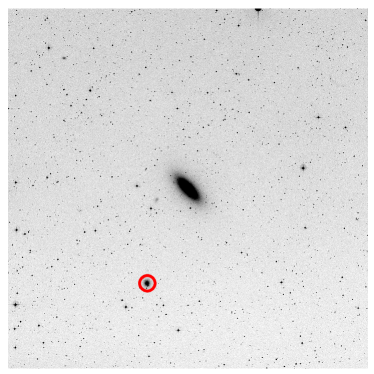
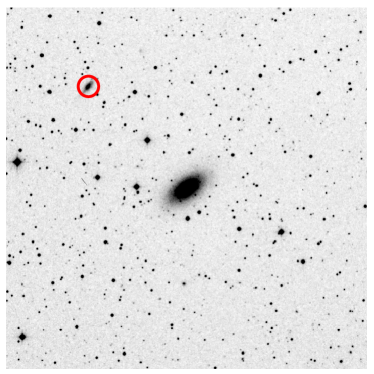
Figure 1: ESO Digital Sky Survey (DSS) images of NGC 3115 (left panel, $60^{\prime}\times 60^{\prime}$) and NGC 7457 (right panel $14.8^{\prime}\times 14.8^{\prime}$) and their companion galaxies, which are marked with red circles. North is up, and East to the left in both panels.

3 Data reduction and catalogues

The data from PN.S are rather unusual in form, and require a custom-built analysis package for their analysis. The details of the pipeline are presented in Douglas et al. (2002, 2007) and Merrett et al. (2006); here we give a brief summary of the main steps, describe some recent upgrades to its capabilities, and tabulate the resulting catalogues of PNe.

3.1 The Planetary Nebula Spectrograph and the reduction pipeline

The PN.S, described in detail in Douglas et al. (2002), is a slitless spectrograph that works using a counter-dispersed imagining technique (Fehrenbach, 1948, 1947a, 1947b). Two images of the same field are taken at the same time through a slitless spectrograph equipped with a narrow-band [OIII] filter to restrict the spectral range, and they are dispersed in opposite directions. Thus, stars in the field appear in the image as short segments of spectrum around 5007 Å  while the PNe appear as point sources due to their monochromatic emission. The exact position of a PN [O iii] 5007 Å line in each image depends on both its position on the sky and its observed wavelength, so matching up the detected PNe in pairs from the images dispersed in opposite directions makes it possible to obtain both their positions and velocities in a single step.

To extract this information, we have developed a specialised reduction pipeline for the instrument. The first step in the reduction is to create individual distortion-corrected images. This step includes the creation of a bad pixel mask, cosmic ray removal, and finally the undistortion of each image using arc lamp exposures obtained through a calibrated grid mask. As a second step, all images for a given galaxy are aligned and stacked, weighted according to the seeing, transparency etc. Although stars appear elongated into trails in the dispersed images, their centroids are still sufficiently well defined for them to be used to perform an astrometric calibration, based on the corresponding star coordinates in the USNO catalogue. At this point, the images are fully reduced, and we are ready to extract the PNe data from them.

The procedure for extracting a catalogue of PNe from these images is semi-automated, initially using Sextractor (Bertin & Arnouts, 1996) to find potential objects. As explained above, PNe in the images appear as point-like sources, since they emit only in the 5007 Å line within the wavelength range selected by the filter. With Sextractor, experimentation shows that these real sources can be distinguished from residual cosmic rays and other image defects by selecting only those objects that comprise a group of at least 5 contiguous pixels whose individual fluxes are at least 0.7 times the rms of the background.

There is, however, still the possibility of contamination from foreground stars and background galaxies. Fortunately, such sources are elongated along the dispersion direction due to their continuum light emission, with the length of elongation dictated by the filter bandpass. To identify such objects automatically, we create two further images. The first is an unsharp mask formed by smoothing the original spectral image with a $49\times 49$ median filter, and subtracting the smoothed image from the original. The second is obtained by convolving this median-subtracted image with an elliptical Gaussian function elongated in the dispersion direction. The resulting images are almost the same for extended stellar trails, but the point-like PNe are fainter in the smoothed version. Thus, for either arm, we can extract a catalogue that excludes any continuum sources by matching up source detections, and selecting only sources whose difference in magnitude between the median-subtracted image and its smoothed counterpart is larger than 0.5 mag (again tuned by experimentation).

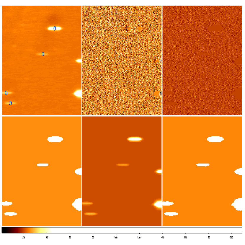
Figure 2: Different steps of the star trail removal routine, the top right panel show the resulting image. Refer to text for major details.

Although this automated process, which we have used in our previous pipeline processing, detects the vast majority of PNe, there are still a number of missed detections when the object is projected near a star trail. We have therefore developed a further technique to subtract out the star trails as an aid to detecting PNe, illustrated in Figure 2. We create a $25\times 1$ median-filtered image (top left panel) and subtract it from the science image, obtaining the median-subtracted image shown in the top middle panel. This image smooths away most of the star trails and leaves PNe almost unaffected. However, there are still residual features from the brighter parts of the brightest star trails that could be misidentified as PNe. We must therefore create a mask to exclude these regions. To do so, we further apply a $81\times 81$ median filter to the $25\times 1$ median filtered image to obtain an image that picks out the stars while removing the PNe. To turn this image into a mask, we run Sextractor on it and perform a morphological dilation on the segmentation map shown in the bottom left panel, by blurring (bottom middle panel) and thresholding (bottom right panel) the image. Applying this mask, by replacing masked values with zero, then yields the final trail-free data frame shown in the top right panel, which can then be pipeline processed in the way described above, with no residual confusion due to foreground stars.

With this modification, the only PNe missed by the automated process are those that lie very near the edge of the image, where the effectiveness of median filtering is limited, or near the centre of the target galaxy, where the bright continuum is noisy and difficult to subtract fully. However, the numbers are now sufficiently small that any remaining PNe are easily added in manually.

Finally the catalogues obtained in this way for the two arms of the spectrograph are matched up. Any pairs that appear at the same location in the undispersed direction to within two pixels, so have consistent spatial coordinate, and lie within a few hundred pixels of each other in the dispersed direction, so are consistent with the likely offset due to their Doppler shifts in the counter-dispersed frames, are identified as images of a single PN. Any object that does not appear in both arms is rejected as spurious. As a final check, each putative detection is assessed manually by three independent team members, by checking its location in the original stacked images, and an object is accepted in the catalogue if at least two classifiers confirm that it is real.

The wavelength and astrometric solutions derived above then allow us to obtain the mapping

$$\{x_{l},y_{l},x_{r},y_{r}\}\rightarrowtail\{x_{0},y_{0},\lambda\},$$ (1)

where $x_{l},y_{l},x_{r},y_{r}$ are the coordinates of the PNe in the left and right-dispersed images, $x_{0}$ and $y_{0}$ are the true sky coordinates and $\lambda$ is the wavelength of emission for each object. The emission wavelength translates directly into a line-of-sight velocity via the Doppler formula.

Errors are assigned to these velocities by propagating the errors in the assigned values of $x_{l},y_{l},x_{r},y_{r}$ through the transformation, further allowing for the uncertainty in the dispersion solution itself. A check on these uncertainties is provided by the fact that the observation of NGC 3384 presented here overlaps with the field containing NGC 3379 published by Douglas et al. (2007). Matching the catalogues results in 25 objects in both observations for which the RMS difference between the data is $20\,{\rm km}\,{\rm s}^{-1}$, implying an average error in each individual observation of $14\,{\rm km}\,{\rm s}^{-1}$, consistent with what the internal error analysis assigned.

3.2 The catalogues

The resulting catalogues of PNe are presented in Tables 3–7. The data for NGC 1023 are not shown here, since they were published in Noordermeer et al. (2008). For completeness, Table 7 also contains the 9 PNe identified as belonging to NGC 3384 in the adjacent observation of NGC 3379 by Douglas et al. (2007).

Table 3: Catalogue of PNe in NGC 3115.

ID	RA	Dec	Vhelio	m
	J2000	J2000	[km/s]	[mag]
PNS-EPN-N3489-01	10:04:51	-07:44:57	645.58	-
PNS-EPN-N3489-02	10:04:54.9	-07:43:55.5	845.18	18.96
PNS-EPN-N3489-03	10:04:55.5	-07:43:37.4	307.08	19.1
PNS-EPN-N3489-04	10:04:57.1	-07:46:22.8	568.28	18.65
.	.	.	.	.
.	.	.	.	.
.	.	.	.	.
PNS-EPN-N3489-188	10:05:36.2	-07:41:28.1	804.58	17.56
PNS-EPN-N3489-189	10:05:36.5	-07:41:49.7	722.08	19.17

Notes: Details on the velocity and positional errors are given in Section3.1. Velocities, measured from the [O iii] 5007 Å line, are corrected to heliocentric. The full catalogue is available at the CDS.

Table 4: Catalogue of PNe in NGC 7457.

ID	RA	Dec	Vhelio	m
	J2000	J2000	[km/s]	[mag]
PNS-EPN-N7457-001	23:00:42.75	30:10:10.7	993.94	20.4
PNS-EPN-N7457-002	23:00:48.31	30:08:58.2	870.64	20.24
PNS-EPN-N7457-003	23:00:51.14	30:09:19	886.94	19.5
PNS-EPN-N7457-004	23:00:51.42	30:09:44.1	939.94	19.69
.	.	.	.	.
.	.	.	.	.
.	.	.	.	.
PNS-EPN-N7457-112	23:01:8.34	30:08:24.6	755.84	19.98
PNS-EPN-N7457-113	23:01:10.11	30:06:58.2	724.74	19.83

Notes: Details on the velocity and positional errors are given in Section3.1. Velocities, measured from the [O iii] 5007 Å line, are corrected to heliocentric. The full catalogue is available at the CDS.

Table 5: Catalogue of PNe in NGC 2768.

ID	RA	Dec	Vhelio	m
	J2000	J2000	[km/s]	[mag]
PNS-EPN-N2768-01	09:10:56.13	60:03:21.9	1181.3	20.86
PNS-EPN-N2768-02	09:10:59.59	60:02:13.7	1133.9	21.86
PNS-EPN-N2768-03	09:10:59.86	60:03:38.5	1134.4	21.05
PNS-EPN-N2768-04	09:11:1.34	60:03:3.1	1172.1	20.49
.	.	.	.	.
.	.	.	.	.
.	.	.	.	.
PNS-EPN-N2768-314	09:12:15.08	60:03:8.9	1556.4	20.36
PNS-EPN-N2768-315	09:12:15.22	60:00:3.6	1595.6	21.08

Notes: Details on the velocity and positional errors are given in Section3.1. Velocities, measured from the [O iii] 5007 Å line, are corrected to heliocentric. The full catalogue is available at the CDS.

As well as the positions and line-of-sight velocities of the PNe, these tables also show the instrumental magnitude of each object, as derived from the images; since we only use these magnitudes to assess the strength of the detection and to investigate the shape of the planetary nebula luminosity function (see Section 4), no photometric calibration is required.

Table 6: Catalogue of PNe in NGC 3489.

ID	RA	Dec	Vhelio	m
	J2000	J2000	[km/s]	[mag]
PNS-EPN-N3489-01	11:00:09.1	13:53:21.3	660.52	16.49
PNS-EPN-N3489-02	11:00:09.2	13:55:26.3	663.62	16.59
PNS-EPN-N3489-03	11:00:09.6	13:51:25.7	1012.62	19.17
PNS-EPN-N3489-04	11:00:10.4	13:53:45.1	1418.92	16.49
.	.	.	.	.
.	.	.	.	.
.	.	.	.	.
PNS-EPN-N3489-59	11:00:23.7	13:54:43.8	742.12	15.82
PNS-EPN-N3489-60	11:00:27.4	13:54:41.6	591.12	16.62

Notes: Details on the velocity and positional errors are given in Section3.1. Velocities, measured from the [O iii] 5007 Å line, are corrected to heliocentric. The full catalogue is available at the CDS.

Table 7: Catalogue of PNe in NGC 3384.

ID	RA	Dec	Vhelio	m
	J2000	J2000	[km/s]	[mag]
PNS-EPN-N3384-01	10:47:54.8	12:36:48.5	822.6	18.75
PNS-EPN-N3384-02	10:47:54.9	12:36:15.8	1038.7	19.01
PNS-EPN-N3384-03	10:47:55.1	12:36:16.8	868.1	18.98
PNS-EPN-N3384-04	10:47:57.1	12:36:02.8	908.7	18.86
.	.	.	.	.
.	.	.	.	.
.	.	.	.	.
PNS-EPN-N3384-94	10:48:31.2	12:39:02.6	646.9	18.41
PNS-EPN-N3384-95	10:48:33.2	12:36:26.9	629	18.23

Notes: Details on the velocity and positional errors are given in Section3.1. Velocities, measured from the [O iii] 5007 Å line, are corrected to heliocentric. The full catalogue is available at the CDS.

4 The PNe Spatial Distribution and its Normalisation

As discussed in the Introduction, one concern with using PNe as tracers is that they may not be representative of the whole stellar population, but rather a subcomponent, which may introduce a bias in the dynamical analysis. This issue has already been thoroughly addressed in the context of ellipticals (Coccato et al., 2009; Napolitano et al., 2009, 2011), but now we need to establish the same point for S0s. Indeed, similar findings for S0s and ellipticals would not only confirm the effectiveness of the technique, but might also allow us to draw connections between the two types of galaxy.

4.1 Spatial distribution

The simplest test we can make is to compare the spatial distribution of PNe to that of the underlying stellar population: if PNe are effectively a random sampling of stars, then, to within a normalisation factor, the two should be the same.

We have therefore fitted elliptical isophotes to images of the galaxies in the sample, and plotted the surface brightness profiles extracted from these fits in Figure 3. In most instances, the images used were the $K$-band observations from the 2MASS survey (Skrutskie et al., 2006). In the case of NGC 3489, the galaxy is too faint to be reliably fitted using this data, but fortunately this galaxy lies in the region surveyed by SDSS (York et al., 2000), so we used their $z$-band image as a substitute: since we are only interested in matching the shape of the brightness profile, this red band traces the old stellar population as well as the $K$-band, and no colour correction is required. Finally, in the case of NGC 1023 we made use of a deep $R$-band image that we had previously analysed to determine the size of the region compromised by light from NGC 1023A, to exclude it from the analysis (Cortesi et al., 2011).

Typically, the PNe extend to larger radii than the reliable photometric fits shown in Figure 3. In order to extrapolate the comparison to these large radii, we have also fitted the images with a simple two-component disk+bulge model using GALFIT (Peng et al., 2002), and obtained the total surface brightness profile, resulting in the lines shown in Figure 3.

In order to compare these profiles to the PNe data, we need to correct the latter for incompleteness. Since PNe are primarily lost against the bright central parts of the galaxy, failing to correct for this effect would grossly distort their spatial profile. We carry out this correction in two stages, following a process developed by Coccato et al. (2009). First, we randomly place simulated PNe of varying magnitudes in model images that reproduce the noise properties of the real data, to establish the brightness level to which PNe can in general be reliably detected. We quantify this limits by $m_{80}$, the magnitude limit at which 80% of the simulated PNe are recovered. An illustration of this process is shown in Figure 4. Next, we populate the real science data with simulated PNe drawn from the known planetary nebula luminosity function (PNLF), brighter than an $m_{80}$ completeness limit, and see what fraction are lost against the bright galaxy continuum, star trails, etc, as a function of position, as illustrated in Figure 5. Finally, we correct for this incompleteness in the number counts of PNe as a function of radius, plotted in Figure 3.

In the central parts of these galaxies, incompleteness is too great to be corrected reliably, but, as Figure 3 shows, in the region of overlap with the photometric data, out into the extrapolation of the model fit, the agreement between the profiles of PNe and the stellar continuum is very good, typically over at least a factor of ten in brightness. There is therefore no evidence that the PNe are anything other than a fair sample of the stellar population.

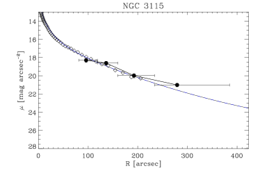
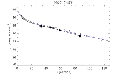
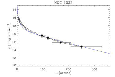
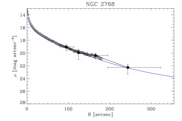
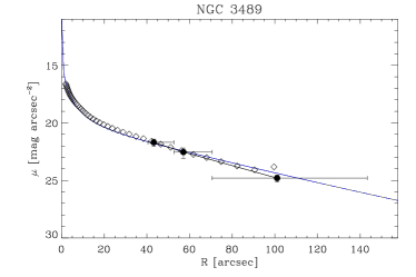
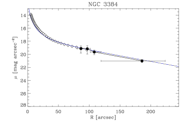
Figure 3: Surface density profiles of PNe and stars. Open diamonds: surface brightness profiles obtained with ellipse fitting of the galaxy image. Filled circles: PNe number density, computed as $-2.5LogNc/A$, where $Nc$ is the completeness corrected number of PNe with $m<m_{80}$ in the radial bin, and $A$ is the area of the circular anulus. Blue lines represent the extrapolation of the sersic + exponential disk fit to the stellar surface brighness data.

Figure 4: Recovered number of point like sources as a function of magnitude. The simulated PNe are added on an artificial image that mimic the sky and CCD noise, the recovered number decreases for fainter objects, see text for further details.

Figure 5: Number of detected point like sources with $m>m_{80}$ as a function of radius; the simulated objects are added to the science image. The incompleteness at small radii is caused by the bright continuum of the galaxy, see text for further details.

Figure 6: The observed PNLF and the fitted analytic function (Ciardullo et al., 1989) of NGC 3115, see text for further details.

4.2 The specific frequency of PNe

Having established that the proportionality between PNe numbers and stellar luminosity seems to be valid, we can now calculate the proportionality constant. This factor, usually designated $\alpha$ (Jacoby, 1980), is of interest because it relates to the stellar evolution of the particular population. So, for example, assessing how similar it is between ellipticals and S0s provides an independent route for determining how closely related these objects are, in this case in terms of the evolution of their stellar populations. Such a similarity would also add further justification for the view that PNe in S0s have a similar relation to the underlying stellar population as those in ellipticals, and hence that they can be used as similar kinematic tracers.

In fact, there is already evidence that this proportionality varies in interesting ways with the global properties of the galaxy. Although $\alpha$ is close to universal in value, it does vary systematically with colour (Hui et al., 1993), with the reddest ellipticals being poorer in PNe per unit galaxy luminosity than spirals (Buzzoni et al., 2006). This is somewhat counter-intuitive, as one might expect a star-forming spiral to have more of its luminosity provided by massive young stars that will never form PNe (Buzzoni et al., 2006). However, there are other ways in which the $\alpha$ parameter might be reduced. For example, if PNe have systematically shorter lifetimes in elliptical galaxies, one would expect to see fewer of them in any snapshot view. Alternatively, some stars with particular chemical properties might avoid becoming PNe at all, perhaps by losing their envelopes at an earlier stage. Support for this suggestion comes from the rather tight anti-correlation observed between $\alpha$ and the amount of far ultra-violet (FUV) emission from the galaxy: in an old stellar population, FUV emission could well arise from AGB stars that have already lost their envelopes, thus avoiding later evolution into PNe (Buzzoni et al., 2006).

We therefore now calculate the $\alpha$ parameter for the sample S0 galaxies, to see how they compare to those already determined for ellipticals (Coccato et al., 2009). The value of $\alpha$ obviously depends on how far down the PNLF one counts PNe away from the brightest magnitude observed. This brightest magnitude is well-defined by a sharp cut-off in the PNLF at a magnitude $m^{*}$, which we can measure by fitting the Ciardullo et al. (1989) analytic approximation to the data, as illustrated in Figure 6 (kept in instrumental magnitudes since an absolute value is not required). The value of $\alpha$ then depends on how far below $m^{*}$ one counts PNe. For a direct comparison with the ellipticals, we follow the same definition as Coccato et al. (2009), which involves counting the number of PNe with apparent magnitudes down to $m^{*}+1$. We then calculate $\alpha_{B,1.0}$, which is the ratio of this number of PNe to the total $B$-band luminosity over the range of radii that PNe have been observed. The radial range used for each galaxy in this survey is listed in Table 8.

In practice, our data generally probe to magnitudes significantly fainter than $m^{*}+1$: Table 8 lists the values of $m^{*}-m_{80}$ which quantifies how many magnitudes below $m^{*}$ the data remain reasonably complete. In order to use all this information in determining $\alpha$, we calculate the constant of proportionality counting PNe all the way down to this limiting magnitude, $\alpha_{B,m^{*}-m_{80}}$, and then use the known shape of the PNLF to correct its value to the adopted common metric quantity,

$$\alpha_{B,1.0}=\alpha_{B,m^{*}-m_{80}}\frac{\int_{m^{*}}^{m^{*+1}}F(m^{*},m^{{}^{\prime}})dm^{{}^{\prime}}}{\int_{m^{*}}^{m_{80}}F(m^{*},m^{{}^{\prime}})dm^{{}^{\prime}}},$$ (2)

where $F(m^{*},m)$ is the universal analytic approximation to the PNLF found by Ciardullo et al. (1989). The values for $\alpha_{B,1.0}$ determined in this way are listed in Table 8.

Table 8: $\alpha_{B,1.0}$ parameter and UV excess for the galaxy sample.

Name	Npn	Npn,corr	Rmin	Rmax	$m_{*}-m_{80}$	$\alpha_{B,1.0}$	(FUV-V)	Bt
			[arcs]	[arcs]	[mag]	$10^{9}\cdot L_{\odot}$	[mag]	[mag]
NGC 3115	$182$	$186$	$45.9$	$389.8$	$-3.0$	$1.0\pm 0.2$	$7.6\pm 0.1$	$-20.03\pm 0.13$
NGC 7457	$94$	$156$	$10.6$	$115.4$	$-1.9$	$8.4\pm 3.0$	$8.1\pm 0.1$	$-18.69\pm 0.32$
NGC 2768	$201$	$289$	$25.1$	$328.0$	$-1.6$	$2.1\pm 0.6$	$7.6\pm 0.1$	$-20.89\pm 0.34$
NGC 1023	$133$	$236$	$21.7$	$332.4$	$-2.5$	$2.5\pm 0.6$	$7.6\pm 0.1$	$-19.10\pm 0.28$
NGC 3489	$50$	$75$	$20.3$	$146.0$	$-3.3$	$1.9\pm 0.8$	$6.6\pm 0.1$	$-20.05\pm 0.22$
NGC 3384	$75$	$77$	$43.6$	$228.1$	$-2.6$	$2.3\pm 0.9$	$7.5\pm 0.1$	$-19.41\pm 0.19$

Notes: Col. 1: Galaxy name. Col. 2: Number of PNe with $m<m_{80}$. Col. 3: Number of PNe with $m<m_{80}$ once corrected for completeness. Col. 4: Galactocentric radius of the innermost detected PN. Col. 5: Galactocentric radius of the outermost detected PN. Col. 6: Difference between the PNLF bright cut-off ($m_{*}$) and $m_{80}$ (see Section 4.2). Col. 7: $\alpha$ parameter in the $B$-band, integrating the PNLF from $m_{*}$ to $m_{*}+1$ mag (see Section 4.2). Col. 8: UV excess, from the Galaxy Evolution Explorer (GALEX). Col. 9: $B$-band absolute magnitude, from the apparent magnitudes in the RC3 catalogue and the distance moduli of Tonry et al. (2001), shifted by $-0.16$ magnitudes, see text for details.

Having calculated these $\alpha$ values, we can now compare them to the values determined in the same way for ellipticals by Coccato et al. (2009). Figure 7 shows the resulting comparisons when combining $\alpha$ values with optical colours, FUV excess and absolute magnitude. Plotted against optical colour, the S0s $\alpha$ values are indistinguishable from ellipticals, and seem to show the same trend described above that bluer galaxies have higher specific frequencies of PNe. Similarly, when we investigate their FUV fluxes, obtained from the Galaxy Evolution Explorer (GALEX) and corrected for extinction using the relation $A_{FUV}=8.376E(B-V)$ (Wyder et al., 2005), we find that the S0s lie in the same part of the plot as ellipticals, although the range of FUV excesses for the S0s is too small to really see if they follow the same strong trend. Finally, we compare $\alpha$ to the $B$-band absolute magnitudes, which were obtained from the apparent magnitudes in the RC3 catalogue and the distance moduli of Tonry et al. (2001), shifted by $-0.16$ magnitudes to take into account the newer Cepheid zero-point of Freedman et al. (2001), for consistency with Coccato et al. (2009). There is an interesting suggestion of a correlation between $\alpha$ and $FUV-V$ for S0s in Figure 7, which is strengthened by the fact that two of the elliptical galaxies that lie closest to the S0s (NGC 4564 and NGC 3377) were found by Coccato et al. (2009) to have disk like kinematics, and thus may well be S0s themselves. However, the numbers are still sufficiently small that the only firm conclusion is that S0s lie in the same region of these plots as ellipticals, and hence that the stellar evolutionary properties that they probe are indistinguishable, adding further confidence to the use of PNe as a common stellar kinematic probe in these galaxy types.

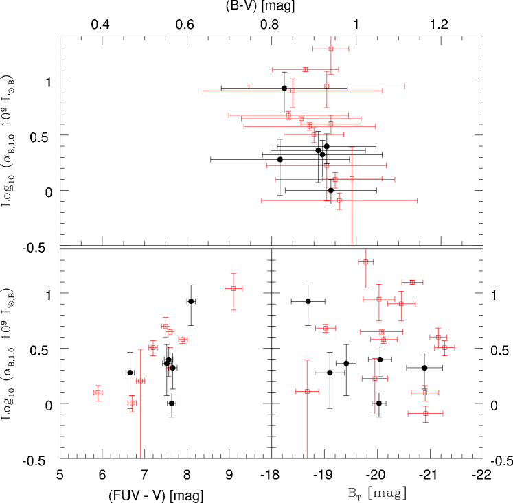
Figure 7: Relationships for elliptical and S0 galaxies between $\alpha_{B,1.0}$ parameter and UV excess (bottom left panel), absolute $B$-band magnitude (bottom-right panel) and (B-V) colour (upper panel). Red open squares show the values of the elliptical sample presented in Coccato et al. (2009), while filled black circles correspond to S0s from the present study.

5 Velocity maps and kinematics

In this section we present the resulting stellar kinematics. Figure 8 shows the PNe data superimposed on the Digitised Sky Survey (DSS) image of each galaxy in the sample. The incompleteness at small radii due to the bright galaxy continuum, discussed in Section 4, is very apparent. However, these plots also show the large radii to which PNe can be detected in these data, which underlines how nicely they complement conventional kinematic data: the point where the continuum becomes too faint to obtain good absorption-line data is just where PNe become readily detectable, and they remain present in significant numbers out to the very faint surface brightnesses illustrated in Figure 3.

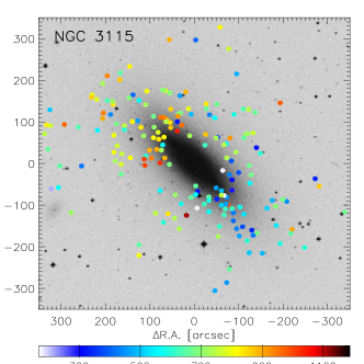
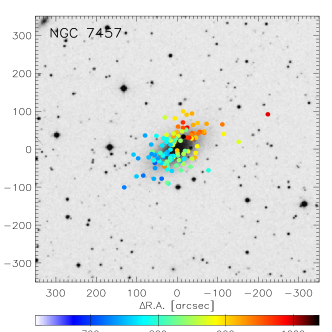
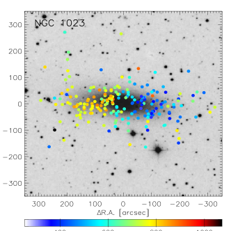
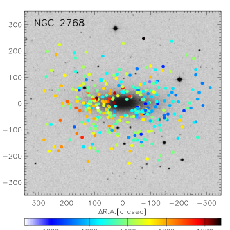
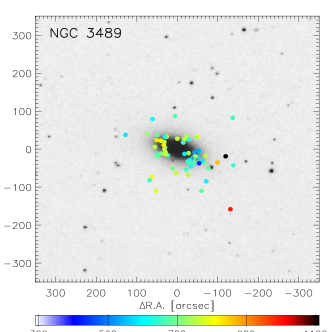
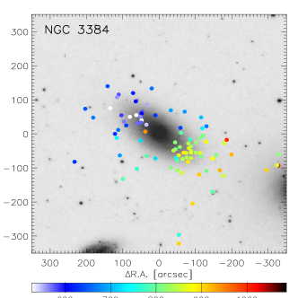
Figure 8: DSS images of the sample galaxies, with the PNe positions marked with circles. The color of the circles represent the measured radial velocity of the PNe, according to the velocity scales below each panel. First row: field S0s, second row: S0s in groups, third row: S0s in rich groups.

It is apparent from Figure 8 that most of these galaxies are characterised by obvious rotation, although there is also a significant amount of random motion. It also appears that the balance between ordered and random motion differs from galaxy to galaxy; for example NGC 7457 seems to show more coherent motions than NGC 3115. To quantify such differences in a preliminary kinematic analysis, we derive the rotation velocity and random motions assuming that each galaxy can be described as a single-component thin disk. Following Cortesi et al. (2011), a maximum likelihood analysis is employed to determine in a series of radial bins the mean streaming velocity and the two components of random motion in the tangential and radial directions, here assumed to be coupled together by the epicycle approximation. To minimise distortion of the fit by outlier PNe, the analysis iteratively rejects objects whose deviation from the mean velocity in each bin is higher than 2.1 $\sigma$; in no case are more than $7\%$ of the total number of PNe rejected by this process, offering some reassurance that such a disk model is not unreasonable.

As Figure 9 illustrates, this analysis confirms the impression that the balance between ordered and random motion varies significantly between galaxies. It also offers one final very useful check on the reliability of PNe as stellar kinematic tracers, as we can compare the results to those from conventional absorption-line spectra. Figure 9 therefore also shows such absorption-line kinematics for the major axes of these galaxies, as obtained from various published sources (Debattista et al., 2002; Caon et al., 2000; Simien & Prugniel, 1997; Norris et al., 2006; Fisher, 1997). Although the comparison is not exact, these systems are sufficiently close to edge on that the conventional major-axis velocity dispersion data should lie close to $\sigma_{\phi}$ in the PNe data if both are measuring the same kinematic population. These plots underline the complementarity between conventional absorption-line data and PNe kinematics, as the latter take over just where the former run out. It is also clear that there is no inconsistency between these data sets, demonstrating once again that they are probing the same kinematic population.

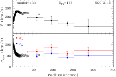
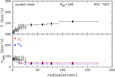
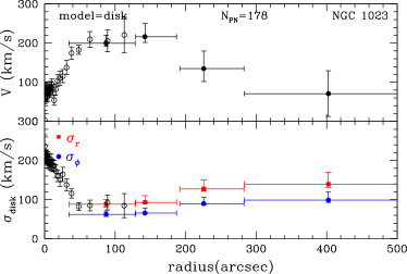
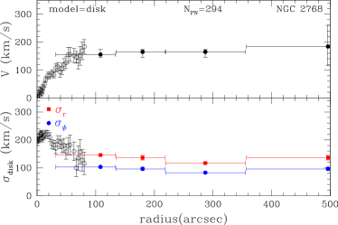
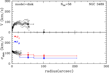
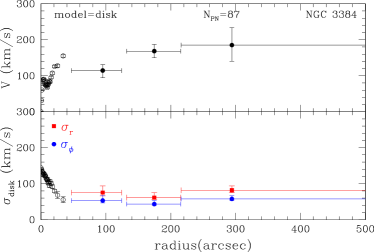
Figure 9: Kinematics of the S0 sample derived using the disk model of Cortesi et al. (2011). First row: field galaxies, second row: group members, third row: rich group members. The black circles show the average velocity in the bin (whose size is represented by the horizontal error bars). The red squares and blue circles show the velocity dispersion along the radial and azimuthal directions respectively. The stellar velocities and velocity dispersions obtained from absorption line spectra (Caon et al., 2000; Simien & Prugniel, 1997; Norris et al., 2006; Fisher, 1997) are shown as empty black circles. The number of PNe left after the clipping performed in each likelihood fit is annotated at the top of the corresponding panel.

6 Conclusions

This paper has presented the data for the first systematic survey of S0 kinematics as a function of environment, using PNe to trace their stellar velocities out to large radii. In the process, we have presented a series of tests on the viability of using PNe for such a study, demonstrating that they really are representative of the underlying stellar population. The PNe pass all these tests: they show the same spatial distribution as the starlight; their numbers are consistent with those found in comparable elliptical galaxies where their use as kinematic tracers is well established; and their kinematics join smoothly onto those derived from conventional stellar data at smaller radii.

As well as demonstrating that PNe are good tracers of the stellar populations, and therefore that the catalogues presented in this paper are a unique dataset to study the kinematics and dynamics of lenticular galaxies, we have also shed some light on the nature of S0 galaxies. In particular, the similarity of their $\alpha$ parameters to those found in elliptical galaxies implies that, at least at the stellar population level, these two classes of object are very similar. Unsurprisingly their kinematics are rather different, being in most cases dominated by rotational motion. There is however significant variety in these kinematics, with rotation velocities that vary in differing ways with radius and differing balances between ordered and random motion. The initial inspection of these properties in Figure 9 does not reveal any obvious trends with the richness of environment, suggesting that this may not be a dominant factor in the choice of channel by which S0s form. However, Cortesi et al. (2011) already established that these simple kinematic properties can be rather misleading due to cross-contamination between disk and bulge kinematics, and that a clear picture only emerges when the kinematic components are carefully separated. Indeed, by breaking S0 galaxies down into these components, we hope to find subtler indications as to where these systems lie in the overall story of galaxy morphology by, for example, comparing their spheroidal components to ellipticals and to the bulges of spirals. We will present such an analysis in a subsequent paper, to seek the definitive answers from the survey data presented here.

References

- Aragón-Salamanca (2008) Aragón-Salamanca, A. 2008, in IAU Symposium, Vol. 245, IAU Symposium, ed. M. Bureau, E. Athanassoula, & B. Barbuy, 285–288
- Bertin & Arnouts (1996) Bertin, E. & Arnouts, S. 1996, A&AS, 117, 393
- Bournaud et al. (2005) Bournaud, F., Jog, C. J., & Combes, F. 2005, A&A, 437, 69
- Buzzoni et al. (2006) Buzzoni, A., Arnaboldi, M., & Corradi, R. L. M. 2006, MNRAS, 368, 877
- Byrd & Valtonen (1990) Byrd, G. & Valtonen, M. 1990, ApJ, 350, 89
- Caon et al. (2000) Caon, N., Macchetto, D., & Pastoriza, M. 2000, ApJS, 127, 39
- Capaccioli et al. (1986) Capaccioli, M., Lorenz, H., & Afanasjev, V. L. 1986, A&A, 169, 54
- Ciardullo et al. (1989) Ciardullo, R., Jacoby, G. H., Ford, H. C., & Neill, J. D. 1989, ApJ, 339, 53
- Coccato et al. (2009) Coccato, L., Gerhard, O., Arnaboldi, M., et al. 2009, MNRAS, 394, 1249
- Cortesi et al. (2011) Cortesi, A., Merrifield, M. R., Arnaboldi, M., et al. 2011, MNRAS, 414, 642
- de Vaucouleurs et al. (1976) de Vaucouleurs, G., de Vaucouleurs, A., & Corwin, H. G. 1976, 2nd reference catalogue of bright galaxies containing information on 4364 galaxies with reference to papers published between 1964 and 1975
- de Vaucouleurs et al. (1991) de Vaucouleurs, G., de Vaucouleurs, A., Corwin, Jr., H. G., et al. 1991, Third Reference Catalogue of Bright Galaxies. Volume I: Explanations and references. Volume II: Data for galaxies between 0h and 12h. Volume III: Data for galaxies between 12h and 24h.
- Debattista et al. (2002) Debattista, V. P., Corsini, E. M., & Aguerri, J. A. L. 2002, MNRAS, 332, 65
- Dekel et al. (2005) Dekel, A., Stoehr, F., Mamon, G. A., et al. 2005, Nature, 437, 707
- Douglas et al. (2002) Douglas, N. G., Arnaboldi, M., Freeman, K. C., et al. 2002, PASP, 114, 1234
- Douglas et al. (2007) Douglas, N. G., Napolitano, N. R., Romanowsky, A. J., et al. 2007, ApJ, 664, 257
- Doyle et al. (2005) Doyle, M. T., Drinkwater, M. J., Rohde, D. J., et al. 2005, MNRAS, 361, 34
- Dressler (1980) Dressler, A. 1980, ApJ, 236, 351
- Fehrenbach (1947a) Fehrenbach, C. 1947a, Annales d’Astrophysique, 10, 257
- Fehrenbach (1947b) Fehrenbach, C. 1947b, Annales d’Astrophysique, 10, 306
- Fehrenbach (1948) Fehrenbach, C. 1948, Annales d’Astrophysique, 11, 35
- Fisher (1997) Fisher, D. 1997, AJ, 113, 950
- Forbes et al. (2012) Forbes, D. A., Cortesi, A., Pota, V., et al. 2012, ArXiv e-prints
- Fouque et al. (1992) Fouque, P., Gourgoulhon, E., Chamaraux, P., & Paturel, G. 1992, A&AS, 93, 211
- Freedman et al. (2001) Freedman, W. L., Madore, B. F., Gibson, B. K., et al. 2001, ApJ, 553, 47
- Gunn & Gott (1972) Gunn, J. E. & Gott, III, J. R. 1972, ApJ, 176, 1
- Hubble (1936) Hubble, E. P. 1936, Realm of the Nebulae (Yale University Press)
- Hui et al. (1993) Hui, X., Ford, H. C., Ciardullo, R., & Jacoby, G. H. 1993, ApJ, 414, 463
- Jacoby (1980) Jacoby, G. H. 1980, ApJS, 42, 1
- Kronberger et al. (2008) Kronberger, T., Kapferer, W., Ferrari, C., Unterguggenberger, S., & Schindler, S. 2008, A&A, 481, 337
- Merrett et al. (2006) Merrett, H. R., Merrifield, M. R., Douglas, N. G., et al. 2006, MNRAS, 369, 120
- Napolitano et al. (2011) Napolitano, N. R., Romanowsky, A. J., Capaccioli, M., et al. 2011, MNRAS, 411, 2035
- Napolitano et al. (2009) Napolitano, N. R., Romanowsky, A. J., Coccato, L., et al. 2009, MNRAS, 393, 329
- Noordermeer et al. (2008) Noordermeer, E., Merrifield, M. R., Coccato, L., et al. 2008, MNRAS, 384, 943
- Norris et al. (2006) Norris, M. A., Sharples, R. M., & Kuntschner, H. 2006, MNRAS, 367, 815
- Peng et al. (2002) Peng, C. Y., Ho, L. C., Impey, C. D., & Rix, H.-W. 2002, AJ, 124, 266
- Quilis et al. (2000) Quilis, V., Moore, B., & Bower, R. 2000, Science, 288, 1617
- Romanowsky et al. (2003) Romanowsky, A. J., Douglas, N. G., Arnaboldi, M., et al. 2003, Science, 301, 1696
- Simien & Prugniel (1997) Simien, F. & Prugniel, P. 1997, A&AS, 126, 519
- Skrutskie et al. (2006) Skrutskie, M. F., Cutri, R. M., Stiening, R., et al. 2006, AJ, 131, 1163
- Tonry et al. (2001) Tonry, J. L., Dressler, A., Blakeslee, J. P., et al. 2001, ApJ, 546, 681
- Williams et al. (2010) Williams, M. J., Bureau, M., & Cappellari, M. 2010, MNRAS, 409, 1330
- Wyder et al. (2005) Wyder, T. K., Treyer, M. A., Milliard, B., et al. 2005, ApJ, 619, L15
- York et al. (2000) York, D. G., Adelman, J., Anderson, Jr., J. E., et al. 2000, AJ, 120, 1579