Abstract

Using the Closed-Time-Path approach, we perform a systematic leading order calculation of the relaxation rate of flavour correlations of left-handed Standard Model leptons. This quantity is of pivotal relevance for flavoured Leptogenesis in the Early Universe, and we find it to be $5.19\times 10^{-3}T$ at $T=10^{7}\,{\rm GeV}$ and $4.83\times 10^{-3}T$ at $T=10^{13}{\rm GeV}$. These values apply to the Standard Model with a Higgs-boson mass of $125\,{\rm GeV}$. The dependence of the numerical coefficient on the temperature $T$ is due to the renormalisation group running. The leading linear and logarithmic dependencies of the flavour relaxation rate on the gauge and top-quark couplings are extracted, such that the results presented in this work can readily be applied to extensions of the Standard Model. We also derive the production rate of light (compared to the temperature) sterile right-handed neutrinos, a calculation that relies on the same methods. We confirm most details of earlier results, but find a substantially larger contribution from the $t$-channel exchange of fermions.

1 Introduction

The origin of the matter anti-matter asymmetry in the Universe is one of the most important open questions in Particle Physics and Cosmology. Leptogenesis [1] is among the most plausible possible mechanisms for generating the observed baryon asymmetry dynamically in the Early Universe. The recent discovery of a Standard Model (SM) like Higgs boson provides further support for this mechanism, where the asymmetry is generated by out-of-equilibrium decays of heavy sterile right-handed neutrinos into a Higgs boson and a lepton.

In recent years, substantial progress was made in the theoretical description of Leptogenesis using Non-Equilibrium Quantum Field Theory in the Closed Time Path (CTP) formalism [5, 6, 7]. Particular attention was given to the derivation of quantum evolution equations for distribution functions [8, 9, 10, 11, 12], the calculation of thermal corrections to the charge-parity ($CP$) asymmetry [13, 14, 15, 16, 17, 18, 19], and related questions [20, 21, 22, 23, 24, 25, 26, 27].

Interaction rates mediated by Higgs-Yukawa couplings are crucial for Leptogenesis predictions. The production and decay rates of the lightest right-handed neutrino determine the strength of the washout, and they are mediated by their Yukawa couplings $Y$ to SM lepton doublets and Higgs bosons, while the lepton flavour equilibration rate determines the temperature scale where flavour effects become relevant for calculations of the asymmetry [28, 29, 30], and it is mediated by the SM lepton Yukawa couplings $h$.

At low temperatures, both processes [right-handed neutrino (inverse) decays and flavour equilibration] are described at leading order (LO) through $1\leftrightarrow 2$ processes, namely decays and inverse decays, involving only the Higgs boson and left- and right-handed leptons and sterile neutrinos. At high temperatures, both rates are phase space suppressed. Therefore a complete LO calculation of these crucial interactions must include processes where additional gauge bosons are emitted or absorbed or where an intermediate Higgs boson decays into a pair of top quarks. For right-handed neutrino (inverse) decays, the LO analysis pertinent to high temperatures has first been performed in Refs. [31, 32]. In some earlier and also more recent papers [26, 33, 34, 35], the inclusion of the gauge interactions is restricted to the effect of the modified thermal dispersion relations (thermal masses), but these approaches should only partly capture the LO effects. Closely related to the problem of right-handed neutrino production and the relaxation of the flavour correlations of active leptons is the production of photons in a quark-gluon plasma, which is calculated e.g. in Refs. [36, 37].

Gauge boson corrections in the low temperature regime have recently received some attention in the works [38, 39], where a non-relativistic analysis including leading relativistic corrections has been performed. When the right-handed neutrino mass cannot be neglected, the tree-level scattering amplitudes exhibit infrared (IR) divergences, and the familiar cancellation of these with contributions from virtual diagrams has to be generalised to a finite-temperature environment. It turns out that the cancellation of IR divergences in the non-relativistic regime can be generalised to fully relativistic processes as well [40].

The main topic of this paper is the calculation of Higgs Yukawa mediated interaction rates in a high temperature background. We have performed this calculation using methods based on the two-particle-irreducible (2PI) CTP formulation of Non-Equilibrium Quantum Field Theory, within the framework that has been applied to calculate $CP$-violating rates in Refs. [11, 19]. A main advantage of the 2PI approach is that it directly gives rise to a derivation of the appropriate description of the physical screening that regulates the $t$-channel divergences that occur in certain tree-level scattering diagrams. The screening is implemented by the use of a resummed propagator, which in contrast appears as an ad hoc prescription within an approach based on the calculation of scattering matrix elements.

Presently, our main phenomenological interest is to perform a LO calculation of the damping rate of lepton flavour coherence, that is of importance for flavoured Leptogenesis. This flavour damping rate can be used as an input to the systematic analysis of flavour decoherence in Leptogenesis, that has been presented in Ref. [11]. Having obtained the various diagrammatic contributions to flavour damping, it is a simple matter to extract the (inverse) decay rates of right-handed neutrinos in the high temperature regime. We thereby confirm most details of the results presented in Refs. [31, 32], but find a substantially larger contribution from $t$-channel fermion exchange. The latter discrepancy should be due to a different technical implementation of the extraction of the coefficients of the logarithmically enhanced (in squares of the gauge coupling constant) and the standard perturbative contributions. In order to test our method, we have therefore compared its result to a fit to the numerically performed integral and found it to agree within the expected accuracy of the present approximations.

The remainder of this paper is organised as follows: In Section 2, we introduce the formalism and explain how the relevant interaction rates are obtained in this setup. Contributions to the interaction rates from self-energy type and vertex type diagrams are calculated in Sections 3 and 4 respectively, while collinearly enhanced $1\to 2$ processes are calculated in Section 5. The final numerical results and implications for phenomenology are presented in Section 6, before we conclude in Section 7.

2 Setup

2.1 Goal of the Calculation

The interactions that lead to the production of right-handed neutrinos $N_{i}$ are the Yukawa couplings $Y_{ia}$. The lepton asymmetry can be partly transferred from left-handed lepton doublets $\ell_{b}$ to right handed active leptons ${\rm R}_{a}$ through the Yukawa couplings $h_{ab}$. These also lead to the decoherence of off-diagonal correlations between the lepton flavours. Explicitly, these Yukawa interactions are given by the Lagrangian terms

$$-Y_{ia}\bar{\psi}_{Ni}\tilde{\phi}^{\dagger}P_{\rm L}\psi_{\ell a}-h_{ab}\phi^{\dagger}\bar{\psi}_{{\rm R}a}P_{\rm L}\psi_{\ell b}+{\rm c.c.}\,,$$ (1)

where ${\rm c.c.}$ stands for complex conjugation. Four-component spinors are denoted by $\psi$, and the subscripts indicate the fields that they are associated with. While a formulation in terms of Weyl spinors is also possible and perhaps more appropriate, we choose here four component spinors in order to make use of the standard identities for Dirac matrices for the simplification of the spinor algebra. The indices of ${\rm SU}(2)_{\rm L}$ are suppressed, the contraction of these between the fields $\phi$ and $\ell$ is implied, and $\tilde{\phi}=(\epsilon\phi)^{\dagger}$, where $\epsilon$ is the antisymmetric rank-two ${\rm SU}(2)_{\rm L}$ tensor.

The goal of this paper is to calculate interaction rates mediated by Yukawa couplings in a finite temperature, finite density environment like the Early Universe. Tree level $1\to 2$ processes that are proportional to $h^{2}$ are kinematically suppressed in the Early Universe, since all involved particles are massless (i.e. masses much smaller than the temperature) at temperatures $T$ above the Electroweak phase transition. Similarly, when $T\gg M_{N}$, where $M_{N}$ is the mass of the right-handed neutrino, the right-handed neutrinos can be approximated as massless, such that decays $N\to\phi\ell$ are suppressed.

With the tree-level $1\leftrightarrow 2$ channels forbidden or suppressed, the LO rates involve the radiation of one additional gauge boson, which leads to scattering rates that are parametrically of order $g^{2}h^{2}$ or $g^{2}Y^{2}$, respectively, where $g$ denotes a gauge coupling. At the same order, there are also contributions from collinearly enhanced $1\leftrightarrow 2$ processes when medium effects mediated by gauge interactions are resummed into the propagators [31]. Due to the sizable top-quark Yukawa coupling, a leading order calculation should also account for the Higgs boson decaying into a top-quark pair.

For the present calculation, we assume that all external particles are massless (before including thermal corrections), what leads to significant simplifications (i.e. the vanishing of numerous contributions from the CTP Feynman rules and the absence of soft and collinear IR divergences) that become apparent during the course of the calculation. Within the CTP formalism, the production and relaxation rates can be inferred from the collision term, as explained in Section 2.3. The collision terms for $N$, $\ell$ and ${\rm R}$ encompass similar diagrams, that are related among one another by an exchange of the Yukawa coupling matrices and the gauge coupling constants. In the following, we therefore derive the collision term for $\ell$, but we factorise the results in such a way that they can easily be employed in order to obtain the production and destruction rates for ${\rm R}$ and $N$ as well.

2.2 Definitions

We perform the calculation of the collision terms within the framework developed in Refs. [11, 19]. Here we just give the definitions that are relevant for the present calculation. The fermionic Wightman functions that appear in the collision term are

$${\rm i}S^{<}(k) =-2S^{\cal A}(k)f(k)\,,$$ (2a)

$${\rm i}S^{>}(k) =2S^{\cal A}(k)[1-f(k)]\,,$$ (2b)

where $S^{\cal A}(k)$ is the spectral function that determines the location of the quasi-particle poles and $f(k)$ is the distribution function that will be specified more precisely below. Tree-level propagators, which we indicate by a superscript $(0)$, are recovered when replacing the spectral function $S^{\cal A}$ with a delta distribution:

$$S^{(0){\cal A}}(k)=\pi P_{X}(\not{k}+m)\delta(k^{2}-m^{2}){\rm sign}(k^{0})\,.$$ (3)

In case of massless, chiral fermions, either $P_{X}=P_{{\rm L},{\rm R}}$ (i.e. $P_{\rm L}$ for $\ell$ and $P_{\rm R}$ for ${\rm R}$), whereas for Dirac and four-component Majorana fermions, $P_{X}=\mathbbm{1}$. The relations for the distribution functions are

$$f(k)=\left\{\begin{array}[]{l}f(\mathbf{k})\quad\textnormal{for}\quad k^{0}>0\\ 1-\bar{f}(\mathbf{k})\quad\textnormal{for}\quad k^{0}<0\end{array}\right.\qquad\textnormal{(fermions)}\,,$$ (6)

where $f(\mathbf{k})$ and $\bar{f}(\mathbf{k})$ are the distribution functions of particles and anti-particles. In kinetic equilibrium, the distributions are of the Fermi-Dirac form

$$f(k)=\frac{1}{{\rm e}^{\beta(k^{0}-\mu)}+1}\,,$$ (7)

where $\beta=1/T$. Note that $\mu$ and $f(k)$ may be hermitian matrices in order to take account of flavour coherence [11].

To calculate the self energies, we also need the bosonic Wightman functions for the Higgs and gauge bosons. For scalars, these are

$${\rm i}\Delta^{<}(k) =2\Delta^{\cal A}(k)f(k)\,,$$ (8a)

$${\rm i}\Delta^{>}(k) =2\Delta^{\cal A}(k)[1+f(k)]\,,$$ (8b)

where the tree-level spectral function for scalar particles of mass $m$ is given by

$$\Delta^{(0){\cal A}}(k)=\pi\delta(k^{2}-m^{2}){\rm sign}(k^{0})\,.$$ (9)

The distribution function $f(k)$ with the four-momentum as an argument can be related to the particle and anti-particle distributions $f(\mathbf{k})$ and $\bar{f}(\mathbf{k})$ as

$$f(k)=\left\{\begin{array}[]{l}f(\mathbf{k})\quad\textnormal{for}\quad k^{0}>0\\ -[1+\bar{f}(\mathbf{k})]\quad\textnormal{for}\quad k^{0}<0\end{array}\right.\qquad\textnormal{(bosons)}\,.$$ (12)

For distributions in kinetic equilibrium,

$$f(k)=\frac{1}{{\rm e}^{\beta(k^{0}-\mu)}-1}\,.$$ (13)

Finally we use gauge-boson propagators in Feynman gauge, such that

$${\rm i}\Delta^{<,>}_{\mu\nu}=-g_{\mu\nu}{\rm i}\Delta^{<,>}\,.$$

Evolution equations for the distribution functions $f(k)$ can be derived from the Dyson-Schwinger equations for the Wightman functions $S^{ab}$ and $\Delta^{ab}$. In Wigner space and to first order in gradients, the relevant equations for the the lepton doublet and for the right-handed neutrino are

$$i\partial_{t}\gamma^{0}S_{\ell}^{<,>}-\left[\mathbf{k}\cdot\mathbf{\gamma}\gamma^{0}+\Sigma\!\!\!/_{\ell}^{H}\gamma^{0},i\gamma^{0}S_{\ell}^{<,>}\right]-\left[i\Sigma\!\!\!/_{\ell}^{<,>}\gamma^{0},\gamma^{0}S_{\ell}^{H}\right]=-\frac{1}{2}\left(i{\cal C}_{\ell}+i{\cal C}_{\ell}^{\dagger}\right),$$ (14)

$$i\partial_{t}\gamma^{0}S_{N}^{<,>}=-i{\cal C}_{N}\,.$$ (15)

For a derivation of these equations and the further treatment of the left-hand sides we refer the reader to Refs. [11, 19]. Physical processes, like the Yukawa induced scattering and decay processes that we are interested in here, are encoded in the collision terms ${\cal C}$, as explained in more detail in the next Section.

2.3 Contributions to the Collision Term

In this Section and throughout most of the remainder of this paper, we consider the flavour relaxation rate for left-handed SM leptons $\ell$. The methods employed and the calculations performed readily give rise to the production rate of sterile right-handed neutrinos $N$, as it is explained in Section 2.5. Numerical results of this production rate together with a comparison to the earlier results of Refs. [31, 32] are presented in Section 6.2.

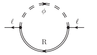
Figure 1: Diagram that represents the flavour-sensitive contribution to the lepton self energy ${\Sigma\!\!\!/}^{(1)}_{\ell}$, that occurs at one-loop order in the 2PI approach. Double lines indicate exact (in the present approach one-loop resummed) propagators and the external legs are understood to be amputated.

The collision term for the lepton doublets,

$${\cal C}_{\ell}(p) ={\rm i}{\Sigma\!\!\!/}_{\ell}^{>}(p){\rm i}S^{<}_{\ell}(p)-{\rm i}{\Sigma\!\!\!/}_{\ell}^{<}(p){\rm i}S^{>}_{\ell}(p)\,,$$ (16)

can be calculated perturbatively by employing a loop expansion of the leptonic self energy ${\rm i}{\Sigma\!\!\!/}_{\ell}^{<,>}$. Furthermore, the propagator ${\rm i}S_{\ell}^{<,>}$ contains self-energy insertions that may be of importance and that can also be expanded perturbatively. In this paper, we restrict ourselves to flavour-sensitive contributions that are at least of order $h^{2}$ in the Yukawa couplings and that we indicate by a superscript ${\rm fl}$, i.e. $\not{\Sigma}_{\ell}^{\rm fl}$ and ${\cal C}_{\ell}^{\rm fl}$. Due to the non-trivial flavour structure, these couplings will give rise to flavour decoherence, in contrast to the flavour-diagonal gauge couplings. The latter interactions are however of importance, as they open up the phase space for flavour-decohering processes (in combination with the coupling $h$) that would be kinematically forbidden otherwise. Moreover, gauge interactions maintain kinetic equilibrium for gauged particles, which is what we assume throughout this work.

Up to two loops, there are contributions to the flavour-sensitive rates from the one-loop self energy in Figure 1 and from the two-loop vertex-type diagrams in Figure 5, which are obtained from the self-energy diagram by connecting two different propagators with a gauge boson.

Note that in the 2PI approach, no two-particle-reducible diagrams appear where a gauge boson connects to both ends of the same propagator. Similarly, there is no diagrammatic contribution from the insertion of a top-loop into the Higgs boson propagator. While such diagrams with a self-energy insertion do not derive explicitly from the 2PI loop expansion of the effective action, self-energy insertions are of leading importance and are accounted for implicitly, by using resummed propagators to evaluate the collision terms. In fact, self-energy insertions in all propagators present in Figure 1 contribute to the flavour decoherence at LO. As we will see below, it is possible to expand the Higgs propagator up to the order of single loop insertions, whereas the lepton propagators must be maintained in the fully resummed form due to the presence of $t$-channel divergences from fermion exchange.

According to the loop expansion indicated in Figures 1 and 5, we decompose the collision term as

$${\cal C}^{\rm fl}_{\ell} ={\cal C}_{\ell}^{\rm self}+{\cal C}_{\ell}^{\rm vertex}.$$ (17)

The contribution from the lepton self-energy diagram, Figure 1, is given by

$${\rm i}\not{\Sigma}_{\ell}^{{\rm(1)}ab}(p)= h^{\dagger}\int\frac{d^{4}k}{(2\pi)^{4}}\frac{d^{4}q}{(2\pi)^{4}}(2\pi)^{4}\delta^{4}(p-k-q){\rm i}\Delta_{\phi}^{ab}(k){\rm i}S_{\rm R}^{ab}(q)h\,,$$ (18)

i.e.

$${\cal C}_{\ell}^{\rm self}={\rm i}{\Sigma\!\!\!/}_{\ell}^{(1)>}(p){\rm i}S^{<}_{\ell}(p)-{\rm i}{\Sigma\!\!\!/}_{\ell}^{(1)<}(p){\rm i}S^{>}_{\ell}(p)\,.$$ (19)

Within the 2PI approach, the propagators ${\rm i}S_{\ell,{\rm R}}$ and ${\rm i}\Delta_{\phi}$ are understood as the exact propagators. In the present work, we approximate these by propagators that contain the resummed one-loop corrections that arise from gauge interactions and from top-quark loops, cf. Section 3. Diagrammatically, the collison term (19) is given by Figure 2, where the double-line propagators represent the resummed propagators.

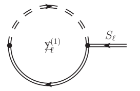
Figure 2: The collision term ${\cal C}_{\ell}^{\rm self}$, Eq. (19).

When all propagators are on shell and massless, $p^{2}=k^{2}=q^{2}=0$, this self energy does not contribute to the collision term, so that no contribution of order $h^{\dagger}h$ arises. However once the medium effects are included by replacing the tree level propagators with resummed propagators, one obtains contributions that are parametrically of order $g^{2}h^{\dagger}h$. The LO terms of this type will be calculated in Section 3.

The vertex-type diagrams give an order $g^{2}h^{\dagger}h$ contribution to the collision term when evaluated using tree-level propagators. While in principle, it would be possible to evaluate also these diagrams with finite temperature resummed propagators, the difference between the two calculations is of higher order in the gauge coupling. For the purpose of the present work, it is therefore sufficient to calculate ${\cal C}_{\ell}^{\rm vertex}$ using tree level propagators, which will be performed in Section 4.

In Ref. [31] it is shown that collinearly enhanced $1\leftrightarrow 2$ processes appear as a third contribution that is parametrically as important as the two contributions discussed above, and which requires a resummation of ladder diagrams with an arbitrary number of soft gauge bosons inserted between the Higgs and the lepton propagator in Figure 1. These multiple scattering contributions will be evaluated in Section 5.

2.4 Flavour Equilibration Rate

The evolution equations for the left- (right-) handed lepton asymmetries $q_{\ell}$ ($q_{R}$) are given by [11]

$$\frac{d}{dt}q_{\ell} =-\left\{W_{\ell},q_{\ell}\right\}+2{\rm S}_{\ell}-\Gamma^{\rm fl}_{\ell}\,,$$ (20a)

$$\frac{d}{dt}q_{{\rm R}} =-\Gamma^{\rm fl}_{\rm R}\,,$$ (20b)

where in general, $q_{\ell,{\rm R}}$ and $W_{\ell}$, ${\rm S}_{\ell}$ and $\Gamma^{\rm fl}_{\ell,{\rm R}}$ are $3\times 3$ matrices in flavour space. The charge densities $q_{\ell,{\rm R}}$ are matrix-valued generalisations of charge densities of left- and right-handed SM leptons, that can thereby also account for flavour coherence. The lepton-number violating washout term is denoted by $W_{\ell}$, the source term for the $CP$-asymmetries by ${\rm S}_{\ell}$, and $\Gamma^{\rm fl}_{\ell,{\rm R}}$ describe the equilibration of lepton number between $\ell$ and ${\rm R}$ as well as the decay of flavour coherence. In the standard scenarios of Leptogenesis, there is no direct source for a charge asymmetry in right-handed leptons $R$ and no direct lepton-number violating coupling that woul induce a washout.

Here we are interested in the flavour equilibration rates $\Gamma^{\rm fl}_{\ell,{\rm R}}$ that depend on the Yukawa couplings $h_{ab}$. The rate $\Gamma^{\rm fl}_{\ell}$ can be obtained by integrating the relevant part of the collision term ${\cal C}_{\ell}$:

$$-\Gamma^{\rm fl}_{\ell} =\frac{1}{2}\int\frac{d^{4}p}{(2\pi)^{4}}{\rm tr}\,{\cal C}^{\rm fl}_{\ell}(p)+{\rm h.c.}=\frac{1}{2}\int\frac{d^{4}p}{(2\pi)^{4}}{\rm tr}\left[{\rm i}{\Sigma\!\!\!/}_{\ell}^{{\rm fl}>}(p){\rm i}S_{\ell}^{<}(p)-{\rm i}{\Sigma\!\!\!/}_{\ell}^{{\rm fl}<}(p){\rm i}S_{\ell}^{>}(p)\right]+{\rm h.c.}$$ (21)

where h.c. denotes hermitian conjugation in flavour space, and the superscript ${\rm fl}$ indicates that we only consider those contributions to the collision term that are at least second order in the charged lepton Yukawas $h_{ab}$.

We assume that the particles $\ell$ and ${\rm R}$ are in kinetic equilibrium, i.e. their distributions are of the Fermi-Dirac form with generalised, matrix-valued chemical potentials $\mu_{\ell,{\rm R}\,ab}$. Moreover, we assume that the chemical potentials are small, $\mu_{\ell,{\rm R}\,ab}\ll T$. We can then expand the collision term to linear order in the chemical potentials using

$$f_{\ell ab}(k) =\frac{1}{e^{\beta k^{0}}+1}\delta_{ab}+\delta f_{\ell ab}(k)\,,$$ (22)

$$\delta f_{\ell ab}(k) =\beta\frac{e^{\beta k^{0}}}{(e^{\beta k^{0}}+1)^{2}}\mu_{\ell ab}\equiv 6\beta^{3}\frac{e^{\beta k^{0}}}{(e^{\beta k^{0}}+1)^{2}}q_{\ell ab}\,.$$ (23)

Note that this also implies a decomposition of the Wigner functions ${\rm i}S_{\ell}^{<,>}={\rm i}S_{\ell,{\rm eq}}^{<,>}+{\rm i}\delta S_{\ell}$, where the deviation from equilibrium is given by

$${\rm i}\delta S_{\ell}=-2S_{\ell}^{\cal A}\delta f_{\ell}(p)\,.$$ (24)

Accordingly, the term linear in the right-handed SM lepton asymmetry $q_{\rm R}$ is obtained by expanding ${\rm i}S_{\rm R}^{<,>}$, which enters $\Gamma^{\rm fl}_{\ell}$ through Eqs. (18) and (21). Now we expand Eq. (21) in $\mu_{\ell,{\rm R}}/T$. Due to the Kubo-Martin-Schwinger (KMS) relations, ${\rm i}S_{\ell,{\rm R},{\rm eq}}^{>}(p)=-{\rm e}^{\beta p^{0}}{\rm i}S_{\ell,{\rm R},{\rm eq}}^{<}(p)$ and ${\rm i}\not{\Sigma}_{\ell,{\rm eq}}^{{\rm fl}>}(p)=-{\rm e}^{\beta p^{0}}{\rm i}\not{\Sigma}_{\ell,{\rm eq}}^{{\rm fl}<}(p)$, where ${\rm i}\not{\Sigma}_{\ell,{\rm eq}}^{\rm fl}$ is the contribution from the equilibrium parts of the individual propagators to the self energy, the leading terms in this expansion are linear in $\mu_{\ell,{\rm R}}$ (i.e. the equilibrium contributions vanish). Therefore, the flavour-sensitive contribution to the lepton collision term takes the general form

$$-\frac{dq_{\ell}}{dt}=\Gamma_{\ell}^{\rm fl}=\frac{\gamma^{{\rm fl}\delta\ell}}{2}\left(h^{\dagger}hq_{\ell}+{\rm h.c.}\right)+\frac{\gamma^{{\rm fl}\delta{\rm R}}}{2}\left(h^{\dagger}q_{\rm R}h+{\rm h.c.}\right),$$ (25)

where we have defined the reduced scattering rates $\gamma^{{\rm fl}\delta\ell,R}$. Due to lepton number conservation of the interactions mediated by $h$ in combination with flavour-blind gauge interactions, we expect that $\gamma^{{\rm fl}\delta\ell}=-\gamma^{{\rm fl}\delta{\rm R}}$, what we explicitly verify in the calculations. Note that $q_{\ell ab}=\delta n^{+}_{\ell ab}-\delta n^{-}_{\ell ab}$ is the difference of the deviations of the lepton and anti-lepton number densities from thermal equilibrium. Fast gauge interactions ensure that [11] $\delta n^{+}_{\ell ab}=-\delta n^{-}_{\ell ab}$ such that $\Gamma^{\rm fl}_{\ell ab}$ can be obtained from the collision term according to Eq. (21), otherwise the collision terms for particles and anti-particles would have to be evaluated separately, and equations of motion for each $\delta n_{\ell ab}^{+}$ and $\delta n_{\ell ab}^{-}$ would have to be solved.

The coefficients $\gamma^{{\rm fl}\delta\ell,\delta{\rm R}}$ have contributions from several diagrams,

$$\gamma^{{\rm fl}\delta\ell,\delta{\rm R}}=\gamma^{{\rm fl}{\rm(A)}\delta\ell,\delta{\rm R}}+\gamma^{{\rm fl}{\rm(B)}\delta\ell,\delta{\rm R}}+\ldots\,,$$ (26)

which we calculate in the following. Likewise, we decompose the self energies $\not{\Sigma}_{\ell}$, the collison terms ${\cal C}_{\ell}^{\rm fl}$ and the damping rates $\Gamma_{\ell}^{\rm fl}$ into various diagrammatic components.

2.5 Right-Handed Neutrino Production Rate

The kinetic equation for the right-handed neutrino density $f_{N_{i}}(\mathbf{p})$ is given by

$$\frac{d}{dt}f_{N_{i}}(\mathbf{p}) =D_{i}(\mathbf{p})\,,$$ (27)

where the decay (or inverse decay) rate $D_{i}$ is obtained by integrating the collision term over $p^{0}$ [19]:

$$D_{i}(\mathbf{p}) =\frac{1}{4}\int\frac{dp^{0}}{2\pi}{\rm sign}(p^{0}){\rm tr}{\cal C}_{Ni}(p)$$ (28)

$$=\frac{1}{4}\int\frac{dp^{0}}{2\pi}{\rm sign}(p^{0}){\rm tr}\left[{\rm i}{\Sigma\!\!\!/}_{Nii}^{>}(p){\rm i}S_{Ni}^{<}(p)-{\rm i}{\Sigma\!\!\!/}_{Nii}^{<}(p){\rm i}S_{Ni}^{>}(p)\right].$$

Here, we neglect the effect of possible off-diagonal correlations in the neutrino propagator. As long as the mass differences $M_{Ni}-M_{Nj}$ are much larger than the relaxation rates $D$, this is a suitable approximation, because the off-diagonal correlations oscillate rapidly and do not give a coherent contribution to the diagonal evolution. In the case of a strong mass-degeneracy, the full evolution of diagonal distributions as well as the oscillatory off-diagonal correlations must be considered, as it is described in Ref. [21]. For simplicity, we suppress in the following the flavour indices for the sterile right-handed neutrinos.

For the right-handed neutrinos, the medium corrections to the propagator are proportional to $|Y|^{2}$ and therefore negligible in general, such that we can use the tree propagators (3) with mass $M_{N}$ in the Wightman functions (2). Inserting these into Eq. (27), the $p^{0}$ integral can be performed analytically, and one obtains (suppressing the flavour indices)

$$\frac{d}{dt}f_{N}(\mathbf{p})=\frac{1}{2\omega(\mathbf{p})}{\rm tr}\left[{p\!\!\!/}{\Sigma\!\!\!/}_{N}^{\cal A}(p)\right]\left(\frac{1}{e^{\beta\omega(\mathbf{p})}+1}(1-f_{N}(\mathbf{p}))-\left(1-\frac{1}{e^{\beta\omega(\mathbf{p})}+1}\right)f_{N}(\mathbf{p})\right),$$ (29)

where $p^{0}=\omega(\mathbf{p})=\sqrt{\mathbf{p}^{2}+M_{N}^{2}}$ and where we have used that $\ell$ and $\phi$ are in thermal equilibrium, such that the self energies satisfy the KMS condition ${\rm i}{\Sigma\!\!\!/}_{N}^{>}(p)=-e^{\beta p^{0}}{\rm i}{\Sigma\!\!\!/}_{N}^{<}(p)$. Furthermore, the spectral part of the self energy is defined as

$${\Sigma\!\!\!/}^{\cal A}=\frac{1}{2}\left({\rm i}{\Sigma\!\!\!/}^{>}-{\rm i}{\Sigma\!\!\!/}^{<}\right).$$ (30)

Taking account of initial conditions for $f_{Ni}$ and of the expansion of the Universe, solving Eq. (29) results in a non-equilibrium distribution function $f_{N}(\mathbf{p})$, which can be computed numerically, but for which no simple analytical form applies in general. Presenting an illustrative result for the neutrino production rate therefore is to some extent a matter of definition. For the ease of comparison, we follow Ref. [31], and choose the production rate for $f_{N}(\mathbf{p})\equiv 0$. Approximately, this is the relevant rate for the production of singlet neutrinos in the weak washout scenario, provided it is assumed that initially, the density of these particles vanishes. The differential production rate for the sum of the two spin orientations is

$$\gamma^{N}=\frac{d\Gamma_{N}}{d^{3}p}=\frac{2}{(2\pi)^{3}}\frac{d}{dt}f_{N}(\mathbf{p})=-\frac{1}{(2\pi)^{3}}\frac{1}{2p^{0}}{\rm tr}[\not{p}{\rm i}\not{\Sigma}_{N}^{<}(p)]\,,$$ (31)

where

$${\rm i}\not{\Sigma}^{<}_{N}(p)=-2\frac{1}{{\rm e}^{\beta p^{0}}+1}\not{\Sigma}_{N}^{\cal A}(p)\,.$$ (32)

To see more explicitly how this rate is related to the flavour relaxation rate defined in the previous section, it is instructive to consider the leptonic collision term ${\cal C}^{\rm fl}_{\ell}(p)$. As before, we expand ${\rm i}S_{\ell}^{<,>}={\rm i}S_{\ell,{\rm eq}}^{<,>}+{\rm i}\delta S_{\ell}$ and recall that ${\rm i}\delta S_{\ell}$ can be approximated as being linear in $q_{\ell}$. To leading order in deviations from equilibrium, we can therefore assume that the self energies satisfy the KMS relation. This part of the collision term then simplifies to

$$\frac{1}{2}\int\frac{dp^{0}}{2\pi}{\rm tr}[{\cal C}^{\rm fl}_{\ell}(p)]=-\frac{1}{|p^{0}|}{\rm tr}[P_{R}{p\!\!\!/}{\Sigma\!\!\!/}^{{\rm fl}\cal A}_{\ell}(p)]\delta f_{\ell}(p^{0})+{\cal O}(\delta f_{R})+{\rm h.c.}\,,$$ (33)

with $p^{0}=\pm|\mathbf{p}|$. This has the same structure as the equation for the differential right-handed neutrino production rate (29) except for the different statistical weight functions. A relation between ${\rm tr}[\not{p}\not{\Sigma}_{N}^{\cal A}]$ and ${\rm tr}[\not{p}\not{\Sigma}_{\ell}^{{\rm fl}\cal A}]$ is obtained by isolating the dependence on the coupling constants. In most cases, these are simple proportionalities, whereas for $t$-channel fermion exchange, there is an additional logarithmic dependence on the gauge couplings which can be isolated as well. Therefore, once the differential (in $|\mathbf{p}|$) flavour relaxation rate is known, the $N$ production and decay rates can be obtained by simply performing the integral with the appropriate statistical weight and a rescaling of the couplings.

3 Self-Energy Type Contributions

3.1 One-Loop Self Energies

The resummed form of the spectral function of a massless chiral fermion is [11, 41, 42]

$$S^{\cal A}(k)=P_{X}\frac{2\left(k\!\!\!/-{\Sigma\!\!\!\!/}^{H}\right)\Sigma^{\cal A}\cdot(k-\Sigma^{H})-{\Sigma\!\!\!\!/}_{\ell}^{\cal A}\left(k\!\!\!/-{\Sigma\!\!\!\!/}^{H}\right)^{2}+{{{{\Sigma\!\!\!\!/}}^{{\cal A}\,3}}}}{\left[\left(k\!\!\!/-{\Sigma\!\!\!\!/}^{H}\right)^{2}-{{\Sigma\!\!\!\!/}^{{\cal A}\,2}}\right]^{2}+4\left[\Sigma^{\cal A}\cdot(k-\Sigma^{H})\right]^{2}}\,,$$ (34)

and of a massless scalar

$$\Delta_{\phi}^{\cal A}(k)=\frac{\Pi^{\cal A}_{\phi}(k)}{k^{4}+[{\Pi^{\cal A}_{\phi}(k)}]^{2}}\,.$$ (35)

We express the spin-$\frac{1}{2}$ fermionic self energies as $\not{\Sigma}=\gamma^{\mu}\Sigma_{\mu}$. In the approximation of massless particles in the loop, the spectral self energy for leptons $\ell$ or ${\rm R}$ is given by

$$\Sigma^{{\cal A}0}_{\ell,{\rm R}}(k) =\frac{GT^{2}}{16\pi|\mathbf{k}|}I_{1}\left({\frac{k^{0}}{T},\frac{|\mathbf{k}|}{T}}\right)\,,$$ (36a)

$$\Sigma^{{\cal A}i}_{\ell,{\rm R}}(k) =\frac{GT^{2}}{16\pi|\mathbf{k}|}\left[\frac{k^{0}}{|\mathbf{k}|}I_{1}\left({\frac{k^{0}}{T},\frac{|\mathbf{k}|}{T}}\right)-\frac{(k^{0})^{2}-\mathbf{k}^{2}}{2|\mathbf{k}|T}I_{0}\left({\frac{k^{0}}{T},\frac{|\mathbf{k}|}{T}}\right)\right]\frac{k^{i}}{|\mathbf{k}|}\,,$$ (36b)

where

$$I_{0}(y^{0},y)= -\vartheta(y^{2}-(y^{0})^{2})y^{0}-y+\log\left|\frac{1+{\rm e}^{\frac{1}{2}(y^{0}+y)}}{1+{\rm e}^{\frac{1}{2}(y^{0}-y)}}\right|+\log\left|\frac{1-{\rm e}^{\frac{1}{2}(y^{0}+y)}}{1-{\rm e}^{\frac{1}{2}(y^{0}-y)}}\right|\,,$$ (37a)

$$I_{1}(y^{0},y)= -\vartheta(y^{2}-(y^{0})^{2})\frac{(y^{0})^{2}-\pi^{2}}{2}$$ (37b)

$$+ {\rm Re}\left[x(\log(1+{\rm e}^{x})-\log(1-{\rm e}^{x-y^{0}}))+{\rm Li}_{2}(-{\rm e}^{x})-{\rm Li}_{2}({\rm e}^{x-y^{0}})\right]^{x=\frac{1}{2}(y^{0}+y)}_{x=\frac{1}{2}(y^{0}-y)}\,.$$

For the case of the Standard Model lepton doublet $\ell$, $G=\frac{1}{2}(3g_{2}^{2}+g_{1}^{2})$, whereas for right-handed leptons ${\rm R}$, $G=2g_{1}^{2}$. Notice that these values for $G$ include a factor of two that accounts for the polarisation states of the gauge bosons, as the spectral self energies (36) are defined here for a single bosonic and a fermionic (with both spin states) degree of freedom in the loop. Note as well that we distinguish between the lepton self energy (36), that is flavour-diagonal and of order $g^{2}$, and the flavour-sensitive self energy ${\rm i}\not{\Sigma}_{\ell}^{\rm fl}$, for which the LO terms are $\sim h^{2}g^{2}$ and $\sim h^{2}g^{2}\log g^{2}$.

The spectral self energy for the Higgs field is given by

$$\Pi^{\cal A}_{\phi}= \frac{\frac{3}{2}g_{2}^{2}+\frac{1}{2}g_{1}^{2}}{16\pi}\frac{k^{2}}{|\mathbf{k}|}\left(|\mathbf{k}|-\frac{2}{\beta}\log\frac{1-{\rm e}^{\beta\frac{k^{0}+|\mathbf{k}|}{2}}}{1-{\rm e}^{\beta\frac{k^{0}-|\mathbf{k}|}{2}}}\right)$$ (38a)

$$- \frac{3h_{t}^{2}}{16\pi}\frac{k^{2}}{|\mathbf{k}|}\left(|\mathbf{k}|-\frac{2}{\beta}\log\frac{1+{\rm e}^{\beta\frac{k^{0}+|\mathbf{k}|}{2}}}{1+{\rm e}^{\beta\frac{k^{0}-|\mathbf{k}|}{2}}}\right)\;\;\textnormal{for}\;\;k^{2}\geq 0\,,$$

$$\Pi^{\cal A}_{\phi}= \frac{\frac{3}{2}g_{2}^{2}+\frac{1}{2}g_{1}^{2}}{16\pi}\frac{k^{2}}{|\mathbf{k}|}\left(2k^{0}-\frac{2}{\beta}\log\frac{1-{\rm e}^{\beta\frac{|\mathbf{k}|+k^{0}}{2}}}{1-{\rm e}^{\beta\frac{|\mathbf{k}|-k^{0}}{2}}}\right)$$ (38b)

$$- \frac{3h_{t}^{2}}{16\pi}\frac{k^{2}}{|\mathbf{k}|}\left(2k^{0}-\frac{2}{\beta}\log\frac{1+{\rm e}^{\beta\frac{|\mathbf{k}|+k^{0}}{2}}}{1+{\rm e}^{\beta\frac{|\mathbf{k}|-k^{0}}{2}}}\right)\;\;\textnormal{for}\;\;k^{2}<0\,.$$

When we substitute tree-level propagators for all three fields $\ell$, ${\rm R}$ and $\phi$ that appear in the expression for ${\cal C}_{\ell}^{\rm self}$ defined by Eqs. (18,19), we obtain a vanishing result, because the $1\leftrightarrow 2$ process is kinematically forbidden (when neglecting the tree-level masses) without including the finite-temperature corrections. At leading order in the gauge and top-quark Yukawa couplings, the medium corrections add linearly such that the one-loop (in the 2PI sense) self energy (18) for the lepton doublet can be approximated as

$${\rm i}\not{\Sigma}_{\ell}^{(1)}(p)\approx{\rm i}\not{\Sigma}_{\ell}^{(\rm R)}(p)+{\rm i}\not{\Sigma}_{\ell}^{(\phi)}(p)\qquad\textnormal{for}\;p^{2}=0\,,$$ (39)

where

$${\rm i}\not{\Sigma}_{\ell}^{({\rm R})ab}(p)= h^{\dagger}\int\frac{d^{4}k}{(2\pi)^{4}}\frac{d^{4}q}{(2\pi)^{4}}(2\pi)^{4}\delta^{4}(p-k-q){\rm i}\Delta_{\phi}^{(0)ab}(k){\rm i}S_{\rm R}^{ab}(q)h\,,$$ (40a)

$${\rm i}\not{\Sigma}_{\ell}^{(\phi)ab}(p)= h^{\dagger}\int\frac{d^{4}k}{(2\pi)^{4}}\frac{d^{4}q}{(2\pi)^{4}}(2\pi)^{4}\delta^{4}(p-k-q){\rm i}\Delta_{\phi}^{ab}(k){\rm i}S_{\rm R}^{(0)ab}(q)h\,,$$ (40b)

$${\rm i}\not{\Sigma}_{\ell}^{({\rm os})ab}(p)= h^{\dagger}\int\frac{d^{4}k}{(2\pi)^{4}}\frac{d^{4}q}{(2\pi)^{4}}(2\pi)^{4}\delta^{4}(p-k-q){\rm i}\Delta_{\phi}^{(0)ab}(k){\rm i}S_{\rm R}^{(0)ab}(q)h\,.$$ (40c)

Here, we have also defined the contribution from on-shell Higgs bosons and right-handed SM leptons ${\rm i}\not{\Sigma}_{\ell}^{({\rm os})ab}(p)$, where ${\rm i}\not{\Sigma}_{\ell}^{({\rm os})<,>}(p)=0$ for $p^{2}=0$ for the kinematic reasons mentioned above. However, since the resummed propagator ${\rm i}S_{\ell}^{<,>}(p)$ is non-vanishing for $p^{2}\not=0$, there occurs a contribution involving ${\rm i}\not{\Sigma}_{\ell}^{({\rm os})ab}(p)$ that is kinematically allowed due to gauge bosons that may radiate from $\ell$.

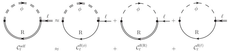
Figure 3: Diagrammatic representation of the LO expansion of the one-loop 2PI collision term, Eq. (41).

In summary, we can decompose the self-energy contributions to the flavour-decohering collision term as

$${\cal C}_{\ell}^{\rm self}\approx{\cal C}_{\ell}^{{\rm fl}(\phi)}+{\cal C}_{\ell}^{{\rm fl}({\rm R})}+{\cal C}_{\ell}^{{\rm fl}(\ell)}\,,$$ (41)

where

$${\cal C}_{\ell}^{{\rm fl}(\phi,{\rm R})}= {\rm tr}\left[{\rm i}\not{\Sigma}_{\ell}^{(\phi,{\rm R})>}(p){\rm i}S_{\ell}^{(0)<}(p)-{\rm i}\not{\Sigma}_{\ell}^{(\phi,{\rm R})<}(p){\rm i}S_{\ell}^{(0)>}(p)\right]\,,$$ (42)

$${\cal C}_{\ell}^{{\rm fl}(\ell)}= {\rm tr}\left[{\rm i}\not{\Sigma}_{\ell}^{({\rm os})>}(p){\rm i}S_{\ell}^{<}(p)-{\rm i}\not{\Sigma}_{\ell}^{({\rm os})<}(p){\rm i}S_{\ell}^{>}(p)\right]\,.$$ (43)

A diagrammatic representation of the decomposition (41) is given by Figure 3.

3.2 Scatterings via the Higgs Boson

Substituting the tree-level spectral function (3) for $\ell$ and ${\rm R}$ and the one-loop resummed spectral function for $\phi$, the collision term becomes

$${\cal C}_{\ell}^{{\rm fl}(\phi)}= \int\frac{d^{4}k}{(2\pi)^{4}}\frac{d^{4}q}{(2\pi)^{4}}(2\pi)^{4}\delta^{4}(p+k-q)\frac{2\Pi_{\phi}^{\cal A}(k)}{k^{4}+[\Pi^{\cal A}_{\phi}(k)]^{2}}2p\cdot q$$ (44)

$$\times 2\pi\delta(p^{2})2\pi\delta(q^{2}){\rm sign}(p^{0}){\rm sign}(q^{0})$$

$$\times h^{\dagger}\left[(1+f_{\phi}(k^{0}))f_{\rm R}(q^{0})h(1-f_{\ell}(p^{0}))-f_{\phi}(k^{0})(1-f_{\rm R}(q^{0}))hf_{\ell}(p^{0})\right]\,.$$

It is now useful to notice that $\Pi^{\cal A}(k)$ is first order in $k^{2}$ for $k^{2}\to 0$ [cf. Eq. (38)], as well as $2p\cdot q=k^{2}$ (due to the relations imposed by the $\delta$-functions). To leading order in the couplings $g^{2}_{1,2}$ and $h_{t}^{2}$, we may therefore replace

$$\frac{2\Pi_{\phi}^{\cal A}}{k^{4}+[\Pi^{\cal A}_{\phi}]^{2}}\approx\frac{2\Pi_{\phi}^{\cal A}}{k^{4}}\,,$$ (45)

such that in this approximation, ${\cal C}_{\ell}^{{\rm fl}(\phi)}$ is proportional to $g^{2}_{1,2}$ and $h_{t}^{2}$. Alternatively, one can derive Eq. (44) with the replacement (45) from a CTP two-loop (two particle reducible) self energy in terms of tree-level propagators.

We now assume that $\phi$, $\ell$, ${\rm R}$ are in kinetic equilibrium, and that the chemical potentials of $\ell$ and ${\rm R}$ are small compared to the temperature, such that we may relate

$$\delta f_{\ell,{\rm R}}(p^{0})=6\beta^{3}\frac{{\rm e}^{\beta p^{0}}}{({\rm e}^{\beta p^{0}}+1)^{2}}q_{\ell,{\rm R}}\,,$$ (46)

where $\delta f_{\ell,{\rm R}}(p^{0})=f_{\ell,{\rm R}}(p^{0})-f_{F}^{\rm eq}(p^{0})$. Note that $\delta f_{\ell,{\rm R}}(p^{0})$ and $q_{\ell,{\rm R}}$ are understood as matrices in flavour space and $f_{F}^{\rm eq}(p^{0})$, the Fermi-Dirac equilibrium distribution for vanishing chemical potential, is therefore implied to be proportional to the unit matrix.

With the definitions (21,25,26), it follows

$$\gamma^{{\rm fl}(\phi)\delta\ell}= -\gamma^{{\rm fl}(\phi)\delta{\rm R}}$$

$$= -\int\frac{d^{4}k}{(2\pi)^{4}}\int\frac{d^{4}p}{(2\pi)^{4}}\int\frac{d^{4}q}{(2\pi)^{4}}(2\pi)^{4}\delta^{4}(p+k-q)\frac{2\Pi^{\cal A}(k)}{k^{2}}2\pi\delta(p^{2})2\pi\delta(q^{2})$$ (47)

$$\times {\rm sign}(p^{0}){\rm sign}(q^{0})\frac{{\rm e}^{\beta k^{0}}+{\rm e}^{\beta q^{0}}}{({\rm e}^{\beta k^{0}}-1)({\rm e}^{\beta q^{0}}+1)}6\beta^{3}\frac{{\rm e}^{\beta p^{0}}}{({\rm e}^{\beta p^{0}}+1)^{2}}$$

$$= 7.71\times 10^{-4}\times\left(\frac{3}{2}g_{2}^{2}+\frac{1}{2}g_{1}^{2}\right)T+1.32\times 10^{-3}\times h_{t}^{2}T\,,$$

where the last expression is the result of numerical evaluation of the integrals.

3.3 Scatterings via Fermions

Now consider the terms that arise from substituting the tree-level spectral function (9) for the scalar propagator and (3) for one of the fermions $\ell$ or ${\rm R}$, while using the resummed spectral function (34) for the other fermion. For definiteness, we calculate the collison term for scatterings via ${\rm R}$ first [i.e. with ${\rm i}S_{\rm R}^{\cal A}$ as in Eq. (34)]:

$${\cal C}_{\ell}^{{\rm fl}({\rm R})}(p)= \int\frac{d^{4}k}{(2\pi)^{4}}\frac{d^{4}q}{(2\pi)^{4}}(2\pi)^{4}\delta^{4}(p-k+q)2{\rm tr}\left[S_{\rm R}^{\cal A}(k)\not{p}\right]$$ (48)

$$\times 2\pi\delta(p^{2})2\pi\delta(q^{2}){\rm sign}(p^{0}){\rm sign}(q^{0})$$

$$\times \left[h^{\dagger}f_{\rm R}(k^{0})h(1-f_{\ell}(p^{0}))(1+f_{\phi}(q^{0}))-h^{\dagger}(1-f_{\rm R}(q^{0}))hf_{\ell}(p^{0})f_{\phi}(q^{0})\right]\,.$$

The contribution from scatterings via $\ell$ can directly be inferred from the evaluation of this term. Expanding in the deviations of $f_{\ell,{\rm R}}$ from chemical equilibrium, we write

$${\cal F}(k^{0},p^{0},q^{0})= \left[h^{\dagger}f_{\rm R}(k^{0})h(1-f_{\ell}(p^{0}))(1+f_{\phi}(q^{0}))-h^{\dagger}(1-f_{\rm R}(q^{0}))hf_{\ell}(p^{0})f_{\phi}(q^{0})\right]$$ (49)

$$= -h^{\dagger}h\delta f_{\ell}(p^{0})\left[\frac{1}{{\rm e}^{\beta k^{0}}+1}+\frac{1}{{\rm e}^{\beta q^{0}}-1}\right]$$

$$+ h^{\dagger}\delta f_{\rm R}(k^{0})h\left[1-\frac{1}{{\rm e}^{\beta p^{0}}+1}+\frac{1}{{\rm e}^{\beta q^{0}}-1}\right]\,,$$

what leads to the decomposition ${\cal C}_{\ell}^{{\rm fl}({\rm R})}={\cal C}_{\ell}^{{\rm fl}({\rm R})\delta\ell}+{\cal C}_{\ell}^{{\rm fl}({\rm R})\delta{\rm R}}$ and accordingly for $\Gamma^{\rm fl}$ and $\gamma^{\rm fl}$.

The collision term (48) can straightforwardly be evaluated numerically. After making use of the $\delta$-functions, homogeneity and isotropy, two numerical integrations are left. However, it is useful and instructive to isolate the dependence on the coupling $G$.

It is known that the phase space integrals over the scattering matrix elements exhibit a logarithmic divergence for zero-momentum exchange of a lepton ${\rm R}$ in the $t$ channel. The scattering approximation is recovered in the present approach when omitting the self energies in the denominator of the spectral function, Eq. (34), which would lead to a logarithmic divergence in the integral (48) for $k^{0}=|\mathbf{k}|=0$ and $k^{2}<0$. A simplification corresponding to the replacement (45) is therefore not suitable for the present integral. A finite part can however be extracted when subtracting those terms from the spectral self energy $\not{\Sigma}^{\cal A}_{\rm R}$ that are not vanishing in the limit $k^{0},|\mathbf{k}|\to 0$. These are precisely the contributions that are of the form of the hard thermal loop (HTL) approximation and that we indicate by a tilde. We therefore define

$$\bar{I}_{1}(y^{0},y) =I_{1}(y^{0},y)-\tilde{I}_{1}(y^{0},y)\,,$$ (50)

$$\tilde{I}_{1}(y^{0},y) =\vartheta(y^{2}-(y^{0})^{2})\frac{\pi^{2}}{2}\,.$$ (51)

The barred quantities $\bar{S}^{\cal A}$ and $\bar{\Sigma}$ are defined through the replacement $I_{1}\to\bar{I}_{1}$, and accordingly $\Sigma^{\cal A}=\bar{\Sigma}^{\cal A}+\tilde{\Sigma}^{{\cal A}}$, ${\cal C}_{\ell}^{{\rm fl}{\rm(R)}}=\bar{\cal C}_{\ell}^{{\rm fl}{\rm(R)}}+\tilde{\cal C}_{\ell}^{{\rm fl}{\rm(R)}}$. Note that $I_{0}$ vanishes in the HTL approximation.

For the purpose of calculating $\bar{\cal C}_{\ell}^{{\rm fl}{\rm(R)}}$ to leading order in $G$, it is sufficient to approximate

$$\bar{S}_{\rm R}^{\cal A}(k)=P_{\rm R}\frac{2k\!\!\!/\bar{\Sigma}_{\rm R}^{\cal A}\cdot k-\bar{\Sigma\!\!\!\!/}_{\rm R}^{\cal A}k^{2}}{k^{4}}P_{\rm L}\,.$$ (52)

The result for $\bar{\cal C}_{\ell}^{{\rm fl}{\rm(R)}}$ is therefore manifestly proportional to $G$.

It remains to calculate the part that originates from the term of the HTL form. Therefore, we need to find

$$\tilde{\cal C}_{\ell}^{{\rm fl}{\rm(R)}}(p)= 2\pi\delta(p^{2}){\rm sign}(p^{0})\int\frac{d^{4}k}{(2\pi)^{4}}\frac{d^{4}q}{(2\pi)^{4}}(2\pi)^{4}\delta(p-k+q)2\pi\delta(q^{2}){\rm sign}(q^{0})$$ (53)

$$\times 2{\rm tr}\left[\not{p}P_{\rm R}\frac{2(\not{k}-\not{\Sigma}_{\rm R}^{H})\tilde{\Sigma}_{\rm R}^{\cal A}\cdot(k-\Sigma_{\rm R}^{H})-\tilde{\not{\Sigma}}_{\rm R}^{\cal A}\left(\not{k}-\not{\Sigma}_{\rm R}^{H}\right)^{2}+{\tilde{\not{\Sigma}}_{\rm R}^{\cal A}{}}^{3}}{\left[\left(\not{k}-\not{\Sigma}_{\rm R}^{H}\right)^{2}-{{{\tilde{\not{\Sigma}}}_{\rm R}^{\cal A}}{}}^{2}\right]^{2}+4\left[\tilde{\Sigma}^{\cal A}\cdot(k-\Sigma^{H})\right]^{2}}\right]\times{\cal F}(k^{0},p^{0},q^{0})\,.$$

In order to extract the dependence on $G$, it is useful to split the integral in a region where $|\mathbf{k}|\geq k_{*}\gg\sqrt{G}T$, where the denominator simplifies (because the self energies may be neglected there far from the single-particle poles) and a region where $|\mathbf{k}|\leq k_{*}\ll|\mathbf{p}|$, where the angular integration simplifies, $\tilde{\cal C}_{\ell}^{{\rm fl}{\rm(R)}}(p)=\tilde{\cal C}_{\ell,<k_{*}}^{{\rm fl}{\rm(R)}}(p)+\tilde{\cal C}_{\ell,>k_{*}}^{{\rm fl}{\rm(R)}}(p)$. Notice that as a consequence of this split, the result should only be valid when $|\mathbf{p}|\gg\sqrt{GT}$. Due to the phase space suppression, this does however not spoil the LO calculation of the flavour relaxation rate.

Dropping the terms $\propto G$ in the denominator, we evaluate

$$\tilde{\cal C}^{{\rm fl}{\rm(R)}}_{\ell,>k_{*}}(p) \underset{p^{0}=|\mathbf{p}|}{=}\frac{GT^{2}}{2^{7}\pi}2\pi\delta(p^{2})\int\limits_{-1}^{1}d\cos\vartheta\int\limits_{k_{*}}^{\infty}\frac{d|\mathbf{k}|}{|\mathbf{k}|}\frac{k^{0}-2|\mathbf{p}|}{|\mathbf{p}|-k^{0}}{\cal F}(k^{0},p^{0},k^{0}-p^{0})\,,$$ (54)

where

$$k^{0}=|\mathbf{p}|-\sqrt{\mathbf{p}^{2}+\mathbf{k}^{2}-2|\mathbf{p}||\mathbf{k}|\cos\vartheta}\,.$$ (55)

(Note that the HTL contributions are only present for $k^{2}<0$.) The collision term for $p^{0}<0$ may be obtained when noting that it is even in $p^{0}$, provided the particle distributions are in kinetic equilibrium.

The logarithmic dependence can be isolated through integration by parts. We simplify the angular integration and additional terms using $k_{*}\ll|\mathbf{p}|$, such that $k^{0}\approx|\mathbf{k}|\cos\vartheta$, and obtain

$$\tilde{\cal C}^{{\rm fl}{\rm(R)}}_{\ell,>k_{*}} =\tilde{\cal C}^{{\rm fl}{\rm(R)}}_{\ell,>k_{*}{\rm LOG}}+\tilde{\cal C}^{{\rm fl}{\rm(R)}}_{\ell,>k_{*}{\rm FIN}}\,,$$ (56a)

$$\tilde{\cal C}^{{\rm fl}{\rm(R)}}_{\ell,>k_{*}{\rm LOG}} =\frac{GT^{2}}{2^{5}\pi}2\pi\delta(p^{2})\log(\beta k_{*}){\cal F}(0,p^{0},-p^{0})\,,$$ (56b)

$$\tilde{\cal C}^{{\rm fl}{\rm(R)}}_{\ell,>k_{*}{\rm FIN}} =\frac{GT^{2}}{2^{7}\pi}2\pi\delta(p^{2})\int\limits_{-1}^{1}d\cos\vartheta\int\limits_{k_{*}}^{\infty}d|\mathbf{k}|\log(\beta|\mathbf{k}|)\frac{\partial}{\partial(\beta|\mathbf{k}|)}\frac{k^{0}-2|\mathbf{p}|}{k^{0}-|\mathbf{p}|}{\cal F}(k^{0},p^{0},k^{0}-p^{0})\,,$$ (56c)

which we have separated into a contribution $\tilde{\cal C}^{{\rm fl}{\rm(R)}}_{\ell,>k_{*}{\rm LOG}}$ that depends logarithmically on $k_{*}$ and an integral $\tilde{\cal C}^{{\rm fl}{\rm(R)}}_{\ell,>k_{*}{\rm FIN}}$ that depends only linearly on $k_{*}$ (i.e. that is finite for $k_{*}\to 0$), such that we can take the lower bound of the integration to zero when $k_{*}\ll|\mathbf{p}|$.

In order to calculate ${\cal I}_{<p_{*}}$, it is necessary to take account of the screening that is induced by the self energies. In addition to the spectral self energy, also the hermitian part is of importance. Because $p_{*}\ll T$, it is sufficient to consider the HTL approximations

$$\Sigma^{H0}(k) =\frac{GT^{2}}{32|\mathbf{k}|}\log\left|\frac{k^{0}+|\mathbf{k}|}{k^{0}-|\mathbf{k}|}\right|\,,$$ (57a)

$$\Sigma^{Hi}(k) =\frac{GT^{2}k^{0}k^{i}}{32|\mathbf{k}|^{3}}\log\left|\frac{k^{0}+|\mathbf{k}|}{k^{0}-|\mathbf{k}|}\right|-\frac{GT^{2}k^{i}}{16\mathbf{k}^{2}}\,.$$ (57b)

We approximate $|\mathbf{p}-\mathbf{k}|=|\mathbf{p}|-\hat{\mathbf{p}}\cdot\mathbf{k}$, and moreover, we evaluate the statistical functions for $k^{0}=|\mathbf{k}|\approx 0$, as it is appropriate for $k_{*}\ll|\mathbf{p}|$. Numerically, we can then obtain the value of

$$\tilde{\cal C}^{\prime{\rm fl}{\rm(R)}}_{\ell,<k_{*}^{\prime}}=-2\pi\delta(p^{2})\frac{{\cal F}(0,p^{0},-p^{0})}{(2\pi)^{2}|\mathbf{p}|}\int\limits_{-1}^{1}d\cos\vartheta\int\limits_{0}^{k^{\prime}_{*}}\mathbf{k}^{2}d|\mathbf{k}|{\rm tr}\left[\not{p}\tilde{S}_{\rm R}^{\prime{\cal A}}(k)\right]\,.$$ (58)

The prime on $\tilde{S}_{\rm R}^{\prime{\cal A}}(k)$ indicates that we evaluate this expression by replacing $G\to G^{\prime}$, and the tilde indicates, that we use the HTL approximation. Above expression then corresponds to the infrared contribution to the scattering rates that arises from a UV cutoff $k_{*}^{\prime}$ and a squared coupling $G^{\prime}$. From the dependence of the HTL self energies on $G$ and on the four-momentum, we observe that a simultaneous rescaling of the squared coupling by a factor of $G/G^{\prime}$ and of the momentum by $\sqrt{G/G^{\prime}}$ rescales the value of the integrand (including the integration measure) by an overall factor of $G/G^{\prime}$. Therefore, $(G/G^{\prime})\tilde{\cal C}^{\prime{\rm fl}({\rm R})}_{<k_{*}^{\prime}}$ also describes scatterings for a squared coupling $G$ and a UV cutoff $\sqrt{G/G^{\prime}}k_{*}^{\prime}$. In order to obtain the contribution for a cutoff $k_{*}$, we must add the integral

$$\tilde{\cal C}^{{\rm fl}{\rm(R)}}_{\ell[\sqrt{G/G^{\prime}}k_{*}^{\prime},k_{*}]} =-2\pi\delta(p^{2})\frac{{\cal F}(0,p^{0},-p^{0})}{(2\pi)^{2}|\mathbf{p}|}\int\limits_{-1}^{1}d\cos\vartheta\int\limits_{\sqrt{G/G^{\prime}}k_{*}^{\prime}}^{k_{*}}\mathbf{k}^{2}d|\mathbf{k}|{\rm tr}\left[\not{p}\tilde{S}_{\rm R}^{{\cal A}}(k)\right]$$ (59)

$$=-2\pi\delta(p^{2})\frac{GT^{2}}{2^{6}\pi}{\cal F}(0,p^{0},-p^{0})\log\left(\frac{G^{\prime}k_{*}^{2}}{G{k_{*}^{\prime}}^{2}}\right)\,.$$

In summary, the wave-function contribution to the scattering rate can be decomposed as

$${\cal C}^{{\rm fl}{\rm(R)}}_{\ell}=\bar{\cal C}^{{\rm fl}{\rm(R)}}_{\ell}+\tilde{\cal C}^{{\rm fl}{\rm(R)}}_{\ell,>k_{*}{\rm LOG}}+\tilde{\cal C}^{{\rm fl}{\rm(R)}}_{\ell,>k_{*}{\rm FIN}}+\tilde{\cal C}^{{\rm fl}{\rm(R)}}_{\ell[\sqrt{G/G^{\prime}}k_{*}^{\prime},k_{*}]}+\frac{G}{G^{\prime}}\tilde{\cal C}^{\prime{\rm fl}{\rm(R)}}_{\ell,<k^{\prime}_{*}}\,.$$ (60)

The terms $\bar{\cal C}^{{\rm fl}{\rm(R)}}_{\ell}$, $\tilde{\cal C}^{{\rm fl}{\rm(R)}}_{\ell,>k_{*}{\rm FIN}}$ and $\frac{G}{G^{\prime}}\tilde{\cal C}^{\prime{\rm fl}{\rm(R)}}_{\ell,<k^{\prime}_{*}}$ should be evaluated numerically and are proportional to $G$. The logarithmic dependence on $G$, that results from the screening of scattering processes with small momentum exchange is isolated in

$$\tilde{\cal C}^{{\rm fl}{\rm(R)}}_{\ell,>k_{*}{\rm LOG}}+\tilde{\cal C}^{{\rm fl}{\rm(R)}}_{\ell[\sqrt{G/G^{\prime}}k_{*}^{\prime},k_{*}]}=2\pi\delta(p^{2})\frac{GT^{2}}{2^{6}\pi}\log\left(\frac{G}{G^{\prime}}\beta^{2}{k_{*}^{\prime}}^{2}\right){\cal F}(0,p^{0},-p^{0})\,.$$ (61)

We emphasise that the final result ${\cal C}^{{\rm fl}{\rm(R)}}_{\ell}$ is by construction independent on the choice of $k_{*}$, $k_{*}^{\prime}$ and $G^{\prime}$, as the dependence of above expression on these parameters is compensated by $\frac{G}{G^{\prime}}\tilde{\cal C}^{\prime{\rm fl}{\rm(R)}}_{\ell,<k^{\prime}_{*}}$. Recall that this approximate cancellation of the dependence on $k_{*}$, $k_{*}^{\prime}$ and $G^{\prime}$ is a consequence of the approximate behaviour of the integrand when $G\sqrt{T}\ll|\mathbf{k}|\ll|\mathbf{p}|$. Below, we verify this numerically in order to test the accuracy of the approximations.

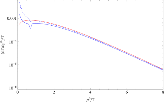
Figure 4: ${\cal C}^{{\rm fl}{\rm(R)}}_{\ell}(p)p^{0}/(\delta q_{\ell})2\pi\delta(p^{2})$ for $\delta q_{\rm R}=0$ over $p^{0}=|\mathbf{p}|$ ($p^{2}=0$) for $G=0.3$. Blue: semi-analytical, Eq (60). Red: full integral. Blue, dashed: semi-analytical without the approximation (52).

Scatterings may as well proceed via the exchange of a doublet lepton $\ell$. This contribution to the collision term is ${\cal C}_{\ell}^{{\rm fl}({\ell})}(p)$, Eq. (42). With the integration over $d^{4}p$, the relevant integrals are identical to those for the exchange of ${\rm R}$. From the result for the scattering via ${\rm R}$, we can therefore directly infer the contribution from exchanges of $\ell$.

Substituting the collision term ${\cal C}^{{\rm fl}{\rm(R)}}_{\ell}$ into the expression for the relaxation rate (25) and using the definition (21), we find

$$\gamma^{{\rm fl}({\rm R},\ell)\delta\ell}=-\gamma^{{\rm fl}({\rm R},\ell)\delta{\rm R}}=4.40\times 10^{-3}\times GT-9.33\times 10^{-4}\times GT\log G\,,$$ (62)

where $G=2g_{1}^{2}$ for ${\rm R}$ exchange (superscript $({\rm R})$) and $G=\frac{3}{2}g_{2}^{2}+\frac{1}{2}g_{1}^{2}$ for $\ell$ exchange (superscript $(\ell)$). Notice that there is an analytical expression for the numerical coefficient of the contribution that is logarithmic in the coupling constant,

$$\int\frac{d^{4}p}{(2\pi)^{4}}2\pi\delta(p^{2}){\rm sign}(p^{0})\frac{T^{2}}{2^{6}\pi}\left(\frac{1}{2}+\frac{1}{{\rm e}^{-\beta p^{0}}-1}\right)\frac{6\beta^{3}{\rm e}^{\beta p^{0}}}{\left({\rm e}^{\beta p^{0}}+1\right)^{2}}=\frac{3}{2^{10}\pi}T\approx 9.33\times 10^{-4}T\,.$$ (63)

The independence of the result (39) on $G$ and $k_{*}$ is valid up to order $G\log G$. The next-to leading expressions are of order $G^{2}\log G$, such that for values of $G\sim 0.3$, one should expect to yield an accuracy of about 20%, which is obviously less than what is suggested by the number of digits given in the numerical coefficients. Note that this estimate for the accuracy is very crude as it does not account for loop and phase-space factors. An estimate of the next-to-leading order (NLO) contribution is non-trivial, and a calculation of the NLO production rate of photons from the quark-gluon plasma has recently been reported in Ref. [43].

We can also extract the coefficients of the contributions that are linear and logarithmic in the couplings by directly performing the integral (48) for different values of the coupling. By this numerical fitting procedure, we find

$$\gamma^{{\rm fl(R,\ell)}\delta\ell}=3.72\times 10^{-3}\times GT-8.31\times 10^{-4}\times GT\log G\,.$$ (64)

This decomposition is valid for a range of $G$ between $G=0.01$ and $G=0.6$ and can therefore also be used for the calculation of related processes in other Baryogenesis scenarios. The numerical difference between the results (62) and (64) is due to a partial inclusion of higher order effects that is implied when (48) is integrated directly.

In Figure 4, we show a comparison of the result from the numerical integration for ${\cal C}^{{\rm fl}{\rm(R)}}_{\ell}(p)$ and the semi-analytic result Eq. (60). There is a very good agreement for large $p^{0}/T$, while we observe the anticipated breakdown of the approximations when $p^{0}=|\mathbf{p}|\gg\sqrt{GT}$ is not valid.

We finally note that in the case of right-handed neutrino production, there is no $t$-channel divergence from the exchange of a left-handed SM-lepton $\ell$ when $M_{N}\not=0$. Rather, this contribution has a logarithmic divergence in $M_{N}^{2}$, as shown in Ref. [40], indicating that the resummed propagator for $\ell$ should be used as well when $M_{N}\not=0$ but $M_{N}\ll T$.

4 Vertex Type Contributions

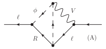
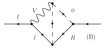
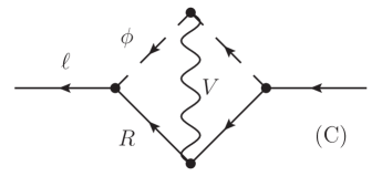
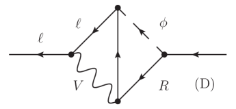
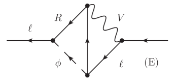
Figure 5: Two-loop self energies that contribute to the flavour relaxation rate, where $V$ stands for both SU(2) and U(1) gauge bosons. Only (A) and (B) are allowed for SU(2) gauge bosons, but all five diagrams appear with U(1) gauge bosons. In the present approximation, we use tree-level propagators, as indicated by the use of single lines, and the external legs are understood to be amputated.

The two-loop self energies that involve two charged lepton Yukawa couplings and that descend from 2PI vacuum graphs are shown in Figure 5. All diagrams are obtained from the one-loop self energy by connecting two different propagators with a gauge boson propagator. Note that diagrams (C), (D), and (E) only exist for the weak hypercharge gauge boson and therefore are of order $g_{1}^{2}h^{2}$.

Since we consider massless particles, virtual corrections to the vertices do not alter the fact that $1\leftrightarrow 2$ processes are kinematically forbidden. Therefore, we can restrict the discussion to those configurations that contribute to the $2\leftrightarrow 2$ scattering rates. Each diagram has two such contributions that are indicated by the cuts in Figure 6.

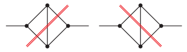
Figure 6: The cuts in the vertex diagrams (indicated by red double lines) that correspond to scatterings. Note that the remaining possible cuts correspond to virtual corrections to $1\leftrightarrow 2$ processes, that are kinematically forbidden for the (approximately) massless particles considered here.

In order to present our calculational method, we discuss in the following the contributions that arise from diagram (C). The approach to calculating the remaining diagrams is very similar and therefore presented more briefly. As we do not need to use resummed propagators for the calculation of the LO contributions from the vertex diagrams, all propagators that are explicitly employed in this Section are understood to be tree-level. For notational simplicity, we omit the superscript $(0)$ that would otherwise occur in a large number of instances. The contribution to the CTP self energy represented in diagram (C) is

$${\rm i}\not{\Sigma}_{\ell}^{{\rm(C)}ab}= Y_{\rm R}Y_{\phi}g_{1}^{2}h^{\dagger}\int\frac{d^{4}k}{(2\pi)^{4}}\int\frac{d^{4}q}{(2\pi)^{4}}\sum\limits_{c,d}cd\,{\rm i}S_{\rm R}^{ac}(k)\gamma^{\mu}{\rm i}\Delta_{\mu\nu}^{cd}(k+q-p)[k-p-q]^{\nu}$$

$$\hskip 113.81102pt\times{\rm i}S_{\rm R}^{cb}(p-q){\rm i}\Delta_{\phi}^{db}(q){\rm i}\Delta_{\phi}^{ad}(p-k)h\,,$$ (65)

where $Y_{\rm R}=-1$ and $Y_{\phi}=\frac{1}{2}$. The collision term only depends on ${\rm i}\Sigma\!\!\!/^{<,>}$. We therefore consider

$${\rm i}\not{\Sigma}_{\ell}^{{\rm(C)}>}(p)= Y_{\rm R}Y_{\phi}g_{1}^{2}\,h^{\dagger}\int\frac{d^{4}k}{(2\pi)^{4}}\int\frac{d^{4}q}{(2\pi)^{4}}$$

$$\bigg{\{} {\rm i}S_{\rm R}^{--}(k)\gamma^{\mu}{\rm i}S_{\rm R}^{-+}(p-q){\rm i}\Delta_{\phi}^{-+}(q)[k-p-q]^{\nu}{\rm i}\Delta_{\phi}^{--}(p-k){\rm i}\Delta^{--}_{\mu\nu}(k+q-p)$$

$$- {\rm i}S_{\rm R}^{-+}(k)\gamma^{\mu}{\rm i}S_{\rm R}^{++}(p-q){\rm i}\Delta_{\phi}^{-+}(q)[k-p-q]^{\nu}{\rm i}\Delta_{\phi}^{--}(p-k){\rm i}\Delta^{+-}_{\mu\nu}(k+q-p)$$

$$- {\rm i}S_{\rm R}^{--}(k)\gamma^{\mu}{\rm i}S_{\rm R}^{-+}(p-q){\rm i}\Delta_{\phi}^{++}(q)[k-p-q]^{\nu}{\rm i}\Delta_{\phi}^{-+}(p-k){\rm i}\Delta^{-+}_{\mu\nu}(k+q-p)$$

$$+ {\rm i}S_{\rm R}^{-+}(k)\gamma^{\mu}{\rm i}S_{\rm R}^{++}(p-q){\rm i}\Delta_{\phi}^{++}(q)[k-p-q]^{\nu}{\rm i}\Delta_{\phi}^{-+}(p-k){\rm i}\Delta^{++}_{\mu\nu}(k+q-p)\bigg{\}}$$

$$\times h\,.$$ (66)

It is useful to shift the momenta in the first and the third term, such that

$${\rm i}\not{\Sigma}_{\ell}^{{\rm(C)}>}(p)= Y_{\rm R}Y_{\phi}g_{1}^{2}h^{\dagger}\int\frac{d^{4}k}{(2\pi)^{4}}\int\frac{d^{4}q}{(2\pi)^{4}}$$

$$\bigg{\{} {\rm i}S_{\rm R}^{--}(p-q)\gamma^{\mu}{\rm i}S_{\rm R}^{-+}(k){\rm i}\Delta_{\phi}^{-+}(p-k)[k-p-q]^{\nu}{\rm i}\Delta_{\phi}^{--}(q){\rm i}\Delta^{--}_{\mu\nu}(k+q-p)$$

$$- {\rm i}S_{\rm R}^{-+}(k)\gamma^{\mu}{\rm i}S_{\rm R}^{++}(p-q){\rm i}\Delta_{\phi}^{-+}(q)[k-p-q]^{\nu}{\rm i}\Delta_{\phi}^{--}(p-k){\rm i}\Delta^{+-}_{\mu\nu}(k+q-p)$$

$$- {\rm i}S_{\rm R}^{--}(p-q)\gamma^{\mu}{\rm i}S_{\rm R}^{-+}(k){\rm i}\Delta_{\phi}^{++}(p-k)[k-p-q]^{\nu}{\rm i}\Delta_{\phi}^{-+}(q){\rm i}\Delta^{+-}_{\mu\nu}(k+q-p)$$

$$+ {\rm i}S_{\rm R}^{-+}(k)\gamma^{\mu}{\rm i}S_{\rm R}^{++}(p-q){\rm i}\Delta_{\phi}^{++}(q)[k-p-q]^{\nu}{\rm i}\Delta_{\phi}^{-+}(p-k){\rm i}\Delta^{++}_{\mu\nu}(k+q-p)\bigg{\}}$$

$$\times h\,.$$ (67)

In the collision term, the Dirac structure of $i\Sigma\!\!\!/_{\ell}^{<,>}(p)$ is dotted into the lepton propagator $iS_{\ell}^{>,<}(p)$, which provides a factor $p\!\!\!/$. Taking the trace over Dirac indices and using that ${\rm tr}[\gamma^{\mu}\gamma^{\nu}\gamma^{\rho}\gamma^{\sigma}]={\rm tr}[\gamma^{\sigma}\gamma^{\rho}\gamma^{\nu}\gamma^{\mu}]$, as well as the cyclicity of the trace, we arrive at the form

$${\rm i}\,{\rm tr} [\not{p}\not{\Sigma}_{\ell}^{{\rm(C)}>}(p)]=Y_{\rm R}Y_{\phi}g_{1}^{2}h^{\dagger}\int\frac{d^{4}k}{(2\pi)^{4}}\int\frac{d^{4}q}{(2\pi)^{4}}{\rm tr}\bigg{[}\not{p}$$

$$\times\bigg{\{} {\rm i}S_{\rm R}^{--}(p-q)\gamma^{\mu}{\rm i}S_{\rm R}^{-+}(k){\rm i}\Delta_{\phi}^{-+}(p-k)[k-p-q]^{\nu}{\rm i}\Delta_{\phi}^{--}(q){\rm i}\Delta^{A--}_{\mu\nu}(k+q-p)$$

$$- {\rm i}S_{\rm R}^{++}(p-q)\gamma^{\mu}{\rm i}S_{\rm R}^{-+}(k){\rm i}\Delta_{\phi}^{--}(p-k)[k-p-q]^{\nu}{\rm i}\Delta_{\phi}^{-+}(q){\rm i}\Delta^{A+-}_{\mu\nu}(k+q-p)$$

$$- {\rm i}S_{\rm R}^{--}(p-q)\gamma^{\mu}{\rm i}S_{\rm R}^{-+}(k){\rm i}\Delta_{\phi}^{++}(p-k)[k-p-q]^{\nu}{\rm i}\Delta_{\phi}^{-+}(q){\rm i}\Delta^{A+-}_{\mu\nu}(k+q-p)$$

$$+ {\rm i}S_{\rm R}^{++}(p-q)\gamma^{\mu}{\rm i}S_{\rm R}^{-+}(k){\rm i}\Delta_{\phi}^{-+}(p-k)[k-p-q]^{\nu}{\rm i}\Delta_{\phi}^{++}(q){\rm i}\Delta^{A++}_{\mu\nu}(k+q-p)\bigg{\}}\bigg{]}$$

$$\times h\,.$$ (68)

First note that it is not possible to put all five propagators simultaneously on shell. Now suppose that $p-q$ is off shell, whereas the remaining momenta are on shell. Then, the second and third term cancel, as well as the first and the fourth. Note that this corresponds to the kinematic regime of the $CP$-violating source of the corresponding diagram for Leptogenesis [11], where the cancellation does not occur in general, because of the complex conjugation of coupling constants.

When three momenta are on shell, the first and the fourth term give a virtual correction to the kinematically suppressed $1\leftrightarrow 2$ process. The $2\leftrightarrow 2$ scatterings are encapsulated within the second and the third term, where the two off-shell momenta are $p-q$ and $k-p$. The numerator algebra of the self energy (4) is given by

$${\rm tr}[\not{p}(\not{p}-\not{q})(\not{k}-\not{p}-\not{q})\not{k}]=8p\cdot k\,p\cdot q-4p^{2}k\cdot(p+2q)\,.$$ (69)

Here, we have used the on-shell conditions $k^{2}=q^{2}=(p-k-q)^{2}=0$, that apply for the second and the third term, while we yet allow for $p^{2}\not=0$, such that this result may be used for the application of calculating the production rate of massive right-handed neutrinos [40]. In what follows however, we set $p^{2}=0$. This leads to the great simplification that the zeros in the numerator and denominator cancel:

$$\frac{1}{2}{\rm tr}[\not{p}(\not{p}-\not{q})(\not{k}-\not{p}-\not{q})\not{k}]\underset{p^{2}=0}{=}(p-q)^{2}(k-p)^{2}\,.$$ (70)

A consequence of the fact that this cancellation does not occur for $p^{2}\not=0$ is the presence of soft and collinear divergences in the particular real and virtual contributions to the vertex-type self energy for the production of massive neutrinos. It is shown in Refs. [38, 39, 40] that upon summation of all contributions, these soft and collinear divergences cancel.

The same discussion can be repeated for $\not{\Sigma}^{{\rm(C)}<}_{\ell}$ by simply exchanging the first and the second CTP index on all propagators. For the integrated collision term, we then obtain

$$\int\frac{d^{4}p}{(2\pi)^{4}}{\cal C}^{\rm fl(C)}_{\ell}= -Y_{\rm R}Y_{\phi}g_{1}^{2}\int\frac{d^{4}p}{(2\pi)^{4}}\int\frac{d^{4}k}{(2\pi)^{4}}\int\frac{d^{4}q}{(2\pi)^{4}}2\pi\delta(p^{2})2\pi\delta(k^{2})2\pi\delta(q^{2})$$ (71a)

$$\times 2\pi\delta((k+q-p)^{2}){\rm sign}(p^{0})\,{\rm sign}(k^{0})\,{\rm sign}(q^{0})\,{\rm sign}(k^{0}+q^{0}-p^{0})$$

$$\times {\cal G}(q^{0},k^{0}+q^{0}-p^{0},k^{0},p^{0})\,,$$

$${\cal G}(E_{1},E_{2} ,E_{3},E_{4})=(1+f_{\phi}(E_{1}))f_{A}(E_{2})h^{\dagger}(1-f_{\rm R}(E_{3}))hf_{\ell}(E_{4})$$ (71b)

$$\qquad\qquad-f_{\phi}(E_{1})(1+f_{A}(E_{2}))h^{\dagger}f_{\rm R}(E_{3})h(1-f_{\ell}(E_{4}))\,.$$

Using the definition (21), we obtain the flavour-sensitive rate

$$\Gamma_{\ell}^{{\rm fl}{\rm(C)}}= Y_{\rm R}Y_{\phi}g_{1}^{2}\int\frac{d^{4}p}{(2\pi)^{4}}\int\frac{d^{4}k}{(2\pi)^{4}}\int\frac{d^{4}q}{(2\pi)^{4}}2\pi\delta(p^{2})2\pi\delta(k^{2})2\pi\delta(q^{2})2\pi\delta((k+q-p)^{2})$$

$$\times {\rm sign}(p^{0})\,{\rm sign}(k^{0})\,{\rm sign}(q^{0})\,{\rm sign}(k^{0}+q^{0}-p^{0})$$

$$\times \frac{1}{2}\left({\cal G}(q^{0},k^{0}+q^{0}-p^{0},k^{0},p^{0})+{\rm h.c.}\right),$$ (71c)

where the hermitian conjugation acts on the implicit flavour indices in ${\cal G}$. In order to extract the coefficients $\gamma^{{\rm fl}{\rm(C)}\delta\ell,\delta{\rm R}}$, we linearise in the chemical potentials for $\ell$ and ${\rm R}$. Since ${\cal G}$ is odd under a simultaneous exchange of $E_{1,3}\leftrightarrow E_{2,4}$ and $\phi,\ell\leftrightarrow A,{\rm R}$, we can do this calculation for $\mu_{\ell}$ and directly infer the result for $\mu_{\rm R}$. To linear order in $\mu_{\ell}$,

$${\cal G}= \frac{{\rm e}^{\beta E_{1}+\beta E_{3}}+{\rm e}^{\beta E_{2}}}{({\rm e}^{\beta E_{1}}-1)({\rm e}^{\beta E_{2}}-1)({\rm e}^{\beta E_{3}}+1)}\frac{{\rm e}^{\beta E_{4}}}{({\rm e}^{\beta E_{4}}+1)^{2}}\beta h^{\dagger}h\mu_{\ell}=\bar{\cal G}h^{\dagger}hq_{\ell}\,,$$ (72a)

$$\mu_{\ell}= 6\beta^{2}q_{\ell}\,.$$ (72b)

Using these relations, we can extract the reduced interaction rates:

$$\gamma^{{\rm fl(C)}\delta\ell}= -\gamma^{{\rm fl(C)}\delta{\rm R}}$$ (73)

$$= Y_{\rm R}Y_{\phi}g_{1}^{2}\int\frac{d^{4}p}{(2\pi)^{4}}\int\frac{d^{4}k}{(2\pi)^{4}}\int\frac{d^{4}q}{(2\pi)^{4}}2\pi\delta(p^{2})2\pi\delta(k^{2})2\pi\delta(q^{2})2\pi\delta((p-k-q)^{2})$$

$$\times{\rm sign}(p^{0})\,{\rm sign}(k^{0})\,{\rm sign}(q^{0})\,{\rm sign}(k^{0}+q^{0}-p^{0})\bar{\cal G}(q^{0},k^{0}+q^{0}-p^{0},k^{0},p^{0})$$

$$\equiv Y_{\rm R}Y_{\phi}g_{1}^{2}\,\gamma^{{\rm fl}0}_{\rm vert}$$

$$= 7.72\times 10^{-4}Y_{\rm R}Y_{\phi}g_{1}^{2}T\,,$$

where we have defined $\gamma_{\rm vert}^{\rm fl0}$, the universal value of the phase space integrals in (73).

Now, for diagrams (A), (B) and (D), (E), it is possible to put three propagators on shell without cutting through the gauge boson propagator. Those cuts correspond to the interference between a Higgs and a gauge boson mediated process, and do not contribute to the equilibration of flavours. Indeed, after linearising in deviations from equilibrium, these terms cancel in the collision term.

Following the calculation of diagram (C), the relevant part of the self energy diagram (A) then evaluates to (still, we suppress the superscript $(0)$ on the tree-level propagators)

$${\rm i}\Sigma\!\!\!/^{(A)>}_{\ell}(p) =-\left({\textstyle\frac{3}{4}}g_{2}^{2}+Y_{\ell}Y_{\phi}g_{1}^{2}\right)h^{\dagger}\int\frac{d^{4}k}{(2\pi)^{4}}\frac{d^{4}q}{(2\pi)^{4}}\times$$

$${\rm i}S^{>}_{\rm R}(k){\rm i}S^{T}_{\ell}(p-q)\left[2p\!\!\!/-2k\!\!\!/-q\!\!\!/\right]{\rm i}\bar{\Delta}_{A}^{>}(q){\rm i}\Delta_{\phi}^{\bar{T}}(p-k){\rm i}\Delta_{\phi}^{>}(p-q-k)\times h\,,$$ (74)

where we used that ${\rm i}\Delta_{A\mu\nu}=-g_{\mu\nu}{\rm i}\bar{\Delta}_{A}$. To facilitate the comparison with the result for (C), we can use that in thermal equilibrium (with vanishing chemical potentials), ${\rm i}\Delta^{>}(k)={\rm i}\Delta^{<}(-k)$, and ${\rm i}\bar{\Delta}_{A}(k)={\rm i}\Delta_{\phi}(k)$. Inserting this into the collision term and taking the trace over Dirac indices, we find

$${\cal{C}}_{\ell}^{\rm fl(A)} =\left({\textstyle\frac{3}{4}}g_{2}^{2}+Y_{\ell}Y_{\phi}g_{1}^{2}\right)\int\frac{d^{4}k}{(2\pi)^{4}}\frac{d^{4}q}{(2\pi)^{4}}2\pi\delta(p^{2})2\pi\delta(k^{2})2\pi\delta(q^{2})$$ (75)

$$\times 2\pi\delta((k+q-p)^{2}){\rm sign}(p^{0})\,{\rm sign}(k^{0})\,{\rm sign}(q^{0})\,{\rm sign}(k^{0}+q^{0}-p^{0})$$

$$\times {\cal G}(q^{0},k^{0}+q^{0}-p^{0},k^{0},p^{0})\,,$$

where we have used that

$${\rm tr}\left[P_{R}(2\not{p}-2\not{k}-\not{q})(\not{p}-\not{q})\not{k}\not{p}\right] =(p-q)^{2}(p-k)^{2}\;\;\textnormal{for}\;\;(p-k-q)^{2}=k^{2}=p^{2}=q^{2}=0\,,$$ (76)

which again cancels with the denominators of the off-shell propagators. The contribution from diagram (B) can easily be seen to be identical to that of diagram (A). Comparing with Eq. (71a), it follows that

$$\gamma^{\rm fl(A)\delta\ell}+\gamma^{\rm fl(B)\delta\ell}=-\gamma^{\rm fl(A)\delta R}-\gamma^{\rm fl(B)\delta R}=-\left({\textstyle\frac{3}{2}}g_{2}^{2}+2Y_{\ell}Y_{\phi}g_{1}^{2}\right)\gamma^{\rm fl0}_{\rm vert}\,.$$ (77)

Another way of verifying that these contributions come with the same numerical coefficient is to note that diagrams (C) and (A), (B) descend from three-loop vacuum diagrams, that are identical in terms of spin $0$, $1/2$ and $1$ propagators (up to exchanges of $\ell$ and ${\rm R}$ and of the ${\rm SU}(2)_{\rm L}$ and ${\rm U}(1)_{Y}$ gauge bosons). These vacuum diagrams are (up to the $d^{3}p$ integration) recovered through the integration over $dp^{0}$.

The relevant contribution from diagram (D) to the self energy is given by

$${\rm i}\not{\Sigma}^{{\rm(D)}>}= -Y_{\ell}Y_{\rm R}g_{1}^{2}h^{\dagger}\int\frac{d^{4}q}{(2\pi)^{4}}\frac{d^{4}k}{(2\pi)^{4}}$$ (78)

$$\times \gamma^{\mu}{\rm i}S_{\ell}^{\bar{T}}(p-k){\rm i}S_{\rm R}^{>}(p-k-q)\gamma_{\mu}{\rm i}S_{\rm R}^{T}(p-q){\rm i}\bar{\Delta}^{>}(k){\rm i}\Delta_{\phi}^{<}(-q)h\,.$$

The relevant cut through diagram (E) can be brought into the same form. When inserting this into the collision term, we obtain

$${\cal C}^{{\rm fl}{\rm(D,E)}}= -Y_{\ell}Y_{\rm R}g_{1}^{2}h^{\dagger}\int\frac{d^{4}q}{(2\pi)^{4}}\frac{d^{4}k}{(2\pi)^{4}}\frac{1}{(p-k)^{2}}\frac{1}{(p-q)^{2}}$$ (79)

$$\times {\rm tr}[P_{\rm R}\gamma^{\mu}(\not{p}-\not{k})(\not{p}-\not{k}-\not{q})\gamma_{\mu}(\not{p}-\not{q})\not{p}]$$

$$\times \left[{\rm i}\bar{S}^{>}_{\rm R}(p-k-q){\rm i}\bar{\Delta}_{A}^{>}(k){\rm i}\Delta^{>}_{\phi}(q)h{\rm i}\bar{S}_{\ell}^{<}(p)-(>\leftrightarrow<)\right]\,.$$

The Dirac trace is now different than for the diagrams (A), (B) and (C), but with the on-shell conditions, it reduces to

$${\rm tr}[P_{\rm R}\gamma^{\mu}(\not{p}-\not{k})(\not{p}-\not{k}-\not{q})\gamma_{\mu}(\not{p}-\not{q})\not{p}]=2(p-k)^{2}(p-q)^{2}\,,$$ (80)

such that the collision term simplifies to

$${\cal C}^{{\rm fl}{\rm(D,E)}}= -2Y_{\ell}Y_{\rm R}g_{1}^{2}h^{\dagger}\int\frac{d^{4}q}{(2\pi)^{4}}\frac{d^{4}k}{(2\pi)^{4}}\left[{\rm i}\bar{S}^{>}_{\rm R}(p-k-q){\rm i}\bar{\Delta}_{A}^{>}(k){\rm i}\Delta^{>}_{\phi}(q)h{\rm i}\bar{S}_{\ell}^{<}(p)-(>\leftrightarrow<)\right]$$ (81)

$$= -2Y_{\ell}Y_{\rm R}g_{1}^{2}h^{\dagger}\int\frac{d^{4}q}{(2\pi)^{4}}\frac{d^{4}k}{(2\pi)^{4}}\left[{\rm i}\bar{S}^{>}_{\rm R}(k){\rm i}\bar{\Delta}_{A}^{<}(k+q-p){\rm i}\Delta^{>}_{\phi}(q)h{\rm i}\bar{S}_{\ell}^{<}(p)-(>\leftrightarrow<)\right],$$

where in the last term, we have shifted the momentum $k\to p-k-q$, and ${\rm i}\bar{S}$ is defined by ${\rm i}S(p)={\rm i}\not{p}\bar{S}(p)$. Comparing with the calculations for (C) and (A,B), it is then easy to verify that

$$\gamma^{{\rm fl(D)}\delta\ell}+\gamma^{{\rm fl(E)}\delta\ell}= -\gamma^{{\rm fl(D)}\delta{\rm R}}-\gamma^{{\rm fl(E)}\delta{\rm R}}=-4Y_{\rm R}Y_{\ell}g_{1}^{2}\gamma^{{\rm fl}0}_{\rm vert}\,.$$ (82)

As the sum of the contributions from the various diagrams, we obtain

$$\gamma^{{\rm fl}{\rm(A+B+C+D+E)}\delta\ell}= -\gamma^{{\rm fl}{\rm(A+B+C+D+E)}\delta{\rm R}}=\gamma^{\rm fl}_{\rm vertex}$$ (83)

$$= \left[-\frac{3}{2}g_{2}^{2}+(2Y_{\rm R}Y_{\phi}-2Y_{\rm L}Y_{\phi}-4Y_{\rm L}Y_{\rm R})g_{1}^{2}\right]\gamma^{{\rm fl}0}_{\rm vert}\,.$$

Finally we can insert the weak hypercharges in order to obtain the flavour relaxation rate, and find

$$\gamma^{\rm fl}_{\rm vertex} =-\left({\textstyle\frac{3}{2}}g_{2}^{2}+{\textstyle\frac{5}{2}}g_{1}^{2}\right)\times 7.72\times 10^{-4}\times T$$ (84)

$$=-7.72\times 10^{-4}\times GT-2\times 7.72\times 10^{-4}\times g_{1}^{2}T\,.$$

5 $1\leftrightarrow 2$ Processes

The production rate of the singlet neutrinos also includes $1\leftrightarrow 2$ processes [31, 32]. In the limit where $M_{N}\gg T$, the processes $\ell\phi\to N$ and $\bar{\ell}\phi^{*}\to N$ are the main contributions to the production rate. At higher temperatures relative to $M_{N}$, which is relevant for the weak washout regime, the thermal masses of the lepton and the Higgs bosons,

$$m_{\ell}^{2} =\frac{1}{16}(3g_{2}^{2}+g_{1}^{2})T^{2}\,,$$ (85)

$$m_{\phi}^{2} =\frac{1}{16}(3g_{2}^{2}+g_{1}^{2}+4h_{t}^{2}+8\lambda)T^{2}\,,$$ (86)

are of importance. These masses are understood to be effective masses valid for modes of momenta larger than $gT$.

Following Eqn. (29), the tree level rates can be obtained from

$${\rm tr}[\not{p}\Sigma^{\cal A}(p)]=\frac{1}{4\pi}|Y|^{2}\frac{|M_{N}^{2}+m_{\ell}^{2}-m_{\phi}^{2}|}{|\mathbf{p}|}\left[{\cal I}_{\ell}(\omega_{\ell+})-{\cal I}_{\ell}(\omega_{\ell-}))\right]\,,$$ (87)

where

$$\omega_{\ell\pm}= \frac{|p^{0}|}{2M_{N}^{2}}\left|M_{N}^{2}+m_{\ell}^{2}-m_{\phi}^{2}\right|$$ (88)

$$\pm \frac{1}{2M_{N}^{2}}\sqrt{\left({p^{0}}^{2}-M_{N}^{2}\right)\left(M_{N}^{4}+m_{\ell}^{4}+m_{\phi}^{4}-2M_{N}^{2}m_{\ell}^{2}-2m_{\ell}^{2}m_{\phi}^{2}-2M_{N}^{2}m_{\phi}^{2}\right)}\,.$$

We take the singlet neutrino to be on shell, $p^{2}=M_{N}^{2}$, and

$${\cal I}_{\ell}(\omega_{\ell})=\left\{\begin{array}[]{ll}-\omega_{\ell}-\frac{1}{\beta}\log\left({\rm e}^{\beta(p^{0}-\omega_{\ell})}-1\right)+\frac{1}{\beta}\log\left({\rm e}^{\beta\omega_{\ell}}+1\right)&\textnormal{for}\;\;\begin{array}[]{l}M_{N}>m_{\ell}+m_{\phi}\\ \textnormal{and}\;\;m_{\ell}>M_{N}+m_{\phi}\end{array}\\ \frac{1}{\beta}\log\left({\rm e}^{\beta(p^{0}+\omega_{\ell})}-1\right)-\frac{1}{\beta}\log\left({\rm e}^{\beta\omega_{\ell}}+1\right)&\textnormal{for}\;\;m_{\phi}>M_{N}+m_{\ell}\\ 0&\textnormal{otherwise}\end{array}\right.\,.$$ (94)

However, there are also processes involving the multiple collinear emission of soft gauge bosons from the lepton and the Higgs boson propagators. While kinematically not possible in the vacuum (at LO, when all scattering particles are massless), here they occur because of the thermal masses of the gauge bosons. Note that in the scattering diagrams calculated in the preceding Sections, we have approximated the gauge boson masses by zero, which means that the collinear processes are not readily included.

The summation of the collinear processes is derived and discussed in Ref. [31]. Here, we just quote the procedure. First, we solve the integral equations

$${\rm i}\varepsilon(k_{\parallel},{\mathbf{p}})\bm{f}(\mathbf{p}_{\perp},p_{\parallel},k_{\parallel})-\int\frac{d^{2}q_{\perp}}{(2\pi)^{2}}{\cal C}(\mathbf{q}_{\perp})\left[\bm{f}(\mathbf{p}_{\perp},p_{\parallel},k_{\parallel})-\bm{f}(\mathbf{p}_{\perp}-\mathbf{q}_{\perp},p_{\parallel},k_{\parallel})\right] =2\mathbf{p}_{\perp}\,,$$ (95a)

$${\rm i}\varepsilon(k_{\parallel},{\mathbf{p}})\psi(\mathbf{p}_{\perp},p_{\parallel},k_{\parallel})-\int\frac{d^{2}q_{\perp}}{(2\pi)^{2}}{\cal C}(\mathbf{q}_{\perp})\left[\psi(\mathbf{p}_{\perp},p_{\parallel},k_{\parallel})-\psi(\mathbf{p}_{\perp}-\mathbf{q}_{\perp},p_{\parallel},k_{\parallel})\right] =1\,,$$ (95b)

where

$$\varepsilon(k_{\parallel},\mathbf{p})=\frac{k_{\parallel}}{2p_{\parallel}(p_{\parallel}-k_{\parallel})}\left(\mathbf{p}_{\perp}^{2}+\frac{p_{\parallel}(p_{\parallel}-k_{\parallel})M_{N}^{2}-k_{\parallel}(p_{\parallel}-k_{\parallel})m_{\ell}^{2}-k_{\parallel}p_{\parallel}m_{\phi}^{2}}{k_{\parallel}^{2}}\right)$$ (96)

and

$${\cal C}(\mathbf{q}_{\perp})=\frac{1}{\beta}\left[\frac{3}{4}g_{2}^{2}\left(\frac{1}{\mathbf{q}_{\perp}^{2}}-\frac{1}{\mathbf{q}_{\perp}^{2}+m_{{\rm D}2}^{2}}\right)+\frac{1}{2}g_{1}^{2}\left(\frac{1}{\mathbf{q}_{\perp}^{2}}-\frac{1}{\mathbf{q}_{\perp}^{2}+m_{{\rm D}Y}^{2}}\right)\right]\,.$$ (97)

The Debye masses are $m_{{\rm D}2}=\frac{11}{6}g_{2}^{2}T^{2}$ and $m_{{\rm D}Y}=\frac{11}{6}g_{1}^{2}T^{2}$. The solution to Eqs. (95) is best performed in impact parameter space and it is not straightforward. We refer to Ref. [31] for the details.

Then, the production rate for singlet neutrinos is given by

$${\rm tr}\left[\not{k}{\rm i}\not{\Sigma}^{<}(k)\right]=-2Y^{2}\frac{k^{0}}{|\mathbf{k}|}\int\frac{d^{3}p}{(2\pi)^{3}} \frac{1}{|\mathbf{k}|-p_{\parallel}}\frac{1}{{\rm e}^{\beta p_{\parallel}}+1}\frac{1}{{\rm e}^{\beta(|\mathbf{k}|-p_{\parallel})}-1}$$ (98)

$$\times {\rm Re}\left[\frac{|\mathbf{k}|}{2p_{\parallel}}\mathbf{p}_{\perp}\cdot\bm{f}(\mathbf{p}_{\perp},p_{\parallel},|\mathbf{k}|)+\frac{M_{N}^{2}}{|\mathbf{k}|}\psi(\mathbf{p}_{\perp},p_{\parallel},|\mathbf{k}|)\right]\,,$$

where we take $k^{0}>0$. The integration over $d^{3}p$ is performed in the limits

$$p_{\parallel\pm}= \frac{|\mathbf{k}|}{2M_{N}^{2}}\bigg{[}(M_{N}^{2}+m_{\ell}^{2}-m_{\phi}^{2})$$ (99)

$$\pm \sqrt{M_{N}^{4}+m_{\ell}^{4}+m_{\phi}^{4}-2M_{N}^{2}m_{\ell}^{2}-2m_{\ell}^{2}m_{\phi}^{2}-2M_{N}^{2}m_{\phi}^{2}}\bigg{]}\,,$$

while the integration over $|\mathbf{p}_{\perp}|$ is subsequently performed from zero to infinity.

An analytic calculation or approximation of the $1\leftrightarrow 2$ rates contributing to the production of $N$ is presently not available, and the numerical evaluation following above procedure is yet time-consuming. Moreover, a numerical generalisation to the situation where also the external fermion line can radiate a gauge boson has not yet been performed. In order to obtain an estimate of the uncertainty in the flavour relaxation rate due to the radiation from the external fermion line, but also in order to investigate the effect of the scale (i.e. temperature) dependence of the gauge coupling constants on the right-handed neutrino production rate, we calculate $\Gamma_{N}$ for varying values of $g_{1}$ and $g_{2}$.

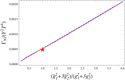
Figure 7: Right-handed neutrino production rate $\Gamma_{N}/(Y^{2}T^{4})$ for $g_{1,2}\to\tilde{g}_{1,2}$, $M_{N}=0$, varying $\tilde{g}_{1,2}$, and all remaining couplings as given in Table 1 for the scale $10^{9}{\rm GeV}$ (solid blue line). We also indicate the fit (100) (dashed red line) and indicate the rate in the SM (red star).

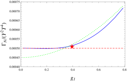
Figure 8: Right handed neutrino production rate $\Gamma_{N}/(Y^{2}T^{4})$ for $M_{N}=0$, varying $g_{1}$ and all remaining couplings as given in Table 1 for the scale $10^{9}\,{\rm GeV}$ (solid blue line). The dashed red line indicates the result for $g_{1}=0$, the dotted green line the fit (100). The rate in the SM is indicated by a red star.

The numerical results are presented in Figures 7 and 8. As in this work, we are interested in the production of light (relativistic) right-handed neutrinos and the scatterings of massless Standard Model leptons, gauge- and Higgs-bosons, we take for the mass $M_{N}$ of the right-handed neutrino $M_{N}=0$. For the Standard Model couplings implied by a Higgs boson mass of $125\,{\rm GeV}$, we thereby reproduce the value $\Gamma_{N}^{1\leftrightarrow 2}\approx 5\times 10^{-4}/(Y^{2}T^{4})$ found in Ref. [31]. Moreover, we find that a good fit to the behaviour apparent in Figure 7 is provided by

$$\Gamma_{N}^{1\leftrightarrow 2}/(Y^{2}T^{4})\approx 8.8\times 10^{-4}G\,.$$ (100)

The results presented in Figure 8 indicate that this formula becomes less accurate when one of the couplings is very small, i.e. we observe a deviation from the relation (100) when $g_{1}\ll g_{2}$.

Regarding the flavour equilibration rate $\gamma^{\rm fl}$, we note that the technique developed in Ref. [31] applies to diagrams of the type of Figure 5(C), where the gauge radiation originates from internal lines of the diagram in Figure 1 only, but not directly to the diagrams in Figures 5(A,B,D,E), where the gauge radiation also attaches to an external line. A generalisation of the methods developed in Ref. [31] is beyond the scope of the present work, but as we see below, the error from neglecting gauge radiation from an external line is quantitatively small compared to the dominating contribution from the $t$-channel exchange of fermions and the expected NLO corrections. In order to make an estimate for the relaxation rate of left-handed flavour $\gamma^{\rm fl}$, we notice that this should be complementary to the relaxation rate $\gamma_{R}^{\rm fl}$ for right-handed flavour,

$$\gamma^{\rm fl}=\frac{1}{2}\gamma_{R}^{\rm fl}\,,$$ (101)

where the factor $1/2$ is due to the multiplicity of left-handed leptons and Higgs bosons. Now, the right handed leptons ${\rm R}$ are different from the right-handed singlet neutrinos $N$ in that they have the weak hypercharge $-1$ and that within their self-energy diagram, no charge-conjugated particles are running. We may therefore approximate

$${\rm tr}[\not{p}\Sigma_{R}^{1\leftrightarrow 2}(p)]\approx\frac{1}{2}{\rm tr}[\not{p}\Sigma_{N}^{1\leftrightarrow 2}(p)]\,,$$ (102)

and from Figures 7 and 8, we can estimate the relative uncertainty due to inaccurately neglecting the ${\rm U}(1)$ weak hypercharge interactions by 15%. As it turns out that the $1\leftrightarrow 2$ rates are small compared to the sum of the $2\leftrightarrow 2$ rates (which are in turn dominated by the $t$-channel fermion exchange), and in view of the uncertainty from neglecting contributions $\propto G^{2}\log G^{-1}$ at the following order (NLO), it is therefore quantitatively sufficient to make the estimate

$${\rm tr}[\not{p}\Sigma_{\ell}^{1\leftrightarrow 2}(p)]\approx\frac{1}{4}{\rm tr}[\not{p}\Sigma_{N}^{1\leftrightarrow 2}(p)]\,.$$ (103)

Substitution into Eqs. (21) and (25) and numerical evaluation then yields (for the values of the couplings given in Table 1 at the scale of $10^{9}{\rm GeV}$)

$$\gamma^{\rm fl}_{1\leftrightarrow 2}=9.9\times 10^{-4}T\,.$$ (104)

When expressed as a fit similar to relation (100), this becomes

$$\gamma^{\rm fl}_{1\leftrightarrow 2}=1.7\times 10^{-3}GT\,.$$ (105)

6 Phenomenological Implications

6.1 Flavoured Leptogenesis

The full LO flavour equilibration rate has been calculated here for the first time. Adding the individual contributions, it can be expressed as

$$\gamma^{\rm fl} =\gamma^{{\rm fl}(\phi)\delta\ell}+\gamma^{{\rm fl}(\ell)\delta\ell}+\gamma^{{\rm fl}({\rm R})\delta\ell}+\gamma^{{\rm fl}}_{{\rm vertex}}$$ (106)

$$=1.32\times 10^{-3}\times h_{t}^{2}T+3.72\times 10^{-3}\times GT+8.31\times 10^{-4}\times G(\log G^{-1})T$$

$$+4.74\times 10^{-3}\times g_{1}^{2}T+1.67\times 10^{-3}\times g_{1}^{2}(\log g_{1}^{-2})T+1.7\times 10^{-3}GT\,,$$

where $G=\frac{1}{2}(3g_{2}^{2}+g_{1}^{2})$. From Section 3.3 we have used the numerical fit (64) since it is better behaved for small values of $p^{0}$.

The running of the couplings let $\gamma^{\rm fl}$ depend non-trivially on the temperature. In Figure 9 we show the individual contributions as well as the total flavour equilibration rate as function of the temperature, in the region of $T=10^{7}$ GeV to $10^{13}$ GeV. Note that the tree-level $1\to 2$ rate is zero in this temperature regime, since the thermal masses for the Higgs and for the leptons leave no phase space for a decay process. Only once the collinear emission contributions are included a finite $\gamma^{\rm fl}_{1\leftrightarrow 2}$ is obtained.

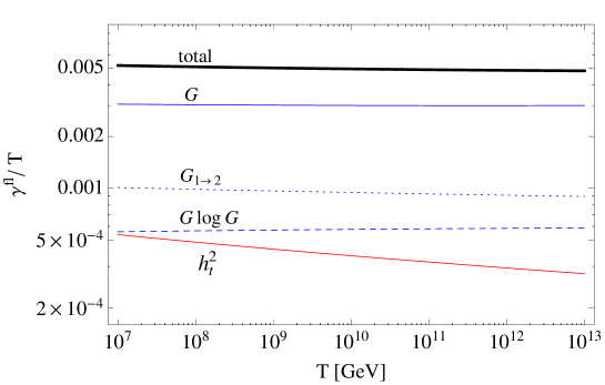
Figure 9: Individual contributions and total flavour equilibration rate $\gamma^{\rm fl}/T$ as function of the temperature $T$. The temperature dependence emerges through the renormalisation group equation (RGE) evolution of the coupling constants which are renormalised at the scale $2\pi T$. Earlier times appear to the right (higher temperature) in this plot. Contributions from gauge interactions are separated into linear and log enhanced scatterings as well as $1\to 2$ processes. The $g_{1}^{2}$ and $g_{1}^{2}(\log g_{1}^{-2})$ terms are included in the corresponding solid and dotted blue lines and in the total rate.

We see that the rate is largely dominated by the terms linear in $G$, which in turn receive their dominant contribution from the $t$-channel fermion exchange, as it is shown in detail in Section 3.3. The total rate varies between $5.19\times 10^{-3}T$ and $4.83\times 10^{-3}T$ (depending on the renormalisation scale). This is close to some estimates that were previously used in the literature, namely $5\times 10^{-3}T$ in [29, 44], but smaller than the value of $1.75\times 10^{-2}T$ used in [11]. In the light of the uncertainties due to the unknown NLO corrections, the improvement over the popular estimate of the flavour relaxation rate as $5\times 10^{-3}T$ may not be dramatic. We emphasise however that in contrast to the latter number, the relaxation rate obtained here derives from a systematic LO calculation. The estimates in Refs. [29, 44] go back to the work [46], where the $t$-channel divergences from fermion exchange are apparently regulated using the thermal fermion masses, but without including their widths, such that the numerical agreement is perhaps coincidental. Unfortunately, the estimation of the size of the NLO correction is not straightforward, such that presently, we cannot state a reliable number for the theoretical uncertainty, cf. the recently performed NLO calculation of the photon production rate in the quark-gluon plasma [43]. If we were taking the discrepancy between the semi-analytical expression (62) for the $t$-channel scattering rate and the numerical fit (64) as an indication of the theoretical uncertainty, we would estimate it as 15%.

When rescaling the results of Ref. [11] using the present LO value for the rate of flavour relaxation, we may conclude that the unflavoured description of Leptogenesis applies to masses for the decaying right-handed neutrino $M_{N}\gtrsim 10^{12}\,{\rm GeV}$, whereas it may be treated as fully flavoured (no correlations between the $\tau$-lepton doublets and the remaining two doublets) below masses of $M_{N}\;\raisebox{-3.00003pt}{$\stackrel{{\scriptstyle\displaystyle<}}{{\sim}}$}\;10^{11}\,{\rm GeV}$. This latter value lies below the sometimes estimated mass [45] of $M_{N}\;\raisebox{-3.00003pt}{$\stackrel{{\scriptstyle\displaystyle<}}{{\sim}}$}\;10^{12}\,{\rm GeV}$, where a flavoured description is assumed to be valid. Note that these are estimates obtained for two particular points in parameter space in Ref. [11], and we do not quote a quantitative error when applying either the unflavoured or flavoured description for a mass of the decaying right handed neutrino between $10^{11}\,{\rm GeV}$ and $10^{12}\,{\rm GeV}$. A more systematic and quantitative study of the transition between the flavoured and unflavoured regimes will be performed in the future.

The strong dependence on the gauge coupling strength also implies some model dependence of the flavour equilibration rate. In many extensions of the SM, the running of the gauge couplings is modified, such that the charged lepton Yukawa interactions will equilibrate at different temperature scales. A detailed phenomenological study of such variants of flavoured Leptogenesis will be presented elsewhere.

6.2 Results for the Right-Handed Neutrino Production Rate

The integrated rate for the production of right-handed singlet neutrinos can be obtained from the results of Sections 3 and 4 by performing the $p^{0}$ integration with a different weight, as explained in Section 2.5. The main purpose of performing this integration is to illustrate the size of the corrections compared with the tree-level calculation, and to facilitate comparison with the results of Ref. [32]. For a precise numerical study of Leptogenesis, one should instead use the differential distribution function $f_{N}(|\mathbf{p}|)$, since different momentum modes are equilibrated on different time scales, which can lead to a modification of the resulting lepton asymmetry [19].

The contributions to the neutrino production rate from Higgs and fermion mediated scatterings, from vertex-type diagrams and from collinearly enhanced $1\leftrightarrow 2$ processes are respectively given by

$$\gamma^{N(\phi)} =3.15\times 10^{-4}\times GT^{4}+5.22\times 10^{-4}\times h_{t}^{2}T^{4}\,,$$ (107)

$$\gamma^{N(\ell)} =2.24\times 10^{-3}\times GT^{4}+4.14\times 10^{-4}\times G(\log G^{-1})T^{4}\,,$$ (108)

$$\gamma^{N}_{\rm vert} =3.15\times 10^{-4}\times GT^{4}\,,$$ (109)

$$\gamma^{N}_{\rm 1\to 2} =8.8\times 10^{-4}\times GT^{4}\,,$$ (110)

where as before, $G=\frac{3}{2}g_{2}^{2}+\frac{1}{2}g_{1}^{2}$. The rate for $\gamma^{N(\ell)}$ is calculated using the analytical decomposition into linear and logarithmic contribution analogous to the procedure explained in Section 3.3. If instead one extracts the coefficients from a direct integration of (48) and by performing a numerical fit, one obtains

$$\gamma^{N(\ell)} =1.57\times 10^{-3}\times GT^{4}+3.67\times 10^{-4}\times G\log G^{-1}T^{4}\,.$$ (111)

See the end of Section 3.3 for a detailed discussion of how these two methods and results compare. Our numerical results should also be compared with those obtained in Ref. [32]. While we agree with the coefficient of the terms proportional to the top quark Yukawa and of the logarithmic term, we obtain a significantly larger coefficient for the term linear in $G$. Summing the terms linear in $G$ from the contributions (107)-(109), we obtain $2.87\times 10^{-3}\times GT^{4}$ compared to $1.00\times 10^{-3}\times GT^{4}$ in Ref. [32]. Using the resummed result for $\gamma^{N(\ell)}$ instead the linear coefficient is $2.20\times 10^{-3}\times GT^{4}$, still deviating significantly from Ref. [32]. In summary, our result for the production rate of right-handed neutrinos is

$$\gamma^{N}=3.08\times 10^{-3}\times GT^{4}+3.67\times 10^{-4}\times G\log G^{-1}T^{4}+5.22\times 10^{-4}\times h_{t}^{2}T^{4}\,.$$ (112)

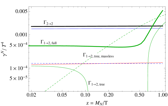
Figure 10: Individual contributions and total $N$ production rate $\gamma^{N}/T^{4}$, for zero $N$ density, as function of $z=M_{N}/T$ and $M_{N}=10^{11}$ GeV. The horizontal lines show the individual and total contributions from $2\to 2$ scattering processes. The green solid (dashed) lines show the tree level rate for $1\to 2$ processes with (without) thermal masses for the Higgs and lepton doublet, while the thick green line shows the $1\to 2$ rate including the collinear enhancements. Note that as before, the $2\to 2$ scattering rates are calculated in the $M_{N}=0$ approximation and therefore only valid for $z\lesssim 1$. Different from Figure 9, time flows from left to right here as the Universe is cooling.

In Figure 10, we show the different contributions to $N$ production for vanishing density of $N$, $f_{N}(p)=0$. We see that while the collinear enhancement of $N$ production is significant when compared to the tree level rates, the gauge mediated scatterings dominate at high temperatures ($z\ll 1$), while the tree level $\phi\to N\ell$ decay plays a negligible role for $N$ production. Before $z>1$, the $M_{N}=0$ approximation used for calculating the scattering rates becomes invalid. Results for the ${\cal O}(g^{2})$ corrections for $N$ production in this non-relativistic regime were recently reported in Refs. [38, 39].

Since the tree level rates are small compared to the scattering contributions in the high temperature regime, a precise calculation of the lepton asymmetry in this regime not only needs to take scatterings into account for the washout effects, but also should include them in the calculation of the $CP$ asymmetry. This is particularly important for Leptogenesis in the weak washout regime and should therefore be addressed in the future.

7 Conclusions

In this work, we have presented an approach based on the CTP formalism to calculate interaction rates at finite temperature from 2PI self energies. This we have employed to calculate the flavour relaxation and the right-handed neutrino production rates relevant for Leptogenesis scenarios. The main results of the present paper are:

• We have shown that finite temperature interaction rates can be calculated perturbatively in the 2PI formalism. Using this approach, the $t$-channel divergences in diagrams with fermion exchange are automatically regulated. The linear and logarithmic dependencies on the gauge-coupling square introduced by such processes can be extracted both analytically and by a numerical fit from our calculation.

• The LO results for the flavour relaxation rates and right-handed neutrino production rates and their dependence on the gauge and top Yukawa couplings are given in Section 6. These expressions can easily be used for obtaining interaction rates in other models, since the dependencies on the temperature, gauge-coupling evolution and hypercharge assignment are given explicitly.

• We find that both rates are largely dominated by the fermion-mediated $t$-channel scatterings, and are therefore sensitive to the RGE evolution of the gauge couplings. The coefficients vary by about 15% depending on whether they are extracted analytically or numerically. Since the numerical fit (64) includes an incomplete account of higher order effects through resummation, this deviation can be taken as an indication for the magnitude of higher order effects.

• While a detailed study of the impact on flavour effects remains to be done, we can already conjecture in combination with the work [11] that the unflavoured description of Leptogenesis will be valid for $M_{N}$ as low as $5\times 10^{11}$ GeV, somewhat lower than previously estimated.

The production rate of right-handed singlet neutrinos for vanishing $N$ density was previously calculated in Ref. [32]. While we agree with the coefficients of the $G\log G$ and $h_{t}^{2}$ terms, we find a much larger coefficient for the contributions linear in $G$ which dominates the overall $N$ production rate. This also reduces the absolute importance of the collinear scatterings that were first shown to be relevant in [31]. Further investigations are required to identify the origin of this discrepancy. To this end, we note that our semi-analytical extraction of the terms linear and logarithmic in $G$ agrees within the expected accuracy with a numerical evaluation of the phase-space integrals, which can be taken as a consistency check.

Our calculations have been performed in the approximation that all masses of the external particles are vanishingly small. This is a good approximation for the flavour relaxation rate, where all particles have masses ${\cal O}(gT)$ that only lead to small, NLO, corrections since interactions in the plasma are dominated by hard processes with ${\cal O}(T)$ momentum exchange. For the right-handed neutrino production rate, this approximation breaks down when $M_{N}\gtrsim T$, i.e. at times where $z>1$. In this regime $1\to 3$ decays of $N$ are kinematically allowed and exhibit divergences when the emitted gauge boson is soft or collinear with one of the other decay products. These divergences should be cancelled by virtual corrections that arise when only two propagators are put on shell in the diagrams in Figure  5. For the $T\ll M_{N}$ limit, this cancellation was recently demonstrated in [38, 39]. Using the approach presented here, it has been shown that the cancellation of soft and collinear divergences occurs for any temperature [40].

Extensions and applications of the calculation of LO scattering and production rates for light (compared to the temperature) particles include a calculation of the $CP$-violating rate in the weak washout regime of Leptogenesis. Besides, a systematic and quantitative study of the transition regime between flavoured and unflavoured Leptogenesis may now be performed in combination with the description of flavour decoherence developed in Ref. [11]. The results of this work may therefore serve as a basis for LO calculations of the baryon asymmetry of the Universe in scenarios where so far, only estimates have been available.

Appendix A RGE evolution of couplings

The gauge and top quark Yukawa couplings at temperature scales relevant for Leptogenesis differ significantly from their values at the Electroweak scale. The RGE evolution is well known in the SM. At the one-loop level, the gauge couplings at a scale $\mu$ are given by

$$\alpha_{i}^{-1}(\mu)=\alpha_{i}^{-1}(M_{Z})-\frac{b_{i}}{2\pi}\log\left(\frac{\mu}{M_{Z}}\right),$$ (113)

where $b_{1}=41/10$, $b_{2}=-19/6$ and $b_{3}=-7$, and the $\alpha_{i}(M_{Z})$ are the values of the couplings at the Electroweak scale. The couplings $\alpha_{i}$ are defined as $\alpha_{1}=\frac{5}{3}g_{1}^{2}/(4\pi)$ and $\alpha_{2,3}=g^{2}_{2,3}/(4\pi)$, following the conventions used in the context of Grand Unification.

The RGE equations for the top Yukawa and the Higgs quartic coupling at the one loop level are given by [47]

$$\mu\frac{d}{d\mu}h_{t}^{2} =\frac{9}{2}\frac{1}{8\pi^{2}}h_{t}^{2}\left(h_{t}^{2}-4\pi\left(\frac{17}{54}\alpha_{1}+\frac{1}{2}\alpha_{2}+\frac{16}{9}\alpha_{3}\right)\right),$$ (114)

$$\mu\frac{d}{d\mu}\lambda =\frac{6}{8\pi^{2}}\left(\lambda^{2}-4\pi\lambda\left(\frac{\alpha_{1}}{4}+\frac{3}{4}\alpha_{2}-\frac{h_{t}^{2}}{4\pi}\right)+(4\pi)^{2}\left(\frac{\alpha_{1}^{2}}{16}+\frac{\alpha_{1}\alpha_{2}}{8}+\frac{3}{16}\alpha_{2}^{2}\right)-h_{t}^{4}\right),$$ (115)

where we suppress the dependence of the couplings on the RGE scale $\mu$. These are evaluated numerically using the following input values for the gauge and top Yukawa couplings at the Electroweak scale [48]: $\alpha_{1}(M_{Z})=0.0169$, $\alpha_{2}(M_{Z})=0.0338$, $\alpha_{3}(M_{Z})=0.1184$ and $h_{t}(M_{Z})=0.998$.

The Higgs quartic coupling depends on the Higgs boson mass through $\lambda=(m_{h}/v)^{2}/2$, where $v=174$ GeV. Current experimental constraints indicate that $m_{h}=125$ GeV, which we take as the value of the Higgs boson mass for the rest of this analysis.

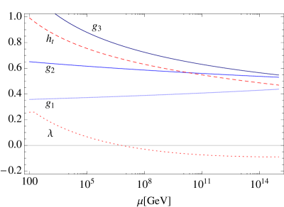
Figure 11: One-loop evolution of coupling constants in the SM. Note that $g_{1}=\sqrt{3/5}\,g_{1,{\rm GUT}}$, such that gauge coupling unification at $\mu\sim 10^{15}$ GeV is not evident in this figure.

The evolution of the couplings up to scales $\mu=10^{15}$ GeV is shown in Figure 11. The value of the Higgs quartic coupling gets negative at intermediate scales, which could jeopardise the stability of the Electroweak vacuum. A more detailed study, including two loop corrections and threshold effects, was presented in [49]. They find that while the Higgs coupling indeed becomes negative at high scales, it stays above the meta-stability bound for $m_{h}\sim 125$ GeV, and the upper limit on the reheating temperature is consistent with the Leptogenesis scenario.

RGE scale	$g_{1}$	$g_{2}$	$g_{3}$	$h_{t}$	$\lambda$
$10^{9}$ GeV	0.394	0.577	0.689	0.600	-0.049
$10^{12}$ GeV	0.414	0.552	0.606	0.526	-0.082

Table 1: Values of the relevant SM coupling constants at scales important for Leptogenesis.

The values of the couplings for $\mu=10^{9}$ GeV and $\mu=10^{12}$ GeV are given in Table 1. These values are used for the numerical analysis in Section 6.1. The running of the couplings in the relevant temperature regime is relatively slow, such that it is not necessary to evolve the couplings along with the temperature in a numerical analysis. The induced uncertainty is of higher order in the coupling expansion.

Appendix B Feynman Rules

For completeness, here we list the Feynman rules that are employed to calculate the one and two-loop self energies directly in Wigner space. First, note that the standard definition, in Wigner space, is such that

where the blob denotes the sum of all one particle irreducible (1PI) diagrams, the momentum flows in the direction of the arrows, and the external legs are understood to be amputated.

For fermions (and similarly for complex scalars), the two-point correlation-functions on the closed time path (CTP) are defined as

$${\rm i}S(u,v) =\left\langle T_{\cal C}(\psi(u)\bar{\psi}(v))\right\rangle,$$ (116)

where $T_{\cal C}$ denotes time ordering along the CTP. Since $\bar{\psi}$ creates a fermion state and annihilates an anti-fermion, an arrow indicating particle flow will point from $v$ to $u$. Correspondingly, we obtain the following Feynman rules for the propagators in momentum space:

$$={\rm i}\Delta^{ab}(k)\,,$$ (117)

$$={\rm i}S^{ab}(k)\,.$$ (118)

Our convention that the SU(2) doublets are defined as $\phi=(\phi^{+},\phi^{0})^{T}$ and $\ell_{i}=(\nu_{i},e_{i}^{-})^{T}$ implies that the arrows point in the direction of positive (negative) electric charge flow for Higgs bosons (SM leptons). The momentum flows in the direction of the arrow. Since the gauge boson propagators are neutral, the propagators have no well defined charge flow. Note that we suppress all $SU(2)$ indices in this paper.

Interactions

- Interaction vertices are derived from the Lagrangian as in conventional field theory. In addition, each internal vertex obtains a sign $a\in\{+,-\}$ that is summed over. The following vertices are relevant for the calculations in this paper:

$\qquad-{\rm i}hP_{\rm L}\,,$

$\qquad-{\rm i}h^{\dagger}P_{\rm R}\,,$

where we have suppressed gauge and flavour indices. For gauge boson interactions we make the gauge indices explicit:

$$-{\rm i}g_{1}\gamma^{\mu}(Y_{\rm L}P_{\rm L}+Y_{\rm R}P_{\rm R})\delta_{fg}\quad \text{for }V^{A}=B\,,$$

$$-{\rm i}g_{2}\gamma^{\mu}P_{\rm L}T^{A}_{fg} \text{for }V^{A}=W^{A}\,,$$

$$-{\rm i}g_{1}Y_{\phi}\delta_{fg}\left(p+k\right)^{\mu}\quad \text{for }V^{A}=B\,,$$

$$-{\rm i}g_{2}T^{A}_{fg}\left(p+k\right)^{\mu} \text{for }V^{A}=W^{A}\,.$$

Here $T^{A}_{fg}$ are the generators of SU(2) in the fundamental representation, $p,k,q$ denote the momenta and $f,g$ are SU(2) indices. The scalar-scalar-vector (SSV) vertex is particularly sensitive to sign errors. The rule presented above is valid provided that both the momenta and the positive charge flows in the direction indicated by the arrows.

References

• [1] M. Fukugita and T. Yanagida, “Baryogenesis Without Grand Unification,” Phys. Lett. B 174 (1986) 45.
• [2] W. Buchmuller, “Leptogenesis: Theory and Neutrino Masses,” arXiv:1210.7758 [hep-ph].
• [3] S. Blanchet and P. Di Bari, “The minimal scenario of leptogenesis,” New J. Phys.  14 (2012) 125012 [arXiv:1211.0512 [hep-ph]].
• [4] C. S. Fong, E. Nardi and A. Riotto, “Leptogenesis in the universe,” Adv. High Energy Phys.  2012 (2012) 158303 [arXiv:1301.3062 [hep-ph]].
• [5] J. S. Schwinger, “Brownian motion of a quantum oscillator,” J. Math. Phys.  2 (1961) 407.
• [6] L. V. Keldysh, “Diagram technique for nonequilibrium processes,” Zh. Eksp. Teor. Fiz.  47 (1964) 1515 [Sov. Phys. JETP 20 (1965) 1018].
• [7] E. Calzetta and B. L. Hu, “Nonequilibrium Quantum Fields: Closed Time Path Effective Action, Wigner Function and Boltzmann Equation,” Phys. Rev.  D 37 (1988) 2878.
• [8] W. Buchmuller and S. Fredenhagen, “Quantum mechanics of baryogenesis,” Phys. Lett. B 483, 217 (2000) [hep-ph/0004145].
• [9] A. De Simone and A. Riotto, “Quantum Boltzmann Equations and Leptogenesis,” JCAP 0708 (2007) 002 [hep-ph/0703175].
• [10] V. Cirigliano, C. Lee, M. J. Ramsey-Musolf and S. Tulin, “Flavored Quantum Boltzmann Equations,” Phys. Rev. D 81 (2010) 103503 [arXiv:0912.3523 [hep-ph]].
• [11] M. Beneke, B. Garbrecht, C. Fidler, M. Herranen and P. Schwaller, “Flavoured Leptogenesis in the CTP Formalism,” Nucl. Phys. B 843 (2011) 177 [arXiv:1007.4783 [hep-ph]].
• [12] A. Anisimov, W. Buchmuller, M. Drewes and S. Mendizabal, “Quantum Leptogenesis I,” Annals Phys.  326 (2011) 1998 [arXiv:1012.5821 [hep-ph]].
• [13] L. Covi, N. Rius, E. Roulet and F. Vissani, “Finite temperature effects on CP violating asymmetries,” Phys. Rev. D 57 (1998) 93 [hep-ph/9704366].
• [14] G. F. Giudice, A. Notari, M. Raidal, A. Riotto and A. Strumia, “Towards a complete theory of thermal leptogenesis in the SM and MSSM,” Nucl. Phys. B 685 (2004) 89 [hep-ph/0310123].
• [15] M. Garny, A. Hohenegger, A. Kartavtsev and M. Lindner, “Systematic approach to leptogenesis in nonequilibrium QFT: vertex contribution to the CP-violating parameter,” Phys. Rev.  D 80 (2009) 125027 [arXiv:0909.1559 [hep-ph]].
• [16] M. Garny, A. Hohenegger, A. Kartavtsev and M. Lindner, “Systematic approach to leptogenesis in nonequilibrium QFT: self-energy contribution to the CP-violating parameter,” Phys. Rev.  D 81 (2010) 085027 [arXiv:0911.4122 [hep-ph]].
• [17] A. Anisimov, W. Buchmüller, M. Drewes and S. Mendizabal, “Leptogenesis from Quantum Interference in a Thermal Bath,” Phys. Rev. Lett.  104 (2010) 121102 [arXiv:1001.3856 [hep-ph]].
• [18] M. Garny, A. Hohenegger, A. Kartavtsev, “Medium corrections to the CP-violating parameter in leptogenesis,” Phys. Rev.  D81 (2010) 085028. [arXiv:1002.0331 [hep-ph]].
• [19] M. Beneke, B. Garbrecht, M. Herranen and P. Schwaller, “Finite Number Density Corrections to Leptogenesis,” Nucl. Phys. B 838 (2010) 1 [arXiv:1002.1326 [hep-ph]].
• [20] B. Garbrecht, “Leptogenesis: The Other Cuts,” Nucl. Phys.  B847 (2011) 350-366. [arXiv:1011.3122 [hep-ph]].
• [21] B. Garbrecht and M. Herranen, “Effective Theory of Resonant Leptogenesis in the Closed-Time-Path Approach,” Nucl. Phys. B 861 (2012), 17. [arXiv:1112.5954 [hep-ph]].
• [22] M. Garny, A. Kartavtsev and A. Hohenegger, “Leptogenesis from first principles in the resonant regime,” Annals Phys.  328 (2013) 26 [arXiv:1112.6428 [hep-ph]].
• [23] B. Garbrecht, “Leptogenesis from Additional Higgs Doublets,” Phys. Rev. D 85 (2012) 123509 [arXiv:1201.5126 [hep-ph]].
• [24] M. Drewes and B. Garbrecht, “Leptogenesis from a GeV Seesaw without Mass Degeneracy,” to appear in JHEP [arXiv:1206.5537 [hep-ph]].
• [25] B. Garbrecht, “Baryogenesis from Mixing of Lepton Doublets,” Nucl. Phys. B 868 (2013) 557 [arXiv:1210.0553 [hep-ph]].
• [26] T. Frossard, M. Garny, A. Hohenegger, A. Kartavtsev and D. Mitrouskas, “Systematic approach to thermal leptogenesis,” arXiv:1211.2140 [hep-ph].
• [27] P. Millington and A. Pilaftsis, “Perturbative Non-Equilibrium Thermal Field Theory,” arXiv:1211.3152 [hep-ph].
• [28] T. Endoh, T. Morozumi and Z. -h. Xiong, “Primordial lepton family asymmetries in seesaw model,” Prog. Theor. Phys.  111, 123 (2004) [hep-ph/0308276].
• [29] A. Abada, S. Davidson, F. -X. Josse-Michaux, M. Losada and A. Riotto, “Flavor issues in leptogenesis,” JCAP 0604, 004 (2006) [hep-ph/0601083].
• [30] E. Nardi, Y. Nir, E. Roulet and J. Racker, “The Importance of flavor in leptogenesis,” JHEP 0601, 164 (2006) [hep-ph/0601084].
• [31] A. Anisimov, D. Besak, D. Bodeker, “Thermal production of relativistic Majorana neutrinos: Strong enhancement by multiple soft scattering,” JCAP 1103 (2011) 042. [arXiv:1012.3784 [hep-ph]].
• [32] D. Besak and D. Bodeker, “Thermal production of ultrarelativistic right-handed neutrinos: Complete leading-order results,” JCAP 1203, 029 (2012) [arXiv:1202.1288 [hep-ph]].
• [33] C. P. Kiessig, M. Plumacher and M. H. Thoma, “Decay of a Yukawa fermion at finite temperature and applications to leptogenesis,” Phys. Rev. D 82 (2010) 036007 [arXiv:1003.3016 [hep-ph]].
• [34] C. Kiessig and M. Plumacher, “Hard-Thermal-Loop Corrections in Leptogenesis I: CP-Asymmetries,” JCAP 1207 (2012) 014 [arXiv:1111.1231 [hep-ph]].
• [35] C. Kiessig and M. Plumacher, “Hard-Thermal-Loop Corrections in Leptogenesis II: Solving the Boltzmann Equations,” JCAP 1209 (2012) 012 [arXiv:1111.1235 [hep-ph]].
• [36] P. B. Arnold, G. D. Moore and L. G. Yaffe, “Transport coefficients in high temperature gauge theories. 1. Leading log results,” JHEP 0011 (2000) 001 [hep-ph/0010177].
• [37] P. B. Arnold, G. D. Moore and L. G. Yaffe, “Photon emission from quark gluon plasma: Complete leading order results,” JHEP 0112 (2001) 009 [hep-ph/0111107].
• [38] A. Salvio, P. Lodone and A. Strumia, “Towards leptogenesis at NLO: the right-handed neutrino interaction rate,” JHEP 1108 (2011) 116 [arXiv:1106.2814 [hep-ph]].
• [39] M. Laine and Y. Schroder, “Thermal right-handed neutrino production rate in the non-relativistic regime,” JHEP 1202 (2012) 068 [arXiv:1112.1205 [hep-ph]].
• [40] B. Garbrecht, F. Glowna and M. Herranen, “Right-Handed Neutrino Production at Finite Temperature: Radiative Corrections, Soft and Collinear Divergences,” to appear in JHEP [arXiv:1302.0743 [hep-ph]].
• [41] T. Prokopec, M. G. Schmidt and S. Weinstock, “Transport equations for chiral fermions to order h bar and electroweak baryogenesis. Part 1,” Annals Phys.  314 (2004) 208 [hep-ph/0312110].
• [42] B. Garbrecht and T. Konstandin, “Separation of Equilibration Time-Scales in the Gradient Expansion,” Phys. Rev. D 79, 085003 (2009) [arXiv:0810.4016 [hep-ph]].
• [43] J. Ghiglieri, J. Hong, A. Kurkela, E. Lu, G. D. Moore and D. Teaney, “Next-to-leading order thermal photon production in a weakly coupled quark-gluon plasma,” arXiv:1302.5970 [hep-ph].
• [44] S. Blanchet and P. Di Bari, “Flavor effects on leptogenesis predictions,” JCAP 0703 (2007) 018 [hep-ph/0607330].
• [45] A. Abada, S. Davidson, A. Ibarra, F. -X. Josse-Michaux, M. Losada and A. Riotto, “Flavour Matters in Leptogenesis,” JHEP 0609 (2006) 010 [hep-ph/0605281].
• [46] J. M. Cline, K. Kainulainen and K. A. Olive, “Protecting the primordial baryon asymmetry from erasure by sphalerons,” Phys. Rev. D 49 (1994) 6394 [hep-ph/9401208].
• [47] M. Lindner, “Implications of Triviality for the Standard Model,” Z. Phys. C 31 (1986) 295.
• [48] K. Nakamura et al. [Particle Data Group Collaboration], “Review of particle physics,” J. Phys. G G 37 (2010) 075021.
• [49] J. Elias-Miro, J. R. Espinosa, G. F. Giudice, G. Isidori, A. Riotto and A. Strumia, “Higgs mass implications on the stability of the electroweak vacuum,” arXiv:1112.3022 [hep-ph].