Abstract

Manifold learning has been successfully applied to a variety of medical imaging problems. Its use in real-time applications requires fast projection onto the low-dimensional space. To this end, out-of-sample extensions are applied by constructing an interpolation function that maps from the input space to the low-dimensional manifold. Commonly used approaches such as the Nyström extension and kernel ridge regression require using all training points. We propose an interpolation function that only depends on a small subset of the input training data. Consequently, in the testing phase each new point only needs to be compared against a small number of input training data in order to project the point onto the low-dimensional space. We interpret our method as an out-of-sample extension that approximates kernel ridge regression. Our method involves solving a simple convex optimization problem and has the attractive property of guaranteeing an upper bound on the approximation error, which is crucial for medical applications. Tuning this error bound controls the sparsity of the resulting interpolation function. We illustrate our method in two clinical applications that require fast mapping of input images onto a low-dimensional space.

1 Introduction

Manifold learning maps high-dimensional data to a low-dimensional manifold and has recently been successfully applied to a variety of applications. Specifically in medical imaging, manifold learning has been used in segmentation [24], registration [12, 15], computational anatomy [11], classification [6, 22], detection [20], and respiratory gating [10, 23]. But to the best of our knowledge, little work has been done using manifold learning for medical imaging applications that require fast projections onto a low-dimensional space.

In this paper, we demonstrate a method that achieves fast projection of input data onto a low-dimensional manifold by constructing a projection function that only depends on a small subset of the training data. Our method is a sparse variant of kernel ridge regression [18] and can be interpreted as an interpolation function optimized to only use a few of the training data. Furthermore, the construction of the interpolation function guarantees an upper bound on an interpolation error for training data. The error is measured in terms of the average squared Euclidean distance between the predicted points of the interpolator versus those of kernel ridge regression using all the points. As our interpolator has no parametric model for the data points, its complexity is driven by the complexity of the training data and the bound on the approximation error.

Related work on out-of-sample extensions. Manifold learning is a specific case of nonlinear dimensionality reduction and refers to a host of different algorithms [13]. In medical image analysis, manifold learning is used to construct a low-dimensional space for images in which subsequent statistical analysis (regression, classification, etc.) is performed. Many manifold learning techniques do not construct a mapping of the entire input space but only of the training points. For these methods, estimating a new point’s location in the low-dimensional space is performed via an out-of-sample extension [5], with Nyström extensions commonly used. For certain manifold learning methods, a Nyström extension is a special case of kernel ridge regression [19], and for both the Nyström extension and kernel ridge regression, the resulting interpolation function for mapping a new input point to the low-dimensional space depends on all training data. Thus, we need to compare a new point to all training data points, which is computationally expensive for volumetric images, especially if the number of input data used to learn the manifold is large.

Our work is most similar to reduced rank kernel ridge regression [7], which also approximates kernel ridge regression by only using a small number of input training points. Reduced rank kernel ridge regression greedily selects training points to minimize a particular cost function. Specifically, the algorithm incrementally adds a training point that causes the largest decrease in overall cost. Different criteria could be used for when the greedy procedure is terminated such as if a pre-specified desired number of training points to use is reached or if the overall cost drops below a pre-specified desired error tolerance. Importantly, for medical applications, the latter criterion is more directly connected to the error analysis of the whole processing pipeline. Our approach also requires the user to specify a desired error tolerance but uses a different cost function. Rather than using a greedy approach to select which training points to add, we solve a convex optimization problem implied by our cost function. We remark that the proposed cost function also differs from that of support vector regression [9], which essentially achieves sparsity via excluding training points that map sufficiently close to the estimated function. Our cost is more lenient, asking that an average error be small rather than asking that an error be small for each individual training point.

Contributions. For high-dimensional input points $x_{1},x_{2},\dots,x_{n}\in\mathbb{R}^{d}$ and their low-dimensional representations $y_{1},y_{2},\dots,y_{n}\in\mathbb{R}^{p}$ as computed by any manifold learning algorithm, we propose a convex program for constructing an out-of-sample extension that guarantees a bound on the approximation error. Formally, if $\widehat{f}:\mathbb{R}^{d}\rightarrow\mathbb{R}^{p}$ is the out-of-sample extension function estimated via kernel ridge regression, then the sparse projection function $\widetilde{f}:\mathbb{R}^{d}\rightarrow\mathbb{R}^{p}$ constructed by our algorithm satisfies

$$\frac{1}{n}\sum_{i=1}^{n}\|\widehat{f}(x_{i})-\widetilde{f}(x_{i})\|_{2}^{2}\leq\varepsilon^{2},$$ (1)

where $\|\cdot\|_{2}$ denotes the Euclidean norm, $\varepsilon>0$ is a pre-specified error tolerance, and $\widetilde{f}$ depends only on a small subset of $x_{1},\dots,x_{n}$. The size of the subset, i.e., the sparsity of the resulting function $\widetilde{f}$, depends on tolerance $\varepsilon$ and training pairs $(x_{1},y_{1}),\dots,(x_{n},y_{n})$. Finding the smallest such subset is NP-hard. We instead consider a convex relaxation with sparsity induced by a mixed $\ell_{1}/\ell_{2}$ norm. While the proposed sparse approximation to kernel ridge regression can be used more generally for other multivariate regression tasks, we restrict our focus in this paper to out-of-sample extensions for manifold learning.

We apply our method to two medical imaging applications that require a fast projection onto a low-dimensional space. The first application is respiratory gating in ultrasound, where we assign the breathing state to each ultrasound frame during the acquisition in real-time. The second application is the estimation of a patient’s position in a magnetic resonance imaging (MRI) scanner while the patient is being moved to a target location.

2 Background

Our method builds heavily on kernel ridge regression [18], reviewed below. We also briefly discuss the result that a Nyström extension is a special case of kernel ridge regression under certain conditions [19]. As a consequence, our sparse approximation to kernel ridge regression also contains a sparse approximation to the widely used Nyström extension.

Kernel ridge regression. Let $\mathbb{H}$ be a family of functions mapping $\mathbb{R}^{d}$ to $\mathbb{R}$ such that $\mathbb{H}$ is a reproducing kernel Hilbert space (RKHS) [1] with kernel function $\mathbb{K}:\mathbb{R}^{d}\times\mathbb{R}^{d}\rightarrow\mathbb{R}$. Given points $x_{1},\dots,x_{n}\in\mathbb{R}^{d}$ and ${y_{1},\dots,y_{n}\in\mathbb{R}^{p}}$, we assume that there exists a function $f^{*}=(f^{*}_{1},\dots,f^{*}_{p})\in\mathbb{H}^{p}$ such that for each $i$, we have $y_{i}=f^{*}(x_{i})+w_{i}$ for some noise term $w_{i}\in\mathbb{R}^{p}$. Kernel ridge regression seeks an estimate $\widehat{f}$ of function $f^{*}$ by solving

$$\widehat{f}=\underset{(f_{1},\dots,f_{p})\in\mathbb{H}^{p}}{\text{argmin}}\sum_{j=1}^{p}\left\{\sum_{i=1}^{n}(Y_{ij}-f_{j}(x_{i}))^{2}+\lambda\|f_{j}\|_{\mathbb{H}}^{2}\right\},$$ (2)

where matrix $Y\in\mathbb{R}^{n\times p}$ contains data point $y_{i}$ as its $i$-th row, constant $\lambda>0$ controls the amount of regularization, and $\|\cdot\|_{\mathbb{H}}$ is the norm induced by the inner product of $\mathbb{H}$. The solution of optimization problem (2) is

$$\widehat{f}(\cdot)=\sum_{i=1}^{n}\mathbb{K}(\cdot,x_{i})\widehat{\alpha}_{i},$$ (3)

where $\widehat{\alpha}_{i}$ refers to the $i$-th row of $n$-by-$p$ matrix

$$\widehat{\alpha}=\left(K+\lambda I_{n\times n}\right)^{-1}Y,$$ (4)

matrix $K\in\mathbb{R}^{n\times n}$ is given by $K_{ij}=\mathbb{K}(x_{i},x_{j})$, and $I_{n\times n}$ is the $n\text{-by-}n$ identity matrix [18].

Nyström extension. The Nyström method approximates a certain type of eigenfunction problem and is used for out-of-sample extensions in manifold learning [5]. For manifold learning algorithms that assign the low-dimensional coordinates directly from the eigenvectors of $K$, e.g., Isomap [21], locally linear embeddings [17], and Laplacian eigenmaps [4], we can derive the Nyström extension as a special case of kernel ridge regression with $\lambda=0$. Specifically, with eigendecomposition $K=\Phi\Lambda\Phi^{-1}$, where $\Lambda=\text{diag}(\lambda_{1},\lambda_{2},\dots,\lambda_{n})$ and $\lambda_{1}\geq\lambda_{2}\geq\cdots\geq\lambda_{n}$, we consider when the low-dimensional embedding is given by $Y=\Phi_{\ell}$, the matrix consisting of the first $\ell$ columns of $\Phi$. If we use $\phi^{(j)}$ to denote the $j$-th column of $\Phi$, then with $\lambda=0$ and $Y=\Phi_{\ell}$, eq. (4) reduces to

$$\widehat{\alpha}=K^{-1}Y=\Phi\Lambda^{-1}\Phi^{-1}\Phi_{\ell}=\Phi\Lambda^{-1}\begin{bmatrix}I_{\ell\times\ell}\\ \mathbf{0}\end{bmatrix}=\begin{bmatrix}\frac{1}{\lambda_{1}}\phi^{(1)}\rotatebox[origin={c}]{90.0}{$\dabar@\dabar@\dabar@$}&\frac{1}{\lambda_{2}}\phi^{(2)}\rotatebox[origin={c}]{90.0}{$\dabar@\dabar@\dabar@$}&\cdots\rotatebox[origin={c}]{90.0}{$\dabar@\dabar@\dabar@$}&\frac{1}{\lambda_{\ell}}\phi^{(\ell)}\end{bmatrix}.$$ (5)

Letting $\phi_{i}^{(j)}$ refer to the $i$-th element of $\phi^{(j)}$, and substituting eq. (5) into eq. (3), we see that, for a new point $x\in\mathbb{R}^{d}$, the $j$-th element of $\widehat{f}(x)$ is given by

$$\widehat{f}_{j}(x)=\sum_{i=1}^{n}\mathbb{K}(x,x_{i})\widehat{\alpha}_{ij}=\sum_{i=1}^{n}\mathbb{K}(x,x_{i})\left(\frac{1}{\lambda_{j}}\phi_{i}^{(j)}\right)=\frac{1}{\lambda_{j}}\sum_{i=1}^{n}\phi_{i}^{(j)}\mathbb{K}(x,x_{i}),$$ (6)

which is the formula for the low-dimensional embedding of $x$ using the Nyström extension [5]. Importantly, kernel function $\mathbb{K}$ depends on the choice of a manifold learning algorithm [5]. The above relationship shows that for certain manifold learning algorithms, kernel ridge regression is a richer model for out-of-sample extensions than the Nyström extension.

3 Sparse Approximation to Kernel Ridge Regression

We now present our method. We seek an interpolation function $\widetilde{f}:\mathbb{R}^{d}\rightarrow\mathbb{R}^{p}$ within a family of functions $\mathbb{G}=\{f(\cdot)=\sum_{i=1}^{n}\mathbb{K}(\cdot,x_{i})\alpha_{i}:\alpha\in\mathbb{R}^{n\times p}\}$, with many vectors $\alpha_{i}\in\mathbb{R}^{p}$ equal to zero while ensuring that upper bound (1) holds. In particular, we formulate a convex optimization problem where $\alpha\in\mathbb{R}^{n\times p}$ is the only decision variable; solving this problem yields $\widetilde{\alpha}$ that implies a sparse approximation $\widetilde{f}$ to the kernel ridge regression solution $\widehat{f}$.

Because we optimize over functions in $\mathbb{G}$, upper bound (1) can be simplified by noting that ${\sum_{i=1}^{n}\|\widehat{f}(x_{i})-f(x_{i})\|_{2}^{2}}={\|K\widehat{\alpha}-K\alpha\|_{F}^{2}}$, where $\|\cdot\|_{F}$ denotes the Frobenius norm, and $\widehat{\alpha}$ is given by eq. (4). In fact, $\widehat{f}(x_{i})$ and $f(x_{i})$ are given by the $i$-th rows of $K\widehat{\alpha}$ and $K\alpha$, respectively. Thus, bound (1) can be rewritten as $\|K\widehat{\alpha}-K\alpha\|_{F}^{2}\leq n\varepsilon^{2}$. Satisfying this constraint while encouraging the number of nonzero vectors $\alpha_{i}$ to be small can be achieved by solving the following convex optimization problem:

$$\widetilde{\alpha}=\underset{\alpha\in\mathbb{R}^{n\times p}}{\text{argmin}}\sum_{i=1}^{n}\|\alpha_{i}\|_{2}\qquad\text{s.t.}\qquad\|K\widehat{\alpha}-K\alpha\|_{F}^{2}\leq n\varepsilon^{2}.$$ (7)

By minimizing the mixed $\ell_{1}/\ell_{2}$ norm of $\alpha$, we encourage each vector $\alpha_{i}$ to either consist of all zeros or all non-zero entries [2]. Note that if $p=1$ and we instead ask for the sparsest solution possible, then the objective function becomes the $\ell_{0}$ norm (i.e., the number of nonzero elements) of $\alpha$, and the optimization problem itself becomes NP-hard [14].

To solve optimization problem (7), we reduce it to solving many instances of its unconstrained Lagrangian form for which there is already a fast solver. Specifically, by Lagrangian duality and convexity, solving optimization problem (7) is equivalent to solving the dual problem

$$\max_{\xi\geq 0}\min_{\alpha\in\mathbb{R}^{n\times p}}\left\{\sum_{i=1}^{n}\|\alpha_{i}\|_{2}+\xi\big{(}\|K\widehat{\alpha}-K\alpha\|_{F}^{2}-n\varepsilon^{2}\big{)}\right\}\\ =\sup_{\xi>0}\xi\big{[}g(1/\xi)-n\varepsilon^{2}\big{]},$$ (8)

where $\xi$ is a Lagrange multiplier, and

$$g(\gamma)=\min_{\alpha\in\mathbb{R}^{n\times p}}\left\{\|K\widehat{\alpha}-K\alpha\|_{F}^{2}+\gamma\sum_{i=1}^{n}\|\alpha_{i}\|_{2}\right\}.$$ (9)

For a fixed $\xi$, we can compute $g(1/\xi)$ efficiently using the fast iterative shrinkage-thresholding algorithm (FISTA) [3]. Moreover, from a standard result of Lagrangian duality, dual problem (8) maximizes a concave function, which in this case is only over scalar variable $\xi$. Thus, we can efficiently solve the right hand side of (8) by making as many calls to FISTA as needed to achieve the desired accuracy in estimating $\xi$. Given the final estimated value $\widetilde{\xi}$ of $\xi$, we recover solution $\widetilde{\alpha}$ by seeking $\alpha\in\mathbb{R}^{n\times p}$ that yields $g(1/\widetilde{\xi})$ in eq. (9).

Once the coefficient matrix $\widetilde{\alpha}$ is obtained, the interpolation function $\widetilde{f}$ is uniquely defined:

$$\widetilde{f}(\cdot)=\sum_{i=1}^{n}\mathbb{K}(\cdot,x_{i})\widetilde{\alpha}_{i}.$$ (10)

The number of nonzero $\widetilde{\alpha}_{i}\in\mathbb{R}^{p}$ vectors depends on error tolerance $\varepsilon$, regularization parameter $\lambda$, the kernel function $\mathbb{K}$, and the data itself. We refer to the data points $x_{i}$ corresponding to nonzero $\widetilde{\alpha}_{i}$ as support vectors. As we observe empirically in the next section, decreasing parameters $\varepsilon$ and $\lambda$ each generally produce more support vectors used in projection. This is not surprising: increasing $\varepsilon$ increases the size of the feasible set in optimization problem (7), allowing for potentially more candidate solutions $\widetilde{\alpha}$. Meanwhile, as $\lambda\rightarrow\infty$, the coefficient matrix $\widehat{\alpha}$ for kernel ridge regression, defined in eq. (4), approaches $\widehat{\alpha}=\frac{1}{\lambda}Y$, which goes to 0 for large $\lambda$. As a result, $\widetilde{\alpha}$ also gets pushed to 0.

We can choose the similarity kernel $\mathbb{K}$ to match the specific choice of manifold learning algorithm used to embed the training data. This allows us to provide a sparse approximation to the Nyström extension as discussed in Section 2. Alternatively, our method is applicable to any kernel $\mathbb{K}$, regardless of the manifold learning algorithm used for training.

Lastly, we note that solving the convex program (8) to obtain $\widetilde{\alpha}$ incurs an offline, one-time cost. During testing, we use the resulting sparse interpolator (10) whose computational cost is directly proportional to the number of support vectors. Our interpolator will always be at least as fast to compute as that of kernel ridge regression that uses all the training points as support vectors and corresponds to the special case of our interpolator where $\varepsilon=0$.

4 Results

We apply our sparse interpolator to synthetic data (a Swiss roll), respiratory gating in ultrasound, and MRI classification. We report the number of support vectors as a proxy for computational speed since wall-clock time is directly proportional to the number of support vectors. Furthermore, the datasets we use are still relatively small for the scenarios our method intends to address, making wall-clock time for the experiments we run not reflective of real use. However, our empirical results suggest that our method can work with larger datasets since the number of support vectors scales not with the size of the training dataset but instead with the complexity of the training data’s low-dimensional embedding.

For synthetic data, we use Hessian eigenmaps [8] for manifold learning, which, to the best of our knowledge, does not have a known Nyström extension. For the two experiments on real data, we use Laplacian eigenmaps [4] for manifold learning and construct our sparse interpolator using the same kernel function as the one used for Laplacian eigenmap’s Nyström extension [5]:

$$\mathbb{K}(x,x^{\prime})=\frac{W(x,x^{\prime})}{\sqrt{\sum_{i=1}^{n}W(x,x_{i})\sum_{j=1}^{n}W(x^{\prime},x_{j})}},$$ (11)

where $W:\mathbb{R}^{d}\times\mathbb{R}^{d}\rightarrow\mathbb{R}_{+}$ is a heat kernel given by $W(x,x^{\prime})=e^{-\|x-x^{\prime}\|_{2}^{2}/t}$ if $\|x-x^{\prime}\|_{2}\leq\tau$ and 0 otherwise, for some pre-specified temperature $t$ and nearest-neighbor threshold $\tau$ — both parameters chosen based on the application of interest. We can also find the $k$ nearest neighbors rather than defining nearest neighbors to be within a ball of radius $\tau$. With kernel function (11), constructing our sparse interpolator with $\lambda=0$ and $\varepsilon=0$ yields Laplacian eigenmap’s Nyström extension that uses all the training points. We do not use the same manifold learning algorithm for all datasets; the choice of manifold learning algorithm depends on the dataset and the application of interest.

4.1 Synthetic Data

We apply our method to a Swiss roll with $n=1000$ points, shown in Fig. 1LABEL:sub@fig:swiss-roll-data. First, we compute low-dimensional representations $y_{1},\dots,y_{n}\in\mathbb{R}^{2}$ using Hessian eigenmaps [8] with a 7-nearest-neighbor graph. We construct our sparse interpolator using kernel function $\mathbb{K}(x,x^{\prime})=\exp(-\|x-x^{\prime}\|_{2}^{2}/\sigma^{2})$. To probe the behavior of our interpolator, we vary kernel ridge regression parameter $\lambda$, kernel width $\sigma$, and error tolerance $\varepsilon$. Fig. 1 reports the resulting number of support vectors and illustrates results for one setting of the parameters.

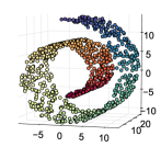
(a)

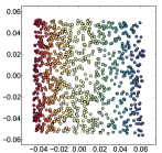
(b)

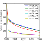
(c)

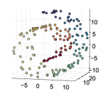
(d)

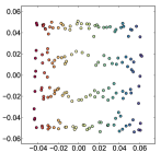
(e)

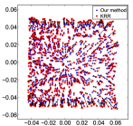
(f)

Figure 1: Results for a Swiss roll with $n=1000$ points: (a) the original 3D data points; (b) their 2D embedding; (c) the number of support vectors as a function of error tolerance $\varepsilon$ for various $\lambda$ and $\sigma$. For the remaining panels (d)-(f), we fix $\lambda=0.1$, $\sigma=4$, and $\varepsilon=0.003$: (d) the 161 support vectors found; (e) our approximated 2D embedding of support vectors; (f) a comparison of 2D embeddings from our method and kernel ridge regression (lines show correspondences).

We observe that the support vectors are not uniformly sampled in the input space nor on the learned 2D manifold. Instead, they appear along the boundaries or form a skeleton within the learned manifold. We also observe in Fig. 1LABEL:sub@fig:swiss-roll-comparison that the largest discrepancies in the predicted point locations between our sparse interpolator and kernel ridge regression occur along the boundaries. Unsurprisingly, increasing kernel width $\sigma$ reduces the number of support vectors needed to achieve the same error tolerance $\varepsilon$ as each support vector has broader spatial influence in the input space. Furthermore, increasing kernel ridge regression regularization parameter $\lambda$ also reduces the number of support vectors, as discussed in Section 3.

By repeating this experiment using a Swiss roll with $n=2000$, $n=3000$, and $n=4000$ points, we empirically find that for a variety of parameter settings $\lambda$, $\sigma$, and $\varepsilon$, the number of support vectors remains roughly constant as $n$ grows large. For example, with $\lambda=0.1$, $\sigma=4$, and $\varepsilon=0.003$, we obtain 161, 174, 163, and 170 support vectors for $n=1000,2000,3000,4000$ points respectively. This suggests that the number of support vectors to depend on the low-dimensional embedding’s complexity and not on the dataset size $n$.

4.2 Respiratory Gating of Ultrasound Images

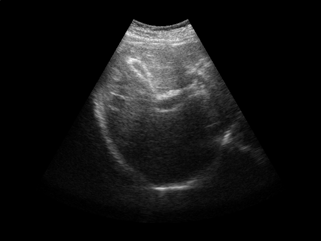
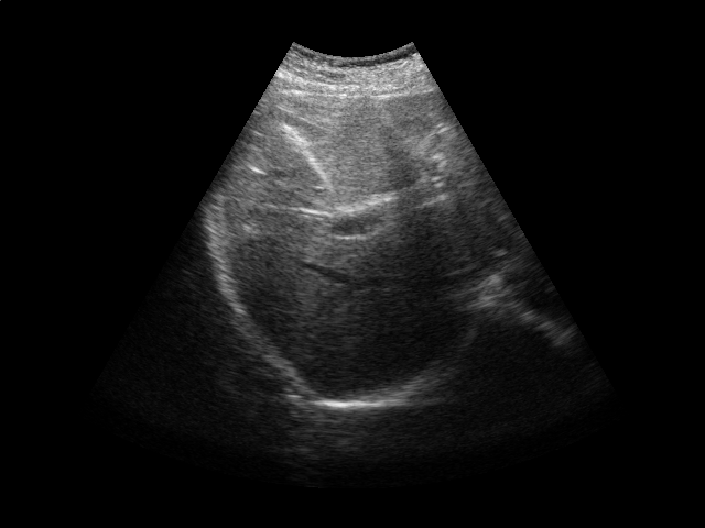
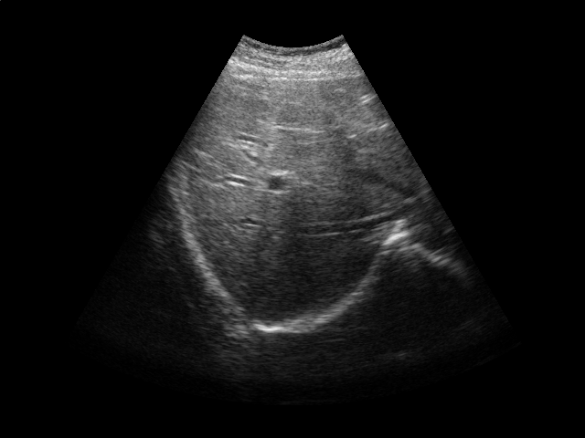
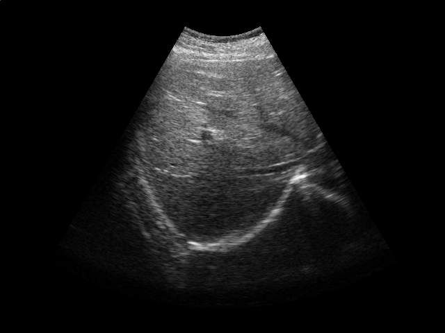
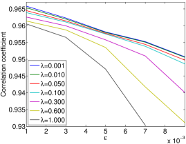
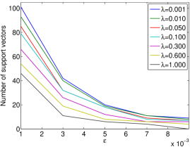
Figure 2: Ultrasound gating. Top: Ultrasound images of the liver over time (abdomen, right upper quadrant). Bottom left: Correlation coefficient vs. error tolerance $\varepsilon$. Bottom right: The number of support vectors vs. error tolerance $\varepsilon$. Both figures in the bottom report results for different values of kernel ridge regression regularization parameter $\lambda$.

		Learning on first 200 frames			Learning on entire data
Data	# Frames	CC (KRR)	CC (sparse)	# SV’s	CC (KRR)	CC (sparse)	# SV’s
Seq. 1	354	96.5%	96.4%	79	99.9%	96.9%	73
Seq. 2	335	97.7%	97.5%	99	99.9%	98.6%	100
Seq. 3	298	98.3%	97.8%	51	99.3%	98.9%	61
Seq. 4	371	99.7%	99.4%	53	99.6%	99.7%	45
Seq. 5	298	99.0%	98.7%	41	99.9%	99.5%	50

Table 1: Results for respiratory gating on ultrasound images. For each image sequence, we show the number of frames it contains, the correlation coefficient (CC) for kernel ridge regression (KRR) and our sparse interpolator, and the number of support vectors (SV’s). Parameter values: $\lambda=0.1$, $\varepsilon=0.001$.

Respiratory gating tracks a patient’s breathing cycle, which has numerous applications such as 4D imaging, radiation therapy, and image mosaicing [16]. Manifold learning has been used for highly accurate respiratory gating of ultrasound images [23], where 4D data reconstruction was achieved with retrospective gating, i.e., the gating was calculated after the data acquisition was finished. We extend this work to attain real-time gating. A small number of breathing cycles are acquired and used as input for manifold learning to construct the respiratory signal, as is done for retrospective gating. The new incoming stream of ultrasound images is then gated by performing an out-of-sample extension.

We conduct experiments on five 2D ultrasound image sequences of the human liver acquired during free breathing; example images are shown in Fig. 2. Each sequence contains 640$\times$480-pixel images and vary in length between 298 and 371 frames captured at 33 Hz. For a given image sequence, we use each image in the sequence as an input data point for learning a 1D manifold with Laplacian eigenmaps [4]; we use a 9-nearest-neighbor graph with an associated heat kernel of temperature $t=10$. The 1D embedding learned using an entire sequence of images serves as a reference signal for evaluating our sparse out-of-sample extension versus kernel ridge regression as the baseline. In what follows, we compare the 1D embedding of our sparse out-of-sample extension to the reference signal by computing a correlation coefficient between them. We use kernel ridge regression as a baseline method. Here we train on the first 200 frames and test on the remaining frames. We then compare the results with those obtained by training on all frames, as would be done for retrospective gating.

We first examine the influence of parameters $\varepsilon$ and $\lambda$ on the resulting interpolator. Training on the first 200 images of one of the ultrasound image sequences, we compute the correlation coefficient with the reference signal and the number of support vectors versus the error tolerance $\varepsilon$ (Fig. 2). As expected, smaller error tolerance $\varepsilon$ requires more support vectors but also leads to a higher correlation coefficient with respect to the reference signal. Also, a higher kernel ridge regression regularization parameter $\lambda$ leads to fewer support vectors. However, stronger regularization also leads to lower correlation coefficients. These results suggest a natural tradeoff between the accuracy and the computational cost of the projection operation.

In the next experiment, we use $\lambda=0.1$ and $\varepsilon=0.001$. Training on the first 200 frames and testing on the rest of the frames, we report the correlation coefficients and the number of support vectors in Table 1. The number of support vectors for kernel ridge regression is 200 in this case. We then repeat the experiment, training on all the frames. In this case, the number of support vectors for kernel ridge regression is the length of the sequence. We achieve a high correlation for all sequences, with a comparable performance between our sparse interpolator and kernel ridge regression. Comparing the number of support vectors when training on the first 200 frames vs. training on all the frames, we note that the number of support vectors stays roughly the same for a given image sequence. This again suggests that the number of support vectors depends on the low-dimensional embedding’s complexity and not the training set size.

4.3 Patient Position Estimation Using MRI

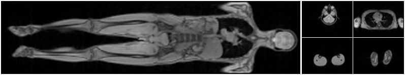
Figure 3: Left: Coronal plane of MRI scan showing the entire patient. Right: Axial slices on which manifold learning is performed.

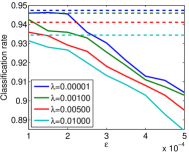
(a)

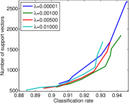
(b)

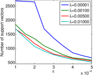
(c)

Figure 4: Leave-one-out classification results for MRI data: (a) classification rate vs. $\varepsilon$ for our sparse out-of-sample extension (solid line) and kernel ridge regression (dotted line) (b) the number of support vectors vs. classification rate; (c) the number of support vectors vs. error tolerance $\varepsilon$. All figures report results for different values of kernel ridge regression regularization parameter $\lambda$.

The radio frequency power in magnetic resonance imaging leads to tissue heating and has to be monitored by measuring the specific absorption rate, which depends on the position of the patient in the scanner. For current high-resolution scanners, this imposes restrictions because either fewer slices can be acquired or the in-plane resolution has to be reduced. Manifold learning can be used to estimate the position of the patient in the scanner [22].

First, low-resolution images are acquired while the bed that the patient lies on moves inside the scanner. The images are embedded in a low-dimensional space, where each axial image is associated with a body part (head, neck, lung, etc.) using a nearest-neighbor classifier. By knowing which slices correspond to which body parts, we can estimate the position of the patient in the scanner. It is important that the estimation be done in real-time to provide the position information before the high-resolution scan starts. In this application, we can apply manifold learning offline on a large database of scans. Then during the actual scan, we use an out-of-sample extension to project the acquired slices into the low-dimensional space. For large training datasets, it may be difficult to meet the time requirements with kernel ridge regression. Consequently, the reduction to a small set of support vectors offers a substantial advantage.

We run experiments on 13 whole body scans, such as the example shown in Fig. 3. A medical expert assigned an anatomical label (head, neck, lung, abdomen, upper leg, and lower leg) to each of the axial slices (64$\times$64 pixels). We apply Laplacian eigenmaps to embed the high dimensional slices in a two-dimensional space; we use a 40-nearest-neighbor graph with a heat kernel of temperature $t=49$. To predict the anatomical label of an axial image, we perform nearest-neighbor classification in the learned low-dimensional space. We repeat this classification procedure for different values of error tolerance $\varepsilon$ ranging from $1\times 10^{-4}$ to $5\times 10^{-4}$.

We compare the classification performance of embeddings obtained from our sparse interpolator and kernel ridge regression. Fig. 4LABEL:sub@fig:MRa reports leave-one-out classification performance for different values of error tolerance $\varepsilon$. The classification rates for kernel ridge regression are provided for comparison; they do not change for different values of $\varepsilon$. Figs. 4LABEL:sub@fig:MRb and 4LABEL:sub@fig:MRc characterize the sparsity of the interpolation function constructed by reporting the number of support vectors as a function of the classification rate and error tolerance $\varepsilon$. The total number of frames used in this experiment is 2697, which corresponds to the number of support vectors for kernel ridge regression. We observe a clear correlation between error tolerance $\varepsilon$ and the classification performance. Smaller values of $\varepsilon$ lead to better classification performance but require more support vectors. Thus, we can trade off computational speed with classification performance by tuning parameters $\lambda$ and $\varepsilon$ to be as large as possible while maintaining a classification rate above a minimum tolerated threshold.

5 Conclusion

We derived a novel method for multivariate regression that approximates kernel ridge regression, where the final estimated interpolation function depends only on a subset of the original input points acting as support vectors. Our approach provides a guarantee on the approximation error for training data. We applied our method as an out-of-sample extension for manifold learning, illustrating applications to respiratory gating and MRI classification.

Turning toward nonlinear dimensionality reduction more generally, many widely used algorithms are computationally expensive for massive datasets. Thus, ideally we would like to find support vectors first, before applying dimensionality reduction. Our results suggest that the support vectors for interpolation may not be uniformly sampled in the input space. This invites the question of how to non-uniformly sample training data in the input space and adjust a dimensionality reduction algorithm accordingly to account for the geometry of these samples.

Acknowledgements. We thank Siemens Healthcare for image data. This work was funded in part by the National Alliance for Medical Image Computing (grant NIH NIBIB NAMIC U54-EB005149) and the National Institutes of Health (grants NIH NCRR NAC P41-RR13218 and NIH NIBIB NAC P41-EB-015902).

References

- [1] Aronszajn, N.: Theory of reproducing kernels. Trans. AMS (1950)
- [2] Bach, F.R., Jenatton, R., Mairal, J., Obozinski, G.: Optimization with sparsity-inducing penalties. Foundations and Trends in Machine Learning (2012)
- [3] Beck, A., Teboulle, M.: A fast iterative shrinkage-thresholding algorithm for linear inverse problems. SIAM Journal on Imaging Sciences (2009)
- [4] Belkin, M., Niyogi, P.: Laplacian eigenmaps and spectral techniques for embedding and clustering. In: NIPS (2002)
- [5] Bengio, Y., Paiement, J.F., Vincent, P., Delalleau, O., Roux, N.L., Ouimet, M.: Out-of-sample extensions for LLE, Isomap, MDS, eigenmaps, and spectral clustering. In: NIPS (2004)
- [6] Bhatia, K.K., Rao, A., Price, A.N., Wolz, R., Hajnal, J.V., Rueckert, D.: Hierarchical manifold learning. In: MICCAI (2012)
- [7] Cawley, G.C., Talbot, N.L.C.: Reduced rank kernel ridge regression. Neural Processing Letters (2002)
- [8] Donoho, D.L., Grimes, C.: Hessian eigenmaps: New locally linear embedding techniques for high-dimensional data. PNAS (2003)
- [9] Drucker, H., Burges, C.J.C., Kaufman, L., Smola, A.J., Vapnik, V.: Support vector regression machines. In: NIPS (1997)
- [10] Georg, M., Souvenir, R., Hope, A., Pless, R.: Manifold learning for 4d ct reconstruction of the lung. In: CVPR Workshops (2008)
- [11] Gerber, S., Tasdizen, T., Joshi, S., Whitaker, R.: On the manifold structure of the space of brain images. In: MICCAI (2009)
- [12] Hamm, J., Davatzikos, C., Verma, R.: Efficient large deformation registration via geodesics on a learned manifold of images. In: MICCAI (2009)
- [13] van der Maaten, L.J.P., Postma, E.O., van den Herik, H.J.: Dimensionality reduction: A comparative review. Tilburg University Technical Report (2008)
- [14] Natarajan, B.K.: Sparse Approximate Solutions to Linear Systems. SIAM J. Comput. (1995)
- [15] Rohde, G.K., Wang, W., Peng, T., Murphy, R.F.: Deformation-based nonlinear dimension reduction: Applications to nuclear morphometry. In: ISBI (2008)
- [16] Rohlfing, T., Maurer, Jr., C.R., O’Dell, W.G., Zhong, J.: Modeling liver motion and deformation during the respiratory cycle using intensity-based free-form registration of gated MR images. In: Medical Imaging: Visualization, Display, and Image-Guided Procedures (2001)
- [17] Roweis, S.T., Saul, L.K.: Nonlinear dimensionality reduction by locally linear embedding. Science (2000)
- [18] Saunders, C., Gammerman, A., Vovk, V.: Ridge regression learning algorithm in dual variables. In: ICML (1998)
- [19] Schölkopf, B., Smola, A.J.: Learning with Kernels: Support Vector Machines, Regularization, Optimization, and Beyond. MIT Press (2001)
- [20] Suzuki, K., Zhang, J., Xu, J.: Massive-training artificial neural network coupled with laplacian-eigenfunction-based dimensionality reduction for computer-aided detection of polyps in ct colonography. IEEE TMI (2010)
- [21] Tenenbaum, J.B., de Silva, V., Langford, J.C.: A global geometric framework for nonlinear dimensionality reduction. Science (2000)
- [22] Wachinger, C., Mateus, D., Keil, A., Navab, N.: Manifold learning for patient position detection in MRI. In: ISBI (2010)
- [23] Wachinger, C., Yigitsoy, M., Navab, N.: Manifold learning for image-based breathing gating with application to 4D ultrasound. In: MICCAI (2010)
- [24] Zhang, Q., Souvenir, R., Pless, R.: On Manifold Structure of Cardiac MRI Data: Application to Segmentation. CVPR (2006)