Probing Dust Settling in Proto-planetary Disks with ALMA

Abstract

Investigating the dynamical evolution of dust grains in proto-planetary disks is a key issue to understand how planets should form. We identify under which conditions dust settling can be constrained by high angular resolution observations at mm wavelengths, and which observational strategies are suited for such studies. Exploring a large range of models, we generate synthetic images of disks with different degrees of dust settling, and simulate high angular resolution ($\sim$ 0.05-0.3”) ALMA observations of these synthetic disks. The resulting data sets are then analyzed blindly with homogeneous disk models (where dust and gas are totally mixed) and the derived disk parameters are used as tracers of the settling factor. Our dust disks are partially resolved by ALMA and present some specific behaviors on radial and mainly vertical directions, which can be used to quantify the level of settling. We find out that an angular resolution better than or equal to $\sim$ 0.1” (using 2.3 km baselines at 0.8mm) allows us to constrain the dust scale height and flaring index with sufficient precision to unambiguously distinguish between settled and non-settled disks, provided the inclination is close enough to edge-on (i $\geq$ 75^∘). Ignoring dust settling and assuming hydrostatic equilibrium when analyzing such disks affects the derived dust temperature and the radial dependency of the dust emissivity index. The surface density distribution can also be severely biased at the highest inclinations. However, the derived dust properties remain largely unaffected if the disk scale height is fitted separately. ALMA has the potential to test some of the dust settling mechanisms, but for real disks, deviations from ideal geometry (warps, spiral waves) may provide an ultimate limit on the dust settling detection.

Stars: formation — stars: circumstellar matter — ISM: dust

1 Introduction

Grain growth and dust settling are two key ingredients in the planetary system formation process. Recent observational evidences suggest that ISM dust grains start to grow in the early phase of star formation, as soon as dense pre-stellar cores begin to form. Theory and numerical simulations predict that in Class II proto-planetary disks, the dust orbiting the Pre-Main-Sequence (PMS) star continues to grow but also very quickly settles along the mid-plane in typical characteristic time of a few $10^{4}$ yrs (Dullemond & Dominik 2004; Fromang & Nelson 2009). The growth is the first step towards the formation of even larger solid bodies, which ultimately culminate with planetary embryos. Settling will speed up this process by favouring grain collisions, firstly by increasing the relative vertical velocities, as settling acts differently in function of the dust dynamic properties (see e.g. Birnstiel et al. 2010), and secondly by concentrating dust close to the midplane. On top of that, a high dust to gas ratio in this area, can affect the gravitational stability and control the initial step of the formation of planetesimals (Goldreich & Ward 1973).

Quantifying the dust evolution process is a complex problem since the two physical processes (grain growth and dust settling) are simultaneously shaping the disk. The big grains are expected to fall down relatively quickly to the mid-plane while only small grains, reflecting the stellar light (Burrows et al. 1996; Roddier et al. 1996), should remain located on the disk surface, at 3-5 gas scale heights.

At a radius of 100 AU from the central star, typical hydrostatic scale heights range between 10-20 AU or $\sim 0.1^{\prime\prime}$ at the distance of the nearest low-mass star forming regions (D$\sim 140$ pc). Therefore, observing settling requires both the most sensitive and the most resolving astronomical facilities.

Some evidence of dust settling has been obtained from studies using Near-Infrared (NIR) maps obtained by the HST (Duchêne et al. 2003), or by the analysis of the Silicate band at 10$\mu$m (Pinte et al. 2008; D’Alessio et al. 2001). IR observations only characterize grain growth for small particles with sizes $a\sim 0.1-10~{}\mu$m, as images at wavelength $\lambda$ are mostly sensitive to particles of size $a\simeq\lambda/(2\pi)$. Moreover, as the dust opacity in the NIR is still quite large, the particles we observe are necessarily located high above the disk plane, typically around 3-5 scale heights (Chiang & Goldreich 1997).

Contrary to IR, the moderate opacity of the mm/submm domain should probe material throughout the disk structure. The early bolometric observations of envelopes and disks around young stars (Beckwith et al. 1990) indicated that both the dust absorption coefficient $\kappa_{\nu}$ and its spectral index $\beta$ at mm wavelengths have evolved compared to the ISM dust. However, only spatially resolved observations could alleviate the ambiguity left by the possible contribution of the inner optically thick core. Furthermore, contamination of the long wavelengths (longer than 4 mm) flux density by free-free emission can be substantial and should be removed for proper determination of the spectral index (Rodmann et al. 2006). Using the VLA (at 7 mm), PdBI and OVRO to probe the dust properties and the dust disk surface density in CQ Tau, Testi et al. (2003) concluded that particle have grown up to sizes as large as $\sim 1$ cm. Similar results were obtained on larger samples in $\rho$ Oph (with ATCA) and in Taurus-Auriga by Ricci et al. (2010b, a). The overall grain growth in proto-planetary disks thus seems a well establish fact.

More recently, Guilloteau et al. (2011) performed a high angular resolution dual frequency study of disks in the Taurus-Auriga region with the IRAM array. Apart from disks with inner holes such as LkCa15 (Piétu et al. 2006), all sources observed with sufficiently high angular resolution (0.4-0.8^′′) exhibit steeper brightness gradient at 3 mm than at 1.3 mm. This is the signature of an evolution of the dust spectral index with radius, with smaller $\beta$ values near the central star. The inner part of disks, up to 60-80 AU, appears dominated by large particles leading to a spectral index $\beta$ below 0.5 between $\lambda=3$ and 1.3 mm while beyond 100 AU, $\beta$ reaches value consistent with ISM-like grains (1.7). This constitutes the first observational evidence of radial variations in dust properties, and the characteristic transition radius between small and large grains is consistent with recent models of dust evolution in disks by Birnstiel et al. (2010).

In this paper, we go one step further and study the impact of dust settling on the disk imaging at mm wavelengths, in order to define adequate observational strategies to constrain this phenomenon with ALMA. For this purpose, we utilize the code DISKFIT (Piétu et al. 2007), which has been upgraded to take into account the dust settling. The ALMA simulator developed at IRAM (Pety et al. 2002) is then used to generate realistic ALMA datasets within the wavelength range 0.5 to 3 mm. Finally, we analyze these synthetic observations (pseudo-observations) as real data assuming a vertically uniform dust distribution in order to find out robust criteria of dust settling. We also explore some hidden degeneracies which may bias our estimate of the dust properties. We then discuss what would be an ideal ALMA observation.

Our dust disk models are described in Section 2. Section 3 presents the ALMA predictions (pseudo-observations) and the method of analysis. We then discuss in Section 4 the implications of our results.

2 Model Description

2.1 Disk Model

As in Guilloteau et al. (2011), we assume a simple parametric disk model. In Model 1, the gas surface density is a simple power law with a sharp inner and outer radius:

$$\Sigma_{g}(r)=\Sigma_{0}\left(\frac{r}{R_{0}}\right)^{-p},$$ (1)

for $R_{\mathrm{int}}<r<R_{\mathrm{out}}$.

In Model 2, the density is tapered by an exponential edge:

$$\Sigma_{g}(r)=\Sigma_{0}\left(\frac{r}{R_{0}}\right)^{-\gamma}\exp\left(-(r/R_{c})^{2-\gamma}\right).$$ (2)

Note that Model 1 derives from Model 2 by simply setting $R_{c}\rightarrow\infty$ and $p=\gamma$ in the above parametrization. Model 2 is a solution of the self-similar evolution of a viscous disk in which the viscosity is a power law of the radius (with constant exponent in time $\gamma$) (Lynden-Bell & Pringle 1974).

The kinetic temperature in the disk mid-plane is also assumed to be a power law of the radius:

$$T_{k}(r,z=0)=T_{0}(r/R_{0})^{-q}.$$ (3)

We assume that grains and gas are fully thermally coupled, so that the dust temperature $T_{\mathrm{dust}}=T_{k}$. We shall further assume that the disk is vertically isothermal, $T_{k}(r,z)=T_{k}(r,z=0)$. Models of dust settling show that most of the dust should mostly settle within one scale-height (Dullemond & Dominik 2004), therefore assuming that the dust is isothermal, is at first order a reasonable assumption. The impact of this assumption will be discussed later. Under hydrostatic equilibrium, the resulting vertical gas distribution is a Gaussian

$$\rho(r,z)=\frac{\Sigma(r)}{H_{g}(r)\sqrt{\pi}}\exp{\left(-\left(\frac{z}{H_{g}(r)}\right)^{2}\right)}.$$ (4)

With this definition, the gas scale height $H_{g}$ is:

$$H_{g}(r)=\sqrt{\frac{2r^{3}kT_{k}(r)}{GM_{*}\mu m_{H}}}$$ (5)

with $k$ and $G$ the Boltzmann and the gravitational constants respectively, $M_{*}$ the star mass, $\mu$ the mean molecular weight and $m_{H}$ the mass of the Hydrogen nuclei. $H_{g}$ is also a power law of the radius

$$H_{g}(r)=H_{0}(r/R_{0})^{h},$$ (6)

with the exponent $h=3/2-q/2$. The mean molecular weight $\mu$ is equal to 2.6 in our analysis.

2.2 Dust Properties

2.2.1 Mass and grain size distributions

Dust settling implies local changes in the dust-to-gas ratio, as well as local variations in the grain size distribution, whose details depend on the mechanism controlling the dust evolution. We assume here no radial re-distribution of dust: the dust surface density $\Sigma_{d}$ follows the gas surface density, and at any radius the average (i.e. vertically integrated) dust-to-gas ratio is equal to the standard ratio:

$$\Sigma_{d}(r)/\Sigma_{g}(r)=\zeta_{\mathrm{std}}=1/100$$ (7)

Eq.7 ensures mass conservation independently of settling. The value of $\zeta_{\mathrm{std}}$ is only a scaling factor for the total disk mass in non-settled disks, but also affects settling in some specific models.

We further impose that dust settling does not change the overall dust distribution as a function of grain size, and use a power law size distribution

$$\frac{\int\mathrm{d}n(a,r,z)dz}{\mathrm{d}a}=n_{0}\left(\frac{a}{a_{0}}\right)^{-{p_{d}}}~{}~{}~{}~{}~{}~{}a_{min}\leq a\leq a_{max}.$$ (8)

$n_{0}$ is the number of grains at the reference size $a_{0}$, $a_{min}$ and $a_{max}$ are the minimum and maximum radius of the particles and ${p_{d}}$ the exponent of the power law (usually taken from 2.5 to 4, e.g. Ricci et al. 2010b). While the vertically integrated grain size distribution is a power law (and a fortiori, the disk averaged grain size distribution), because of the effect of dust settling, the local grain size $n(a,r,z)$ distribution is no longer a power law of $a$.

2.2.2 Dust emissivity

The dust emissivity as a function of frequency depends on the dust size distribution and grain composition. Once the dust size distribution and grain composition are specified, several methods can be used to derive the emissivity values. This has to be done with grain sizes varying up to 5 to 6 orders of magnitude. A serious limitation is our poor knowledge of the grain composition and shape. Moreover, several recent observations and experiments show that the dust spectral index $\beta$ in the Far IR/mm range depends on the dust temperature (Pollack et al. 1994; Agladze et al. 1996; Coupeaud et al. 2011). The Mie theory is the most popular method (see, e.g. Draine 2006) to predict dust emissivities but remains rigorously exact for spherical grains only. Other methods, such as the Discrete Dipole Approximation (DDA), are heavier to handle (see, e.g. Draine 1988; Draine & Flatau 2012, and references therein) and still suffer from the dust composition and shape limitations.

One often uses approximate laws for the dust emissivity in the mm domain, such as a simple power law prescription $\kappa(\nu)=\kappa_{0}(\nu/\nu_{0})^{\beta}$. Although in general applicable to the molecular clouds where grains remain small, in disks, this approximation is only valid over a relatively narrow range of frequencies. Realistic disk grains can result in emissivity curves which cannot be represented in this way at mm wavelengths, especially when the largest grain become comparable in size to the wavelength (Natta et al. 2004; Ricci et al. 2010b; Isella et al. 2009). Furthermore, in settled disks, such a representation would no longer be convenient, as relating the effective $\kappa_{0}$ and $\beta$ to the dust settling parameters is a non trivial task. Thus a 2-D (r,z) distribution of the dust emissivity as a function of wavelength needs to be computed once the settling parameters are specified.

Given the important unknowns in the dust geometry and composition, we have elected to use a parametric method to model the dust emissivity as a function of grain size and wavelength.

Our approach is based on the fact that the emissivity as a function of frequency displays two asymptotic regimes, the small wavelengths ($a\gg\lambda$) where the absorption coefficient is dictated by the geometrical cross section, and the long wavelengths ($a\ll\lambda$) for which a power law applies. These two regimes are connected by a resonance region near $\lambda=2\pi a$. To study the thermal structure of disks, Inoue et al. (2009) parameterized the emissivity curves by only retaining the two asymptotic laws. However, at mm wavelengths, the resonant region can contribute significantly to the emissivity. The detailed behaviour of this resonant region is not critical, as integration over a size distribution will smooth out any fine structure: only the width and height matter. We thus elected to parameterize the asymptotic regimes and the width and height of this resonant region in a simple way. The details are given in Appendix A.

To integrate over a given distribution in size, the distribution is sampled on discrete bins. We typically use two (logarithmic) bins per decade in size, except for the smallest sizes (below 1$\mu$m) where 1 bin per decade is used because these small grains contribute very little to the emissivity at mm wavelengths (and are also less affected by settling effects). Within each bin, the size distribution is assumed to remain a power law with the same exponent ${p_{d}}$ as the integrated grain size distribution. Our selected functional for the emissivity $\kappa(\nu,a)$ allows analytic integration over this truncated power law size distribution to derive the mean emissivity per unit mass.

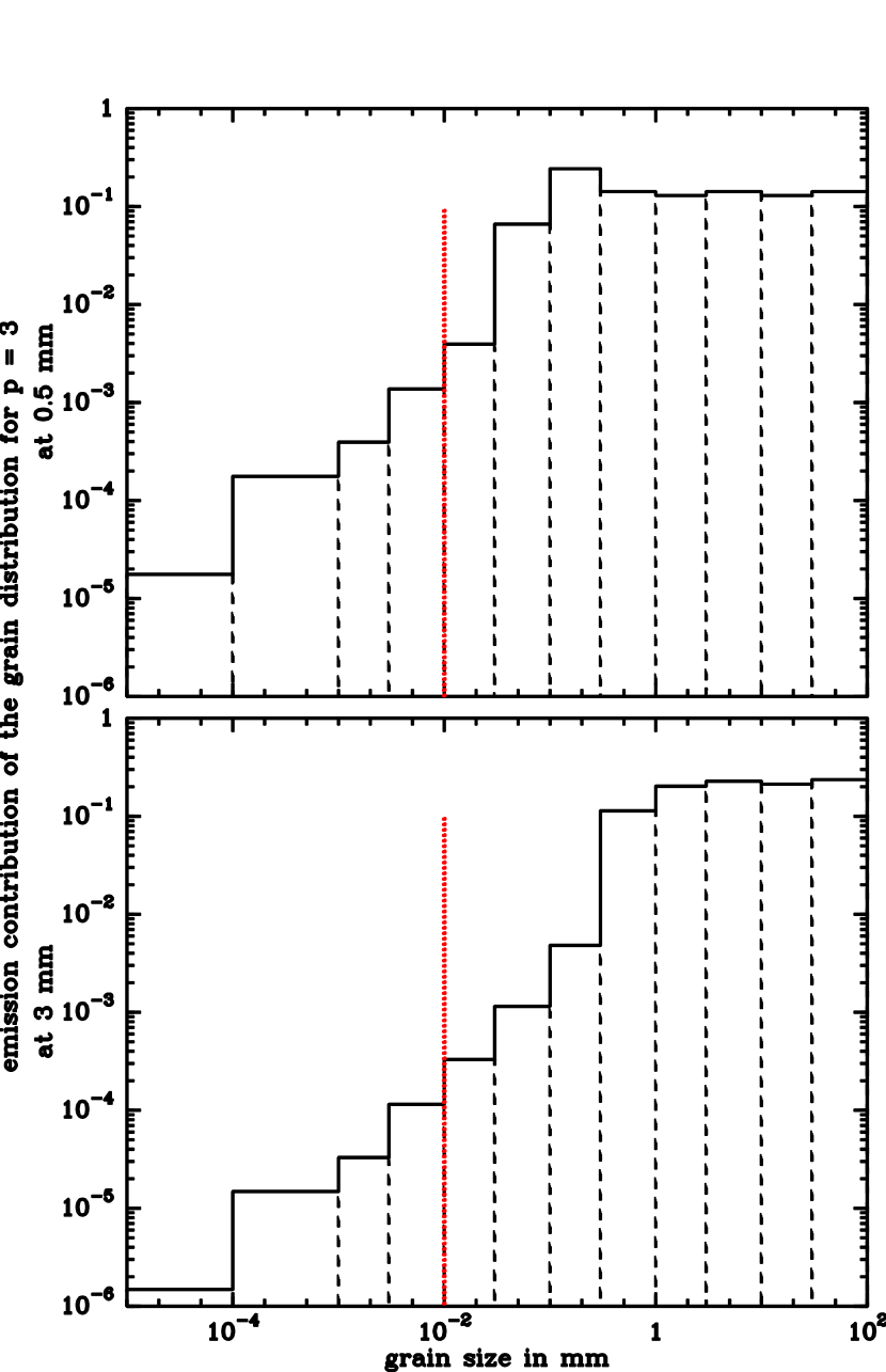
Figure 1: Contribution of various dust grains to the total emission (at 3 and 0.5mm wavelengths), depending of their size, for an assumed size exponent ${p_{d}}=3$. The vertical red dotted line represents approximately (depending of disk density) the separation between grains well mixed with the gas and grains starting to settle.

In the example presented in this article, the parameters have been adjusted in order to match the dust properties used by Ricci et al. (2010b). The resulting emissivity per size bin are given in Table 1, and Fig.1 shows the relative contribution of each bin to the total emission, for a size distribution index ${p_{d}}$   equal to 3.

Table 1: Dust Emissivity calculated from our simplified model.

grain size		$\kappa$ (cm2g-1)
$a_{-}$	$a_{+}$	0.5 mm	0.8 mm	1.3 mm	3 mm
0.01$\mu$m	30 $\mu$m	8.33	3.80	1.69	0.418
30 $\mu$m	100 $\mu$m	40.1	7.69	1.84	0.418
0.1 mm	0.3 mm	51.4	34.5	11.1	0.610
0.3 mm	1 mm	8.60	8.74	9.52	4.12
1 mm	3 mm	2.75	2.75	2.58	2.58
3 mm	10 mm	0.860	0.860	0.826	0.826
10 mm	30 mm	0.275	0.275	0.270	0.270
30 mm	100 mm	0.0860	0.0860	0.0860	0.0859

2.3 Dust Settling

Although dust settling mechanism does not in general lead to a Gaussian vertical distribution of grains of a given size $a$, this often remains an acceptable approximation. Deviations from such vertical profile only occurs high above the typical scale height, i.e. in regions which contribute very little to the total dust mass (see e.g. Fromang & Nelson 2009).

It is convenient to define a grain-size dependent scale height, $H_{d}(a,r)$, and a “settling factor”, $s(a,r)=H_{d}(a,r)/H_{g}(r)$ with $a$ being the grain size. In our binned dust representation, a radius independent dust settling can be simulated by specifying the values of $s_{n}=s(a_{n})$ for each bin. A two-bin representation (one layer of large grains, close to the mid-plane, and one of small, near the disk surface) is also used by D’Alessio et al. (2006) to study the impact of dust settling on disk SED. A small difference is that in D’Alessio et al. (2006) the two grain categories are spatially separated, while in our case they would only have different scale heights.

To obtain the s(a,r) value, we decided to use instead a more physical approximation based on the results of global numerical calculations derived from theoretical approaches (Fromang & Nelson 2009) which take into account ideal MRI-induced MHD turbulence predictions (Balbus & Hawley 1991, 1998) as well as vertical stratification of dust and gas.

In a Keplerian disk, the angular velocity is:

$$\Omega=\Omega_{0}\left(\frac{r}{R_{0}}\right)^{-3/2}$$ (9)

and relates to the scale height in hydrostatic equilibrium by:

$$\Omega=\sqrt{2}\frac{C_{s}}{H_{g}}$$ (10)

were $C_{s}$ is the (isothermal) sound speed. The dust stopping time is the typical time, for a particle of size $a$ and density $\rho_{d}$, initially at rest to reach the local gas velocity. In typical T Tauri protoplanetary disks, aerodynamic interactions between gas and solid particules smaller than $\sim$ 10 meters are well described by the Epstein regime (Garaud et al. 2004). We have then for the dust stopping time the expression:

$$\tau_{s}=\frac{\rho_{d}a}{\rho C_{s}}$$ (11)

The main factor controlling the degree of settling is the dimensionless product of the dust stopping time $\tau_{s}$ by the angular velocity which fixes the dynamical time. When $\Omega\tau$ $\ll$ 1, the dust particles are coupled to the gas. When $\Omega\tau$ $\gg$ 1, the dust particles are decoupled from the gas and settles towards the midplane. This product is linked to the particle size $a$ by:

$$\Omega\tau_{s}(r,z)=\frac{\sqrt{2\pi}\rho_{d}a}{\Sigma_{g}(r)}\exp{(z/H_{g}(r))^{2}}$$ (12)

where the surface density $\Sigma_{g}(r)$ is given by Eqs.1-2, depending on which disk model is used. As this quantity is therefore inversely proportional to the gas surface density, in general the settling increases with radius.

It is convenient to further approximate the effects of dust settling by relating the “settling factor” $s(a,r)$ to the settling parameter $\Omega\tau_{0}=(\Omega\tau_{s})(r,z=0)$:

$$s(a,r)=\frac{H_{d}(a,r)}{H_{g}(r)}=f\left(\Omega.\tau_{0}\right)$$ (13)

For large grains, Dubrulle et al. (1995) and Carballido et al. (2006) have shown that a power law:

$$s(a,r)=\frac{H_{d}(a,r)}{H_{g}(r)}=\left(\Omega.\tau_{0}\right)^{\sigma}$$ (14)

with $\sigma=-0.5$ is a suitable function. With a similar representation, Pinte et al. (2008) found an exponent $\sigma=-0.05$ from a multi-wavelength study of IM Lupi. However, their value is mostly constrained by infrared data, and more specifically the silicate bands which are essentially sensitive to small grains. We have adopted the following law, which matches the previous asymptotic results

$$s(a,r) = 1\hskip 49.79231pt\mathrm{if}\quad{}\Omega\tau_{0}<\omega_{c}$$ (15)

$$= \left(\frac{\Omega\tau_{0}}{\omega_{c}}\right)^{-0.5}\hskip 14.22636pt\mathrm{if}\quad{}\Omega\tau_{0}>\omega_{c}$$

where $\omega_{c}\approx\alpha$, the viscosity parameter, within a factor of order unity (Dubrulle et al. 1995). From Fig.2, we use in red $\omega_{c}=6.5\,10^{-4}$, a value which slightly overestimates the settling efficiency found by Fromang & Nelson (2009). We will also discuss in Sec. 4.4.2 of the value $\omega_{c}=1.7\,10^{-3}$, in blue, which on contrary tends to underestimate it. For small grains, the small difference between our adopted exponent of 0 for small $\Omega\tau$ and the value -0.05 found by Pinte et al. (2008) is unimportant for our purpose, since the emission in the mm/submm domain is largely dominated by grains affected by dust settling, as illustrated by Fig.1.

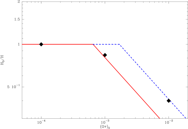
Figure 2: Dust scale height as a function of $(\Omega.\tau_{s})_{0}$ (adapted from Fromang & Nelson 2009). The black diamonds represent the values calculated by the simulations. The red and dashed blue lines indicate the two functions adopted in our study.

2.4 Radiative Transfer

We used the ray-tracer of the radiative transfer code DISKFIT (Piétu et al. 2007) to generate brightness distributions at different wavelengths. As settling can only be observed at sufficiently high disk inclinations, special care was taken in defining the image sampling to limit the numerical effects, as described in Guilloteau et al. (2011). This required to have radial and vertical cells smaller than 0.05 AU.

3 Simulations

3.1 Sample of Disk Models

Table 2: Disk physical parameters for a 1$\,\mathrm{M_{\odot}}$ star.

Physical characteristics	Adopted values
type of grains	Moderate ($\leq$ 3 mm)
	or Large ($\leq$ 10 cm)
gas scale height	Hydrostatic Equilibrium (Eq.5)
Averaged Gas/Dust	100
Kinetic Temperature	$T_{k}(r)=30\left(\frac{r}{R_{0}}\right)^{-0.4}$ Kelvin
Dust Temperature	$T_{dust}=T_{k}$
Reference radius	$R_{0}$ = 100 AU
Inner Radius	$R_{int}$ = 3 AU
Inclinations	70, 80, 85 and 90°
Gas Surface Density (g.cm-2)   Truncated disk (model 1, Eq.1)
$\Sigma_{g}(r)$	$4.35\left(\frac{r}{R_{0}}\right)^{-p}$
$p$	1
Outer edge	$R_{out}$ = 100 AU
Gas Surface Density (g.cm-2)   Viscous disk (model 2, Eq.2)
$\Sigma_{g}(r)$	$17.4\left(\frac{r}{R_{0}}\right)^{-\gamma}\mathrm{exp}\left(\-(\frac{R}{R_{c}})^{2-\gamma}\right)$
$\gamma$	0.5
Tapered edge	$R_{c}$ = 50 AU

The disks parameters (Table 2) are representative of the disks studied by Guilloteau et al. (2011). The disks are in hydrostatic equilibrium with no vertical temperature gradient and orbit around a $1$$\,\mathrm{M_{\odot}}$star. The total (gas+dust) disk mass is 0.03 $\,\mathrm{M_{\odot}}$.

3.1.1 Dust Settling and Emissivity

Table 3: Settling factors $s$ for the various grain size distributions

grain size		$s(a)=H_{d}/H_{g}$ at Radius (AU)
$a_{-}$	$a_{+}$	$R_{\mathrm{int}}=3$	50	$R_{\mathrm{out}}=100$
0.01 $\mu$m	10 $\mu$m	1.00	1.000	1.000
10 $\mu$m	30 $\mu$m	1.00	0.867	0.613
30 $\mu$m	100 $\mu$m	1.00	0.481	0.340
0.1 mm	0.3 mm	1.00	0.274	0.194
0.3 mm	1 mm	0.621	0.152	0.108
1 mm	3 mm	0.354	0.0867	0.0613
3 mm	10 mm	0.196	0.0481	0.0340
10 mm	30 mm	0.112	0.0274	0.0194
30 mm	100 mm	0.0621	0.0152	0.0108

The settling factor $s$ is calculated for $p_{d}=3$, $\rho_{d}=1.5$ g.cm^-3 with $a$ corresponding to the mean (mass weighted) grain radius, and the disk model described in Table 2.

We simulate the settling using the prescription of Eq.15. Table 3 gives the corresponding settling factors and Fig.3 indicates the apparent scale height for various grain sizes as a function of radius.

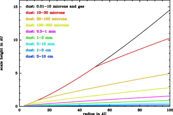
Figure 3: Dust and gas scale heights as a function of the radius for different grain sizes for the settled model. The black curve also corresponds to the gas scale height.

Following the formalism described in Section 2.2, dust parameters were adjusted to mimic the emissivity curves from Ricci et al. (2010b), see Appendix A. The minimum grain size was 0.01 $\mu$m and the maximum grain size 3 mm for the moderate grain model or 10 cm for the large grain model, with $p_{d}=3$. We took 9 grain bins for the moderate grains and 12 for the large ones for ensuring sufficient precision at the ALMA noise level. While compact minerals have large specific densities of $\rho_{d}=3-4$ g.cm^-3, we have chosen to use a smaller value $\rho_{d}=1.5$ g.cm^-3 to account for the fact that (large) grains are expected to harbor a substantial ice cover and to be fluffy. The resulting emissivities are given in Table 1.

3.1.2 Gas Surface Densities

The gas surface density used to generate the settled disk model follows either Eq.1 (power law model, Model 1) or Eq.2 (viscous model, Model 2). Fig.4-5 were obtained using the Model 1. Tables 5 and 6 correspond to pseudo-observations using the Model 1. In Table 7 and 8, the pseudo observations were obtained using the Model 2. The resulting integrated flux densities are given in Table 4.

Table 4: Flux densities (mJy) of settled disks (Model 1)

Frequency	100 GHz	230 GHz	340 GHz	670 GHz
Moderate grains
70°	65	450	989	3490
80°	48	300	634	2100
85°	32	180	377	1240
90°	7.6	56	137	564
Large grains
70°	9.6	60	134	512
80°	9.0	56	123	462
85°	8.1	49	107	393
90°	2.4	17	39	166

3.1.3 ALMA Configuration

The simulated brightness distributions obtained from DISKFIT were then processed through the regularly upgraded ALMA simulator implemented in the GILDAS software package (Pety et al. 2002) in order to produce the visibilities.

As a first guess, we choose to simulate observations obtained using 50 antennas with a single antenna configuration, so that observations at different wavelengths can be performed nearly simultaneously. A maximum baseline length of 2.3 km was used and the observations were assumed to be around the transit. Pseudo-observations of settled disks, located at declination $\delta=-23^{\circ}$, have been created at four different frequencies, 100, 230, 340 and 670 GHz (or in wavelengths: 3 mm, 1.3 mm, 0.88 mm and 0.48 mm, corresponding to the 4 initial ALMA bands 3,6,7 and 9). This leads to a spatial resolution of 0.30^′′, 0.13^′′, 0.089^′′ and 0.045^′′ for Bands 3,6,7 and 9, respectively. At the distance of the nearest star forming regions (120 – 140 pc for $\rho$ Oph and Taurus-Auriga), the corresponding linear resolutions are 39-42, 16-18, 11-12 and 5-6 AU. In our case, we assume a distance of 140 pc. Thermal noise was added to the simulated $uv$ data (corresponding to 30 min of observations for each frequency). The resulting image noise (point source sensitivity) are 13 $\mu$Jy at 100 GHz, 20 at 230 GHz, 30 at 340 GHz and 111 at 670 GHz.

Each disk has been imaged at 4 inclination angles ($90^{\circ}$, $85^{\circ}$, $80^{\circ}$ and $70^{\circ}$). The resulting number of visibilities in the pseudo $uv$ tables is 1096704. This number can be compared to the non reduced $\chi^{2}$ given in Tables 5 to 8.

3.2 Prominent Effects of Settling

To understand the effect of settling, it is useful to compare the images of the same disk (i.e. having the same gas spatial distribution and mass) with or without settling.

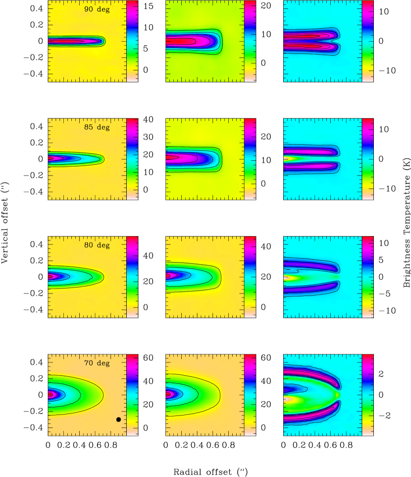
Figure 4: Disks observed at 670 GHz under inclinations of 90^∘, 85^∘, 80^∘ and 70^∘, from top to bottom. Left: settled disks. Middle: non-settled disks of same gas mass distribution and same amount of dust. Right: difference between these two models (non settled - settled). Simulations are made with moderate grains. The hatched ellipse is the PSF.

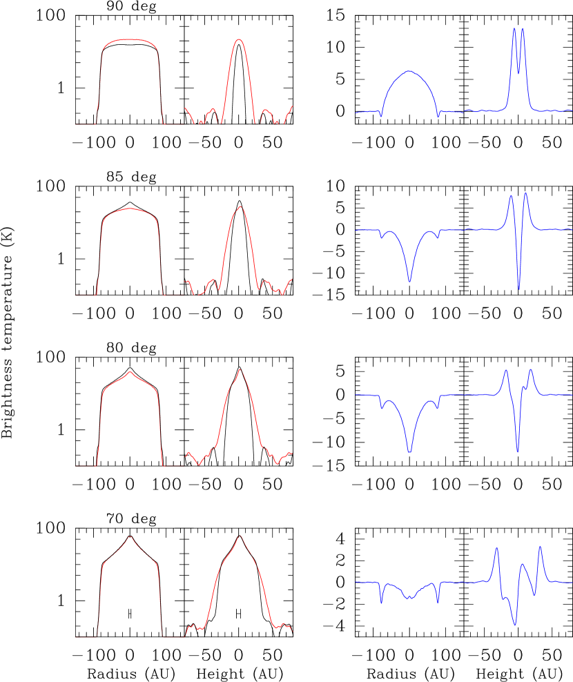
Figure 5: Radial and vertical cuts in brightness temperature distribution (K) of disks with moderate grains, observed at 670 GHz under different inclinations. Left: black curves correspond to the settled model. Red curves correspond to the non-settled model. Right: the differences (non settled - settled) between these two models is shown in blue. The horizontal bar indicates the angular resolution.

Figure 4 represents the expected images for disks observed at 670 GHz, while Fig. 5 gives brightness profiles for cuts along and perpendicular to the disk midplane at the disk center.

As expected, the vertical extent is smaller in the settled case, as well as the flaring index. At very high inclinations (only at 90^∘ in our model), the $\tau$ $=$ 1 region of settled disks is reached at larger radial distances from the star, which are colder. This results in a lower brightness temperature.

We find the same effect with large grains: their lower absorption coefficient is partially compensated by higher column densities in the mid-plane due to stronger settling. The self-absorption effect will be smaller for less massive disks. Thus, a change in disk mass and a modification of the grain sizes result in different effects, in particular as a function of observing frequency.

Finally, because the intrinsic aspect ratio is of order H/R $\leq$ 0.1, these opacity effects are critically dependent on the inclination (see Figs 4 and 5). At 70^∘, the impact of dust settling becomes in general difficult to see.

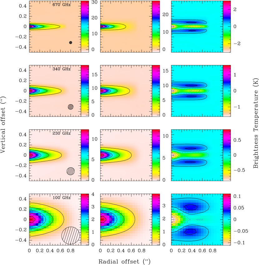
Figure 6: Left: settled disks at 85^∘ of inclination. Middle: results of the best model obtained with the non-settled disk model (Case 1). Right: difference between these two models (non settled - settled). Models are made with large grains. The hatched ellipse is the PSF.

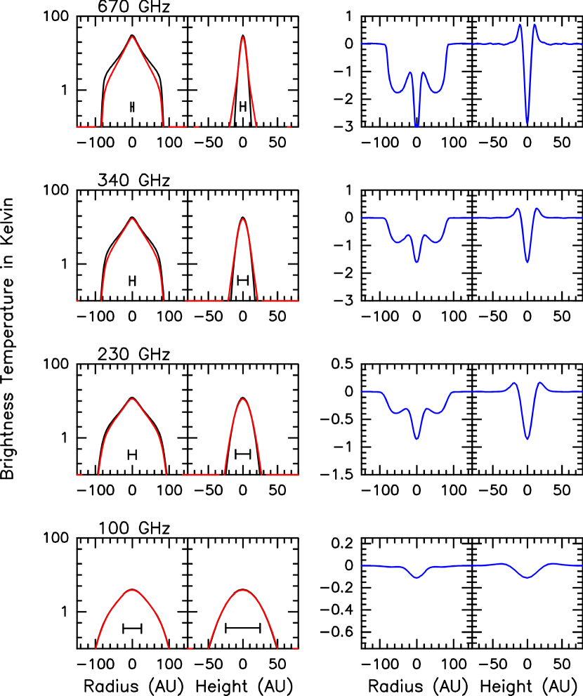
Figure 7: Radial and vertical cuts in brightness temperature distribution (K) at several wavelengths for disks inclined at $85^{\circ}$ and large grains corresponding to Fig.6. Left: black curves correspond to the settled model. Red curves correspond to the non-settled model. Right: the differences (non settled - settled) between these two models is shown in blue. The horizontal bar indicates the angular resolution.

3.3 Inversion Process

We investigate here potential ways to distinguish any settled disk from any non-settled one. Our approach is to analyze simulated images of settled disks with non-settled, homogeneous disk models. Under this approach, settled disks may result in very unusual parameters which cannot be ascribed to “normal” non-settled disks. For example, the dust scale height $H_{0}$ should be small, as well as the flaring index $h$, in comparison with the hydrostatic scale height.

The resulting $uv$ data sets were fitted by non-settled and vertically isothermal models under the assumption of power law (Model 1, Eq.1) or exponential decay (Model 2, Eq.2) for the surface density distribution. All frequencies were fitted simultaneously. Tables 5, 6 and 8 were obtained with minimizations performed using the Model 1 and Table 7 using the Model 1 and Model 2).

Table 5: Minimizations of a settled disk (model 1) by an homogeneous one (model 1): moderate size grains

Disk Case &	$T_{0}$	$q$	$p$	$R_{\mathrm{out}}$	$\beta_{i}$	$\beta_{r}$	$H_{0}$	$h$	$\chi^{2}$
inclination	30 K	0.4	1.0	100 AU	0.613	0	14.6 AU	1.30
(Case 1)
70∘	30.3 $\pm$ 0.08	0.396 $\pm$ 0.001	0.966 $\pm$ 0.002	95.8 $\pm$ 0.02	0.613 $\pm$ 0.001	[0]	(14.7)	(1.30)	$1458941$
80∘	33.8 $\pm$ 0.07	0.378 $\pm$ 0.002	1.32 $\pm$ 0.004	96.1 $\pm$ 0.03	0.420 $\pm$ 0.001	[0]	(15.5)	(1.31)	$1696971$
85∘	26.6 $\pm$ 0.10	0.629 $\pm$ 0.007	0.692 $\pm$ 0.006	97.9 $\pm$ 0.04	0.341 $\pm$ 0.002	[0]	(13.7)	(1.18)	$1661490$
90∘	18.8 $\pm$ 0.22	0.810 $\pm$ 0.035	-1.20 $\pm$ 0.03	101.0 $\pm$ 0.07	0.892 $\pm$ 0.005	[0]	(11.6)	(1.10)	$1332034$
(Case 2)
70∘	30.3 $\pm$ 0.08	0.396 $\pm$ 0.001	0.965 $\pm$ 0.006	95.8 $\pm$ 0.02	0.612 $\pm$ 0.002	0.000 $\pm$ 0.005	(14.7)	(1.30)	$1458923$
80∘	33.8 $\pm$ 0.13	0.378 $\pm$ 0.001	1.32 $\pm$ 0.01	96.1 $\pm$ 0.03	0.420 $\pm$ 0.003	0.003 $\pm$ 0.008	(15.5)	(1.31)	$1697294$
85∘	26.4 $\pm$ 0.17	0.640 $\pm$ 0.005	1.16 $\pm$ 0.01	98.4 $\pm$ 0.06	0.230 $\pm$ 0.003	-0.23 $\pm$ 0.01	(13.7)	(1.18)	$1660374$
90∘	19.3 $\pm$ 0.3	0.622 $\pm$ 0.013	0.55 $\pm$ 0.07	102 $\pm$ 0.10	0.440 $\pm$ 0.005	-1.21 $\pm$ 0.02	(11.7)	(1.19 )	$1325182$
(Case 3)
70∘	28.3 $\pm$ 0.04	0.423 $\pm$ 0.001	1.09 $\pm$ 0.005	99.7 $\pm$ 0.007	0.686 $\pm$ 0.001	[0]	2.55 $\pm$ 0.05	1.06 $\pm$ 0.016	1205325
80∘	29.2 $\pm$ 0.03	0.412 $\pm$ 0.001	1.43 $\pm$ 0.009	99.7 $\pm$ 0.009	0.704 $\pm$ 0.002	[0]	2.49 $\pm$ 0.04	0.94 $\pm$ 0.007	1193405
85∘	30.2 $\pm$ 0.03	0.391 $\pm$ 0.001	0.27 $\pm$ 0.06	100. $\pm$ 0.03	0.682 $\pm$ 0.007	[0]	2.91 $\pm$ 0.06	1.18 $\pm$ 0.03	1155545
90∘	31.2 $\pm$ 0.19	0.39 $\pm$ 0.034	-1.20 $\pm$ 0.05	101. $\pm$ 0.07	0.833 $\pm$ 0.007	[0]	3.06 $\pm$ 0.05	-0.09 $\pm$ 0.02	1117094
(Case 4)
70∘	28.1 $\pm$ 0.04	0.425 $\pm$ 0.001	1.22 $\pm$ 0.008	99.8 $\pm$ 0.007	0.648 $\pm$ 0.002	-0.080 $\pm$ 0.005	2.49 $\pm$ 0.06	1.05 $\pm$ 0.014	1205325
80∘	29.1 $\pm$ 0.03	0.415 $\pm$ 0.001	1.78 $\pm$ 0.02	99.8 $\pm$ 0.008	0.644 $\pm$ 0.003	-0.21 $\pm$ 0.02	2.52 $\pm$ 0.04	0.97 $\pm$ 0.007	1192868
85∘	30.2 $\pm$ 0.03	0.391 $\pm$ 0.001	0.35 $\pm$ 0.09	100 $\pm$ 0.06	0.601 $\pm$ 0.007	-0.46 $\pm$ 0.07	2.95 $\pm$ 0.07	1.26 $\pm$ 0.03	1155401
90∘	30.2 $\pm$ 0.19	0.54 $\pm$ 0.038	-1.65 $\pm$ 0.09	101 $\pm$ 0.07	0.897 $\pm$ 0.006	0.17 $\pm$ 0.02	3.05 $\pm$ 0.06	-0.11 $\pm$ 0.03	1117059

Numbers between brackets $[]$ indicate fixed parameters. Numbers between parentheses are derived from another parameter ($H_{0}$ from $T_{k}$ and $h$ from $q$ under the hydrostatic equilibrium hypothesis). The second row indicates the expected values of the parameters. See section 3.3 for the definition of Cases.

Non-settled disks are characterized by the following parameters: the position angle PA, the inclination $i$, the intrinsic parameters $R_{\mathrm{int}},R_{\mathrm{out}},\Sigma_{0}~{}\mathrm{and~{}}p$ (for the power law, $R_{c},\gamma$ for the viscous model), $T_{0},q$, $H_{0},h$ and the dust characteristics. The later being a priori unknown, we assume the simple power law $\kappa(\nu)=\kappa_{0}(\nu/\nu_{0})^{\beta}$ for the dust emissivity. We use here $\nu_{0}=10^{12}$ Hz and $\kappa_{0}=0.1$ cm²g^-1 (for a dust to gas ratio of 1/100). As $\beta$ is a free parameter in our analysis, the choice of $\nu_{0}$ will affect $\kappa(\nu)$ at other frequencies, which is compensated in our analysis by adjusting the disk density. The derived disk density profiles $\Sigma(r)$ (and in particular the disk mass) is thus somewhat dependent on the assumed value of $\nu_{0}$.

Each pseudo-observation was fitted with 4 different non-settled disk models. The scale height was derived either under hydrostatic equilibrium constraint or independently fitted, and dust emissivity exponent $\beta$ was assumed to be independent of the radius $r$, or evolving like its logarithm:

$$\beta(r)=\beta_{i}+\beta_{r}\log(r/R_{0})$$ (16)

This leads to 4 cases (see Tables 5-6). Case 1 assumes hydrostatic equilibrium and $\beta_{r}=0$, Case 2 hydrostatic equilibrium and free $\beta_{r}$, while Case 3 uses free scale height $H_{0}$ and $h$ with $\beta_{r}=0$ and Case 4 all free parameters $H_{0},h$ and $\beta_{r}$. As the impact on $R_{\mathrm{int}}$ was found to be non significant in all cases, this parameter is ignored thereafter. The disk inclination $i$ is recovered accurately in all cases (with typical error around 0.2°), but its knowledge controls the error bars on some critical parameters, in particular $H_{0}$ and $h$. The position angle is also easily recovered, but has less influence than the inclination.

Table 6: Minimizations of a settled disk (model 1) by an homogeneous one (model 1): large grains

Disk Case &	$T_{0}$	$q$	$p$	$R_{\mathrm{out}}$	$\beta_{i}$	$\beta_{r}$	$H_{0}$	$h$	$\chi^{2}$
inclination	30 K	0.4	1.0	100 AU	0.288	0	14.6 AU	1.30
(Case 1)
70∘	22.2 $\pm$ 1.2	0.453 $\pm$ 0.014	0.92 $\pm$ 0.013	99.1 $\pm$ 0.2	0.337 $\pm$ 0.004	[0]	(12.6)	(1.27)	1099461
80∘	19.2 $\pm$ 0.6	0.555 $\pm$ 0.011	0.78 $\pm$ 0.01	96.5 $\pm$ 0.2	0.366 $\pm$ 0.004	[0]	(11.7)	(1.23)	1103372
85∘	17.8 $\pm$ 0.3	0.668 $\pm$ 0.010	0.70 $\pm$ 0.01	95.8 $\pm$ 0.2	0.464 $\pm$ 0.005	[0]	(11.2)	(1.17)	1115798
90∘	11.9 $\pm$ 0.4	0.967 $\pm$ 0.055	-0.82 $\pm$ 0.06	96.6 $\pm$ 0.3	0.98 $\pm$ 0.02	[0]	(9.1)	(1.02)	1113205
(Case 2)
70∘	15.0 $\pm$ 1.0	1.10 $\pm$ 0.04	-0.07 $\pm$ 0.04	99.8 $\pm$ 0.1	0.45 $\pm$ 0.008	0.126 $\pm$ 0.004	(10.3)	(0.95)	1099558
80∘	13.8 $\pm$ 0.9	1.30 $\pm$ 0.017	-0.45 $\pm$ 0.02	97.9 $\pm$ 0.2	0.50 $\pm$ 0.007	0.182 $\pm$ 0.004	(9.9)	(0.85)	1102652
85∘	17.7 $\pm$ 0.24	0.674 $\pm$ 0.010	0.73 $\pm$ 0.02	95.8 $\pm$ 0.2	0.45 $\pm$ 0.008	-0.01 $\pm$ 0.01	(11.2)	(1.17)	1114358
90∘	13.0 $\pm$ 0.35	0.660 $\pm$ 0.027	0.73 $\pm$ 0.08	97.8 $\pm$ 0.2	0.43 $\pm$ 0.02	-0.93 $\pm$ 0.05	(9.6)	(1.17)	1112144
(Case 3)
70∘	32.0 $\pm$ 1.0	0.40 $\pm$ 0.02	1.01 $\pm$ 0.02	99.6 $\pm$ 0.06	0.266 $\pm$ 0.004	[0]	1.6 $\pm$ 0.7	1.43 $\pm$ 0.13	1097745
80∘	33.0 $\pm$ 0.9	0.35 $\pm$ 0.02	1.08 $\pm$ 0.02	98.9 $\pm$ 0.2	0.270 $\pm$ 0.004	[0]	1.9 $\pm$ 0.5	0.68 $\pm$ 0.07	1098468
85∘	33.9 $\pm$ 1.0	0.32 $\pm$ 0.02	1.13 $\pm$ 0.02	98.7 $\pm$ 0.2	0.268 $\pm$ 0.004	[0]	1.4 $\pm$ 0.2	0.53 $\pm$ 0.12	1099739
90∘	22.3 $\pm$ 0.8	1.49 $\pm$ 0.07	-1.34 $\pm$ 0.07	100. $\pm$ 0.2	0.51 $\pm$ 0.02	[0]	1.4 $\pm$ 0.2	0.03 $\pm$ 0.07	1096614
(Case 4)
70∘	27.8 $\pm$ 1.3	0.510 $\pm$ 0.05	0.84 $\pm$ 0.08	99.7 $\pm$ 0.06	0.30 $\pm$ 0.01	0.027 $\pm$ 0.006	1.1 $\pm$ 0.3	1.3 $\pm$ 0.4	1097740
80∘	35.9 $\pm$ 1.3	0.310 $\pm$ 0.03	1.17 $\pm$ 0.03	98.9 $\pm$ 0.14	0.23 $\pm$ 0.01	-0.028 $\pm$ 0.005	1.6 $\pm$ 0.6	0.6 $\pm$ 0.2	1098426
85∘	34.5 $\pm$ 1.1	0.309 $\pm$ 0.03	1.20 $\pm$ 0.03	98.8 $\pm$ 0.2	0.22 $\pm$ 0.01	-0.043 $\pm$ 0.007	1.3 $\pm$ 0.2	0.45 $\pm$ 0.2	1099695
90∘	58.0 $\pm$ 3.1	-0.28 $\pm$ 0.03	1.64 $\pm$ 0.08	100. $\pm$ 0.2	0.11 $\pm$ 0.01	-0.64 $\pm$ 0.05	1.3 $\pm$ 0.2	0.05 $\pm$ 0.1	1096561

4 Discussion

4.1 Analysis of the Inversion Process

Tables 5-8 show the results of the inversion process. In Tables 5 and 6, both pseudo-observations and models for the minimizations use the truncated disk surface density (Model 1), with grains of moderate size in Table 5 and large grains in Table 6. In Table 7, pseudo-observations, made with the viscous Model 2 and containing large grains, are analysed by both Models 1 and 2. Finally, Table 8 refers to pseudo-observations obtained with Model 1 and fitted using the Model 2, for moderate size grains.

The case with grains of moderate size illustrates best the problems. It leads to rather strong continuum flux (Table 4), and the optically thick zone is sufficiently large to measure directly the dust temperature from the surface brightness. The formal errors are very small, indicating that thermal noise is not a limitation here.

Table 7: Tapered Edge disk: large grains

Disk Case &	$T_{0}$	$q$	$p$	$R_{\mathrm{out}}$	$\beta_{i}$	$\beta_{r}$	$H_{0}$	$h$	$\chi^{2}$
inclination	30 K	0.4			0.288	0	14.6 AU	1.30
70∘
(Case 1)	32.9 $\pm$ 0.1	0.310 $\pm$ 0.001	1.73 $\pm$ 0.002	91.7 $\pm$ 0.07	0.689 $\pm$ 0.002	[0]	(15.3)	(1.35)	1151874
(Case 2)	29.8 $\pm$ 0.07	0.348 $\pm$ 0.001	2.16 $\pm$ 0.004	92.9 $\pm$ 0.07	0.419 $\pm$ 0.004	-0.322 $\pm$ 0.004	(14.6)	(1.33)	1141912
(Case 3)	28.7 $\pm$ 0.11	0.379 $\pm$ 0.002	1.65 $\pm$ 0.002	94.1 $\pm$ 0.08	0.725 $\pm$ 0.002	[0]	20.0 $\pm$ 0.13	2.32 $\pm$ 0.007	1143237
(Case 4)	25.4 $\pm$ 0.07	0.426 $\pm$ 0.001	1.90 $\pm$ 0.006	94.0 $\pm$ 0.08	0.629 $\pm$ 0.005	-0.181 $\pm$ 0.004	18.4 $\pm$ 0.14	2.31 $\pm$ 0.009	1134115

As Table 5 for a viscous (model 2) settled disk fitted by an homogenous disk with sharp edge (model 1).

Disk Case &	$T_{0}$	$q$	$p$	$R_{c}$	$\beta_{i}$	$\beta_{r}$	$H_{0}$	$h$	$\chi^{2}$
inclination	30 AU	0.4	0.5	50 AU	0.288	0	14.6 AU	1.30
70∘
(Case 1)	30.5 $\pm$ 0.09	0.387 $\pm$ 0.001	0.479 $\pm$ 0.003	49.3 $\pm$ 0.04	0.620 $\pm$ 0.002	[0]	(14.7)	(1.31)	1106571
(Case 2)	29.6 $\pm$ 0.08	0.391 $\pm$ 0.001	0.578 $\pm$ 0.003	46.2 $\pm$ 0.09	0.536 $\pm$ 0.003	-0.092 $\pm$ 0.002	(14.5)	(1.30)	1106488
(Case 3)	25.1 $\pm$ 0.10	0.473 $\pm$ 0.002	0.459 $\pm$ 0.003	51.2 $\pm$ 0.05	0.682 $\pm$ 0.002	[0]	3.4 $\pm$ 0.3	1.73 $\pm$ 0.03	1099314
(Case 4)	25.3 $\pm$ 0.09	0.463 $\pm$ 0.002	0.520 $\pm$ 0.003	49.2 $\pm$ 0.09	0.628 $\pm$ 0.004	-0.052 $\pm$ 0.002	2.9 $\pm$ 0.4	1.65 $\pm$ 0.04	1099013

As Table 5 for a viscous (model 2) settled disk fitted by an homogenous viscous disk (model 2).

4.1.1 Deriving the Scale Height

When viewed edge-on, the hydrostatic equilibrium assumption (cases 1 and 2) leads to unusual results. The derived temperature is forced towards low values to better mimic the small disk thickness ($\sim$ 19 K instead of 30 K). This is also true when minimizing a Model 1 by a Model 2 (Table 8). A side effect is an apparent radial dependency of the dust emissivity index ($\beta_{r}\neq 0$) which is due to the nonlinearity of the Planck function at low temperatures. Relaxing the hydrostatic equilibrium hypothesis (cases 3 and 4) allows us to recover the input temperature profile.

Tables 5, 6 and 8 also show that the constraint from the apparent thickness is less important than that from the dust temperature, so that the fitted scale height in the hydrostatic equilibrium hypothesis remains unduly large (Fig. 6 and Fig.7). This artificially creates a deficit of emission close to the mid-plane and an excess at high altitude. For cases 3 and 4, there is a lack of flaring at all at 90^∘: the settled disk is best fitted with a constant thickness. At less extreme inclinations, however, disks appear mildly flared. Not only $H_{0}$ is constrained, but the apparent flaring index $h$ also deviates quite significantly in the settled case from the initial value (1.3 in our model, a range between 1.1 – 1.5 being expected for most disks).

4.1.2 Spectral Index

Our settled disk are composed of several populations of grains. Each grain population has its own spectral index $\beta$. If the whole dust emission was optically thin and homogeneously distributed, a mean $\beta$ (defined as the spectral index between two wavelengths only: 0.5 and 3 mm) of $\sim 0.61$ for the moderate grains (Table 5) and $\sim 0.29$ for the large grains (Table 6) is expected from the opacity curves in Appendix A. The fitted $\beta$ is often different because $\beta$ is not an intrinsic parameter of the dust: our assumed dust properties cannot be represented by a single power law between 3 and 0.5 mm, but exhibit a more complex behaviour (see Appendix). The fitted $\beta$ is more affected for edge-on disks, because the flux densities at each frequency strongly depend on the degree of settling, thus affecting the relative weights of each observation.

4.1.3 Degeneracy between $\beta_{r}$ and $p$

At very high inclinations (e.g. 90^∘), settling increases the opacity in the disk plane. A fit of a constant $\beta$ ($\beta_{r}=0$) leads to a value of the exponent $p$ of the radial density profile driven towards negative values, to offer sufficient self-absorption from the cold outer regions. The independent fit of $H_{0}$ and its exponent $h$ (case 4) is not sufficient to compensate this effect. Although this suggests that viscous-like surface density profiles (see Eq.2) with negative $\gamma$ may better fit the images, this is not the case because such profiles drop too sharply after their critical radius $R_{c}$. Furthermore, there is some “hidden” degeneracy between $p$ and $\beta_{r}$ and the minimization process may converge towards one or the other solution.

Table 8: Tapered Edge disk: moderate size grains

Disk Case &	$T_{0}$	$q$	$p$	$R_{\mathrm{out}}$	$\beta_{i}$	$\beta_{r}$	$H_{0}$	$h$	$\chi^{2}$
inclination	30	0.4			0.613	0	14.6	1.30
(Case 1)
70∘	34.8 $\pm$ 0.07	0.319 $\pm$ 0.001	2.14 $\pm$ 0.002	103.0 $\pm$ 0.03	0.442 $\pm$ 0.001	[0]	(15.7)	(1.34)	1276606
80∘	35.0 $\pm$ 0.07	0.346 $\pm$ 0.002	1.85 $\pm$ 0.004	103.0 $\pm$ 0.03	0.292 $\pm$ 0.001	[0]	(15.8)	(1.33)	1415333
85∘	29.5 $\pm$ 0.13	0.504 $\pm$ 0.004	1.31 $\pm$ 0.006	109.0 $\pm$ 0.06	0.293 $\pm$ 0.003	[0]	(14.5)	(1.25)	1683039
90∘	19.9 $\pm$ 0.26	0.542 $\pm$ 0.008	0.16 $\pm$ 0.01	109.6 $\pm$ 0.09	0.930 $\pm$ 0.006	[0]	(11.9)	(1.23)	1319208
(Case 2)
70∘	35.5 $\pm$ 0.07	0.306 $\pm$ 0.003	2.05 $\pm$ 0.005	108 $\pm$ 0.03	0.484 $\pm$ 0.005	0.156 $\pm$ 0.003	(15.9)	(1.35)	1299320 **
80∘	34.8 $\pm$ 0.07	0.349 $\pm$ 0.004	1.70 $\pm$ 0.007	111 $\pm$ 0.03	0.483 $\pm$ 0.008	0.300 $\pm$ 0.005	(15.7)	(1.33)	1393296
85∘	28.6 $\pm$ 0.09	0.533 $\pm$ 0.005	1.35 $\pm$ 0.008	116 $\pm$ 0.05	0.334 $\pm$ 0.010	-0.016 $\pm$ 0.007	(14.3)	(1.23)	1679815
90∘	20.6 $\pm$ 0.15	0.550 $\pm$ 0.009	0.18 $\pm$ 0.02	111 $\pm$ 0.07	0.398 $\pm$ 0.021	-1.25 $\pm$ 0.013	(12.1)	(1.22)	1312764
(Case 3)
70∘	35.8 $\pm$ 0.1	0.306 $\pm$ 0.001	2.23 $\pm$ 0.002	106 $\pm$ 0.03	0.466 $\pm$ 0.001	[0]	13.4 $\pm$ 0.04	1.33 $\pm$ 0.005	1262191
80∘	35.0 $\pm$ 0.06	0.302 $\pm$ 0.002	2.26 $\pm$ 0.005	110 $\pm$ 0.03	0.365 $\pm$ 0.001	[0]	6.6 $\pm$ 0.05	1.19 $\pm$ 0.006	1187642
85∘	32.8 $\pm$ 0.08	0.320 $\pm$ 0.003	2.69 $\pm$ 0.009	122 $\pm$ 0.05	0.461 $\pm$ 0.002	[0]	2.8 $\pm$ 0.04	0.53 $\pm$ 0.006	1129793
90∘	29.2 $\pm$ 0.13	0.294 $\pm$ 0.012	0.20 $\pm$ 0.01	113 $\pm$ 0.06	0.754 $\pm$ 0.076	[0]	4.0 $\pm$ 0.04	0.10 $\pm$ 0.02	1162383
(Case 4)
70∘	35.9 $\pm$ 0.06	0.305 $\pm$ 0.002	2.14 $\pm$ 0.004	108 $\pm$ 0.04	0.493 $\pm$ 0.005	0.099 $\pm$ 0.003	13.3 $\pm$ 0.03	1.32 $\pm$ 0.008	1278814 **
80∘	33.5 $\pm$ 0.08	0.330 $\pm$ 0.003	2.25 $\pm$ 0.010	114 $\pm$ 0.04	0.372 $\pm$ 0.005	0.172 $\pm$ 0.007	5.57 $\pm$ 0.05	1.10 $\pm$ 0.005	1186973
85∘	32.4 $\pm$ 0.09	0.327 $\pm$ 0.005	2.68 $\pm$ 0.017	127 $\pm$ 0.06	0.451 $\pm$ 0.010	0.268 $\pm$ 0.02	2.35 $\pm$ 0.03	0.44 $\pm$ 0.007	1124899
90∘	34.4 $\pm$ 0.10	0.068 $\pm$ 0.004	1.21 $\pm$ 0.007	122 $\pm$ 0.05	0.738 $\pm$ 0.008	-0.380 $\pm$ 0.005	4.04 $\pm$ 0.03	0.34 $\pm$ 0.016	1145282

As Table 5 for a viscous (model 2) settled disk fitted by an homogenous disk with sharp edge (model 1). ** Results probably not converged, as their $\chi 2$ is greater than that of the simpler $\beta_{r}=0$ case.

4.1.4 Impact of the Surface Density Profile

Table 5 suggests that the scale height can be apparently constrained independently of the temperature profile even at moderate ($i=70^{\circ}$) inclination (basically all input parameters are recovered properly). This result is due to the assumed sharp truncation at $R_{\mathrm{out}}=100$ AU (Model 1). The apparent (projected) width of this sharp edge is a strong indicator of the actual disk thickness.

Table 7 shows results for pseudo-observations obtained with a more realistic continuous profile (Model 2, with $\gamma=0.5$ and $R_{c}=50$ AU). When fitted by a Model 1 (top panel of Table 7), the required scale height is large and the flaring index reaches non physical values of the order of 2.5. This is an attempt to fit the emission beyond the derived outer radius. On the contrary when fitted by a Model 2 (bottom panel), a small scale height is indeed recovered. This result indicates that at inclinations below $80^{\circ}$, the recovered scale height is sensitive to the exact shape of the surface density distribution, and cannot in general be determined accurately. Table 8 shows results of tapered disks (Model 2) fitted by a truncated power law for different inclinations (Model 1) and moderate size grains. At inclinations $>80^{\circ}$, the differences between the true disk density structure and the one assumed in the analysis do not significantly affect the derivation of the scale height. Other parameters, such as the temperature, are somewhat affected by the improper surface density profile rather than by settling.

4.1.5 Consequences

For the large grains models, the flux densities and the optical depths are lower. The same trends are found. Large grains settle more efficiently and the fitted scale height is even smaller than in the previous case. Since the optically thick core is small, some degeneracies start appearing between $T,q$ and $\Sigma,p$, as a purely optically thin emission only depends on $\Sigma T$ and $p+q$.

In all cases, the inconsistencies appearing when fitting by a standard, non-settled disk model, clearly flag the “observed” disk as being unusual, and combined with the low absolute values of the scale height ($\simeq 2-3$ AU), point towards dust settling as the only reasonable cause of the discrepancies. Moreover, settled disks actually appear “pinched” ($h<1$)  rather than flared ($h>1$). The above analysis also demonstrates that radius dependent settling as derived from MRI simulations and theoretical analysis can be distinguished from radius independent one, the later would not affect the flaring index value $h$. However, directly retrieving the settling factor $s(a,r)$ will remain largely model dependent, as this would imply to deconvolve from the grain size distribution $n(a)$, which remains unknown. Even with prior knowledge of $n(a)$, the strong smoothing resulting from this size distribution would severely limit the capability to retrieve $s(a,r)$ from $H(r)$.

Others parameters like $\beta$, $\beta_{r}$ or $p$ are sensitive to the dust settling at inclinations $\geq$ 80^∘ but can only serve as secondary indicators. In real data, the $\beta_{r}$ which deviates from its original value 0 at inclinations $>$ 80^∘ may be due either to dust settling or to radial variations of the grain properties (Guilloteau et al. 2011).

An inclination close to 90^∘ is clearly the more suitable case to study settling since opacity and brightness temperature effects are maximum. Taken into account the various uncertainties, in particular on the surface density and radial grain properties, our results suggest that observations of settling would be possible at inclinations $>75-80^{\circ}$.

4.2 Impact of the various Wavelengths

The above studies show that all the impact of dust settling is only in the effective scale height (Fig.8) and a priori we may expect that the highest frequency data, which has the highest spatial resolution, may be sufficient in itself. This must be moderated by a number of caveats, however. First, the best signal to noise depends on the dust properties and is not necessarily at the highest frequency. Second, the apparent (geometrically constrained) scale height must be compared to the hydrostatic scale height to prove settling. This implies that a) the (gas) temperature or the dust temperature as a proxy, should be known, and b) the stellar mass must also be constrained to a reasonable accuracy (to derive H_g, see Eq.5). In principle, the gas temperature can be retrieved by imaging thermalized lines. However, as most chemical models predict that simple molecules lies in a layer about 1-2 scale height above the disk plane (because of depletion on dust grains in the cold denser regions, see e.g. Semenov & Wiebe 2011), finding a suitable probe for the disk plane is not straightforward. In our approach, the dust temperature is derived by resolving the optically thick parts of the disk. With radial gradients of the dust emissivity index like found by Guilloteau et al. (2011) and predicted by simulations of Birnstiel et al. (2010), the proper identification of an optically thick core region requires at least 3 frequencies. Thus unless some gas temperature can be derived independently, a 3-wavelength study seems required to avoid ambiguities in identifying dust settling.

The relative ability of each of our 4 observing wavelengths can be evaluated. For the two shortest ones (0.5 and 0.8 mm), the errors on the derived parameters (e.g. $H_{0}$ and $h$) approximately scale as the wavelength. Since the signal-to-noise ratio is similar at both frequencies, the driving factor is the angular resolution. The errors then strongly increases for 1.3 mm, which no longer has sufficient resolution, while the 3 mm data are practically unable to provide any quantitative constraint. Good observing conditions at 0.8 mm data being much more frequent than at 0.5 mm, this wavelength may be the best compromise in term of sensitivity and angular resolution if only one wavelength can be observed.

We note that the error on $T_{0}$ in the combined analysis is lower than the simple weighted average of the 4 independent determinations which shows the gain in the multi-wavelength approach.

We finally made a last check at 3 mm on long baselines by using the Model 1 to produce pseudo-observations in the case of the moderate grain size distribution and assuming an inclination angle of 85^∘. Baseline lengths of $\sim$ 11 km provide an angular resolution of about 0.06^′′ or 8 AU, similar to that reached at 0.5 mm with the $\sim 2$ km baselines. We mimic 4 hours of observations. We analyzed the pseudo-observations using the non settled disk Model 1 and found that the scale height is marginally constrained with $H_{0}=2.2\pm 0.7$ AU and $h=1.16\pm 0.3$. This also barely differs (by $\sim 1.5\sigma$) from the 4 wavelength fit where we obtain $H_{0}=3.13\pm 0.03$ AU. The large errors at 3 mm are due to insufficient sensitivity. Thus, measuring the differential settling between 0.5 and 3 mm would be very time consuming.

Figure 8: Derived apparent scale heights and flaring index as a function of disk inclination. All results show viscous pseudo-observations (Model 2) fitted by truncated disks (Model 1), using grains of moderate size, with free scale height and radial dependent $\beta$ (case 4). Stars show results obtained with the strong dust settling prescription while filled symbol are obtained with the lowest one. The dashed lines indicate the expected hydrostatic scale height and flaring index for non-settled disks.

4.3 Comparison with other imaging simulations

Using the code MC3D, Sauter & Wolf (2011) have investigated dust settling by producing intensity maps of dust disks from 1.0 $\mu$m up to 1.3 mm. Their analysis differs from ours in three major points.

First, they only assume two dust grain distributions (small and large) following the parametrization proposed by D’Alessio et al. (2006). Their small grain population is ISM-like, the large grain distribution extends up to $a_{max}$ = 1 mm. This parametrization is similar to the 2-bin version of our radius independent settling models (Section 2). It is very well suited to study settling in the NIR and Mid-IR because of the high dust opacity but has a too small number of bins to properly mimic dust settling at mm wavelengths. The maximum grain size may not be sufficient, as shown for example in Fig.3 where the larger grains significantly contribute to the mm emissions. They also only use stronger settling parameters, with their large grain scale height smaller than the small grain one by factors 8, 10 or 12. This roughly corresponds to the settling factor in our large grain case, but the ratio is of the order of 3 for our less extreme grain sizes.

Second, they do not take into account the ALMA transfer function. This is adequate only with sufficient $uv$ coverage, which is not obtained with short integrations on very long baselines.

Third, and most importantly, they only compare the settled model with the non-settled disk in four positions. Such a method, optimized for IR data, does not use all the information contained in the maps or ALMA observations. Moreover, as the dust opacity is changing with the wavelength, the optimum positions should vary accordingly.

Given these differences, comparisons are not straightforward. As expected, we both find weaker flux and reduced flaring for highly inclined settled disks, but our method appears much more discriminant and applicable to a wider range of disk inclinations.

4.4 Critical discussion

4.4.1 Temperature Structure:

We assume that the temperature is vertically isothermal (as did Fromang & Nelson (2009)). In real disks, the temperature is expected to rise two or three scale heights above the disk plane. Dust settling will affect this temperature gradient which is mostly driven by the distribution of small to mid-size grains ($\sim$ 0.1 to 10 $\mu$m) because they control the opacity to incoming radiation. These grains exhibit only limited settling. Indeed, because the apparent scale height at mm wavelengths is a factor 3 to 4 times smaller than the hydrostatic scale height, more than 99 % of the mm flux is built in within one hydrostatic scale height, in which temperature gradients should be negligible. The location of the super-heated layer changes with dust settling, but not to the point where it will substantially ($\geq$ 50 %) affect the temperature within one pressure scale height.

Hasegawa & Pudritz (2011) have recently studied the effect of dust settling on the dust temperature using MC3D (Wolf 2003). At 5 AU from the star, they found that the dust temperature near the mid-plane (within $z\leq 0.3$  scale-height) is somewhat lower in a settled disk than in a well-mixed one (see their Fig.4). The super-heated layer appears however hotter (60 K instead of 40 K). The thickness of the impacted cold layer is around 0.5 AU, much too small even for the longest ALMA baselines. At the larger radii (50 to 100 AU) investigated in our study, the impact of dust settling on the temperature structure will be much less significant, because the temperature gradients scale with the dust opacity ($\propto 1/r$ in typical disks), as well as with incoming radiation flux ($\propto 1/r^{2}$).

Vertical temperature gradients are however expected to play a role in the apparent scale height at optical or NIR wavelengths. Indeed for HH30, Burrows et al. (1996) derived a much larger scale height from 2 $\mu$m scattered light using the HST than Guilloteau et al. (2008) from IRAM PdBI data: this is more likely a manifestation of temperature gradient than of dust settling.

4.4.2 Settling Shape and Viscosity Parameter:

We have tested a prescription of the settling which has been derived from MRI driven turbulence simulations from Fromang & Nelson (2009). These simulations span a limited range of $(\Omega\tau_{s})_{0}$, and Figure 2 suggests that other settling factors may be used. We also performed simulations with $\omega_{c}$ about twice larger (dashed blue curve on Fig.2), leading to smaller settling but without any major change in our results as can be seen on Fig.8. The dust scale heights are affected by at most 30-40 %, but are still strongly smaller than the gas ($\sim$ 3 AU instead of 15 at R = 100 AU for the grain range size 0.1-1mm) and still easily distinguished from the unsettled case. Furthermore, the settling degree is also directed linked to the dust specific density, which is generally assumed to be between 1 and 3 g.cm^-3. As our grains have a relatively low dust specific density (1.5 g.cm^-3), and then are more coupled to the gas, the dust settling degree we generally used can be considered as medium. The measurable effects on the apparent flaring index indicate that the settling produced by MRI can be distinguished, in some cases, from a radially constant settling. For instance, in the simulation from (Fromang & Nelson 2009), there is no dead zone, leading to an underestimate of the dust settling in the inner disk ($r<10$ AU).

Having measured $H_{d}/H_{g}$, it is tempting to directly quantify the viscosity parameter $\alpha$. When this ratio is inferior to 1, the settling efficiency is related to it by (Dubrulle et al. 1995; Carballido et al. 2006):

$$s(a,r)=\frac{H_{d}(a,r)}{H_{g}(r)}\approx\sqrt{\frac{\alpha}{\Omega.\tau}}.$$ (17)

However, we do not measure $H_{d}(a,r)/H_{g}(r)$ as a function of grain size, but only an ensemble averaged with an a priori unknown size distribution, and a weighting function depending on the dust emissivity as function of size and wavelength. Furthermore, $\Omega\tau$ scales as the inverse of the gas surface density, which varies by factor of a few across the disk radius. These two effects are difficult to separate from the direct impact of $\alpha$ in the above formula. Thus, $H_{d}/H_{g}$ strongly depends on many parameters and quantifying $\alpha$ in this way appears impracticable. This conclusion is unfortunately re-inforced by the large integration times which would be required to measure differential settling between 0.5 and 3 mm, a minimal step to attempt any correction from the grain size distribution.

Each grain size bin is assumed to follow a Gaussian shape vertical distribution. Deviation from Gaussianity are expected, as shown by Fromang & Nelson (2009) from their MRI simulations. However, as these deviations occur above two-three scale-heights, they play a minor role in the mm/submm results, like the temperature profile.

4.4.3 Disk Size:

We use a disk outer radius of 100 AU, or a similar characteristic size for the tapered-edge profile. This is consistent with the sizes found for disks in the Taurus Auriga or $\rho$ Oph regions (Guilloteau et al. 2011; Andrews et al. 2009, 2010). The median disk outer radius in Guilloteau et al. (2011) is 130 AU.

Guilloteau et al. (2011) also show that large grains are essentially located in the inner 70 to 100 AU. The existence of a radial gradient in the grain size distribution will affect the radial dependency of settling. The presence of smaller grains beyond 100 AU, as suggested by the observational results of (Guilloteau et al. 2011), will increase the apparent scale height there. These outer regions contribute to less than 10 to 30 % of the total flux, so this increased scale height will not mask the settling from the inner regions. If grain growth is maximal near the star, the settling will become more important in the inner regions. Thus, the radial gradient of grain size should increase the expected values of the flaring exponent $h$. While this reduces one of the signature of settling, the effect can easily be mitigated by a slightly modified analysis method, as the change in $h$ is correlated with the change in grain size. This is amenable to simple parametrization, at the expense of one additional parameter.

4.4.4 Disk Mass:

We adopted a disk mass of $M_{d}=0.03\,\mathrm{M_{\odot}}$ which corresponds to flux densities given in Table 4 and are similar to those of disks found in e.g. the Taurus region (a factor 2 larger for the small grain case and a factor 2 smaller for the large grain case). With enough sensitivity, it is preferable to observe disks with low fluxes for two reasons: 1) at mm wavelength, low flux densities can be a sign of larger grains ($a>\lambda$) which settle more efficiently and 2) low flux densities may indicate lower densities which decrease the coupling between gas and dust. In the “large grain” approximation, the settling factor $s$ scales as $\sqrt{M_{d}/a}$ (from Eq.11 and 14), while for optically thin emission, the flux density $S_{\nu}$ scales as $\kappa(a)M_{d}\approx M_{d}/a$, so that $s\propto\sqrt{S_{\nu}}$, the settling efficiency $1/s$ may actually be larger for disks with lower observed flux densities, unless these low flux values are just due to disks of similar intrinsic densities, but smaller outer radii.

4.4.5 Disk Radial Structure:

We performed a series of tests where we fit the settled model (using moderate and large grain size distributions) with a viscous law for the surface density (Model 2) by a non-settled model assuming a power law surface density (Model 1). The results of the minimization (Table 8) show that even if the limited knowledge of the density profile unavoidably affects the precision with which settling is constrained, it does not mask its existence. For disks inclined by more than 80^∘, the derived scale height and its flaring clearly exhibit the behavior expected in case of dust settling. This result is strongly encouraging, especially as the radial density profile of disks is still a debated issue.

4.4.6 Disk Geometry:

Small departures from perfect geometry and rotational symmetry, like warps and spiral patterns, may affect our ability to constrain the scale height. Mis-alignments between jets and disks by a 1-2^∘ (e.g., HH 30 Pety et al. 2006), and warps of similar magnitude (e.g. $\beta$ Pictoris, Mouillet et al. 1997) are known to exists. They may ultimately limit the apparent scale height to about $H/R\simeq 0.03$, which is comparable to our “normal” grain size case. The very strong settling predicted for large grains by the MRI turbulent model may be beyond reach because of this practical limitation.

Figure 9: Impact of the phase noise on the measurements of settling. Top: reduced $\chi^{2}$, middle: flaring index $h$, bottom: apparent scale height at 100 AU. Left panels are for the small grain case, and right panels for the big grain case. The truncated power law (model 1) is used. Crosses are for $i=70$°, and squares for $i=85$°. The horizontal lines indicate the expected values for un-settled disks, derived from the hydrostatic conditions.

4.4.7 Instrumental Effects:

We have shown that thermal noise is not a major limitation to measure dust settling. We investigated here the impact of atmospheric phase noise by adding antenna based, Gaussian distributed phase errors, as would be expected after radiometric phase correction. Figure 9 shows the impact on the results. As expected, the impact is much worse on the brightest sources (the small grain case). However, for reasonable observing conditions (antenna based rms noise below 30^∘), phase noise does not prevent the measurement of the scale height. The flaring index is more affected, but $h$ still shows significant deviations at 85^∘ of inclination.

5 Summary

We have studied how ALMA can be used to quantify the degree of dust settling in proto-planetary disks around T Tauri stars. We simulated settled disks using prescriptions for dust settling based on MRI driven viscosity. Using a parametric model to fit the predicted dust emission as a function of wavelength, we show to what extent settling can be constrained. Our main findings are

• For the characteristic dust disk sizes found by previous mm surveys, dust settling can be measured in typical disks with moderate integration times (of about 2 hours per source), using baselines of the order of 2 km at the distance of the nearest star forming regions (120 - 140 pc).

• This is possible only for disks more inclined than $\sim 75-80^{\circ}$.

• Unless the gas scale height can be independently derived, at least 3 frequencies are needed to unambiguously identify settling, by comparing the apparent scale height to the derived dust temperature.

• The 3 mm band, which is useful to constrain $\beta$, is less sensitive to settling than shorter wavelengths even on long baselines (11 km) and for longer integration times (4 hours). Thus, measuring the differential settling between 0.5 and 3 mm would be very time consuming.

• Phase noise should be below about 40^∘ to avoid smearing by limited seeing. Although the highest frequencies provide better angular resolution, this condition favors the 0.8 mm band as the preferred frequency to probe the apparent scale height.

• At the highest inclination ($>85^{\circ}$), the apparent radial dependency of the surface density is affected by dust settling. However, this effect is not a sufficient diagnostic.

• Other parameters, such as the radial dependency of the dust emissivity index, are not substantially altered by settling.

Our study was performed using a viscosity parameter $\alpha\sim 10^{-3}$. Although settling is expected to depend on $\alpha$, the dependency is weak ($\sqrt{\alpha}$), and other unknowns, in particular the grain size distribution but also the surface density, preclude an accurate determination of $\alpha$ based on the observation of settling only.

Acknowledgements:
We acknowledge Sebastien Fromang for useful discussions about his simulations. The ALMA simulations use the regularly upgraded ALMA simulator developed at IRAM in the GILDAS package. This research was supported by the CNRS/INSU programs PCMI, PNP and PNPS and ASA.

Appendix A Determination of the grain emissivity

Dust grain emissivities can be computed from their dielectric properties. However, as grain properties are poorly known in proto-planetary disks, strong assumptions about the grain characteristics (shape, composition, porosity, ice layer, …) have to be made for such purpose.

We follow instead a much simpler approach which takes into account the basic asymptotic behaviour of the dust absorption coefficient as a function of wavelength. For wavelengths $\lambda$ much smaller than the grain radius $a$, grains behave as optically thick absorbers. Hence, the absorption coefficient per unit mass is wavelength independent and

$$\kappa(\lambda,a)=\pi a^{2}/m_{g}=3/(4\rho_{d}a)$$ (18)

for spherical grains of specific density $\rho_{d}$. At the other extreme, for $\lambda\gg a$, the emission coefficient usually falls as:

$$\kappa(\lambda,a)\propto(1/\lambda)^{\beta}$$ (19)

where $\beta$ ranges between 1 or 2, depending on the grain composition but not on grain sizes.

In between, for $\lambda\approx 2\pi a$, the absorption coefficient exhibits a number of bumps, due to interferences between the refracted and diffracted rays. The detailed shape of absorption curve in this resonant region depend on grain structure (Natta et al. 2004). However, these detailed shapes will be smeared out when the absorption coefficient is computed for a size distribution of the grains, so its exact knowledge is unimportant provided the overall emissivity curve can be reproduced for realistic grain size distributions.

We thus define the emissivity curve through a small number of parameters. For a given grain radius $a$, the short wavelength regime is given by:

$$k_{s}(a)=\frac{3}{4\rho_{d}a}$$ (20)

from equation 18. The long wavelength regime is defined by $k_{l}$ and $e_{l}$, so that for $\lambda\gg a$,

$$\kappa(\lambda)=k_{l}\lambda^{e_{l}}$$ (21)

The two regimes intersect at

$$\lambda_{0}(a)=a\left(\frac{k_{s}(a)}{k_{l}}\right)^{1/e_{l}}$$ (22)

The enhanced emissivity (“bump”) is defined at $\lambda_{1}(a)=2\pi l_{1}a$ by an enhancement factor $f_{p}>1$ compared to the long wavelength asymptotic regime

$$\kappa(\lambda_{1}(a),a)=f_{p}k_{l}\left(\frac{\lambda_{1}(a)}{a}\right)^{e_{l}}=f_{p}k_{l}\left(2\pi l_{1}\right)^{e_{l}}$$ (23)

The shape around this region is defined by slopes $\pm e_{b}$ before ($\lambda<\lambda_{1}(a)$) and $e_{a}$ after ($\lambda>\lambda_{1}(a)$) the bump. The $\pm$ sign for $e_{b}$ occurs because in this parametrization, $\kappa(\lambda_{1}(a),a)$ can be smaller than the short wavelength asymptotic value $k_{s}(a)$ (see Fig.10). The emissivity law being a piecewise combination of power laws of $\lambda$ and $a$, integration over a power law size distribution for the grains is straightforward.

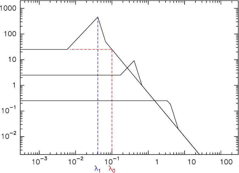
Figure 10: Absorption coefficient as a function $\lambda$ for three different size of grains(0.1, 1 and 10 mm). These curves correspond to $\rho_{d}=1.5$ g.cm^-3, long wavelength parameters exponent $e_{l}=-1.7$ and coefficient $k_{l}=0.5$ cm^0.3.g^-1 , and bump height $f_{p}=4$, exponents $e_{b}=1.5$, $e_{a}=-4.5$ and 98 position $l_{1}=0.65$.

This description with a limited number of parameters captures all the required characteristics to adequately represent the absorption curves of a given grain size distribution. Figure 11 shows the law used in our sample models, compared to the absorption coefficients used by Ricci et al. (2010b). The parameters are $f_{p}=15.4$, $e_{b}=0.68$, $e_{a}=-3.5$, $l_{1}=0.65$, $e_{l}=-1.67$ and $k_{l}=0.058$. Although differences by 20 % exist, the key features such as the asymptotic values, position width and height of the emissivity bump are all well reproduced.

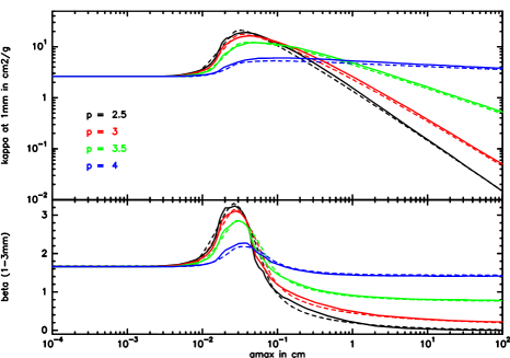
Figure 11: Top panel: Absorption coefficient $\kappa$ at 1 mm as a function of $a_{max}$ for different exponents $p$ of the size distribution. The solid lines represent the results calculated in Ricci et al (2010), using realistic grains made of astronomical silicates (10% in volume), carbonaceous materials (20%) and water ice. The dashed lines represent our approximated method. Bottom panel: emissivity exponent $\beta$ computed between 1 and 3 mm for the same grain distribution.

References

- Agladze et al. (1996) Agladze N. I., Sievers A. J., Jones S. A., Burlitch J. M., Beckwith S. V. W., 1996, ApJ, 462, 1026
- Andrews et al. (2009) Andrews S. M., Wilner D. J., Hughes A. M., Qi C., Dullemond C. P., 2009, ApJ, 700, 1502
- Andrews et al. (2010) Andrews S. M., Wilner D. J., Hughes A. M., Qi C., Dullemond C. P., 2010, ApJ, 723, 1241
- Balbus & Hawley (1991) Balbus S. A., Hawley J. F., 1991, ApJ, 376, 214
- Balbus & Hawley (1998) Balbus S. A., Hawley J. F., 1998, Reviews of Modern Physics, 70, 1
- Beckwith et al. (1990) Beckwith S. V. W., Sargent A. I., Chini R. S., Guesten R., 1990, AJ, 99, 924
- Birnstiel et al. (2010) Birnstiel T. et al., 2010, A&A, 516, L14+
- Burrows et al. (1996) Burrows C. J. et al., 1996, ApJ, 473, 437
- Carballido et al. (2006) Carballido A., Fromang S., Papaloizou J., 2006, MNRAS, 373, 1633
- Chiang & Goldreich (1997) Chiang E. I., Goldreich P., 1997, ApJ, 490, 368
- Coupeaud et al. (2011) Coupeaud A. et al., 2011, A&A, 535, A124
- D’Alessio et al. (2001) D’Alessio P., Calvet N., Hartmann L., 2001, ApJ, 553, 321
- D’Alessio et al. (2006) D’Alessio P., Calvet N., Hartmann L., Franco-Hernández R., Servín H., 2006, ApJ, 638, 314
- Draine (1988) Draine B. T., 1988, ApJ, 333, 848
- Draine (2006) Draine B. T., 2006, ApJ, 636, 1114
- Draine & Flatau (2012) Draine B. T., Flatau P. J., 2012, ArXiv e-prints
- Dubrulle et al. (1995) Dubrulle B., Morfill G., Sterzik M., 1995, Icarus, 114, 237
- Duchêne et al. (2003) Duchêne G., Ménard F., Stapelfeldt K., Duvert G., 2003, A&A, 400, 559
- Dullemond & Dominik (2004) Dullemond C. P., Dominik C., 2004, A&A, 421, 1075
- Fromang & Nelson (2009) Fromang S., Nelson R. P., 2009, A&A, 496, 597
- Garaud et al. (2004) Garaud P., Barrière-Fouchet L., Lin D. N. C., 2004, ApJ, 603, 292
- Goldreich & Ward (1973) Goldreich P., Ward W. R., 1973, ApJ, 183, 1051
- Guilloteau et al. (2008) Guilloteau S., Dutrey A., Pety J., Gueth F., 2008, A&A, 478, L31
- Guilloteau et al. (2011) Guilloteau S., Dutrey A., Piétu V., Boehler Y., 2011, A&A, 529, A105+
- Hasegawa & Pudritz (2011) Hasegawa Y., Pudritz R. E., 2011, MNRAS, 413, 286
- Inoue et al. (2009) Inoue A. K., Oka A., Nakamoto T., 2009, MNRAS, 393, 1377
- Isella et al. (2009) Isella A., Carpenter J. M., Sargent A. I., 2009, ApJ, 701, 260
- Lynden-Bell & Pringle (1974) Lynden-Bell D., Pringle J. E., 1974, MNRAS, 168, 603
- Mouillet et al. (1997) Mouillet D., Larwood J. D., Papaloizou J. C. B., Lagrange A. M., 1997, MNRAS, 292, 896
- Natta et al. (2004) Natta A., Testi L., Neri R., Shepherd D. S., Wilner D. J., 2004, A&A, 416, 179
- Pety et al. (2002) Pety J., Gueth F., Guilloteau S., 2002, ALMA Memo, 386, 1
- Pety et al. (2006) Pety J., Gueth F., Guilloteau S., Dutrey A., 2006, A&A, 458, 841
- Piétu et al. (2007) Piétu V., Dutrey A., Guilloteau S., 2007, A&A, 467, 163
- Piétu et al. (2006) Piétu V., Dutrey A., Guilloteau S., Chapillon E., Pety J., 2006, A&A, 460, L43
- Pinte et al. (2008) Pinte C., Padgett D. L., Ménard F. e. a., 2008, A&A, 489, 633
- Pollack et al. (1994) Pollack J. B., Hollenbach D., Beckwith S., Simonelli D. P., Roush T., Fong W., 1994, ApJ, 421, 615
- Ricci et al. (2010a) Ricci L., Testi L., Natta A., Brooks K. J., 2010a, A&A, 521, A66+
- Ricci et al. (2010b) Ricci L., Testi L., Natta A., Neri R., Cabrit S., Herczeg G. J., 2010b, A&A, 512, A15+
- Roddier et al. (1996) Roddier C., Roddier F., Northcott M. J., Graves J. E., Jim K., 1996, ApJ, 463, 326
- Rodmann et al. (2006) Rodmann J., Henning T., Chandler C. J., Mundy L. G., Wilner D. J., 2006, A&A, 446, 211
- Sauter & Wolf (2011) Sauter J., Wolf S., 2011, A&A, 527, A27+
- Semenov & Wiebe (2011) Semenov D., Wiebe D., 2011, ApJS, 196, 25
- Testi et al. (2003) Testi L., Natta A., Shepherd D. S., Wilner D. J., 2003, A&A, 403, 323
- Wolf (2003) Wolf S., 2003, ApJ, 582, 859