Bayes versus the virial theorem: inferring the potential of a galaxy from a kinematical snapshot

Abstract

We present a new framework for estimating a galaxy’s gravitational potential, $\Phi$, from its stellar kinematics by adopting a fully non-parametric model for the galaxy’s unknown action-space distribution function, $f({\bf J})$. Having an expression for the joint likelihood of $\Phi$ and $f$, the likelihood of $\Phi$ is calculated by using a Dirichlet process mixture to represent the prior on $f$ and marginalising. We demonstrate that modelling machinery constructed using this framework is successful at recovering the potentials of some simple systems from perfect discrete kinematical data, a situation handled effortlessly by traditional moment-based methods, such as the virial theorem, but in which other, more modern, methods are less than satisfactory. We show how to generalise the machinery to account for realistic observational errors and selection functions. A practical implementation is likely to raise some interesting algorithmic and computational challenges.

1 Introduction

Inferring the mass distribution of a galaxy from limited information on its stellar kinematics is a fundamental problem in modern astrophysics. Examples of this problem include estimating the masses of central black holes and the properties of the dark matter haloes in nearby galaxies from measurements of the integrated line-of-sight velocity distributions(e.g., van der Marel et al., 1998; Siopis et al., 2009; Rix et al., 1997; Saglia et al., 2000; Thomas et al., 2007). Closer to home, surveys of the kinematical and chemical properties of vast numbers of stars within our own Galaxy are becoming available (see Ivezić et al. (2012) and Rix & Bovy (2013) for recent reviews), culminating in the Gaia mission (Perryman et al., 2001) which will provide positions and velocities for a sample of $\sim 10^{9}$ stars. A pressing challenge is to use such kinematical and chemical snapshots to constrain the full dynamical structure of the Galaxy, including its distribution of dark and luminous matter.

The problem addressed in this paper is the following: given some stellar kinematical data $D$ and a list of gravitational potentials $\Phi_{1}$, $\Phi_{2}$, … corresponding to different assumed mass distributions, how to calculate the likelihoods $\mathop{\hbox{pr}}(D|\Phi_{i})$? For simplicity, we may suppose that the galaxy under consideration is collisionless and in a steady state with a single, chemically homogeneous population of stars. Then it is completely described by just two unknown functions: its potential $\Phi({\bf x})$ and the distribution function $f({\bf x},{\bf v})$ (hereafter DF) giving the probability density of stars in phase space. The problem becomes one of constraining $\Phi$ from observations that probe only $f$. Jeans’ theorem (Binney & Tremaine, 2008) provides the crucial link between these two unknown functions: in a steady-state galaxy, $f({\bf x},{\bf v})$ can depend on $({\bf x},{\bf v})$ only through integrals of motion in $\Phi$. It has long been known known that unwarranted assumptions about the form of $f$ can lead to incorrect conclusions about $\Phi$ (e.g., Binney & Mamon, 1982). Therefore any plausible scheme for estimating $\Phi$ must make minimal assumptions about $f$.

There has been much previous work on this problem. Dejonghe & Merritt (1992) investigated the problem of constraining $\Phi$ and $f$ of a spherical galaxy given perfect knowledge of its projected DF (i.e., its luminosity-weighted line-of-sight velocity distribution). They explained how $f$ could be reconstructed exactly if $\Phi$ were known, and noted that the non-negativity constraint $f\geq 0$ allows many $\Phi$ to be ruled out. A less idealised version of the same problem was considered by Merritt & Saha (1993), who developed an algorithm for assigning likelihoods to spherical potentials given projected positions and radial velocities for a discrete sample of stars. Even less idealised variants of the same problem come from investigating how well one can estimate the masses of galaxies’ central black holes (e.g., Valluri et al., 2004) or dark-matter haloes (e.g., Gerhard et al., 1998) from noisy, integrated kinematics that have finite spatial and velocity resolution. Apart from Dejonghe & Merritt (1992), all of these methods identify a single preferred $f=f_{\rm best}$ for each trial $\Phi$ and assign $\mathop{\hbox{pr}}(D|\Phi)=\mathop{\hbox{pr}}(D|\Phi,f_{\rm best})$, an assumption that has been questioned by Magorrian (2006).

In the present paper I revert to an extremely idealised situation in which the data $D$ represent an unbiased sample of the galaxy’s stars, for each of which we know $({\bf x},{\bf v})$ precisely. Then the problem becomes one of inferring $\Phi$ given a random realisation of $f$. The most obvious way of tackling this is by applying moment-based methods, such as the virial theorem. Unfortunately, moment-based methods are not easy to extend to the general case of imprecise measurements with complicated selection effects. My motivation for the paper was to find a coherent alternative to the virial theorem and its variants that can naturally be extended to allow the computation of $\mathop{\hbox{pr}}(D|\Phi)$ in more realistic scenarios.

Notice that – even in this extremely idealised scenario – we do not know the DF directly, but instead have only a random realisation of it. This suggests that we treat $f$ as a nuisance function that is to be marginalised: the desired $\mathop{\hbox{pr}}(D|\Phi)$ is then obtained by integrating the well-defined joint likelihood $\mathop{\hbox{pr}}(D|\Phi,f)$ over all possible $f$, the contribution from each $f$ weighted by a prior that must satisfy certain consistency conditions. From the statistics and machine-learning communities I borrow the idea of using a Dirichlet process mixture (e.g., Teh, 2010) to model the prior distribution on the DF. In effect, the DF is modelled as a distribution of an arbitrary number of blobs of arbitrary size and shape in action space with a suitably chosen prior for the distribution of blob locations, shapes, sizes and weights.

The paper is organised as follows. Section 2 uses a toy one-dimensional problem to underscore some of the shortcomings of existing methods for computing $\mathop{\hbox{pr}}(D|\Phi)$, particularly for the idealised case of perfect (or very good) data. Section 3 sets out the core ideas of the proposed solution. It introduces the idea of a Dirichlet process mixture and explains how, by treating the distribution of possible DFs as such a mixture, one can calculate $\mathop{\hbox{pr}}(D|\Phi)$ by marginalising the joint likelihood $\mathop{\hbox{pr}}(D|\Phi,f)$ over $f$. The technical details of two different schemes for carrying out this marginalisation are relegated to appendices. Section 4 demonstrates that this idea works by applying it to some simple test problems. Its relation to some other potential-estimation methods is discussed in Section 5, while Section 6 explains how it can be extended to take proper account of the observational errors and selection biases in real catalogues. Section 7 sums up,

2 A toy problem

Consider a one dimensional galaxy in which stars move in a potential $\Phi(x)=\frac{1}{2}\omega^{2}x^{2}$ and have some unknown distribution function $f(J)$, where the action $J=\omega(x^{2}+v^{2}/\omega^{2})/2\pi$. Given a sample, $D$, consisting of the positions and velocities $(x^{\star}_{n},v^{\star}_{n})$ of $N$ stars drawn from this galaxy, what constraints can we place on $\omega$? In particular, what is the posterior probability distribution $\mathop{\hbox{pr}}(\omega|D)$? We assume that there are no selection effects – the sample $D$ is a fair representation of the underlying DF – and that we know the $N$ stars’ positions and velocities precisely.

2.1 Virial theorem

The virial theorem provides an effortless solution to this problem. The DF $f$ satisfies the collisionless Boltzmann equation,

$$\frac{\partial f}{\partial t}+v\frac{\partial f}{\partial x}-\frac{\partial\Phi}{\partial x}\frac{\partial f}{\partial v}=0.$$ (1)

Assume that the galaxy is in a steady state, so that $\partial f/\partial t=0$, and that $f$ tapers off smoothly to zero for large $|x|$ and $|v|$. Multiplying (1) by $xv$, integrating over the $(x,v)$ phase plane and rearranging gives

$$\omega^{2}=\frac{\int fv^{2}\,{\rm d}x{\rm d}v}{\int fx^{2}{\rm d}x{\rm d}v},$$ (2)

which, as our $N$ stars provide a fair sample of $f$, can be estimated as

$$\omega^{2}\simeq\omega_{\rm VT}^{2}\equiv\frac{\sum_{n=1}^{N}{v_{n}^{\star}}^{2}}{\sum_{n=1}^{N}{x_{n}^{\star}}^{2}}.$$ (3)

This approach is straightforward and to the point, but it suffers from the following drawbacks.

1. Going from (2) to (3) involves estimating integrals over the DF by taking appropriately weighted sums of the observed star distribution. These estimates ignore the strong constraint on the DF provided by Jeans’ theorem: when viewed as a function of action–angle coordinates $(J,\theta)$ instead of $(x,v)$, the DF $f=f(J)$ must be uniform in angle. Therefore, although $\omega_{\rm VT}\to\omega$ in the limit $N\to\infty$, we should be able to do better for finite values of $N$. As an extreme example, given a sample of, say, $N=4$ stars that all happen to lie exactly on an ellipse ${x_{n}^{\star}}^{2}+{v_{n}^{\star}}^{2}/\omega_{0}^{2}=1$ for some $\omega_{0}$, it is more plausible to believe $\omega=\omega_{0}$ over whatever estimate $\omega_{\rm VT}$ provides.

2. Apart from some special cases (e.g., An & Evans, 2011, and references therein), there is no general way of modifying the moment-based estimate (3) to take account of uncertainties in measurements of the phase-space coordinates $({\bf x}^{\star},{\bf v}^{\star})$. For example, in the Milky Way one typically has only very crude estimates of the distances to individual stars, which in turn affects the estimate of their transverse velocities from their proper motions.

3. Real stellar catalogues rarely provide a fair, unbiased sample of the DF underlying the galaxy. Observations are inevitably subject to some selection function $S({\bf x},{\bf v})$, which gives the probability that a star at $({\bf x},{\bf v})$ would be included in the sample. Although it is possible to extend the analysis above to use an “selective DF” $f_{\rm S}({\bf x},{\bf v})=S({\bf x},{\bf v})f({\bf x},{\bf v})$, the results are dominated by any sharp features in $S({\bf x},{\bf v})$. In other words, they are strongly affected by what is happening at the edges of the survey, which is worrying as one rarely knows $S({\bf x},{\bf v})$ well.

2.2 The modern approach: maximum-likelihood orbit-based models

The most flexible modern scheme for estimating the potential is the so-called “orbit superposition” or “extended-Schwarzschild” method and its variants (see Chanamé et al. (2008) for an application to discrete kinematics). These work by considering a range of explicitly chosen trial potentials $\Phi$. For each such $\Phi$ they:

1. Represent the DF as a weighted sum $f({\bf J})=\sum_{k}w_{k}f_{k}({\bf J})$ of basis functions $f_{k}({\bf J})$ that depend only on integrals of motion in the assumed $\Phi$. This ensures that Jeans’ theorem is satisfied. The simplest way of constructing such a basis is to take a representative sample of single orbits in $\Phi$ (Schwarzschild, 1979). The next simplest is to represent each $f_{k}$ by a bunch of neighbouring orbits.

2. Calculate the contribution $P_{nk}=\mathop{\hbox{pr}}((x^{\star}_{n},v^{\star}_{n})|f_{k},\Phi)$ that each basis element makes to each observed datapoint, including the effects of any observational uncertainties.

3. Find the set of weights $w_{i}$ that maximises the likelihood $\mathop{\hbox{pr}}(D|\{w_{k}\},\Phi)$. For the present problem this likelihood is $\prod_{n}\sum_{k}P_{nk}w_{k}$ and is subject to the constraint that $\sum_{k}w_{k}=1$.

4. Take this peak value of the likelihood as the likelihood $\mathop{\hbox{pr}}(D|\Phi)$ of the trial potential $\Phi$.

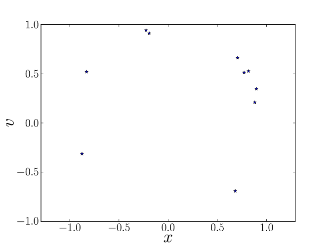
Figure 1: A sample of $N=10$ stars drawn from a one-dimensional toy galaxy with a simple harmonic oscillator potential $\Phi(x)=\frac{1}{2}\omega_{0}^{2}x^{2}$ in which $\omega_{0}=1$. The underlying DF of the model is a uniform distribution in amplitude $a$ between $a=0.9$ and $a=1$, where $a^{2}=x^{2}+v^{2}/\omega_{0}^{2}$.

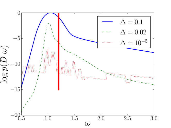
Figure 2: The likelihood $\mathop{\hbox{pr}}(D|\omega)$ for the sample of 10 stars shown in Figure 1 calculated using the standard maximum likelihood-based algorithm by adding nominal Gaussian error circles of standard deviation $\Delta$ around each observed $(x,v)$. The results for different choices of $\Delta$ have been offset for clarity. As $\Delta\to 0$ the models cannot distinguish one potential from another. For comparison, the heavy vertical red line indicates the estimate (3) of $\omega$ obtained by using the virial theorem.

Let us see how well such a scheme works when applied to our toy one-dimensional problem. Figure 1 shows a sample of $N=10$ stars drawn from a galaxy with $\omega_{0}=1$ and the annular top-hat DF

$$f(J)=\begin{cases}A,&\hbox{if $0.9<a(x,v)<1$,}\\ 0,&\hbox{otherwise},\end{cases}$$ (4)

where $A>0$ is an uninteresting normalisation constant and the amplitude $a(x,v)$ of an orbit passing through $(x,v)$ is defined to be

$$a^{2}(x,v)\equiv x^{2}+\frac{v^{2}}{\omega^{2}}=\frac{2\pi J}{\omega},$$ (5)

which for visualisation purposes is more convenient to use than the action $J$ when labelling orbits on the phase plane. To illustrate the effects of observational uncertainties, we assign nominal Gaussian errors of standard deviation $\Delta$ to each $(x^{\star}_{n},v^{\star}_{n})$ and consider the effects of shrinking $\Delta$ towards zero.

We use the four-step modelling procedure above to assign a likelihood $\mathop{\hbox{pr}}(D|\omega)$ to each of a range of trial values of $\omega$. The DF is modelled by a set of abutting annuli, with $f_{k}(x,v)=\hbox{constant}$ for amplitudes $a_{k}^{2}<x^{2}+v^{2}/\omega^{2}<a_{k+1}^{2}$, zero otherwise. There are $200$ such annuli, running from $a_{1}=0$ to $a_{201}=2$ with uniform spacing $a_{k+1}-a_{k}=0.01$. The contribution $P_{nk}$ that the $k^{\rm th}$ such annulus makes to the probability of observing the $n^{\rm th}$ star is simply the integral of $f_{k}(x,v)$ times a Gaussian of width $\Delta$ centred on $(x^{\star}_{n},v^{\star}_{n})$. Having calculated these $P_{nk}$, we use the expectation–maximisation algorithm to find the set of weights $w_{k}$ that maximise the likelihood subject to the constraint that $\sum_{k}w_{k}=1$

The resulting plot of maximum likelihood versus assumed $\omega$ for this dataset is shown on Figure 2. When $\Delta$ is large, this procedure produces a likelihood distribution $\mathop{\hbox{pr}}(D|\omega)$ that peaks close to the correct value of $\omega_{0}=1$. Perversely, however, the likelihood flattens as $\Delta$ shrinks: if the data become too good, the model is unable to distinguish one potential from another! It is easy to see why this is: given perfect knowledge of $(x^{\star}_{n},v^{\star}_{n})$ there is a unique orbit in (almost) any given potential that passes through this $(x^{\star}_{n},v^{\star}_{n})$ and no other; it is only when several stars lie along an orbit that one can say anything about the likelihood of the assumed potential. Therefore all potentials have the same likelihood.

2.3 Comments

What to do about this? One remedy is to consider only strongly parametrised forms for the DF or to take a non-parametric DF and impose some form of regularisation (e.g., Merritt, 1993), but this has the disadvantage of introducing hard-to-understand biases in $\mathop{\hbox{pr}}(D|\Phi)$. A related idea would be to somehow couple the resolution of the basis functions $f_{k}$ to some properties of the available sample $D$. Fundamentally, however, the problem with the maximum-likelihood procedure above is that it looks only at the distribution of orbits that produces the best possible match to the observed sample, with no regard for nearby orbit distributions that are only slightly less likely.

3 Modelling the distribution of DFs as a Dirichlet process mixture

Here is a more general restatement of the toy problem above. We have a galaxy with unknown potential $\Phi({\bf x})$ and unknown DF $f({\bf x},{\bf v})$. We are given a list of the phase-space locations $({\bf x}^{\star}_{n},{\bf v}^{\star}_{n})$ of $N$ stars drawn from the galaxy. We may assume that the galaxy is in a steady state and that the list of stars is a fair sample of the underlying DF. Our job is to constrain the potential from these data $D$. In particular, we seek the posterior probability distribution $\mathop{\hbox{pr}}(\Phi|D)$. By Bayes’ theorem $\mathop{\hbox{pr}}(\Phi|D)$ is proportional to $\mathop{\hbox{pr}}(D|\Phi)\mathop{\hbox{pr}}(\Phi)$, where $\mathop{\hbox{pr}}(\Phi)$ is our prior on $\Phi$.

As the galaxy is in a steady state, it is natural to express the DF in terms of action–angle coordinates $({\bf J},{\mathchoice{\hbox{{\gkvecten\char 18\relax}}}{\hbox{{\gkvecten\char 18\relax}}}{\hbox{{\gkvecseven\char 18\relax}}}{\hbox{{\gkvecseven\char 18\relax}}}})$ instead of $({\bf x},{\bf v})$: by the strong Jeans theorem, the DF is a function $f({\bf J})$ of the actions only (BT08). Let $d=1$, 2 or 3 be the number of dimensions in the system. If $d=3$ then we may take ${\bf J}=(J_{r},J_{\theta},J_{\phi})$ in which the radial action $J_{r}$ and the latitudinal action $J_{\theta}$ must be non-negative. The azimuthal action $J_{\phi}$ can take either sign. Similarly, for $d=2$ we have ${\bf J}=(J_{r},J_{\phi})$ in which $J_{r}\geq 0$, while for $d=1$ the single action $J\geq 0$. The likelihood $\mathop{\hbox{pr}}(D|\Phi)$ can be expressed in terms of the stars’ actions ${\bf J}^{\star}_{1}...{\bf J}^{\star}_{N}$ as

$$\begin{split}\mathop{\hbox{pr}}(D|\Phi,{\cal A})&=\int{\rm d}^{d}{\bf J}^{\star}_{1}{\rm d}^{d}{\mathchoice{\hbox{{\gkvecten\char 18\relax}}}{\hbox{{\gkvecten\char 18\relax}}}{\hbox{{\gkvecseven\char 18\relax}}}{\hbox{{\gkvecseven\char 18\relax}}}}^{\star}_{1}\mathop{\hbox{pr}}({\bf x}^{\star}_{1},{\bf v}^{\star}_{1}|{\bf J}_{1}^{\star},{\mathchoice{\hbox{{\gkvecten\char 18\relax}}}{\hbox{{\gkvecten\char 18\relax}}}{\hbox{{\gkvecseven\char 18\relax}}}{\hbox{{\gkvecseven\char 18\relax}}}}^{\star}_{1},\Phi)\cdots\\ &\int{\rm d}^{d}{\bf J}^{\star}_{N}{\rm d}^{d}{\mathchoice{\hbox{{\gkvecten\char 18\relax}}}{\hbox{{\gkvecten\char 18\relax}}}{\hbox{{\gkvecseven\char 18\relax}}}{\hbox{{\gkvecseven\char 18\relax}}}}^{\star}_{N}\mathop{\hbox{pr}}({\bf x}^{\star}_{N},{\bf v}^{\star}_{N}|{\bf J}_{N}^{\star},{\mathchoice{\hbox{{\gkvecten\char 18\relax}}}{\hbox{{\gkvecten\char 18\relax}}}{\hbox{{\gkvecseven\char 18\relax}}}{\hbox{{\gkvecseven\char 18\relax}}}}^{\star}_{N},\Phi)\,\cdot\,\mathop{\hbox{pr}}({\bf J}_{1}^{\star}\cdots{\bf J}_{N}^{\star}|{\cal A}),\end{split}$$ (6)

where ${\cal A}$ denotes some as-yet unstated assumptions (which will be summarised in §3.4 below) and each $\mathop{\hbox{pr}}({\bf x}^{\star}_{n},{\bf v}^{\star}_{n}|{\bf J}^{\star}_{n},{\mathchoice{\hbox{{\gkvecten\char 18\relax}}}{\hbox{{\gkvecten\char 18\relax}}}{\hbox{{\gkvecseven\char 18\relax}}}{\hbox{{\gkvecseven\char 18\relax}}}}^{\star}_{n},\Phi)$ is simply a Dirac delta that picks out the ${\bf J}^{\star}_{n}$ corresponding to $({\bf x}^{\star}_{n},{\bf v}^{\star}_{n})$ for the assumed $\Phi$. The only place that the potential enters into this problem is in the conversion from $({\bf x}^{\star}_{n},{\bf v}^{\star}_{n})$ to $({\bf J}^{\star}_{n},{\mathchoice{\hbox{{\gkvecten\char 18\relax}}}{\hbox{{\gkvecten\char 18\relax}}}{\hbox{{\gkvecseven\char 18\relax}}}{\hbox{{\gkvecseven\char 18\relax}}}}^{\star}_{n})$; when expressed in terms of the actions, the likelihood $\mathop{\hbox{pr}}({\bf J}^{\star}_{1}...{\bf J}^{\star}_{N}|{\cal A})$ is independent of $\Phi$.

The DF does not appear explicitly in the innocuous-looking expression $\mathop{\hbox{pr}}({\bf J}^{\star}_{1}...{\bf J}^{\star}_{N}|{\cal A})$ because it has been marginalised out: we have that

$$\mathop{\hbox{pr}}({\bf J}^{\star}_{1}...{\bf J}^{\star}_{N}|{\cal A})=\int\mathop{\hbox{pr}}({\bf J}^{\star}_{1}...{\bf J}^{\star}_{N}|f,{\cal A})\mathop{\hbox{pr}}({\rm d}f|{\cal A})$$ (7)

which involves summing the likelihood $\mathop{\hbox{pr}}({\bf J}^{\star}_{1}...{\bf J}^{\star}_{N}|f,{\cal A})$ over all DFs $f({\bf J})$ that satisfy the uniform-in-angle constraint imposed by Jeans’ theorem. There remains the choice of prior measure $\mathop{\hbox{pr}}({\rm d}f|{\cal A})$, which is a distribution over distributions. A standard way of choosing this, well known from the statistics and machine-learning communities, is to model the DF as being drawn from a Dirichlet process mixture: essentially, $f({\bf J})$ is expressed as a sum of an arbitrary number of blobs in action space, the blobs having some distribution of locations, sizes, shapes and probability masses. The marginal likelihood (7) is obtained by marginalising the parameters that describe the blobs. This basic idea is explained more precisely below, with further discussion postponed until Section 5.

In the following let $V$ be a large, but finite, volume of action space $(J_{\rm box})^{d}$ that includes all of the ${\bf J}_{n}^{\star}$ and let $H$ be a measure on this space. We take $H$ to be proportional to the canonical $(2\pi)^{d}{\rm d}^{d}{\bf J}$ phase-space volume, normalised so that $H(V)=1$.

3.1 Dirichlet distribution

Consider an arbitrary partition $P$ of action space $V$ into an arbitrary number $K$ of cells. Let $V_{k}$ be the subvolume enclosed by the $k^{\rm th}$ cell and let $\pi_{k}$ be the associated probability mass: that is, $\pi_{k}$ is an integral over the unknown DF within $V_{k}$. As the DF is unknown, we may treat ${\mathchoice{\hbox{{\gkvecten\char 25\relax}}}{\hbox{{\gkvecten\char 25\relax}}}{\hbox{{\gkvecseven\char 25\relax}}}{\hbox{{\gkvecseven\char 25\relax}}}}=(\pi_{1},...,\pi_{K})$ as a list of random variables. Clearly the $\pi_{k}$ must satisfy the conditions $\pi_{k}\geq 0$ and $\sum_{k=1}^{K}\pi_{k}=1$. For simplicity, let us assume that the $\pi_{k}$ are independent of one another. This is a strong assumption, whose consequences are discussed at the end of section 3.2 and further in section 5 below.

Recognising that the choice of partition $P$ is arbitrary yields an important constraint on the prior $\mathop{\hbox{pr}}({\mathchoice{\hbox{{\gkvecten\char 25\relax}}}{\hbox{{\gkvecten\char 25\relax}}}{\hbox{{\gkvecseven\char 25\relax}}}{\hbox{{\gkvecseven\char 25\relax}}}})$. Given any $P$, we may construct a new partition $P^{\prime}$ by merging, say, the first two cells of $P$ together, so that the volume of the first cell of $P^{\prime}$ is $V_{12}=V_{1}\cup V_{2}$, with associated probability mass $\pi_{12}=\pi_{1}+\pi_{2}$. Conversely, given $P^{\prime}$ we can construct $P$ by splitting one of the cells of $P^{\prime}$ into two. For consistency, the prior on $P^{\prime}$ should be related to the prior on $P$ through

$$\begin{split}\mathop{\hbox{pr}}(\pi_{12},\pi_{3},...,\pi_{K}|P^{\prime})&=\int{\rm d}\pi_{1}\int{\rm d}\pi_{2}\,\delta(\pi_{1}+\pi_{2}-\pi_{12})\times\\ &\quad\qquad\mathop{\hbox{pr}}(\pi_{1},\pi_{2},\pi_{3},...,\pi_{K}|P).\\ \end{split}$$ (8)

A particularly simple form for the prior that satisfies these conditions is the Dirichlet distribution, which has probability density function

$${\cal D}({\mathchoice{\hbox{{\gkvecten\char 25\relax}}}{\hbox{{\gkvecten\char 25\relax}}}{\hbox{{\gkvecseven\char 25\relax}}}{\hbox{{\gkvecseven\char 25\relax}}}}|{\mathchoice{\hbox{{\gkvecten\char 11\relax}}}{\hbox{{\gkvecten\char 11\relax}}}{\hbox{{\gkvecseven\char 11\relax}}}{\hbox{{\gkvecseven\char 11\relax}}}})\equiv\delta\left(1-\sum_{l=1}^{K}\pi_{l}\right)C({\mathchoice{\hbox{{\gkvecten\char 11\relax}}}{\hbox{{\gkvecten\char 11\relax}}}{\hbox{{\gkvecseven\char 11\relax}}}{\hbox{{\gkvecseven\char 11\relax}}}})\prod_{k=1}^{K}\pi_{k}^{-1+\alpha_{k}},$$ (9)

where the free parameters ${\mathchoice{\hbox{{\gkvecten\char 11\relax}}}{\hbox{{\gkvecten\char 11\relax}}}{\hbox{{\gkvecseven\char 11\relax}}}{\hbox{{\gkvecseven\char 11\relax}}}}=(\alpha_{1},...,\alpha_{K})$ satisfy $\alpha_{k}>0$, and the normalising constant

$$C({\mathchoice{\hbox{{\gkvecten\char 11\relax}}}{\hbox{{\gkvecten\char 11\relax}}}{\hbox{{\gkvecseven\char 11\relax}}}{\hbox{{\gkvecseven\char 11\relax}}}})\equiv\frac{\Gamma\left(\sum_{k=1}^{K}\alpha_{k}\right)}{\prod_{k=1}^{K}\Gamma(\alpha_{k})},$$ (10)

with $\Gamma(\alpha)$ the usual Gamma function. A convenient shorthand for (9) is

$$(\pi_{1},...,\pi_{K})\sim{\cal D}(\alpha_{1},...,\alpha_{K}),$$ (11)

the $\sim$ sign here meaning “is distributed as”. It is not hard to show that, if

$$(\pi_{1},\pi_{2},\ldots,\pi_{K})\sim{\cal D}(\alpha_{1},\alpha_{2},\alpha_{3},\ldots,\alpha_{K}),$$ (12)

then

$$(\pi_{12},\pi_{3},\ldots,\pi_{K})\sim{\cal D}(\alpha_{1}+\alpha_{2},\alpha_{3},\ldots,\alpha_{K}).$$ (13)

Therefore the prior (9) sastifies the consistency condition (8) as long as we choose the coefficients $\alpha_{k}$ proportional to the volume measure $H(V_{k})$ associated with each cell.

3.2 Dirichlet process

The consistency condition (8) means that we may restrict our attention in the following to priors defined on a large number $K$ of very small cells that all have the same volume and differ only their locations ${\bf J}_{k}$ in action space. As the cells have identical volumes, they must also have identical values of $\alpha_{k}$. So, let us take $\alpha_{k}=\alpha/K$ and consider the limit $K\to\infty$ (Neal, 2000; Rasmussen, 2000).

Any partition of $V$ into a finite number of nonempty, non-overlapping subvolumes, $(V_{1},...,V_{L})$, can be represented by grouping together these tiny, equal-volume cells; each of the $K$ cells will lie inside precisely one of the $V_{l}$. Let $F(V_{l})$ be the probability mass associated with $V_{l}$, so that $F(V_{l})=\sum_{V_{k}\in V_{l}}\pi_{k}$. Using the consistency property (8) of the Dirichlet distribution (9) together with the choice $\alpha(V_{l})=\alpha H(V_{l})$, it is obvious that for any such partition $(V_{1},...,V_{L})$ of $V$ we have that

$$(F(V_{1}),...,F(V_{L}))\sim{\cal D}(\alpha H(V_{1}),...,\alpha H(V_{L})).$$ (14)

This is the defining property of a Dirichlet process (Ferguson (1973); see also Teh (2010) for a brief, accessible introduction). A Dirichlet process has two parameters. One is the base measure $H$, which we take to be proportional to the canonical volume element $(2\pi)^{d}{\rm d}^{d}{\bf J}$. The other is the concentration parameter $\alpha$, which controls the clumpiness of the distribution: the expectation value of $F(V_{l})$ is just $H(V_{l})$ and the variance is $H(V_{l})(1-H(V_{l}))/(\alpha+1)$; as $\alpha$ increases the variance shrinks.

To understand more about the properties of draws from a Dirichlet process and the effect of $\alpha$, let us return to the picture of the limit of a large number $K\to\infty$ of equal-volume cells and suppose we draw $N$ stars from the distribution (9). Let $c_{i}\in\{1,...,K\}$ be the cell number of the $i^{\rm th}$ star. Clearly, $\mathop{\hbox{pr}}(c_{i}=c)=\pi_{c}$: the probability that the $i^{\rm th}$ draw picks cell $c$ is just $\pi_{c}$. Marginalising ${\mathchoice{\hbox{{\gkvecten\char 25\relax}}}{\hbox{{\gkvecten\char 25\relax}}}{\hbox{{\gkvecseven\char 25\relax}}}{\hbox{{\gkvecseven\char 25\relax}}}}=(\pi_{1},...,\pi_{K})$ with the prior (9), the probability of drawing star 1 from cell $c_{1}$, …, star $N$ from cell $c_{N}$ is

$$\begin{split}&\mathop{\hbox{pr}}(c_{1}...c_{N})\\ &=\frac{\Gamma(\alpha)}{\left[\Gamma\left(\frac{\alpha}{K}\right)\right]^{K}}\int{\rm d}{\mathchoice{\hbox{{\gkvecten\char 25\relax}}}{\hbox{{\gkvecten\char 25\relax}}}{\hbox{{\gkvecseven\char 25\relax}}}{\hbox{{\gkvecseven\char 25\relax}}}}\delta\left(1-\sum_{l=1}^{K}\pi_{l}\right)\,\pi_{c_{1}}\cdots\pi_{c_{N}}\pi_{1}^{-1+\alpha/K}\cdots\pi_{K}^{-1+\alpha/K}\\ &=\frac{\Gamma(\alpha)}{\left[\Gamma\left(\frac{\alpha}{K}\right)\right]^{K}\Gamma(N+\alpha)}\prod_{k=1}^{K}{\Gamma\left(n_{k}(N)+\frac{\alpha}{K}\right)},\end{split}$$ (15)

where $n_{k}(N)$ is the number of stars in cell $k$ for this draw of $N$ stars. Therefore the conditional probability

$$\mathop{\hbox{pr}}(c_{N}=c|c_{1},...,c_{N-1})=\frac{\mathop{\hbox{pr}}(c_{1}...c_{N})}{\mathop{\hbox{pr}}(c_{1}...c_{N-1})}=\frac{n_{k}(N)+\frac{\alpha}{K}}{N-1+\alpha}.$$ (16)

So, the first star is equally likely to come from any of the $K$ cells. In the limit $K\to\infty$ the second star has probability $1/(1+\alpha)$ of coming from the same cell as the first star. The remaining probability $\alpha/(1+\alpha)$ is spread equally among the unoccupied cells. More generally, star $N$ has probability $n/(N-1+\alpha)$ of coming from a cell that already holds $n$ stars. The probability that it does not come from a cell occupied by any of the previous $N-1$ stars is $\alpha/(N-1+\alpha)$. The same behaviour can be derived directly from the more abstract definition (14). When $N$ is large the expectation value of the number of non-empty cells tends to $\alpha\log(1+N/\alpha)$ (e.g., Antoniak, 1974; Teh, 2010).

This argument shows that if we use the $\pi_{k}$ to represent the DF directly the DF will be a series of isolated spikes: neighbouring parts of action space do not “know” about each other. Clearly then the marginal likelihood (7) would be independent of how the ${\bf J}_{n}^{\star}$ are distributed, unless two or more of them happen to overlap precisely. Therefore $\mathop{\hbox{pr}}(D|\Phi)$ would be flat, just as we found for the models in Figure 2. In fact, any prior that treats the $\pi_{k}$ as independent variables subject to the consistency condition (8) will produce spiky, discrete DFs (Kingman, 1992) and therefore will suffer from this problem.

3.3 Dirichlet process mixture of blobs

In order to give the prior on the DF some notion of continuity, let us smear out the probability mass $\pi_{k}$ associated with the $k^{\rm th}$ cell around the cell’s location ${\bf J}_{k}$ with density proportional to some function $\mathop{\hbox{Blob}}({\bf J}^{\star}|{\bf J}_{k},{\mathchoice{\hbox{{\gkvecten\char 3\relax}}}{\hbox{{\gkvecten\char 3\relax}}}{\hbox{{\gkvecseven\char 3\relax}}}{\hbox{{\gkvecseven\char 3\relax}}}}_{k})$, where ${\mathchoice{\hbox{{\gkvecten\char 3\relax}}}{\hbox{{\gkvecten\char 3\relax}}}{\hbox{{\gkvecseven\char 3\relax}}}{\hbox{{\gkvecseven\char 3\relax}}}}_{k}$ describes the size and shape of the blob. Then the DF becomes

$$f({\bf J})=\sum_{k=1}^{K}\pi_{k}\mathop{\hbox{Blob}}({\bf J}|{\bf J}_{k},{\mathchoice{\hbox{{\gkvecten\char 3\relax}}}{\hbox{{\gkvecten\char 3\relax}}}{\hbox{{\gkvecseven\char 3\relax}}}{\hbox{{\gkvecseven\char 3\relax}}}}_{k}),$$ (17)

with $\pi_{k}$ drawn from the Dirichlet distribution (9) with $\alpha_{k}=\alpha/K$. The parameters $\pi_{k}$, ${\bf J}_{k}$ and ${\mathchoice{\hbox{{\gkvecten\char 3\relax}}}{\hbox{{\gkvecten\char 3\relax}}}{\hbox{{\gkvecseven\char 3\relax}}}{\hbox{{\gkvecseven\char 3\relax}}}}_{k}$ of the blob associated with each cell are completely independent, save for the fact that $\sum_{k}\pi_{k}=1$. It is perhaps helpful to think of the DF (17) as representing the galaxy by a sum of its progenitor stellar clusters in phase space, the tidal debris from each cluster smeared out by two-body encounters and other relaxation effects, but we emphasise that the blobs are fundamentally purely formal devices used to introduce neighbouring parts of action space to one another.

In the absence of any constraints other than the location parameter ${\bf J}_{k}$ and the scale/shape parameter ${\mathchoice{\hbox{{\gkvecten\char 3\relax}}}{\hbox{{\gkvecten\char 3\relax}}}{\hbox{{\gkvecseven\char 3\relax}}}{\hbox{{\gkvecseven\char 3\relax}}}}_{k}$, a natural way of representing each blob would be by using a single Gaussian. Recall, however, that at least one of the components of ${\bf J}$ is constrained to be non-negative and yet we want $\pi_{k}$ to be the total probability mass of the blob. This means that the function $\mathop{\hbox{Blob}}({\bf J}|{\bf J}_{k},{\mathchoice{\hbox{{\gkvecten\char 3\relax}}}{\hbox{{\gkvecten\char 3\relax}}}{\hbox{{\gkvecseven\char 3\relax}}}{\hbox{{\gkvecseven\char 3\relax}}}}_{k})$ must have unit mass when integrated over the physically allowed region of action space. To ensure this, we take

$$\mathop{\hbox{Blob}}({\bf J}|{\bf J}_{k},{\mathchoice{\hbox{{\gkvecten\char 3\relax}}}{\hbox{{\gkvecten\char 3\relax}}}{\hbox{{\gkvecseven\char 3\relax}}}{\hbox{{\gkvecseven\char 3\relax}}}}_{k})=\sum_{m=1}^{M}{\cal N}({\bf J}|R_{m}{\bf J}_{k},{\mathchoice{\hbox{{\gkvecten\char 3\relax}}}{\hbox{{\gkvecten\char 3\relax}}}{\hbox{{\gkvecseven\char 3\relax}}}{\hbox{{\gkvecseven\char 3\relax}}}}_{k}^{-1}),$$ (18)

in which ${\cal N}$ is the usual normal distribution,

$${\cal N}({\bf x}|\bar{\bf x},{\mathchoice{\hbox{{\gkvecten\char 3\relax}}}{\hbox{{\gkvecten\char 3\relax}}}{\hbox{{\gkvecseven\char 3\relax}}}{\hbox{{\gkvecseven\char 3\relax}}}}^{-1})\equiv\frac{|{\mathchoice{\hbox{{\gkvecten\char 3\relax}}}{\hbox{{\gkvecten\char 3\relax}}}{\hbox{{\gkvecseven\char 3\relax}}}{\hbox{{\gkvecseven\char 3\relax}}}}|^{1/2}}{(2\pi)^{d/2}}\exp\left[-\frac{1}{2}({\bf x}-\bar{\bf x})^{T}{\mathchoice{\hbox{{\gkvecten\char 3\relax}}}{\hbox{{\gkvecten\char 3\relax}}}{\hbox{{\gkvecseven\char 3\relax}}}{\hbox{{\gkvecseven\char 3\relax}}}}({\bf x}-\bar{\bf x})\right],$$ (19)

where $|{\mathchoice{\hbox{{\gkvecten\char 3\relax}}}{\hbox{{\gkvecten\char 3\relax}}}{\hbox{{\gkvecseven\char 3\relax}}}{\hbox{{\gkvecseven\char 3\relax}}}}|$ is the determinant of the precision (i.e., inverse covariance) matrix Λ, and $R_{1},...,R_{M}$ are reflection operators that produce mirror images of the Gaussian at ${\bf J}={\bf J}_{k}$. For the case $d=3$ in which ${\bf J}=(J_{r},J_{\theta},J_{\phi})$ there are $M=4$ such operators:

$$\begin{split}R_{1}&=\mathop{\hbox{diag}}(+1,+1,+1),\\ R_{2}&=\mathop{\hbox{diag}}(-1,+1,+1),\\ R_{3}&=\mathop{\hbox{diag}}(+1,-1,+1),\\ R_{4}&=\mathop{\hbox{diag}}(-1,-1,+1).\end{split}$$ (20)

These reflect the original Gaussian centred on ${\bf J}={\bf J}_{k}$ about the $J_{r}=0$ and the $J_{\theta}=0$ axes so that the total mass of the blob in the physically allowed $J_{r}\geq 0$, $J_{\theta}\geq 0$ subvolume is equal to one. Similarly, for the $d=2$ case of ${\bf J}=(J_{r},J_{\phi})$ the necessary reflections are $R_{1}=\mathop{\hbox{diag}}(1,1)$, $R_{2}=\mathop{\hbox{diag}}(-1,1)$ and for $d=1$ they are simply $R_{1}=+1$, $R_{2}=-1$. Note that, although the first argument ${\bf J}$ of the function $\mathop{\hbox{Blob}}({\bf J}|{\bf J}_{k},{\mathchoice{\hbox{{\gkvecten\char 3\relax}}}{\hbox{{\gkvecten\char 3\relax}}}{\hbox{{\gkvecseven\char 3\relax}}}{\hbox{{\gkvecseven\char 3\relax}}}}_{k})$ has restrictions on the signs of some of its components, we do not need to impose any such restrictions on the second argument, ${\bf J}_{k}$. Therefore we allow the components of ${\bf J}_{k}$ to take either sign, so that, in the three-dimensional case, any of the four choices ${\bf J}_{k}=(\pm J_{r},\pm J_{\theta},J_{\phi})$ refer to the same blob.

In this scheme each cell has a characteristic width

$$\Delta J=2J_{\rm box}K^{-1/d}$$ (21)

that shrinks as $K\to\infty$. A priori, each star has probability

$$\mathop{\hbox{pr}}({\bf J}_{k}|\hbox{discrete})=1/K,$$ (22)

of belonging to the blob associated with cell $k$. In this point of view the blobs are treated as being “pinned” to the cell locations. In the continuum limit $K\to\infty$ we can forget about these underlying cells and use $\pi_{k}$ and ${\bf J}_{k}$ to refer directly to the probability mass and location of the $k^{\rm th}$ blob, the former having prior (14) and the latter

$$\mathop{\hbox{pr}}({\bf J}_{k}|\hbox{continuous})=\begin{cases}1/(2J_{\rm box})^{d},&\hbox{if all components $|J_{k,i}|<J_{\rm box}$},\\ 0,&\hbox{otherwise},\end{cases}$$ (23)

so that $\mathop{\hbox{pr}}({\bf J}_{k}|\hbox{continuous})(\Delta J)^{d}=\mathop{\hbox{pr}}({\bf J}_{k}|\hbox{discrete})$. Both ways of thinking about ${\bf J}_{k}$ are useful when deriving expressions for the marginal likelihood (Appendices B and C).

For the prior $\mathop{\hbox{pr}}({\mathchoice{\hbox{{\gkvecten\char 3\relax}}}{\hbox{{\gkvecten\char 3\relax}}}{\hbox{{\gkvecseven\char 3\relax}}}{\hbox{{\gkvecseven\char 3\relax}}}}_{k})$ on the precision matrix ${\mathchoice{\hbox{{\gkvecten\char 3\relax}}}{\hbox{{\gkvecten\char 3\relax}}}{\hbox{{\gkvecseven\char 3\relax}}}{\hbox{{\gkvecseven\char 3\relax}}}}_{k}$ we adopt the uninformative (e.g., Press, 2012) distribution

$$\begin{split}\mathop{\hbox{pr}}({\mathchoice{\hbox{{\gkvecten\char 3\relax}}}{\hbox{{\gkvecten\char 3\relax}}}{\hbox{{\gkvecseven\char 3\relax}}}{\hbox{{\gkvecseven\char 3\relax}}}}_{k})&=B_{0}|{\mathchoice{\hbox{{\gkvecten\char 3\relax}}}{\hbox{{\gkvecten\char 3\relax}}}{\hbox{{\gkvecseven\char 3\relax}}}{\hbox{{\gkvecseven\char 3\relax}}}}_{k}|^{-\frac{1}{2}(d+1)},\end{split}$$ (24)

but with a restriction on the range of allowed ${\mathchoice{\hbox{{\gkvecten\char 3\relax}}}{\hbox{{\gkvecten\char 3\relax}}}{\hbox{{\gkvecseven\char 3\relax}}}{\hbox{{\gkvecseven\char 3\relax}}}}_{k}$ to those that produce blobs that are larger than the cell size $\Delta J$ but smaller than $J_{\rm box}$. Appendix A gives the details of how we impose this restriction and calculate the dimensionless normalisation constant $B_{0}$.

Given a distribution of stars with actions ${\bf J}^{\star}_{1}$,…,${\bf J}^{\star}_{N}$, the likelihood is then

$$\begin{split}\mathop{\hbox{pr}}({\bf J}^{\star}_{1}...{\bf J}^{\star}_{N}|{\mathchoice{\hbox{{\gkvecten\char 25\relax}}}{\hbox{{\gkvecten\char 25\relax}}}{\hbox{{\gkvecseven\char 25\relax}}}{\hbox{{\gkvecseven\char 25\relax}}}},\{{\bf J},{\mathchoice{\hbox{{\gkvecten\char 3\relax}}}{\hbox{{\gkvecten\char 3\relax}}}{\hbox{{\gkvecseven\char 3\relax}}}{\hbox{{\gkvecseven\char 3\relax}}}}\})&=\prod_{n=1}^{N}\sum_{k=1}^{K}\pi_{k}\mathop{\hbox{Blob}}({\bf J}^{\star}_{n}|{\bf J}_{k},{\mathchoice{\hbox{{\gkvecten\char 3\relax}}}{\hbox{{\gkvecten\char 3\relax}}}{\hbox{{\gkvecseven\char 3\relax}}}{\hbox{{\gkvecseven\char 3\relax}}}}_{k}).\\ \end{split}$$ (25)

This awkward product of sums can be rewritten as an easier-to-handle sum of products,

$$\begin{split}\prod_{n=1}^{N}\sum_{k=1}^{K}\pi_{k}\mathop{\hbox{Blob}}({\bf J}^{\star}_{n}|{\bf J}_{k},{\mathchoice{\hbox{{\gkvecten\char 3\relax}}}{\hbox{{\gkvecten\char 3\relax}}}{\hbox{{\gkvecseven\char 3\relax}}}{\hbox{{\gkvecseven\char 3\relax}}}}_{k})=\sum_{{\bf Z}}\prod_{n=1}^{N}\prod_{k=1}^{K}\left[\pi_{k}\mathop{\hbox{Blob}}({\bf J}^{\star}_{n}|{\bf J}_{k},{\mathchoice{\hbox{{\gkvecten\char 3\relax}}}{\hbox{{\gkvecten\char 3\relax}}}{\hbox{{\gkvecseven\char 3\relax}}}{\hbox{{\gkvecseven\char 3\relax}}}}_{k})\right]^{z_{nk}}\end{split}$$ (26)

by introducing a set of binary variables ${\bf Z}=\{z_{nk}\}$ that indicate which of the $K$ blobs in equation (25) each of the $N$ stars comes from: $z_{nk}=1$ if star $n$ comes from the $k^{\rm th}$ blob and is zero otherwise; for each $n$ there is precisely one $k$ for which $z_{nk}=1$. Similarly, as the function $\mathop{\hbox{Blob}}({\bf J}^{\star}_{n}|{\bf J}_{k},{\mathchoice{\hbox{{\gkvecten\char 3\relax}}}{\hbox{{\gkvecten\char 3\relax}}}{\hbox{{\gkvecseven\char 3\relax}}}{\hbox{{\gkvecseven\char 3\relax}}}}_{k})$ is itself a sum of $M$ Gaussians, we can extend this idea and use $z_{nkm}$ to indicate which of the $K\times M$ Gaussians each star is drawn from. Then $z_{nk}=\sum_{m}z_{nkm}$. If we think of ${\bf Z}=\{z_{nkm}\}$ as a (latent) variable, then the likelihood becomes

$$\mathop{\hbox{pr}}({\bf J}^{\star}_{1}...{\bf J}^{\star}_{N},{\bf Z}|{\mathchoice{\hbox{{\gkvecten\char 25\relax}}}{\hbox{{\gkvecten\char 25\relax}}}{\hbox{{\gkvecseven\char 25\relax}}}{\hbox{{\gkvecseven\char 25\relax}}}},\{{\bf J},{\mathchoice{\hbox{{\gkvecten\char 3\relax}}}{\hbox{{\gkvecten\char 3\relax}}}{\hbox{{\gkvecseven\char 3\relax}}}{\hbox{{\gkvecseven\char 3\relax}}}}\})=\mathop{\hbox{pr}}({\bf J}^{\star}_{1}...{\bf J}^{\star}_{N}|{\bf Z},\{{\bf J},{\mathchoice{\hbox{{\gkvecten\char 3\relax}}}{\hbox{{\gkvecten\char 3\relax}}}{\hbox{{\gkvecseven\char 3\relax}}}{\hbox{{\gkvecseven\char 3\relax}}}}\})\mathop{\hbox{pr}}({\bf Z}|{\mathchoice{\hbox{{\gkvecten\char 25\relax}}}{\hbox{{\gkvecten\char 25\relax}}}{\hbox{{\gkvecseven\char 25\relax}}}{\hbox{{\gkvecseven\char 25\relax}}}}),$$ (27)

in which

$$\begin{split}\mathop{\hbox{pr}}({\bf J}^{\star}_{1}...{\bf J}^{\star}_{N}|{\bf Z},\{{\bf J},{\mathchoice{\hbox{{\gkvecten\char 3\relax}}}{\hbox{{\gkvecten\char 3\relax}}}{\hbox{{\gkvecseven\char 3\relax}}}{\hbox{{\gkvecseven\char 3\relax}}}}\})&=\prod_{n=1}^{N}\prod_{k=1}^{K}\left[\mathop{\hbox{Blob}}({\bf J}^{\star}_{n}|{\bf J}_{k},{\mathchoice{\hbox{{\gkvecten\char 3\relax}}}{\hbox{{\gkvecten\char 3\relax}}}{\hbox{{\gkvecseven\char 3\relax}}}{\hbox{{\gkvecseven\char 3\relax}}}}_{k})\right]^{z_{nk}}\\ &=\prod_{n=1}^{N}\prod_{k=1}^{K}\prod_{m=1}^{M}\left[{\cal N}({\bf J}^{\star}_{n}|R_{m}{\bf J}_{k},{\mathchoice{\hbox{{\gkvecten\char 3\relax}}}{\hbox{{\gkvecten\char 3\relax}}}{\hbox{{\gkvecseven\char 3\relax}}}{\hbox{{\gkvecseven\char 3\relax}}}}_{k}^{-1})\right]^{z_{nkm}}\end{split}$$ (28)

and

$$\mathop{\hbox{pr}}({\bf Z}|{\mathchoice{\hbox{{\gkvecten\char 25\relax}}}{\hbox{{\gkvecten\char 25\relax}}}{\hbox{{\gkvecseven\char 25\relax}}}{\hbox{{\gkvecseven\char 25\relax}}}})=\prod_{n=1}^{N}\prod_{k=1}^{K}\pi_{k}^{z_{nk}}=\prod_{n=1}^{N}\prod_{k=1}^{K}\prod_{m=1}^{M}\pi_{k}^{z_{nkm}}.$$ (29)

The true likelihood (25) is obtained by summing (27) over all possible assignments ${\bf Z}$ of stars to blobs (or Gaussians).

Combining this likelihood with the priors on $(\pi,\{{\bf J},{\mathchoice{\hbox{{\gkvecten\char 3\relax}}}{\hbox{{\gkvecten\char 3\relax}}}{\hbox{{\gkvecseven\char 3\relax}}}{\hbox{{\gkvecseven\char 3\relax}}}}\})$ introduced above yields the “probability of everything”,

$$\begin{split}&\mathop{\hbox{pr}}({\bf J}^{\star}_{1}...{\bf J}^{\star}_{N},{\bf Z},{\mathchoice{\hbox{{\gkvecten\char 25\relax}}}{\hbox{{\gkvecten\char 25\relax}}}{\hbox{{\gkvecseven\char 25\relax}}}{\hbox{{\gkvecseven\char 25\relax}}}},\{{\bf J},{\mathchoice{\hbox{{\gkvecten\char 3\relax}}}{\hbox{{\gkvecten\char 3\relax}}}{\hbox{{\gkvecseven\char 3\relax}}}{\hbox{{\gkvecseven\char 3\relax}}}}\})\\ &\qquad\qquad=\mathop{\hbox{pr}}({\bf J}^{\star}_{1}...{\bf J}^{\star}_{N},{\bf Z}|{\mathchoice{\hbox{{\gkvecten\char 25\relax}}}{\hbox{{\gkvecten\char 25\relax}}}{\hbox{{\gkvecseven\char 25\relax}}}{\hbox{{\gkvecseven\char 25\relax}}}},\{{\bf J},{\mathchoice{\hbox{{\gkvecten\char 3\relax}}}{\hbox{{\gkvecten\char 3\relax}}}{\hbox{{\gkvecseven\char 3\relax}}}{\hbox{{\gkvecseven\char 3\relax}}}}\})\mathop{\hbox{pr}}({\mathchoice{\hbox{{\gkvecten\char 25\relax}}}{\hbox{{\gkvecten\char 25\relax}}}{\hbox{{\gkvecseven\char 25\relax}}}{\hbox{{\gkvecseven\char 25\relax}}}})\mathop{\hbox{pr}}(\{{\bf J},{\mathchoice{\hbox{{\gkvecten\char 3\relax}}}{\hbox{{\gkvecten\char 3\relax}}}{\hbox{{\gkvecseven\char 3\relax}}}{\hbox{{\gkvecseven\char 3\relax}}}}\}).\end{split}$$ (30)

Since the DF is completely described by the parameters $({\mathchoice{\hbox{{\gkvecten\char 25\relax}}}{\hbox{{\gkvecten\char 25\relax}}}{\hbox{{\gkvecseven\char 25\relax}}}{\hbox{{\gkvecseven\char 25\relax}}}},\{{\bf J},{\mathchoice{\hbox{{\gkvecten\char 3\relax}}}{\hbox{{\gkvecten\char 3\relax}}}{\hbox{{\gkvecseven\char 3\relax}}}{\hbox{{\gkvecseven\char 3\relax}}}}\})$, we may obtain the marginal likelihood (7) from (30) by considering all possible assigments ${\bf Z}$ of stars to blobs, marginalising the blob parameters $({\mathchoice{\hbox{{\gkvecten\char 25\relax}}}{\hbox{{\gkvecten\char 25\relax}}}{\hbox{{\gkvecseven\char 25\relax}}}{\hbox{{\gkvecseven\char 25\relax}}}},\{{\bf J},{\mathchoice{\hbox{{\gkvecten\char 3\relax}}}{\hbox{{\gkvecten\char 3\relax}}}{\hbox{{\gkvecseven\char 3\relax}}}{\hbox{{\gkvecseven\char 3\relax}}}}\})$ for each choice of ${\bf Z}$, and summing the results:

$$\begin{split}&\mathop{\hbox{pr}}({\bf J}^{\star}_{1}...{\bf J}^{\star}_{N}|{\cal A})\\ &\qquad=\sum_{\bf Z}\int{\rm d}{\mathchoice{\hbox{{\gkvecten\char 25\relax}}}{\hbox{{\gkvecten\char 25\relax}}}{\hbox{{\gkvecseven\char 25\relax}}}{\hbox{{\gkvecseven\char 25\relax}}}}\int{\rm d}{\bf J}_{1...K}\int{\rm d}{\mathchoice{\hbox{{\gkvecten\char 3\relax}}}{\hbox{{\gkvecten\char 3\relax}}}{\hbox{{\gkvecseven\char 3\relax}}}{\hbox{{\gkvecseven\char 3\relax}}}}_{1...K}\,\mathop{\hbox{pr}}({\bf J}^{\star}_{1}...{\bf J}^{\star}_{N},{\bf Z},{\mathchoice{\hbox{{\gkvecten\char 25\relax}}}{\hbox{{\gkvecten\char 25\relax}}}{\hbox{{\gkvecseven\char 25\relax}}}{\hbox{{\gkvecseven\char 25\relax}}}},\{{\bf J},{\mathchoice{\hbox{{\gkvecten\char 3\relax}}}{\hbox{{\gkvecten\char 3\relax}}}{\hbox{{\gkvecseven\char 3\relax}}}{\hbox{{\gkvecseven\char 3\relax}}}}\}).\end{split}$$ (31)

3.4 Summary of probability distributions

The following lists the probability distributions introduced above and summarises the assumptions ${\cal A}$ made to calculate the marginal likelihood $\mathop{\hbox{pr}}({\bf J}^{\star}_{1}...{\bf J}^{\star}_{N}|{\cal A})$ of equation (7). The fundamental assumption is that the DF is uniform in angle and can be described by a sum of blobs (17) in action space. Then from equation (31) the marginal likelihood $\mathop{\hbox{pr}}({\bf J}^{\star}_{1}...{\bf J}^{\star}_{N}|{\cal A})$ is obtained by marginalising the “probability of everything”

$$\begin{split}\mathop{\hbox{pr}}({\bf J}^{\star}_{1}...{\bf J}^{\star}_{N},{\bf Z},{\mathchoice{\hbox{{\gkvecten\char 25\relax}}}{\hbox{{\gkvecten\char 25\relax}}}{\hbox{{\gkvecseven\char 25\relax}}}{\hbox{{\gkvecseven\char 25\relax}}}},\{{\bf J},{\mathchoice{\hbox{{\gkvecten\char 3\relax}}}{\hbox{{\gkvecten\char 3\relax}}}{\hbox{{\gkvecseven\char 3\relax}}}{\hbox{{\gkvecseven\char 3\relax}}}}\})&=\mathop{\hbox{pr}}({\bf J}^{\star}_{1}...{\bf J}^{\star}_{N}|{\bf Z},\{{\bf J},{\mathchoice{\hbox{{\gkvecten\char 3\relax}}}{\hbox{{\gkvecten\char 3\relax}}}{\hbox{{\gkvecseven\char 3\relax}}}{\hbox{{\gkvecseven\char 3\relax}}}}\})\mathop{\hbox{pr}}({\bf Z}|{\mathchoice{\hbox{{\gkvecten\char 25\relax}}}{\hbox{{\gkvecten\char 25\relax}}}{\hbox{{\gkvecseven\char 25\relax}}}{\hbox{{\gkvecseven\char 25\relax}}}})\\ &\qquad\times\mathop{\hbox{pr}}({\mathchoice{\hbox{{\gkvecten\char 25\relax}}}{\hbox{{\gkvecten\char 25\relax}}}{\hbox{{\gkvecseven\char 25\relax}}}{\hbox{{\gkvecseven\char 25\relax}}}})\mathop{\hbox{pr}}(\{{\bf J},{\mathchoice{\hbox{{\gkvecten\char 3\relax}}}{\hbox{{\gkvecten\char 3\relax}}}{\hbox{{\gkvecseven\char 3\relax}}}{\hbox{{\gkvecseven\char 3\relax}}}}\}),\end{split}$$ (32)

over the hidden variables ${\bf Z}$ and the model parameters $({\mathchoice{\hbox{{\gkvecten\char 25\relax}}}{\hbox{{\gkvecten\char 25\relax}}}{\hbox{{\gkvecseven\char 25\relax}}}{\hbox{{\gkvecseven\char 25\relax}}}},({\bf J}_{1},{\mathchoice{\hbox{{\gkvecten\char 3\relax}}}{\hbox{{\gkvecten\char 3\relax}}}{\hbox{{\gkvecseven\char 3\relax}}}{\hbox{{\gkvecseven\char 3\relax}}}}_{1}),...,({\bf J}_{K},{\mathchoice{\hbox{{\gkvecten\char 3\relax}}}{\hbox{{\gkvecten\char 3\relax}}}{\hbox{{\gkvecseven\char 3\relax}}}{\hbox{{\gkvecseven\char 3\relax}}}}_{K}))$ in the limit $K\to\infty$. The likelihood on the right-hand side of (32) is has two factors. One is a product of Gaussians,

$$\mathop{\hbox{pr}}({\bf J}^{\star}_{1}...{\bf J}^{\star}_{N}|{\bf Z},\{{\bf J},{\mathchoice{\hbox{{\gkvecten\char 3\relax}}}{\hbox{{\gkvecten\char 3\relax}}}{\hbox{{\gkvecseven\char 3\relax}}}{\hbox{{\gkvecseven\char 3\relax}}}}\}) =\prod_{n=1}^{N}\prod_{k=1}^{K}\prod_{m=1}^{M}\left[{\cal N}({\bf J}^{\star}_{n}|R_{m}{\bf J}_{k},{\mathchoice{\hbox{{\gkvecten\char 3\relax}}}{\hbox{{\gkvecten\char 3\relax}}}{\hbox{{\gkvecseven\char 3\relax}}}{\hbox{{\gkvecseven\char 3\relax}}}}_{k}^{-1})\right]^{z_{nkm}},$$ (33)

where the reflection operators $R_{m}$ are given by (20). The other is the multinomial

$$\mathop{\hbox{pr}}({\bf Z}|{\mathchoice{\hbox{{\gkvecten\char 25\relax}}}{\hbox{{\gkvecten\char 25\relax}}}{\hbox{{\gkvecseven\char 25\relax}}}{\hbox{{\gkvecseven\char 25\relax}}}})=\prod_{n=1}^{N}\prod_{k=1}^{K}\prod_{m=1}^{M}\pi_{k}^{z_{nkm}}.$$ (34)

The priors on the model parameters are

$$\mathop{\hbox{pr}}({\mathchoice{\hbox{{\gkvecten\char 25\relax}}}{\hbox{{\gkvecten\char 25\relax}}}{\hbox{{\gkvecseven\char 25\relax}}}{\hbox{{\gkvecseven\char 25\relax}}}}) ={\cal D}({\mathchoice{\hbox{{\gkvecten\char 25\relax}}}{\hbox{{\gkvecten\char 25\relax}}}{\hbox{{\gkvecseven\char 25\relax}}}{\hbox{{\gkvecseven\char 25\relax}}}}|{\mathchoice{\hbox{{\gkvecten\char 11\relax}}}{\hbox{{\gkvecten\char 11\relax}}}{\hbox{{\gkvecseven\char 11\relax}}}{\hbox{{\gkvecseven\char 11\relax}}}}_{0}),$$ (35)

$$\mathop{\hbox{pr}}(\{{\bf J},{\mathchoice{\hbox{{\gkvecten\char 3\relax}}}{\hbox{{\gkvecten\char 3\relax}}}{\hbox{{\gkvecseven\char 3\relax}}}{\hbox{{\gkvecseven\char 3\relax}}}}\}) =\prod_{k=1}^{K}\mathop{\hbox{pr}}({\bf J}_{k})\mathop{\hbox{pr}}({\mathchoice{\hbox{{\gkvecten\char 3\relax}}}{\hbox{{\gkvecten\char 3\relax}}}{\hbox{{\gkvecseven\char 3\relax}}}{\hbox{{\gkvecseven\char 3\relax}}}}_{k}),$$ (36)

$$\mathop{\hbox{pr}}({\bf J}_{k}) =\begin{cases}(2J_{\rm box})^{-d},&\hbox{if all components $|J_{k,i}|<J_{\rm box}$},\\ 0,&\hbox{otherwise},\end{cases}$$ (37)

$$\mathop{\hbox{pr}}({\mathchoice{\hbox{{\gkvecten\char 3\relax}}}{\hbox{{\gkvecten\char 3\relax}}}{\hbox{{\gkvecseven\char 3\relax}}}{\hbox{{\gkvecseven\char 3\relax}}}}_{k}) =B_{0}|{\mathchoice{\hbox{{\gkvecten\char 3\relax}}}{\hbox{{\gkvecten\char 3\relax}}}{\hbox{{\gkvecseven\char 3\relax}}}{\hbox{{\gkvecseven\char 3\relax}}}}_{k}|^{-\frac{1}{2}(d+1)},$$ (38)

with ${\mathchoice{\hbox{{\gkvecten\char 11\relax}}}{\hbox{{\gkvecten\char 11\relax}}}{\hbox{{\gkvecseven\char 11\relax}}}{\hbox{{\gkvecseven\char 11\relax}}}}_{0}=\textstyle\left(\frac{\alpha}{K},...,\frac{\alpha}{K}\right)$. The variables $\alpha$, $J_{\rm box}$ and $B_{0}$ are (degenerate) hyperparameters: a brief inspection of equations (32) to (38) shows that the model behaviour is controlled by the single hyperparameter

$$\alpha^{\prime}=\frac{\alpha B_{0}}{(2J_{\rm box})^{d}},$$ (39)

which has dimensions of $(\hbox{action-space volume})^{-1}$. Following the discussion in Section 3.2, the larger the value of $\alpha^{\prime}$ the larger the prior weight given to clumpy DFs that are composed of many blobs.

The model defined by equations (32)–(38) is a straightforward variant of the “infinite mixture of Gaussians” problem that is well known in the statistics and machine learning communities (e.g., Rasmussen, 2000). The only differences are that we have introduced the reflection matrices $R_{m}$ and, forsaking some computational convenience, have imposed explicitly noninformative priors on ${\bf J}_{k}$ and ${\mathchoice{\hbox{{\gkvecten\char 3\relax}}}{\hbox{{\gkvecten\char 3\relax}}}{\hbox{{\gkvecseven\char 3\relax}}}{\hbox{{\gkvecseven\char 3\relax}}}}_{k}$.

3.5 Comparison with the maximum-likelihood orbit-superposition (“extended Schwarzschild”) method

The maximum-likelihood orbit-superposition method (§2.2) can be viewed as a special case of the modelling procedure above in which one chooses a fixed set of blob parameters (${\bf J}_{k},{\mathchoice{\hbox{{\gkvecten\char 3\relax}}}{\hbox{{\gkvecten\char 3\relax}}}{\hbox{{\gkvecseven\char 3\relax}}}{\hbox{{\gkvecseven\char 3\relax}}}}_{k})$: the locations ${\bf J}_{k}$ are set by the choice of orbit library and the precisions are taken to be ${\mathchoice{\hbox{{\gkvecten\char 3\relax}}}{\hbox{{\gkvecten\char 3\relax}}}{\hbox{{\gkvecseven\char 3\relax}}}{\hbox{{\gkvecseven\char 3\relax}}}}_{k}=\frac{1}{\epsilon}I$, where $I$ is the identity matrix and $\epsilon\to 0$, so that each blob contracts to a single orbit. The only free parameters are then the “orbit weights” ß, the most likely set of which is taken to be indicative of all DFs in that potential. Section 2.2 lists a step-by-step procedure for applying the maximum-likelihood procedure in practice. For comparison, here are the corresponding steps in the Dirichlet process mixture method:

1. Instead of representing the DF as a weighted sum $f({\bf J})=\sum_{k}w_{k}f_{k}({\bf J})$ of fixed basis functions $f_{k}({\bf J})$, write it as a sum of an arbitrary number of blobs in action space (17), each blob having some unknown mass $\pi_{k}$, location ${\bf J}_{k}$ and shape ${\mathchoice{\hbox{{\gkvecten\char 3\relax}}}{\hbox{{\gkvecten\char 3\relax}}}{\hbox{{\gkvecseven\char 3\relax}}}{\hbox{{\gkvecseven\char 3\relax}}}}_{k}$.

2. For each datapoint $({\bf x}^{\star}_{n},{\bf v}^{\star}_{n})$, calculate the contribution to the likelihood,

   $$P_{nk} =\mathop{\hbox{pr}}(({\bf x}_{n}^{\star},{\bf v}_{n}^{\star})|{\bf J}_{k},{\mathchoice{\hbox{{\gkvecten\char 3\relax}}}{\hbox{{\gkvecten\char 3\relax}}}{\hbox{{\gkvecseven\char 3\relax}}}{\hbox{{\gkvecseven\char 3\relax}}}}_{k},\Phi)$$

   $$=\int\mathop{\hbox{pr}}({\bf x}_{n}^{\star},{\bf v}_{n}^{\star}|{\bf J}_{n}^{\star},\Phi)\mathop{\hbox{Blob}}({\bf J}^{\star}_{n}|{\bf J}_{k},{\mathchoice{\hbox{{\gkvecten\char 3\relax}}}{\hbox{{\gkvecten\char 3\relax}}}{\hbox{{\gkvecseven\char 3\relax}}}{\hbox{{\gkvecseven\char 3\relax}}}}_{k})\,{\rm d}^{d}{\bf J}^{\star}_{n},$$ (40)

   made by an arbitrary blob $({\bf J}_{k},{\mathchoice{\hbox{{\gkvecten\char 3\relax}}}{\hbox{{\gkvecten\char 3\relax}}}{\hbox{{\gkvecseven\char 3\relax}}}{\hbox{{\gkvecseven\char 3\relax}}}}_{k})$ in the assumed potential $\Phi$. For the special case of perfect, unbiased data focused on in this paper the $\mathop{\hbox{pr}}({\bf x}_{n}^{\star},{\bf v}_{n}^{\star}|{\bf J}_{n}^{\star},\Phi)$ factor in the integrand is a Dirac delta that picks out the actions ${\bf J}^{\star}_{n}$ of the orbit that passes through the point $({\bf x}^{\star}_{n},{\bf v}^{\star}_{n})$ and so $P_{nk}=\mathop{\hbox{Blob}}({\bf J}_{n}^{\star}|{\bf J}_{k},{\mathchoice{\hbox{{\gkvecten\char 3\relax}}}{\hbox{{\gkvecten\char 3\relax}}}{\hbox{{\gkvecseven\char 3\relax}}}{\hbox{{\gkvecseven\char 3\relax}}}}_{k})$. Unlike the corresponding step in the maximum-likelihood method, at this stage we cannot write down a numerical value for $P_{nk}$, because it depends on the nuisance parameters $({\bf J}_{k},{\mathchoice{\hbox{{\gkvecten\char 3\relax}}}{\hbox{{\gkvecten\char 3\relax}}}{\hbox{{\gkvecseven\char 3\relax}}}{\hbox{{\gkvecseven\char 3\relax}}}}_{k})$ which are marginalised in the next step.

3. Perform the marginalisation (31).

Note that the third step above combines the last two steps of the maximum-likelihood procedure of §2.2 into one.

4 Tests

In this section we present the results of calculating the marginal likelihood $\mathop{\hbox{pr}}(D|\Phi)$ given by equations (6) and (31) above for some simple test problems, starting with the one-dimensional simple harmonic oscillator of Section 2. We make use of two different schemes to compute the $\mathop{\hbox{pr}}({\bf J}^{\star}_{1}...{\bf J}^{\star}_{N}|{\cal A})$ given by equation (31):

1. an exact calculation obtained by reducing (31) to a sum over all possible partitions of the set of $N$ stars (equ. 80);

2. a variational lower bound (equ. 118) obtained by fitting a simple functional form to the integrand (32).

Although both schemes are simple to implement in practice, their derivations are quite involved and so we relegate the details to Appendices B and C respectively. Practical application of the exact calculation (i) is feasible only for small numbers of stars, $N<10$. In contrast, the approximate variational scheme (ii) is computationally inexpensive: Appendix C.2 provides step-by-step instructions on how to implement it.

4.1 One-dimensional simple harmonic oscillator

In the simple harmonic potential $\Phi(x)=\frac{1}{2}\omega^{2}x^{2}$ the action associated with a star that passes through the point $(x,v)$ is

$$J(x,v|\omega)=\frac{1}{2\pi}\oint\dot{x}\,{\rm d}x=\frac{\omega}{2\pi}\left(x^{2}+\frac{v^{2}}{\omega^{2}}\right).$$ (41)

For each of the sample $D$ of $N=10$ stars shown in Figure 1 changing the assumed $\omega$ changes the action $J_{n}^{\star}=J(x^{\star}_{n},v^{\star}_{n}|\omega)$. Figure 3 plots the marginal likelihood $\mathop{\hbox{pr}}(D|\omega)=\mathop{\hbox{pr}}(J_{1}^{\star},...,J_{N}^{\star})$ for a range of assumed values of $\omega$ using both the exact calculation of Appendix B and the variational estimate of Appendix C.

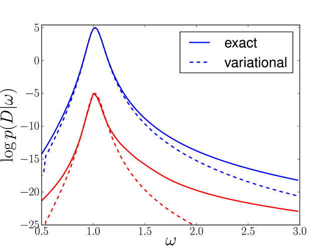
Figure 3: The marginalised likelihood $\mathop{\hbox{pr}}(D|\omega)$ for the sample of 10 stars shown in Figure 1 calculated using the exact method of Appendix B (solid curves) and the approximate variational method of Appendix C (dashed curves). The upper pair of curves are for concentration parameter $\alpha^{\prime}=10^{-3}$, the lower for $\alpha^{\prime}=10^{-1}$. The two pairs of curves have been offset vertically from one another for clarity. Compare to Figure 2.

This plot demonstrates two important points. The first, more practical, point is that the variational estimate (Appendix C) of the marginal likelihood agrees well with the exact calculation (Appendix B), especially for small values of the concentration parameter $\alpha^{\prime}$ (equ. 39). This is not surprising, as the variational estimate essentially approximates the integrand (32) by the contribution made by one or more well-chosen blobs, which will tend to be a good approximation for small $\alpha$. This is important, because even for only $N=10$ stars the exact calculation of $\mathop{\hbox{pr}}(D|\omega)$ takes a few seconds per $\omega$ on a standard PC, whereas the variational approximation is instantaneous.

The second point to note from Figure 3 is that, despite the relatively small number of stars, the marginal likelihood is sharply peaked about the correct value of $\omega=1$. The reason for this is that the Dirichlet process mixture used to model the DF favours DFs that are strongly peaked in action space. A quantitative explanation of this is given at the end of Appendix B, but to illustrate it we have constructed realisations of two different simple-harmonic oscillator models. The models have $\omega=1$ and $N=10$ stars drawn from a uniform distribution of stellar amplitudes $a$ between some $a_{\rm min}$ and $a_{\rm max}$. For one model we take the same narrow distribution of amplitudes, $(a_{\rm min},a_{\rm max})=(0.9,1.0)$, as used in Figures 1 to 3. For the other we use the broader $(a_{\rm min},a_{\rm max})=(0,1)$. For each realisation of each model Figure 4 compares the virial theorem estimate (3) of $\omega$ to the expectation value,

$$\omega_{\rm DPM}=\int\mathop{\hbox{pr}}(D|\omega)\mathop{\hbox{pr}}(\omega){\rm d}\omega,$$ (42)

obtained from the marginal likelihood $\mathop{\hbox{pr}}(D|\omega)$ (equ. 6) with an uninformative prior $\mathop{\hbox{pr}}(\omega)\propto 1/\omega$. It is evident from Figure 4 that the estimate (42) is much better than $\omega_{\rm VT}$ in the case of the model with the narrow distribution of amplitudes: $\omega_{\rm DPM}$ is always much closer the correct $\omega=1$ than $\omega_{\rm VT}$. The two estimates are comparable when the amplitude distribution is broad, however.

Figure 4: Comparison of the virial theorem estimate $\omega_{\rm VT}$ (equ. 3) to the marginal likelihood-based estimate $\omega_{\rm DPM}$ (equ. 42) for many realisations of a simple harmonic oscillator model having $N=10$ stars distributed uniformly in amplitude $a$ between $a_{\rm min}$ and $a_{\rm max}$. The panel on the left plots the comparison for $(a_{\rm min},a_{\rm max})=(0.9,1)$. The one on the right is for $(0,1)$.

Figure 5: Plots of $\log\mathop{\hbox{pr}}(D|\gamma,M)$ for the solar system problem of Section 4.2. The panel on the left shows the results of the exact calculation with (Appendix B) for concentration parameter $\alpha^{\prime}=10^{-4}\,\hbox{yr (AU)}^{-2}$. The middle panel shows the corresponding variational estimate (Appendix C). The panel on the right plots the exact result for $\alpha^{\prime}=10^{-2}\,\hbox{yr (AU)}^{-2}$.

4.2 Solar system

Bovy et al. (2010) have recently applied a broadly similar technique to constrain the force law in the solar system using only a snapshot of the positions and velocities of the eight major planets at a specific instance in time, albeit by assuming a parametric form for the DF from which the planets are drawn. We follow them by assuming that the potential in the solar system is of the form

$$\Phi(R)=-\frac{GM}{(\gamma+1)R_{0}}\left(\frac{R_{0}}{R}\right)^{\gamma+1},$$ (43)

so that a planet at radius $R$ feels a radial acceleration of magnitude

$$|\ddot{{\bf x}}|=-\frac{GM}{R_{0}^{2}}\left(\frac{R_{0}}{R}\right)^{\gamma}.$$ (44)

We set the reference radius $R_{0}=1\,\hbox{AU}$, leaving $\gamma$ and $M$ as free parameters. To illustrate the application of the method of Section 3 to a system with $d=2$ dimensions we ignore the motion out of the ecliptic plane. Then for an assumed $(\gamma,M)$, the two actions associated with an orbit that passes through the point $(x,y)$ in the ecliptic plane with velocity $(v_{x},v_{y})$ are

$$\begin{split}J_{R}({\bf x},{\bf v}|\Phi)&=\frac{1}{2\pi}\oint v_{R}\,{\rm d}R=\frac{1}{\pi}\int_{R_{-}}^{R_{+}}\left[2(E-\Phi)-\frac{L^{2}}{R^{2}}\right]^{1/2}\,{\rm d}R,\\ J_{\phi}({\bf x},{\bf v}|\Phi)&=\frac{1}{2\pi}\oint p_{\phi}\,{\rm d}\phi=L,\end{split}$$ (45)

where $L=xv_{y}-yv_{x}$ and $E=\frac{1}{2}{\bf v}^{2}+\Phi$ are the angular momentum and energy per unit mass respectively, and $R_{\pm}(E,L)$ are the corresponding apo- and peri-helion radii.

For each assumed $(\gamma,M)$ we calculate the actions $(J^{\star}_{R,n},J^{\star}_{\phi,n})$ associated with the positions $(x^{\star}_{n},y^{\star}_{n})$ and velocities $(v^{\star}_{x,n},v^{\star}_{y,n})$ of the eight major planets from the 1 April 2009 ephemeris in Table 1 of Bovy et al. (2010). Figure 5 shows the marginalised likelihood $\mathop{\hbox{pr}}(D|\gamma,M)=\mathop{\hbox{pr}}(\{(J^{\star}_{R,n},J^{\star}_{\phi,n})\}|{\cal A})$ calculated using both the exact method of Appendix B and the variational estimate of Appendix C. As in the case of the simple harmonic oscillator, the two methods agree well when the concentration parameter $\alpha^{\prime}$ is small. For larger $\alpha^{\prime}$ the exact $\mathop{\hbox{pr}}(D|\Phi)$ becomes implausibly clumpy, which cannot be reproduced by the variational estimate.

The resulting $\mathop{\hbox{pr}}(D|\gamma,M)$ is broadly similar to that obtained by Bovy et al. (2010, their Figure 6), who assumed various parametrised forms for the DF and used a Markov-Chain Monte Carlo method to explore the posterior distribution of their DF and potential parameters simultaneously. There are some differences: we see no evidence of the multimodal structure they found, and our posterior probability distribution is slightly tighter, with a stronger covariance between $\gamma$ and $M$. In common with them, we find that the model is only marginally consistent with the correct result of $(\gamma,M)=(2,M_{\odot})$. The marginal likelihood peaks at $(\gamma,M)\simeq(2.02,1.07\,M_{\odot})$: the model slightly overestimates the inward acceleration felt by the inner planets (including the earth), and slightly underestimates the accelerations further out. On the other hand, if we believe from Poisson’s equation that $\nabla^{2}\Phi\geq 0$ everywhere, then we must impose the prior constraint that $\gamma\leq 2$ and the resulting $\mathop{\hbox{pr}}(D|\gamma,M)$ is strongly peaked very close to the correct $M=M_{\odot}$ value.

4.3 A simple galaxy model

A more realistic example is provided by a catalogue of stars taken from a snapshot of an equilibrium galaxy model. The toy galaxy has a black hole of mass $M_{\bullet}$ embedded in a uniform, spherical distribution of dark matter with mass $M_{0}$ within a reference radius $r_{0}$. The potential is then

$$\Phi(r)=-\frac{GM_{\bullet}}{r}+\frac{GM_{0}}{2r_{0}^{3}}r^{2}.$$ (46)

Throughout the following we set the reference radius $r_{0}=1$. The stars in the galaxy are luminous test particles with a Hernquist (1990) number-density profile,

$$\rho(r)\propto\frac{1}{r(r_{\rm H}+r)^{3}}$$ (47)

and an isotropic internal velocity distribution. To create the simulated catalogue we use Eddington’s formula to find the distribution function $f(E)$ that produces the number-density profile (47) in the potential (46) and then generate mock observations by drawing $({\bf x}^{\star}_{n},{\bf v}^{\star}_{n})$ for $n=1,...,N=10^{4}$ stars from this DF. The model galaxy has $M_{\bullet}=M_{0}=1$, so that $r_{0}$ is approximately equal to the radius of the sphere of influence of the black hole. We choose $r_{\rm H}=r_{0}/(1+\sqrt{2})$, which places half of the stars inside $r_{0}$.

Figure 6: Plot of $\log\mathop{\hbox{pr}}(D|M_{\bullet},M_{\star})$ for the toy galaxy model of Section 4.3. Successive contour levels are spaced at $\Delta\log\mathop{\hbox{pr}}(D|M_{\bullet},M_{\star})=1$.

Having this catalogue of $10^{4}$ stars we use the variational method of Appendix C to approximate the marginal likelihood $\mathop{\hbox{pr}}(D|\Phi)$ for potentials $\Phi(r)$ of the form (46) with different assumed $(M_{\bullet},M_{\star})$. For each assumed $(M_{\bullet},M_{\star})$, the actions associated with an orbit that passes through the phase-space point $({\bf x},{\bf v})$ are

$$\begin{split}J_{r}({\bf x},{\bf v}|\Phi)&=\frac{1}{2\pi}\oint v_{r}\,{\rm d}r=\frac{1}{\pi}\int_{r_{-}}^{r_{+}}\left[2(E-\Phi)-\frac{L^{2}}{r^{2}}\right]^{1/2}\,{\rm d}r,\\ J_{\phi}({\bf x},{\bf v}|\Phi)&=\frac{1}{2\pi}\oint p_{\phi}\,{\rm d}\phi=L_{\phi},\\ J_{\theta}({\bf x},{\bf v}|\Phi)&=L-|L_{\phi}|,\end{split}$$ (48)

where $L=|{\bf x}\times{\bf v}|$, $L_{\phi}=xv_{y}-yv_{x}$ and $E=\frac{1}{2}{\bf v}^{2}+\Phi$ are the total angular momentum, its projection onto the $z$ axis and the energy per unit mass respectively, and $r_{\pm}(E,L)$ are the apo- and peri-centre radii. On an unremarkable standard PC the time taken to do the conversion from $\{({\bf x}^{\star}_{n},{\bf v}^{\star}_{n})\}$ to $\{{\bf J}_{n}^{\star}\}$ for the full sample of $N=10^{4}$ stars and construct the variational estimate was about 1 second for each $(M_{\bullet},M_{\star})$. The resulting marginalised likelihood (Figure 6) peaks very close to the correct $(M_{\bullet},M_{\star})=(1,1)$ parameters from which the stars were drawn.

5 Discussion

5.1 The choice of prior

The modelling framework proposed in the present paper is a development of the ideas set out in (Magorrian, 2006, hereafter M06). As in M06, the likelihood $\mathop{\hbox{pr}}(D|\Phi)$ is obtained by marginalising the DF $f$ from the joint likelihood $\mathop{\hbox{pr}}(D|\Phi,f)$ with a suitably chosen prior. One way of setting this prior would be by imposing a functional form for the DF that is described by a handful of parameters. Then $\mathop{\hbox{pr}}(D|\Phi)$ is obtained by marginalising these parameters (e.g., Ting et al., 2012; McMillan & Binney, 2013). Ideally, however, one would like to make as few asumptions as possible about the form of the DF, which raises the question of how to define a sensible prior on the set of all possible DFs.

5.1.1 The infinite-divisibility condition

Both M06 and the present paper use a flexible “non-parametric” model for the DF, which is described by an (infinite) list of prior weights $\pi_{k}$. For simiplicity, these are assumed to be independent of one another. For consistency, they are required to satisfy the agglomerative condition (8). Taken together, these two assumptions meant that the prior is infinitely divisible.

The most significant difference between the present paper and M06 is the introduction of blobs. In M06 the $\pi_{k}$ gave the DF directly: each $\pi_{k}$ was the probability of finding a star within the (tiny) phase-space volume occupied by the $k^{\rm th}$ cell. In the present paper, blobs are introduced to smear out the probability mass $\pi_{k}$ over neighbouring regions of action space: the DF at any point is the superposition of overlapping contributions from many smeared-out cells. As commented on in both M06 and in Section 3.2 of the present paper, imposing the infinite-divisibility condition on the DF itself results in spiky DFs, leading to a flat marginalised likelihood $\mathop{\hbox{pr}}(D|\Phi)$ when the data are too good. The blobs are therefore essential. That they have the Gaussian form assumed in this paper is not. Nevertheless, the Gaussian assumption is both convenient and plausible.

M06 was able to evade the blobs by considering only the problem of calculating $\mathop{\hbox{pr}}(D|\Phi)$ when the data $D$ were realistically noisy, integrated line-of-sight velocity distributions. This leads to a complicated joint likelihood function $\mathop{\hbox{pr}}(D|\Phi,f)$ that introduces strong correlations among different subvolumes of phase space. In contrast, the present paper tackles the problem of estimating the potential from a discrete, unbiased, error-free sample of the DF, the joint likelihood $\mathop{\hbox{pr}}(D|\Phi,f)$ of which introduces no coupling whatsoever between different regions of phase space, apart from those required by the strong Jeans theorem.

The other difference between M06 and the present paper is the specific choice of prior. Let $V_{l}$ be a volume of action space and $F(V_{l})\equiv\sum_{V_{k}\in V_{l}}\pi_{k}$ be the enclosed probability mass before convolution with the blobs. The infinite-divisibility criterion (equ 8 together with the assumption that the $F_{i}$ are independent) means that the Laplace transform of the prior on $F$,

$$\bar{\mathop{\hbox{pr}}}(s|\alpha)\equiv\int_{0}^{\infty}{\rm d}F\,{\rm e}^{-sF}\mathop{\hbox{pr}}(F|\alpha),$$ (49)

must be of the form (Feller, 1966)

$$\bar{\mathop{\hbox{pr}}}(s|\alpha)=\exp\left[-\int_{0}^{\infty}\frac{1-{\rm e}^{-sF}}{F}{\cal M}(\alpha,{\rm d}F)\right],$$ (50)

which is completely controlled by the choice of $\alpha$ and the Lévy measure ${\cal M}(\alpha,{\rm d}F)$. In M06 we used the galaxy’s luminosity profile as additional prior information on the DF and took ${\cal M}(\alpha,{\rm d}F)=\alpha F{\rm e}^{-F}{\rm d}F$, which can be regarded as the least informative choice given such extra information on the expectation values of $F$ (Skilling, 1998). In the present paper we avoid using any such additional information and adopt the uninformative ${\cal M}(\alpha,{\rm d}F)=\alpha{\rm e}^{-F}\,{\rm d}F$, which results in the Dirichlet prior (9).

5.1.2 Alternative choices for the prior

The discussion above makes it clear that requiring some form of correlation among the cells representing the DF is essential if we are to have any hope of distinguishing one potential from another. An alternative model for the prior on the DF would be to drop the requirement that the $\pi_{k}$ are independent and satisfy the agglomerative condition (8), imposing instead the weaker condition that they are drawn from a random process. For example, one could sample DFs from a logistic normal process (e.g., Lenk, 1988). The assumed mean and covariance functions, $\mu({\bf J})$ and $\sigma^{2}({\bf J}_{1},{\bf J}_{2})$ in this process take over the role of the hyperparameter $\alpha$ and the blobs. Bovy et al. (2010) describe some experiments in this area in their Section 6.2 (see also their Figure 9).

5.2 Actions versus angles

In direct contrast to models constructed using the maximum penalised likelihood method (e.g., Merritt, 1993), the models presented here prefer potentials in which the DF develops sharp features in action space: broadly speaking, the sharper the DF, the larger the value of the marginalised likelihood $\mathop{\hbox{pr}}(D|\Phi)$ (see Section 4 and Appendix B). This is qualitatively similar to Peñarrubia et al.’s (2012) scheme for constraining the Galactic potential from tidal streams by looking for potentials that minimise some estimate of the entropy of the stars in the stream. It is instructive to consider why such a “minimum-entropy” method might work. Their scheme estimated the entropy based only on the energy of the stars’ orbits, but in the following we generalise it to use actions. The true entropy

$$\begin{split}S[f]&=-\int f({\bf x},{\bf v})\log f({\bf x},{\bf v})\,{\rm d}^{d}{\bf x}{\rm d}^{d}{\bf v}\\ &=-\int f({\bf J},{\mathchoice{\hbox{{\gkvecten\char 18\relax}}}{\hbox{{\gkvecten\char 18\relax}}}{\hbox{{\gkvecseven\char 18\relax}}}{\hbox{{\gkvecseven\char 18\relax}}}})\log f({\bf J},{\mathchoice{\hbox{{\gkvecten\char 18\relax}}}{\hbox{{\gkvecten\char 18\relax}}}{\hbox{{\gkvecseven\char 18\relax}}}{\hbox{{\gkvecseven\char 18\relax}}}})\,{\rm d}^{d}{\bf J}{\rm d}^{d}{\mathchoice{\hbox{{\gkvecten\char 18\relax}}}{\hbox{{\gkvecten\char 18\relax}}}{\hbox{{\gkvecseven\char 18\relax}}}{\hbox{{\gkvecseven\char 18\relax}}}},\end{split}$$ (51)

is actually independent of the potential: it would be futile to use this $S$ to constrain $\Phi$. Instead, Peñarrubia et al’s scheme is equivalent to taking an orbit-averaged DF,

$$\bar{f}({\bf J})=(2\pi)^{-d}\int f({\bf J},{\mathchoice{\hbox{{\gkvecten\char 18\relax}}}{\hbox{{\gkvecten\char 18\relax}}}{\hbox{{\gkvecseven\char 18\relax}}}{\hbox{{\gkvecseven\char 18\relax}}}}){\rm d}^{d}{\mathchoice{\hbox{{\gkvecten\char 18\relax}}}{\hbox{{\gkvecten\char 18\relax}}}{\hbox{{\gkvecseven\char 18\relax}}}{\hbox{{\gkvecseven\char 18\relax}}}},$$ (52)

which depends on the assumed $\Phi$, and looking at how the orbit-averaged $S[\bar{f}]$ varies as $\Phi$ changes. When the correct $\Phi$ is used, we have that $\bar{f}=f$ and so $S[\bar{f}]=S[f]$. As the assumed $\Phi$ moves further from the correct one, the distribution of angles becomes less uniform, but the true entropy $S[f]$ remains unchanged. Therefore $S[\bar{f}]$ must increase and potentials that minimise this $S[\bar{f}]$ are most consistent with having a flat distribution in angle.

An alternative way of constraining $\Phi$ would be to try to measure directly how much the distribution of angles ` deviates from a uniform distribution: this is the basis of the “orbital roulette” idea proposed by Beloborodov & Levin (2004). It is unclear how to construct a suitable direct test of non-uniformity though. There are, however, some very special cases for which one can use an alternative method to obtain $\mathop{\hbox{pr}}(D|\Phi)$ directly from the angle distribution. For example, in the one-dimensional simple harmonic oscillator problem, the quantity $\nu\equiv v/x$ depends only the angle coordinate $\theta$. It is easy to show that a star observed with $\nu^{\star}=v^{\star}/x^{\star}$ contributes a factor

$$\begin{split}\mathop{\hbox{pr}}(\nu^{\star}|\omega)&=\mathop{\hbox{pr}}(\theta^{\star})\frac{{\rm d}\theta^{\star}}{{\rm d}\nu^{\star}}=\frac{1}{2\pi}\frac{\omega}{\omega^{2}+{\nu^{\star}}^{2}}\\ &=\frac{1}{2\pi}\frac{\omega{x^{\star}}^{2}}{\omega^{2}{x^{\star}}^{2}+{v^{\star}}^{2}}\end{split}$$ (53)

to the likelihood of the parameter $\omega$ that appears in the potential, independent of any assumptions about $f(J)$.

In common with the minimum-entropy idea above, the Dirichlet process mixture scheme presented in this paper does not examine the angle distribution directly. Instead, it assumes from the outset that the angle distribution is uniform, so that the DF $f=f({\bf J})$. This $f({\bf J})$ becomes sharper as neighbouring tori become more densely populated when the assumed $\Phi$ tends to the correct one. The two approaches – examining the ${\bf J}$ distribution versus examining the ` one – are not equivalent, as can be seen by considering the case of a distribution of stars that is incompletely phase mixed (Figure 7).

Figure 7: A contrived sample of stars drawn from a one-dimensional galaxy model with potential $\Phi(x)=\frac{1}{2}\omega^{2}x^{2}$ with $\omega=1$. The $\mathop{\hbox{pr}}(D|\omega)$ calculated using the Dirichlet process mixture scheme presented in this paper peaks very strongly at $\omega=1$, for which the action-space distribution becomes sharpest. On the other hand, the distribution of the stars in angle is flattest when $\omega$ is far from 1.

6 Generalisation

6.1 Observational errors and selection effects

Real catalogues suffer from complicated selection biases and large, correlated errors on the measurements of individual stars. Neither of these are difficult to model, at least in principle. Suppose that the data $D$ are a list of the stars’ observed positions and velocities $({\bf x}_{1},{\bf v}_{1}),\ldots,({\bf x}_{N},{\bf v}_{N})$, some of which (e.g., the position of each star along the line of sight or the projection of its velocity onto the plane of the sky) might have huge uncertainties. As before, let us use $({\bf x}^{\star}_{n},{\bf v}^{\star}_{n})$ to mean the $n^{\rm th}$ star’s true position and velocity, and $({\bf J}^{\star}_{n},{\mathchoice{\hbox{{\gkvecten\char 18\relax}}}{\hbox{{\gkvecten\char 18\relax}}}{\hbox{{\gkvecseven\char 18\relax}}}{\hbox{{\gkvecseven\char 18\relax}}}}^{\star}_{n})$ the corresponding action-angle coordinates for an assumed trial potential $\Phi$. The marginal likelihood (6) becomes

$$\begin{split}\mathop{\hbox{pr}}(D|\Phi,{\cal A})&=\int{\rm d}^{d}{\bf J}^{\star}_{1}{\rm d}^{d}{\mathchoice{\hbox{{\gkvecten\char 18\relax}}}{\hbox{{\gkvecten\char 18\relax}}}{\hbox{{\gkvecseven\char 18\relax}}}{\hbox{{\gkvecseven\char 18\relax}}}}^{\star}_{1}\mathop{\hbox{pr}}({\bf x}_{1},{\bf v}_{1}|{\bf J}_{1}^{\star},{\mathchoice{\hbox{{\gkvecten\char 18\relax}}}{\hbox{{\gkvecten\char 18\relax}}}{\hbox{{\gkvecseven\char 18\relax}}}{\hbox{{\gkvecseven\char 18\relax}}}}^{\star}_{1},\Phi)\cdots\\ &\int{\rm d}^{d}{\bf J}^{\star}_{N}{\rm d}^{d}{\mathchoice{\hbox{{\gkvecten\char 18\relax}}}{\hbox{{\gkvecten\char 18\relax}}}{\hbox{{\gkvecseven\char 18\relax}}}{\hbox{{\gkvecseven\char 18\relax}}}}^{\star}_{N}\mathop{\hbox{pr}}({\bf x}_{N},{\bf v}_{N}|{\bf J}_{N}^{\star},{\mathchoice{\hbox{{\gkvecten\char 18\relax}}}{\hbox{{\gkvecten\char 18\relax}}}{\hbox{{\gkvecseven\char 18\relax}}}{\hbox{{\gkvecseven\char 18\relax}}}}^{\star}_{N},\Phi)\,\cdot\,\mathop{\hbox{pr}}({\bf J}_{1}^{\star}\cdots{\bf J}_{N}^{\star}|{\cal A}),\end{split}$$ (54)

in which

$$\begin{split}&\mathop{\hbox{pr}}({\bf x},{\bf v}|{\bf J}^{\star},{\mathchoice{\hbox{{\gkvecten\char 18\relax}}}{\hbox{{\gkvecten\char 18\relax}}}{\hbox{{\gkvecseven\char 18\relax}}}{\hbox{{\gkvecseven\char 18\relax}}}}^{\star},\Phi)\\ &\quad=\int{\rm d}^{d}{\bf x}^{\star}{\rm d}^{d}{\bf v}^{\star}\mathop{\hbox{pr}}({\bf x},{\bf v}|{\bf x}^{\star},{\bf v}^{\star})\mathop{\hbox{pr}}({\bf x}^{\star},{\bf v}^{\star}|{\bf J}^{\star},{\mathchoice{\hbox{{\gkvecten\char 18\relax}}}{\hbox{{\gkvecten\char 18\relax}}}{\hbox{{\gkvecseven\char 18\relax}}}{\hbox{{\gkvecseven\char 18\relax}}}}^{\star},\Phi),\end{split}$$ (55)

with the observational uncertainties entering through the factors $\mathop{\hbox{pr}}({\bf x},{\bf v}|{\bf x}^{\star},{\bf v}^{\star})$ that relate the observed position and velocity of each star $({\bf x},{\bf v})$ to their true values $({\bf x}^{\star},{\bf v}^{\star})$. With this change, the probability of everything (32) can be written as

$$\begin{split}&\mathop{\hbox{pr}}(D,Z,{\mathchoice{\hbox{{\gkvecten\char 25\relax}}}{\hbox{{\gkvecten\char 25\relax}}}{\hbox{{\gkvecseven\char 25\relax}}}{\hbox{{\gkvecseven\char 25\relax}}}},\{{\bf J},{\mathchoice{\hbox{{\gkvecten\char 3\relax}}}{\hbox{{\gkvecten\char 3\relax}}}{\hbox{{\gkvecseven\char 3\relax}}}{\hbox{{\gkvecseven\char 3\relax}}}}\}|\Phi)\\ &\quad=\left[\prod_{n=1}^{N}\mathop{\hbox{pr}}({\bf x}_{n},{\bf v}_{n},{\bf Z}_{n}|{\mathchoice{\hbox{{\gkvecten\char 25\relax}}}{\hbox{{\gkvecten\char 25\relax}}}{\hbox{{\gkvecseven\char 25\relax}}}{\hbox{{\gkvecseven\char 25\relax}}}},\{{\bf J},{\mathchoice{\hbox{{\gkvecten\char 3\relax}}}{\hbox{{\gkvecten\char 3\relax}}}{\hbox{{\gkvecseven\char 3\relax}}}{\hbox{{\gkvecseven\char 3\relax}}}}\},\Phi)\right]\mathop{\hbox{pr}}({\mathchoice{\hbox{{\gkvecten\char 25\relax}}}{\hbox{{\gkvecten\char 25\relax}}}{\hbox{{\gkvecseven\char 25\relax}}}{\hbox{{\gkvecseven\char 25\relax}}}})\mathop{\hbox{pr}}(\{{\bf J},{\mathchoice{\hbox{{\gkvecten\char 3\relax}}}{\hbox{{\gkvecten\char 3\relax}}}{\hbox{{\gkvecseven\char 3\relax}}}{\hbox{{\gkvecseven\char 3\relax}}}}\}),\end{split}$$ (56)

where

$$\begin{split}&\mathop{\hbox{pr}}({\bf x}_{n},{\bf v}_{n},{\bf Z}_{n}|{\mathchoice{\hbox{{\gkvecten\char 25\relax}}}{\hbox{{\gkvecten\char 25\relax}}}{\hbox{{\gkvecseven\char 25\relax}}}{\hbox{{\gkvecseven\char 25\relax}}}},\{{\bf J},{\mathchoice{\hbox{{\gkvecten\char 3\relax}}}{\hbox{{\gkvecten\char 3\relax}}}{\hbox{{\gkvecseven\char 3\relax}}}{\hbox{{\gkvecseven\char 3\relax}}}}\},\Phi)\\ &\quad=\int{\rm d}^{d}{\bf J}^{\star}_{n}{\rm d}^{d}{\mathchoice{\hbox{{\gkvecten\char 18\relax}}}{\hbox{{\gkvecten\char 18\relax}}}{\hbox{{\gkvecseven\char 18\relax}}}{\hbox{{\gkvecseven\char 18\relax}}}}^{\star}_{n}\,\mathop{\hbox{pr}}({\bf x}_{n},{\bf v}_{n}|{\bf J}^{\star}_{n},{\mathchoice{\hbox{{\gkvecten\char 18\relax}}}{\hbox{{\gkvecten\char 18\relax}}}{\hbox{{\gkvecseven\char 18\relax}}}{\hbox{{\gkvecseven\char 18\relax}}}}^{\star}_{n},\Phi)\mathop{\hbox{pr}}({\bf J}^{\star}_{n},{\bf Z}_{n}|{\mathchoice{\hbox{{\gkvecten\char 25\relax}}}{\hbox{{\gkvecten\char 25\relax}}}{\hbox{{\gkvecseven\char 25\relax}}}{\hbox{{\gkvecseven\char 25\relax}}}},\{{\bf J},{\mathchoice{\hbox{{\gkvecten\char 3\relax}}}{\hbox{{\gkvecten\char 3\relax}}}{\hbox{{\gkvecseven\char 3\relax}}}{\hbox{{\gkvecseven\char 3\relax}}}}\})\end{split}$$ (57)

is the $n^{\rm th}$ star’s contribution to the likelihood $\mathop{\hbox{pr}}(D,{\bf Z}|{\mathchoice{\hbox{{\gkvecten\char 25\relax}}}{\hbox{{\gkvecten\char 25\relax}}}{\hbox{{\gkvecseven\char 25\relax}}}{\hbox{{\gkvecseven\char 25\relax}}}},\{{\bf J},{\mathchoice{\hbox{{\gkvecten\char 3\relax}}}{\hbox{{\gkvecten\char 3\relax}}}{\hbox{{\gkvecseven\char 3\relax}}}{\hbox{{\gkvecseven\char 3\relax}}}}\})$.

Until now we have assumed that the catalogue $D$ is an unbiased sample of the galaxy’s underlying DF $f$. In reality, catalogues cannot be unbiased; there are usually constraints on, e.g., the apparent magnitudes of the stars that are included, or their positions on the sky. Any modelling scheme must take such selection effects into account. As a simple example of how to model selection effects in the present scheme, suppose that the sample $D$ is gathered by some procedure in which the probability that a star at $({\bf x},{\bf v})$ is included is given by a selection function of the form $S({\bf x},{\bf v})$. We assume that we have perfect knowledge of this $S$; the sometimes-difficult issue of how to construct it in practice is beyond the scope of the present paper (see, e.g., Bovy et al., 2012). With this $S$, the contribution of the $n^{\rm th}$ star to the likelihood changes from (57) to

$$\begin{split}&\mathop{\hbox{pr}}({\bf x}_{n},{\bf v}_{n},{\bf Z}_{n}|{\mathchoice{\hbox{{\gkvecten\char 25\relax}}}{\hbox{{\gkvecten\char 25\relax}}}{\hbox{{\gkvecseven\char 25\relax}}}{\hbox{{\gkvecseven\char 25\relax}}}},\{{\bf J},{\mathchoice{\hbox{{\gkvecten\char 3\relax}}}{\hbox{{\gkvecten\char 3\relax}}}{\hbox{{\gkvecseven\char 3\relax}}}{\hbox{{\gkvecseven\char 3\relax}}}}\},\Phi,S)\\ &\quad=\frac{S({\bf x}_{n},{\bf v}_{n})\mathop{\hbox{pr}}({\bf x}_{n},{\bf v}_{n},{\bf Z}_{n}|{\mathchoice{\hbox{{\gkvecten\char 25\relax}}}{\hbox{{\gkvecten\char 25\relax}}}{\hbox{{\gkvecseven\char 25\relax}}}{\hbox{{\gkvecseven\char 25\relax}}}},\{{\bf J},{\mathchoice{\hbox{{\gkvecten\char 3\relax}}}{\hbox{{\gkvecten\char 3\relax}}}{\hbox{{\gkvecseven\char 3\relax}}}{\hbox{{\gkvecseven\char 3\relax}}}}\},\Phi)}{\sum_{\{z_{km}\}}\int{\rm d}{\bf x}{\rm d}{\bf v}\,S({\bf x},{\bf v})\mathop{\hbox{pr}}({\bf x},{\bf v},\{z_{km}\}|{\mathchoice{\hbox{{\gkvecten\char 25\relax}}}{\hbox{{\gkvecten\char 25\relax}}}{\hbox{{\gkvecseven\char 25\relax}}}{\hbox{{\gkvecseven\char 25\relax}}}},\{{\bf J},{\mathchoice{\hbox{{\gkvecten\char 3\relax}}}{\hbox{{\gkvecten\char 3\relax}}}{\hbox{{\gkvecseven\char 3\relax}}}{\hbox{{\gkvecseven\char 3\relax}}}}\},\Phi)},\end{split}$$ (58)

in which the denominator ensures that the projected likelihood is correctly normalised. The treatment of selection functions $S({\bf x}^{\star},{\bf v}^{\star})$ is similar.

6.2 Distinct stellar populations

For simplicity we have assumed that the stars in the galaxy are drawn from a single population. If the sample $D$ splits cleanly into, say, two chemically distinct subpopulations, $D_{1}$ and $D_{2}$, then each population has its own independent DF and the marginal likelihood for the full sample is simply $\mathop{\hbox{pr}}(D|\Phi)=\mathop{\hbox{pr}}(D_{1}|\Phi)\mathop{\hbox{pr}}(D_{2}|\Phi)$. The more general case in which the properties (e.g., age, metallicity, $\alpha$-element abundance) of individual stars are ambiguous can be dealt with by extending the latent variable $z_{nkm}$ introduced in equation (28) to indicate the parent DF of each star.

7 Summary and conclusions

The motivation for this paper was to find a Bayesian alternative to the virial theorem: given a discrete realisation of a galaxy’s unknown DF, what is the unknown potential in which the stars are moving? The result, which is encapsulated in equations (6) and (31), follows from marginalising over all possible equilibrium DFs, adopting a Dirichlet process mixture model for the prior probability distribution on the DF. The paper is essentially a proof-of-concept demonstration that it is feasible to calculate this marginal likelihood for the idealised case of a perfect, error-free snapshot of the positions and velocities $({\bf x}^{\star}_{n},{\bf v}^{\star}_{n})$ of an unbiased sample of stars from the galaxy.

The fundamental assumption of the method is that galaxies are in a steady state. We know that this is not strictly true, but we can reasonably expect most galaxies to be sufficiently close to equilibrium that the steady-state assumption is a good starting point on which to base more sophisticated time-dependent models (e.g., Binney, 2005). The next assumption is that galaxy potentials are integrable and we can map at will between $({\bf x},{\bf v})$ and action-angle coordinates $({\bf J},{\mathchoice{\hbox{{\gkvecten\char 18\relax}}}{\hbox{{\gkvecten\char 18\relax}}}{\hbox{{\gkvecseven\char 18\relax}}}{\hbox{{\gkvecseven\char 18\relax}}}})$ given a potential $\Phi({\bf x})$. Fortunately, the machinery for constructing such mappings is already at hand (McMillan & Binney, 2008; Binney, 2012; Sanders, 2012).

We have implicitly assumed that constructing this $({\bf x},{\bf v})\leftrightarrow({\bf J},{\mathchoice{\hbox{{\gkvecten\char 18\relax}}}{\hbox{{\gkvecten\char 18\relax}}}{\hbox{{\gkvecseven\char 18\relax}}}{\hbox{{\gkvecseven\char 18\relax}}}})$ mapping is expensive. In principle, one could attempt to constrain both $\Phi$ and $f$ simultaneously, using, e.g., standard Markov chain Monte Carlo methods to explore the posterior distribution $\mathop{\hbox{pr}}(f,\Phi|D)$ of both $\Phi$ and $f$. Then the constraints on $\Phi$ would come from using the Markov chain samples to marginalise $f$ (see, e.g., Bovy et al. (2010) who did this for a restricted family of DFs for the solar-system problem). Doing this would require that the $({\bf x},{\bf v})\to({\bf J},{\mathchoice{\hbox{{\gkvecten\char 18\relax}}}{\hbox{{\gkvecten\char 18\relax}}}{\hbox{{\gkvecseven\char 18\relax}}}{\hbox{{\gkvecseven\char 18\relax}}}})$ mapping be constructed anew every time a new trial $\Phi$ is proposed. Therefore it seems more practical to carry out the marginalisation over $f$ for each of a range of fixed trial $\Phi$, leading to equation (6) for $\mathop{\hbox{pr}}(D|\Phi)$.

The next step is to apply the ideas presented here to a more realistic problem. Perhaps the most promising immediate application would be to radial velocity surveys of stars in dwarf spheroidal galaxies (e.g., Breddels et al., 2013) or of globular clusters around massive galaxies (e.g., Wu & Tremaine, 2006); in such systems the selection effects are relatively straightforward and the method presented in this paper has the advantage over most others of making no assumptions about the form of the poorly constrained number-density profile of the kinematical tracers. In §6 we wrote down an expression for the marginalised likelihood $\mathop{\hbox{pr}}(D|\Phi)$ when the sample $D$ suffers from real observational errors and selection biases. In Appendix B we show how this can be reduced to a sum (72) of contributions (73) from different partitions of the set of stars. This suggests that an approximation scheme that uses clustering algorithms to identify the dominant terms in the sum might be effective. In developing any such scheme it worth remembering that we do not really care about the numerical value of $\mathop{\hbox{pr}}(D|\Phi)$ itself; we are more interested in the changes in $\mathop{\hbox{pr}}(D|\Phi)$ as we change the assumed potential.

Appendix A The truncated Wishart distribution

This appendix explains how we truncate the improper, uninformative prior (24) introduced in section 3.3,

$$\mathop{\hbox{pr}}({\mathchoice{\hbox{{\gkvecten\char 3\relax}}}{\hbox{{\gkvecten\char 3\relax}}}{\hbox{{\gkvecseven\char 3\relax}}}{\hbox{{\gkvecseven\char 3\relax}}}}_{k})=B_{0}|{\mathchoice{\hbox{{\gkvecten\char 3\relax}}}{\hbox{{\gkvecten\char 3\relax}}}{\hbox{{\gkvecseven\char 3\relax}}}{\hbox{{\gkvecseven\char 3\relax}}}}_{k}|^{-\frac{1}{2}(d+1)},$$ (24)

to eliminate blobs that are “small” compared to the cell size $\Delta J$ and “large” compared to the action-space volume $(2J_{\rm box})^{d}$. The truncated Wishart distribution introduced here (equ. 61) reappears in the calculation of the marginal likelihood (31) described in Appendices B and C below.

A well-known distribution that is similar to (24) is the Wishart distribution (e.g., Press, 2012), which has density

$${\cal W}_{0}({\mathchoice{\hbox{{\gkvecten\char 3\relax}}}{\hbox{{\gkvecten\char 3\relax}}}{\hbox{{\gkvecseven\char 3\relax}}}{\hbox{{\gkvecseven\char 3\relax}}}}|{\bf W},\nu)\propto|{\mathchoice{\hbox{{\gkvecten\char 3\relax}}}{\hbox{{\gkvecten\char 3\relax}}}{\hbox{{\gkvecseven\char 3\relax}}}{\hbox{{\gkvecseven\char 3\relax}}}}|^{\frac{1}{2}(\nu-d-1)}\exp\left[-\textstyle\frac{1}{2}\mathop{\hbox{tr}}({\bf W}^{-1}{\mathchoice{\hbox{{\gkvecten\char 3\relax}}}{\hbox{{\gkvecten\char 3\relax}}}{\hbox{{\gkvecseven\char 3\relax}}}{\hbox{{\gkvecseven\char 3\relax}}}})\right],$$ (59)

controlled by the two parameters ${\bf W}$ and $\nu$. Comparison of (24) and (59) suggests that one way of truncating the uninformative (24) is by taking $\mathop{\hbox{pr}}({\mathchoice{\hbox{{\gkvecten\char 3\relax}}}{\hbox{{\gkvecten\char 3\relax}}}{\hbox{{\gkvecseven\char 3\relax}}}{\hbox{{\gkvecseven\char 3\relax}}}}_{k})={\cal W}_{0}({\bf W}_{0},\nu_{0})$ with $\nu_{0}\to 0$ and ${\bf W}_{0}=W_{0}I$, where $I$ is the identity matrix and $W_{0}$ is related to the cell size $\Delta J$ through $W_{0}=(\Delta J)^{-2}$. This ${\cal W}_{0}({\bf W}_{0},\nu_{0})$ is directly proportional to the uninformative prior (24) for blobs that are large compared to $\Delta J$ (i.e., for which $\mathop{\hbox{tr}}({\bf W}_{0}^{-1}{\mathchoice{\hbox{{\gkvecten\char 3\relax}}}{\hbox{{\gkvecten\char 3\relax}}}{\hbox{{\gkvecseven\char 3\relax}}}{\hbox{{\gkvecseven\char 3\relax}}}}_{k})\ll 1$). A snag is the Wishart distribution is normalisable only for $\nu>d-1$. To remedy this we take

$$\mathop{\hbox{pr}}({\mathchoice{\hbox{{\gkvecten\char 3\relax}}}{\hbox{{\gkvecten\char 3\relax}}}{\hbox{{\gkvecseven\char 3\relax}}}{\hbox{{\gkvecseven\char 3\relax}}}}_{k})={\cal W}({\mathchoice{\hbox{{\gkvecten\char 3\relax}}}{\hbox{{\gkvecten\char 3\relax}}}{\hbox{{\gkvecseven\char 3\relax}}}{\hbox{{\gkvecseven\char 3\relax}}}}_{k}|{\bf W}_{0},\nu_{0}),$$ (60)

where we define the truncated Wishart distribution ${\cal W}({\mathchoice{\hbox{{\gkvecten\char 3\relax}}}{\hbox{{\gkvecten\char 3\relax}}}{\hbox{{\gkvecseven\char 3\relax}}}{\hbox{{\gkvecseven\char 3\relax}}}}|{\bf W},\nu)$ to be that obtained from (59) by excluding blobs with “volumes” $|{\mathchoice{\hbox{{\gkvecten\char 3\relax}}}{\hbox{{\gkvecten\char 3\relax}}}{\hbox{{\gkvecseven\char 3\relax}}}{\hbox{{\gkvecseven\char 3\relax}}}}|^{-1/2}$ larger than $(2J_{\rm max})^{d}$, where $J_{\rm max}\propto J_{\rm box}$:

$${\cal W}({\mathchoice{\hbox{{\gkvecten\char 3\relax}}}{\hbox{{\gkvecten\char 3\relax}}}{\hbox{{\gkvecseven\char 3\relax}}}{\hbox{{\gkvecseven\char 3\relax}}}}|{\bf W},\nu)=\begin{cases}B({\bf W},\nu)|{\mathchoice{\hbox{{\gkvecten\char 3\relax}}}{\hbox{{\gkvecten\char 3\relax}}}{\hbox{{\gkvecseven\char 3\relax}}}{\hbox{{\gkvecseven\char 3\relax}}}}|^{\frac{1}{2}(\nu-d-1)}\exp\left[-\textstyle\frac{1}{2}\mathop{\hbox{tr}}({\bf W}^{-1}{\mathchoice{\hbox{{\gkvecten\char 3\relax}}}{\hbox{{\gkvecten\char 3\relax}}}{\hbox{{\gkvecseven\char 3\relax}}}{\hbox{{\gkvecseven\char 3\relax}}}})\right],&\hbox{if $|{\mathchoice{\hbox{{\gkvecten\char 3\relax}}}{\hbox{{\gkvecten\char 3\relax}}}{\hbox{{\gkvecseven\char 3\relax}}}{\hbox{{\gkvecseven\char 3\relax}}}}|^{-1/2}\lesssim(2J_{\rm max})^{d}$.}\cr 0,&\hbox{otherwise}.\end{cases}$$ (61)

The rest of this Appendix is concerned with deriving an explicit expression for the normalisation constant $B({\bf W},\nu)$ that appears in (61). The derivation follows the same lines used to normalise the conventional, untruncated Wishart distribution ${\cal W}_{0}({\mathchoice{\hbox{{\gkvecten\char 3\relax}}}{\hbox{{\gkvecten\char 3\relax}}}{\hbox{{\gkvecseven\char 3\relax}}}{\hbox{{\gkvecseven\char 3\relax}}}}|{\bf W},\nu)$ (e.g., Press, 2012).

We may assume that the matrix ${\bf W}^{-1}$ is symmetric, so let us begin by choosing a basis in which ${\bf W}^{-1}=\mathop{\hbox{diag}}(w_{1}^{-1},...,w_{d}^{-1})$. $B({\bf W},\nu)$ is given by

$$\frac{1}{B({\bf W},\nu)}=\int|{\mathchoice{\hbox{{\gkvecten\char 3\relax}}}{\hbox{{\gkvecten\char 3\relax}}}{\hbox{{\gkvecseven\char 3\relax}}}{\hbox{{\gkvecseven\char 3\relax}}}}|^{\frac{1}{2}(\nu-d-1)}\exp[-\textstyle\frac{1}{2}\mathop{\hbox{tr}}({\bf W}^{-1}{\mathchoice{\hbox{{\gkvecten\char 3\relax}}}{\hbox{{\gkvecten\char 3\relax}}}{\hbox{{\gkvecseven\char 3\relax}}}{\hbox{{\gkvecseven\char 3\relax}}}})]\,{\rm d}{\mathchoice{\hbox{{\gkvecten\char 3\relax}}}{\hbox{{\gkvecten\char 3\relax}}}{\hbox{{\gkvecseven\char 3\relax}}}{\hbox{{\gkvecseven\char 3\relax}}}},$$ (62)

where the integral is over all positive-definite symmetric matrices Λ that satisfy the constraint $|{\mathchoice{\hbox{{\gkvecten\char 3\relax}}}{\hbox{{\gkvecten\char 3\relax}}}{\hbox{{\gkvecseven\char 3\relax}}}{\hbox{{\gkvecseven\char 3\relax}}}}|^{-1/2}\lesssim(2J_{\rm max})^{d}$. We can express this as an explicit $\frac{1}{2}d(d+1)$-dimensional integral by carrying out a Cholesky decomposition on Λ, writing it as

$${\mathchoice{\hbox{{\gkvecten\char 3\relax}}}{\hbox{{\gkvecten\char 3\relax}}}{\hbox{{\gkvecseven\char 3\relax}}}{\hbox{{\gkvecseven\char 3\relax}}}}={\bf T}{\bf T}^{T},$$ (63)

where ${\bf T}$ is a lower triangular matrix whose diagonal elements are strictly positive, $T_{ii}>0$. Then the determinant,

$$|{\mathchoice{\hbox{{\gkvecten\char 3\relax}}}{\hbox{{\gkvecten\char 3\relax}}}{\hbox{{\gkvecseven\char 3\relax}}}{\hbox{{\gkvecseven\char 3\relax}}}}|=|{\bf T}{\bf T}^{T}|=|{\bf T}|^{2}=\prod_{i=1}^{d}T_{ii}^{2},$$ (64)

is just the product of these diagonal elements. We impose the constraint that $|{\mathchoice{\hbox{{\gkvecten\char 3\relax}}}{\hbox{{\gkvecten\char 3\relax}}}{\hbox{{\gkvecseven\char 3\relax}}}{\hbox{{\gkvecseven\char 3\relax}}}}|^{-1/2}\lesssim(2J_{\rm max})^{d}$ by considering only $T_{ii}>T_{\rm min}$, where $T_{\rm min}=(2J_{\rm max})^{-1}$. From (63) it is not difficult to show that

$$\mathop{\hbox{tr}}({\bf W}^{-1}{\mathchoice{\hbox{{\gkvecten\char 3\relax}}}{\hbox{{\gkvecten\char 3\relax}}}{\hbox{{\gkvecseven\char 3\relax}}}{\hbox{{\gkvecseven\char 3\relax}}}})=\sum_{i,j}w_{i}^{-1}T_{ij}^{2}$$ (65)

and that

$${\rm d}{\mathchoice{\hbox{{\gkvecten\char 3\relax}}}{\hbox{{\gkvecten\char 3\relax}}}{\hbox{{\gkvecseven\char 3\relax}}}{\hbox{{\gkvecseven\char 3\relax}}}}=2^{d}\prod_{i=1}^{d}T_{ii}^{d-i+1}\prod_{j=1}^{i}{\rm d}T_{ij}.$$ (66)

Then (62) becomes

$$\begin{split}\frac{1}{B({\bf W},\nu)}&=2^{d}\left[\prod_{i=1}^{d}\int_{T_{\rm min}}^{\infty}T_{ii}^{\nu-i}\exp\left(-\frac{1}{2}w_{i}^{-1}T_{ii}^{2}\right){\rm d}T_{ii}\right]\prod_{i=1}^{d}\prod_{j=1}^{i-1}\int_{-\infty}^{\infty}\exp\left(-\frac{1}{2}w_{i}^{-1}T_{ij}^{2}\right){\rm d}T_{ij}\\ &=2^{\frac{1}{2}d\nu}|{\bf W}|^{\frac{1}{2}\nu}\pi^{d(d-1)/4}\prod_{i=1}^{d}\Gamma\left(\frac{1}{2}(\nu-i+1),\frac{T_{\rm min}^{2}}{2w_{i}}\right),\end{split}$$ (67)

in which the integral over each of the diagonal elements $T_{ii}$ introduces a lower incomplete Gamma function, $\Gamma\left(\frac{1}{2}(\nu-i+1),T_{\rm min}^{2}/2w_{i}\right)$. If $\nu>d-1$ and the scale set by the parameter ${\bf W}$ is small compared to $(2J_{\rm max})^{d}$, then $T_{\rm min}^{2}/2w_{i}\to 0$ and this reduces to the usual expression for the normalising constant of the untruncated Wishart distribution (59). We set $J_{\rm max}$ equal to a few times $J_{\rm box}$.

Appendix B An exact calculation of the marginal likelihood

In this appendix we first derive an expression for the marginal likelihood $\mathop{\hbox{pr}}(D|\Phi,{\cal A})$ for the general case (54) in which the $N$ stars in the sample $D$ suffer from observational errors and selection effects. Then we use this result to obtain an explicit expression for $\mathop{\hbox{pr}}(D|\Phi,{\cal A})$ in the special case of an unbiased, error-free sample.

Our starting point is the derivation of the Dirichlet process used in §3.2. We set up a very fine grid in action space with $K\to\infty$ cells and use ${\bf J}_{k}$ to refer to the location of the $k^{\rm th}$ cell: a blob is attached to each cell, although most cells will have zero mass, $\pi_{k}=0$. Introducing the latent variable ${\bf Z}=\{z_{nk}\}$ that indicates whether star $n$ belongs to cell $k$, the marginal likelihood (54) can be written as

$$\begin{split}\mathop{\hbox{pr}}(D|\Phi,{\cal A})=\sum_{{\bf Z}}\mathop{\hbox{pr}}(DZ|\Phi,{\cal A})&=\sum_{\bf Z}\int{\rm d}{\mathchoice{\hbox{{\gkvecten\char 25\relax}}}{\hbox{{\gkvecten\char 25\relax}}}{\hbox{{\gkvecseven\char 25\relax}}}{\hbox{{\gkvecseven\char 25\relax}}}}\mathop{\hbox{pr}}({\bf Z}|{\mathchoice{\hbox{{\gkvecten\char 25\relax}}}{\hbox{{\gkvecten\char 25\relax}}}{\hbox{{\gkvecseven\char 25\relax}}}{\hbox{{\gkvecseven\char 25\relax}}}})\mathop{\hbox{pr}}({\mathchoice{\hbox{{\gkvecten\char 25\relax}}}{\hbox{{\gkvecten\char 25\relax}}}{\hbox{{\gkvecseven\char 25\relax}}}{\hbox{{\gkvecseven\char 25\relax}}}})\prod_{k=1}^{K}\int{\rm d}{\mathchoice{\hbox{{\gkvecten\char 3\relax}}}{\hbox{{\gkvecten\char 3\relax}}}{\hbox{{\gkvecseven\char 3\relax}}}{\hbox{{\gkvecseven\char 3\relax}}}}_{k}\,\mathop{\hbox{pr}}({\mathchoice{\hbox{{\gkvecten\char 3\relax}}}{\hbox{{\gkvecten\char 3\relax}}}{\hbox{{\gkvecseven\char 3\relax}}}{\hbox{{\gkvecseven\char 3\relax}}}}_{k})\prod_{n=1}^{N}\left[\mathop{\hbox{pr}}({\bf x}^{\star}_{n},{\bf v}^{\star}_{n}|{\bf J}_{k},{\mathchoice{\hbox{{\gkvecten\char 3\relax}}}{\hbox{{\gkvecten\char 3\relax}}}{\hbox{{\gkvecseven\char 3\relax}}}{\hbox{{\gkvecseven\char 3\relax}}}}_{k},\Phi\})\right]^{z_{nk}},\end{split}$$ (68)

where $\mathop{\hbox{pr}}({\mathchoice{\hbox{{\gkvecten\char 3\relax}}}{\hbox{{\gkvecten\char 3\relax}}}{\hbox{{\gkvecseven\char 3\relax}}}{\hbox{{\gkvecseven\char 3\relax}}}}_{k})={\cal W}({\mathchoice{\hbox{{\gkvecten\char 3\relax}}}{\hbox{{\gkvecten\char 3\relax}}}{\hbox{{\gkvecseven\char 3\relax}}}{\hbox{{\gkvecseven\char 3\relax}}}}_{k}|{\bf W}_{0},\nu_{0})$ is the truncated Wishart distribution (61). Substituting for $\mathop{\hbox{pr}}({\bf Z}|{\mathchoice{\hbox{{\gkvecten\char 25\relax}}}{\hbox{{\gkvecten\char 25\relax}}}{\hbox{{\gkvecseven\char 25\relax}}}{\hbox{{\gkvecseven\char 25\relax}}}})$ and $\mathop{\hbox{pr}}({\mathchoice{\hbox{{\gkvecten\char 25\relax}}}{\hbox{{\gkvecten\char 25\relax}}}{\hbox{{\gkvecseven\char 25\relax}}}{\hbox{{\gkvecseven\char 25\relax}}}})$ from (34) and (35) and marginalising ß using standard properties of the Dirichlet distribution, we have that

$$\begin{split}\mathop{\hbox{pr}}(D|\Phi,{\cal A})&=\frac{\Gamma(\alpha)}{\Gamma(\alpha+N)}\sum_{{\bf Z}}\prod_{k=1}^{K}\frac{\Gamma\left(\frac{\alpha}{K}+\bar{N}_{k}\right)}{\Gamma\left(\frac{\alpha}{K}\right)}\prod_{k=1}^{K}\int{\rm d}{\mathchoice{\hbox{{\gkvecten\char 3\relax}}}{\hbox{{\gkvecten\char 3\relax}}}{\hbox{{\gkvecseven\char 3\relax}}}{\hbox{{\gkvecseven\char 3\relax}}}}_{k}\,\mathop{\hbox{pr}}({\mathchoice{\hbox{{\gkvecten\char 3\relax}}}{\hbox{{\gkvecten\char 3\relax}}}{\hbox{{\gkvecseven\char 3\relax}}}{\hbox{{\gkvecseven\char 3\relax}}}}_{k})\prod_{n=1}^{N}\left[\mathop{\hbox{pr}}({\bf x}^{\star}_{n},{\bf v}^{\star}_{n}|{\bf J}_{k},{\mathchoice{\hbox{{\gkvecten\char 3\relax}}}{\hbox{{\gkvecten\char 3\relax}}}{\hbox{{\gkvecseven\char 3\relax}}}{\hbox{{\gkvecseven\char 3\relax}}}}_{k},\Phi)\right]^{z_{nk}},\end{split}$$ (69)

where

$$\bar{N}_{k}\equiv\sum_{n=1}^{N}z_{nk}$$ (70)

is the number of stars that “belong” to the $k^{\rm th}$ cell. Notice that each of the integrals over ${\mathchoice{\hbox{{\gkvecten\char 3\relax}}}{\hbox{{\gkvecten\char 3\relax}}}{\hbox{{\gkvecseven\char 3\relax}}}{\hbox{{\gkvecseven\char 3\relax}}}}_{k}$ is 1 unless $\bar{N}_{k}\neq 0$. So, let us focus our attention on cells that have $\bar{N}_{k}>0$ and rewrite the sum over ${\bf Z}$ as a sum over partitions of the set $\{({\bf x}^{\star}_{1},{\bf v}^{\star}_{1}),...,({\bf x}^{\star}_{N},{\bf v}^{\star}_{N})\}$ into clusters of stars that belong to the same parent blob $({\bf J}_{k},{\mathchoice{\hbox{{\gkvecten\char 3\relax}}}{\hbox{{\gkvecten\char 3\relax}}}{\hbox{{\gkvecseven\char 3\relax}}}{\hbox{{\gkvecseven\char 3\relax}}}}_{k})$, then sum over the possible locations ${\bf J}_{k}$ of the clusters within each partition. That is, having “pinned” the cells’ locations ${\bf J}_{k}$ to obtain (68) we now unpin them and write

$$\begin{split}\sum_{{\bf Z}}\prod_{k=1}^{K}&=\sum_{P}\sum_{{\bf J}_{1}}\cdots\sum_{{\bf J}_{n_{P}}},\end{split}$$ (71)

where, given a partition $P$ of the $N$ stars $\{({\bf x}^{\star}_{1},{\bf v}^{\star}_{1}),...,({\bf x}^{\star}_{N},{\bf v}^{\star}_{N})\}$, $n_{P}$ is the number of elements (i.e., “clusters”) in $P$ and ${\bf J}_{k}$ is the location of the $k^{\rm th}$ of the $n_{P}$ clusters. In writing this sum it is understood that the ${\bf J}_{k}$ are distinct. In the limit $K\to\infty$ each $\sum_{{\bf J}_{k}}$ becomes $\int{\rm d}^{d}{\bf J}_{k}/(\Delta J)^{d}$, where $\Delta J=2J_{\rm box}K^{1/d}$ is the cell size. Then, substituting for $\mathop{\hbox{pr}}({\bf J}_{k})$ from (37) and using $\Gamma(\alpha/K)\to K/\alpha$, our general expression for the marginal likelihood is the sum over partitions

$$\begin{split}\mathop{\hbox{pr}}(D|\Phi,{\cal A})&=\frac{\Gamma(\alpha)}{\Gamma(\alpha+N)}\sum_{P}\alpha^{n_{p}}\prod_{k=1}^{n_{P}}\Gamma\left(\bar{N}_{k}\right)\mathop{\hbox{pr}}(D|P_{k},\Phi),\end{split}$$ (72)

where

$$\mathop{\hbox{pr}}(D|P_{k},\Phi)\equiv\int{\rm d}{\bf J}_{k}{\rm d}{\mathchoice{\hbox{{\gkvecten\char 3\relax}}}{\hbox{{\gkvecten\char 3\relax}}}{\hbox{{\gkvecseven\char 3\relax}}}{\hbox{{\gkvecseven\char 3\relax}}}}_{k}\mathop{\hbox{pr}}({\bf J}_{k})\mathop{\hbox{pr}}({\mathchoice{\hbox{{\gkvecten\char 3\relax}}}{\hbox{{\gkvecten\char 3\relax}}}{\hbox{{\gkvecseven\char 3\relax}}}{\hbox{{\gkvecseven\char 3\relax}}}}_{k})\prod_{n=1}^{N}\left[\mathop{\hbox{pr}}({\bf x}^{\star}_{n},{\bf v}^{\star}_{n}|{\bf J}_{k},{\mathchoice{\hbox{{\gkvecten\char 3\relax}}}{\hbox{{\gkvecten\char 3\relax}}}{\hbox{{\gkvecseven\char 3\relax}}}{\hbox{{\gkvecseven\char 3\relax}}}}_{k},\Phi)\right]^{z_{nk}}$$ (73)

is the marginal likelihood of the $\bar{N}_{k}$ stars that belong to the $k^{\rm th}$ cluster of partition $P$.

For the special situation in which the $({\bf x}^{\star}_{n},{\bf v}^{\star}_{n})$ constitute an error-free, unbiased snapshot of the stars in the galaxy, we immediately have that $\mathop{\hbox{pr}}({\bf x}^{\star}_{n},{\bf v}^{\star}_{n}|{\bf J}_{k},{\mathchoice{\hbox{{\gkvecten\char 3\relax}}}{\hbox{{\gkvecten\char 3\relax}}}{\hbox{{\gkvecseven\char 3\relax}}}{\hbox{{\gkvecseven\char 3\relax}}}}_{k},\Phi)=\mathop{\hbox{Blob}}({\bf J}^{\star}_{n}|{\bf J}_{k},{\mathchoice{\hbox{{\gkvecten\char 3\relax}}}{\hbox{{\gkvecten\char 3\relax}}}{\hbox{{\gkvecseven\char 3\relax}}}{\hbox{{\gkvecseven\char 3\relax}}}}_{k})$, where ${\bf J}^{\star}_{n}$ are the actions of the orbit that passes through the point $({\bf x}^{\star}_{n},{\bf v}^{\star}_{n})$ in the assumed potential $\Phi$. Then the per-cluster contribution (73) to the marginal likelihood becomes

$$\begin{split}\mathop{\hbox{pr}}(D|P_{k},\Phi)&\equiv\sum_{\{z_{nkm}\}}\int{\rm d}{\bf J}_{k}{\rm d}{\mathchoice{\hbox{{\gkvecten\char 3\relax}}}{\hbox{{\gkvecten\char 3\relax}}}{\hbox{{\gkvecseven\char 3\relax}}}{\hbox{{\gkvecseven\char 3\relax}}}}_{k}\mathop{\hbox{pr}}({\bf J}_{k})\mathop{\hbox{pr}}({\mathchoice{\hbox{{\gkvecten\char 3\relax}}}{\hbox{{\gkvecten\char 3\relax}}}{\hbox{{\gkvecseven\char 3\relax}}}{\hbox{{\gkvecseven\char 3\relax}}}}_{k})\prod_{n=1}^{N}\prod_{m=1}^{M}\left[{\cal N}({\bf J}^{\star}|{\bf J}_{k},{\mathchoice{\hbox{{\gkvecten\char 3\relax}}}{\hbox{{\gkvecten\char 3\relax}}}{\hbox{{\gkvecseven\char 3\relax}}}{\hbox{{\gkvecseven\char 3\relax}}}}_{k})\right]^{z_{nkm}},\end{split}$$ (74)

in which the sum is over all $M^{\bar{N}_{k}}$ assignments $z_{nkm}$ of the $\bar{N}_{k}$ stars to the $M$ Gaussians that make up the blob. Writing out explicit expressions for the Normal (19) and truncated Wishart distributions (61) that appear in this expression, the integrand is

$$\begin{split}&\mathop{\hbox{pr}}({\bf J}_{k}){\cal W}({\mathchoice{\hbox{{\gkvecten\char 3\relax}}}{\hbox{{\gkvecten\char 3\relax}}}{\hbox{{\gkvecseven\char 3\relax}}}{\hbox{{\gkvecseven\char 3\relax}}}}_{k}|{\bf W}_{0},\nu_{0})\prod_{n=1}^{N}\prod_{m=1}^{M}\left[{\cal N}({\bf J}^{\star}_{n}|R_{m}{\bf J}_{k},{\mathchoice{\hbox{{\gkvecten\char 3\relax}}}{\hbox{{\gkvecten\char 3\relax}}}{\hbox{{\gkvecseven\char 3\relax}}}{\hbox{{\gkvecseven\char 3\relax}}}}_{k}^{-1})\right]^{z_{nkm}}\\ &\quad=\mathop{\hbox{pr}}({\bf J}_{k})\frac{B({\bf W}_{0},\nu_{0})}{(2\pi)^{\frac{1}{2}d\bar{N}_{k}}}{|{\mathchoice{\hbox{{\gkvecten\char 3\relax}}}{\hbox{{\gkvecten\char 3\relax}}}{\hbox{{\gkvecseven\char 3\relax}}}{\hbox{{\gkvecseven\char 3\relax}}}}_{k}|^{\frac{1}{2}(\bar{N}_{k}+\nu_{0}-d-1)}}\exp\left[-\frac{1}{2}\mathop{\hbox{tr}}({\bf W}_{0}^{-1}{\mathchoice{\hbox{{\gkvecten\char 3\relax}}}{\hbox{{\gkvecten\char 3\relax}}}{\hbox{{\gkvecseven\char 3\relax}}}{\hbox{{\gkvecseven\char 3\relax}}}}_{k})-\frac{1}{2}\sum_{n=1}^{N}\sum_{m=1}^{M}z_{nkm}({\bf J}_{n}^{\star}-R_{m}{\bf J}_{k})^{T}{\mathchoice{\hbox{{\gkvecten\char 3\relax}}}{\hbox{{\gkvecten\char 3\relax}}}{\hbox{{\gkvecseven\char 3\relax}}}{\hbox{{\gkvecseven\char 3\relax}}}}_{k}({\bf J}_{n}^{\star}-R_{m}{\bf J}_{k})\right],\\ \end{split}$$ (75)

where $B({\bf W}_{0},\nu_{0})$ is the normalisation constant (67) of the truncated Wishart prior for ${\mathchoice{\hbox{{\gkvecten\char 3\relax}}}{\hbox{{\gkvecten\char 3\relax}}}{\hbox{{\gkvecseven\char 3\relax}}}{\hbox{{\gkvecseven\char 3\relax}}}}_{k}$. Now use the identities ${\bf x}^{T}A{\bf x}=\mathop{\hbox{tr}}(A{\bf x}{\bf x}^{T})$ and $({\bf J}_{n}^{\star}-R_{m}{\bf J}_{k})^{T}{\mathchoice{\hbox{{\gkvecten\char 3\relax}}}{\hbox{{\gkvecten\char 3\relax}}}{\hbox{{\gkvecseven\char 3\relax}}}{\hbox{{\gkvecseven\char 3\relax}}}}_{k}({\bf J}_{n}^{\star}-R_{m}{\bf J}_{k})=(R_{m}{\bf J}_{n}^{\star}-{\bf J}_{k})^{T}{\mathchoice{\hbox{{\gkvecten\char 3\relax}}}{\hbox{{\gkvecten\char 3\relax}}}{\hbox{{\gkvecseven\char 3\relax}}}{\hbox{{\gkvecseven\char 3\relax}}}}_{k}(R_{m}{\bf J}_{n}^{\star}-{\bf J}_{k})$ to complete the square in the argument of the exponential:

$$\begin{split}\sum_{n=1}^{N}\sum_{m=1}^{M}z_{nkm}({\bf J}_{n}^{\star}-R_{m}{\bf J}_{k})^{T}{\mathchoice{\hbox{{\gkvecten\char 3\relax}}}{\hbox{{\gkvecten\char 3\relax}}}{\hbox{{\gkvecseven\char 3\relax}}}{\hbox{{\gkvecseven\char 3\relax}}}}_{k}({\bf J}_{n}^{\star}-R_{m}{\bf J}_{k})&=\sum_{n=1}^{N}\sum_{m=1}^{M}z_{nkm}\mathop{\hbox{tr}}\left[{\mathchoice{\hbox{{\gkvecten\char 3\relax}}}{\hbox{{\gkvecten\char 3\relax}}}{\hbox{{\gkvecseven\char 3\relax}}}{\hbox{{\gkvecseven\char 3\relax}}}}_{k}(R_{m}{\bf J}_{n}^{\star}-{\bf J}_{k})(R_{m}{\bf J}_{n}^{\star}-{\bf J}_{k})^{T}\right]\\ &=\sum_{n=1}^{N}\sum_{m=1}^{M}z_{nkm}\mathop{\hbox{tr}}\left[{\mathchoice{\hbox{{\gkvecten\char 3\relax}}}{\hbox{{\gkvecten\char 3\relax}}}{\hbox{{\gkvecseven\char 3\relax}}}{\hbox{{\gkvecseven\char 3\relax}}}}_{k}((R_{m}{\bf J}_{n}^{\star}-\bar{\bf J}_{k})+(\bar{\bf J}_{k}-{\bf J}_{k}))((R_{m}{\bf J}_{n}^{\star}-\bar{\bf J}_{k})+(\bar{\bf J}_{k}-{\bf J}_{k}))^{T}\right]\\ &=\mathop{\hbox{tr}}\left[{\mathchoice{\hbox{{\gkvecten\char 3\relax}}}{\hbox{{\gkvecten\char 3\relax}}}{\hbox{{\gkvecseven\char 3\relax}}}{\hbox{{\gkvecseven\char 3\relax}}}}_{k}\bar{N}_{k}\bar{\bf S}_{k}+\bar{N}_{k}{\mathchoice{\hbox{{\gkvecten\char 3\relax}}}{\hbox{{\gkvecten\char 3\relax}}}{\hbox{{\gkvecseven\char 3\relax}}}{\hbox{{\gkvecseven\char 3\relax}}}}_{k}(\bar{\bf J}_{k}-{\bf J}_{k})(\bar{\bf J}_{k}-{\bf J}_{k})^{T}\right],\end{split}$$ (76)

where in the last two lines we have identified the first few moments of the actions ${\bf J}^{\star}_{1},...,{\bf J}^{\star}_{N}$ of the stars that “belong” to each of the $n_{P}$ clusters:

$$\bar{N}_{k}=\sum_{n=1}^{N}\sum_{m=1}^{M}z_{nkm},\qquad\bar{{\bf J}}_{k}=\frac{1}{\bar{N}_{k}}\sum_{n=1}^{N}\sum_{m=1}^{M}z_{nkm}R_{m}{\bf J}^{\star}_{n},\qquad\bar{\bf S}_{k}=\frac{1}{\bar{N}_{k}}\sum_{n=1}^{N}\sum_{m=1}^{M}z_{nkm}(R_{m}{\bf J}^{\star}_{n}-\bar{\bf J}_{k})(R_{m}{\bf J}^{\star}_{n}-\bar{\bf J}_{k})^{T}.$$ (77)

That is, $\bar{N}_{k}$ is the number of stars that belong the $k^{\rm th}$ cluster of the partition $P$ (as before), $\bar{\bf J}_{k}$ is their mean action and $\bar{\bf S}_{k}$ the corresponding covariance matrix. Introducing ${\bf W}_{k}^{-1}\equiv{\bf W}_{0}^{-1}+\bar{N}_{k}\bar{\bf S}_{k}$, $\nu_{k}=\nu_{0}+\bar{N}_{k}$ and substituting these results back into (74), the expression for the contribution of the $k^{\rm th}$ cluster becomes

$$\begin{split}\mathop{\hbox{pr}}({\bf J}^{\star}_{1}...{\bf J}^{\star}_{N}|P_{k})&=\frac{1}{(2J_{\rm box})^{d}}\frac{B({\bf W}_{0},\nu_{0})}{(2\pi)^{\frac{1}{2}d\bar{N}_{k}}}\sum_{\{z_{nkm}\}}\int{\rm d}{\bf J}_{k}{\rm d}{\mathchoice{\hbox{{\gkvecten\char 3\relax}}}{\hbox{{\gkvecten\char 3\relax}}}{\hbox{{\gkvecseven\char 3\relax}}}{\hbox{{\gkvecseven\char 3\relax}}}}_{k}{|{\mathchoice{\hbox{{\gkvecten\char 3\relax}}}{\hbox{{\gkvecten\char 3\relax}}}{\hbox{{\gkvecseven\char 3\relax}}}{\hbox{{\gkvecseven\char 3\relax}}}}_{k}|^{\frac{1}{2}(\nu_{k}-d-1)}}\exp\left[-\frac{1}{2}\mathop{\hbox{tr}}\left({\mathchoice{\hbox{{\gkvecten\char 3\relax}}}{\hbox{{\gkvecten\char 3\relax}}}{\hbox{{\gkvecseven\char 3\relax}}}{\hbox{{\gkvecseven\char 3\relax}}}}_{k}({\bf W}_{k}^{-1}+\bar{N}_{k}(\bar{\bf J}_{k}-{\bf J}_{k})(\bar{\bf J}_{k}-{\bf J}_{k})^{T}\right)\right].\end{split}$$ (78)

Interchanging the order of integration, the integral over ${\bf J}_{k}$ is $(2\pi)^{d/2}|\bar{N}_{k}{\mathchoice{\hbox{{\gkvecten\char 3\relax}}}{\hbox{{\gkvecten\char 3\relax}}}{\hbox{{\gkvecseven\char 3\relax}}}{\hbox{{\gkvecseven\char 3\relax}}}}_{k}|^{-1/2}\exp[-\frac{1}{2}\mathop{\hbox{tr}}({\bf W}_{k}^{-1}{\mathchoice{\hbox{{\gkvecten\char 3\relax}}}{\hbox{{\gkvecten\char 3\relax}}}{\hbox{{\gkvecseven\char 3\relax}}}{\hbox{{\gkvecseven\char 3\relax}}}}_{k})]$, leaving

$$\begin{split}\mathop{\hbox{pr}}({\bf J}^{\star}_{1}...{\bf J}^{\star}_{N}|P_{k})&=\frac{1}{(2J_{\rm box})^{d}}\frac{B({\bf W}_{0},\nu_{0})}{(2\pi)^{\frac{1}{2}d(\bar{N}_{k}-1)}\bar{N}_{k}^{d/2}}\sum_{\{z_{nkm}\}}\int{\rm d}{\mathchoice{\hbox{{\gkvecten\char 3\relax}}}{\hbox{{\gkvecten\char 3\relax}}}{\hbox{{\gkvecseven\char 3\relax}}}{\hbox{{\gkvecseven\char 3\relax}}}}_{k}{|{\mathchoice{\hbox{{\gkvecten\char 3\relax}}}{\hbox{{\gkvecten\char 3\relax}}}{\hbox{{\gkvecseven\char 3\relax}}}{\hbox{{\gkvecseven\char 3\relax}}}}_{k}|^{\frac{1}{2}(\nu_{k}-d-2)}}\exp\left[-\frac{1}{2}{\mathchoice{\hbox{{\gkvecten\char 3\relax}}}{\hbox{{\gkvecten\char 3\relax}}}{\hbox{{\gkvecseven\char 3\relax}}}{\hbox{{\gkvecseven\char 3\relax}}}}_{k}{\bf W}_{k}^{-1}\right]\\ &=\frac{1}{(2J_{\rm box})^{d}}\frac{B({\bf W}_{0},\nu_{0})}{(2\pi)^{\frac{1}{2}d(\bar{N}_{k}-1)}\bar{N}_{k}^{d/2}}\sum_{\{z_{nkm}\}}\frac{1}{B({\bf W}_{k},\nu_{k}-1)},\end{split}$$ (79)

where we have used equation (62) to express the integral over ${\mathchoice{\hbox{{\gkvecten\char 3\relax}}}{\hbox{{\gkvecten\char 3\relax}}}{\hbox{{\gkvecseven\char 3\relax}}}{\hbox{{\gkvecseven\char 3\relax}}}}_{k}$ as $1/B({\bf W}_{k},\nu_{k}-1)$. Substituting this back into equations (72) and (73), our final expression for the marginal likelihood (31) becomes

$$\mathop{\hbox{pr}}({\bf J}^{\star}_{1}...{\bf J}^{\star}_{N}|{\cal A})=\frac{\Gamma(\alpha)}{\Gamma(\alpha+N)}\sum_{P}\left[\frac{\alpha B({\bf W}_{0},\nu_{0})}{(2J_{\rm box})^{d}}\right]^{n_{P}}\prod_{k=1}^{n_{P}}\frac{\Gamma\left(\bar{N}_{k}\right)}{(2\pi)^{\frac{1}{2}d(\bar{N}_{k}-1)}\bar{N}_{k}^{d/2}}\left\{\sum_{m_{1}=1}^{M}\cdots\sum_{m_{N}=1}^{M}\frac{1}{B({\bf W}_{k},\nu_{k}-1)}\right\}.$$ (80)

Identifying $B_{0}\equiv B({\bf W}_{0},\nu_{0})$, notice that the quantity in square brackets is just the variable $\alpha^{\prime}$ introduced in equation (39).

Given $N$ stars, the number of partitions $P$ in the outer sum of (80) is given by the Bell number ${\cal B}_{N}$, where ${\cal B}_{0}=1$ and the ${\cal B}_{N}$ satisfy the recurrence relation (see, e.g., Rota, 1964)

$${\cal B}_{N+1}=\sum_{n=0}^{N}{N\choose n}{\cal B}_{n}.$$ (81)

For $N=10$ stars there are ${\cal B}_{10}=115975$ such partitions to consider, each of which involves an additional $M^{N}$ choices of $m$ for each cluster! This combinatorial explosion renders this exact calculation impractical for realistic values of $N$. Nevertheless, it is feasible to carry out this sum for $N\leq 10$ (see §§4.1 and 4.2), which provides a useful check of less expensive, approximate methods.

The terms in the sum (80) depend on the stars’ actions ${\bf J}^{\star}_{1},...,{\bf J}^{\star}_{N}$ through the factor $[B({\bf W}_{k},\nu_{k}-1)]^{-1}\propto|{\bf W}_{k}|^{\frac{1}{2}(\bar{N}_{k}-1)}\simeq|\bar{N}_{k}\bar{\bf S}_{k}|^{-\frac{1}{2}(\bar{N}_{k}-1)}$, where $\bar{\bf S}_{k}$ is the covariance matrix of the stars that belong to the $k^{\rm th}$ cluster (equ. 77). Therefore the marginal likelihood (6) peaks for choices of potential that produce the sharpest distributions of stars in action space.

Appendix C Estimating the marginal likelihood

This Appendix explains one way of estimating the value of the (log) marginal likelihood

$$P({\bf J}^{\star})\equiv\log\mathop{\hbox{pr}}({\bf J}^{\star})=\log\left[\sum_{{\bf Z}}\int\!\!\int\!\!\int{\rm d}{\mathchoice{\hbox{{\gkvecten\char 25\relax}}}{\hbox{{\gkvecten\char 25\relax}}}{\hbox{{\gkvecseven\char 25\relax}}}{\hbox{{\gkvecseven\char 25\relax}}}}{\rm d}{\bf J}{\rm d}{\mathchoice{\hbox{{\gkvecten\char 3\relax}}}{\hbox{{\gkvecten\char 3\relax}}}{\hbox{{\gkvecseven\char 3\relax}}}{\hbox{{\gkvecseven\char 3\relax}}}}\mathop{\hbox{pr}}({\bf J}^{\star}{\bf Z}{\mathchoice{\hbox{{\gkvecten\char 25\relax}}}{\hbox{{\gkvecten\char 25\relax}}}{\hbox{{\gkvecseven\char 25\relax}}}{\hbox{{\gkvecseven\char 25\relax}}}}{\bf J}{\mathchoice{\hbox{{\gkvecten\char 3\relax}}}{\hbox{{\gkvecten\char 3\relax}}}{\hbox{{\gkvecseven\char 3\relax}}}{\hbox{{\gkvecseven\char 3\relax}}}})\right]$$ (82)

by using a variational method to find a lower bound. In this and subsequent expressions we use ${\bf J}^{\star}$ without subscripts to stand for the full set of the stars’ actions $\{{\bf J}^{\star}_{1},...,{\bf J}^{\star}_{N}\}$. Similarly, ${\bf J}$ and Λ without subscripts stand for the blob parameters $\{{\bf J}_{1},...,{\bf J}_{K}\}$ and $\{{\mathchoice{\hbox{{\gkvecten\char 3\relax}}}{\hbox{{\gkvecten\char 3\relax}}}{\hbox{{\gkvecseven\char 3\relax}}}{\hbox{{\gkvecseven\char 3\relax}}}}_{1},...,{\mathchoice{\hbox{{\gkvecten\char 3\relax}}}{\hbox{{\gkvecten\char 3\relax}}}{\hbox{{\gkvecseven\char 3\relax}}}{\hbox{{\gkvecseven\char 3\relax}}}}_{K}\}$, respectively.

Introducing another probability distribution $Q({\bf Z}{\mathchoice{\hbox{{\gkvecten\char 25\relax}}}{\hbox{{\gkvecten\char 25\relax}}}{\hbox{{\gkvecseven\char 25\relax}}}{\hbox{{\gkvecseven\char 25\relax}}}}{\bf J}{\mathchoice{\hbox{{\gkvecten\char 3\relax}}}{\hbox{{\gkvecten\char 3\relax}}}{\hbox{{\gkvecseven\char 3\relax}}}{\hbox{{\gkvecseven\char 3\relax}}}}|{\bf J}^{\star})$, we can use Jensen’s inequality to write

$$\begin{split}P&=\log\left[\sum_{{\bf Z}}\int\!\!\int\!\!\int{\rm d}{\mathchoice{\hbox{{\gkvecten\char 25\relax}}}{\hbox{{\gkvecten\char 25\relax}}}{\hbox{{\gkvecseven\char 25\relax}}}{\hbox{{\gkvecseven\char 25\relax}}}}{\rm d}{\bf J}{\rm d}{\mathchoice{\hbox{{\gkvecten\char 3\relax}}}{\hbox{{\gkvecten\char 3\relax}}}{\hbox{{\gkvecseven\char 3\relax}}}{\hbox{{\gkvecseven\char 3\relax}}}}\,Q({\bf Z}{\mathchoice{\hbox{{\gkvecten\char 25\relax}}}{\hbox{{\gkvecten\char 25\relax}}}{\hbox{{\gkvecseven\char 25\relax}}}{\hbox{{\gkvecseven\char 25\relax}}}}{\bf J}{\mathchoice{\hbox{{\gkvecten\char 3\relax}}}{\hbox{{\gkvecten\char 3\relax}}}{\hbox{{\gkvecseven\char 3\relax}}}{\hbox{{\gkvecseven\char 3\relax}}}}|{\bf J}^{\star})\frac{\mathop{\hbox{pr}}({\bf J}^{\star}{\bf Z}{\mathchoice{\hbox{{\gkvecten\char 25\relax}}}{\hbox{{\gkvecten\char 25\relax}}}{\hbox{{\gkvecseven\char 25\relax}}}{\hbox{{\gkvecseven\char 25\relax}}}}{\bf J}{\mathchoice{\hbox{{\gkvecten\char 3\relax}}}{\hbox{{\gkvecten\char 3\relax}}}{\hbox{{\gkvecseven\char 3\relax}}}{\hbox{{\gkvecseven\char 3\relax}}}})}{Q({\bf Z}{\mathchoice{\hbox{{\gkvecten\char 25\relax}}}{\hbox{{\gkvecten\char 25\relax}}}{\hbox{{\gkvecseven\char 25\relax}}}{\hbox{{\gkvecseven\char 25\relax}}}}{\bf J}{\mathchoice{\hbox{{\gkvecten\char 3\relax}}}{\hbox{{\gkvecten\char 3\relax}}}{\hbox{{\gkvecseven\char 3\relax}}}{\hbox{{\gkvecseven\char 3\relax}}}}|{\bf J}^{\star})}\right]\\ &\geq\sum_{{\bf Z}}\int\!\!\int\!\!\int{\rm d}{\mathchoice{\hbox{{\gkvecten\char 25\relax}}}{\hbox{{\gkvecten\char 25\relax}}}{\hbox{{\gkvecseven\char 25\relax}}}{\hbox{{\gkvecseven\char 25\relax}}}}{\rm d}{\bf J}{\rm d}{\mathchoice{\hbox{{\gkvecten\char 3\relax}}}{\hbox{{\gkvecten\char 3\relax}}}{\hbox{{\gkvecseven\char 3\relax}}}{\hbox{{\gkvecseven\char 3\relax}}}}\,Q({\bf Z}{\mathchoice{\hbox{{\gkvecten\char 25\relax}}}{\hbox{{\gkvecten\char 25\relax}}}{\hbox{{\gkvecseven\char 25\relax}}}{\hbox{{\gkvecseven\char 25\relax}}}}{\bf J}{\mathchoice{\hbox{{\gkvecten\char 3\relax}}}{\hbox{{\gkvecten\char 3\relax}}}{\hbox{{\gkvecseven\char 3\relax}}}{\hbox{{\gkvecseven\char 3\relax}}}}|{\bf J}^{\star})\log\frac{\mathop{\hbox{pr}}({\bf J}^{\star}{\bf Z}{\mathchoice{\hbox{{\gkvecten\char 25\relax}}}{\hbox{{\gkvecten\char 25\relax}}}{\hbox{{\gkvecseven\char 25\relax}}}{\hbox{{\gkvecseven\char 25\relax}}}}{\bf J}{\mathchoice{\hbox{{\gkvecten\char 3\relax}}}{\hbox{{\gkvecten\char 3\relax}}}{\hbox{{\gkvecseven\char 3\relax}}}{\hbox{{\gkvecseven\char 3\relax}}}})}{Q({\bf Z}{\mathchoice{\hbox{{\gkvecten\char 25\relax}}}{\hbox{{\gkvecten\char 25\relax}}}{\hbox{{\gkvecseven\char 25\relax}}}{\hbox{{\gkvecseven\char 25\relax}}}}{\bf J}{\mathchoice{\hbox{{\gkvecten\char 3\relax}}}{\hbox{{\gkvecten\char 3\relax}}}{\hbox{{\gkvecseven\char 3\relax}}}{\hbox{{\gkvecseven\char 3\relax}}}}|{\bf J}^{\star})}\equiv{\cal L}({\bf J}^{\star}).\end{split}$$ (83)

Using the product rule $\mathop{\hbox{pr}}({\bf J}^{\star}{\bf Z}{\mathchoice{\hbox{{\gkvecten\char 25\relax}}}{\hbox{{\gkvecten\char 25\relax}}}{\hbox{{\gkvecseven\char 25\relax}}}{\hbox{{\gkvecseven\char 25\relax}}}}{\bf J}{\mathchoice{\hbox{{\gkvecten\char 3\relax}}}{\hbox{{\gkvecten\char 3\relax}}}{\hbox{{\gkvecseven\char 3\relax}}}{\hbox{{\gkvecseven\char 3\relax}}}})=\mathop{\hbox{pr}}({\bf Z}{\mathchoice{\hbox{{\gkvecten\char 25\relax}}}{\hbox{{\gkvecten\char 25\relax}}}{\hbox{{\gkvecseven\char 25\relax}}}{\hbox{{\gkvecseven\char 25\relax}}}}{\bf J}{\mathchoice{\hbox{{\gkvecten\char 3\relax}}}{\hbox{{\gkvecten\char 3\relax}}}{\hbox{{\gkvecseven\char 3\relax}}}{\hbox{{\gkvecseven\char 3\relax}}}}|{\bf J}^{\star})\mathop{\hbox{pr}}({\bf J}^{\star})$, it is easy to see that the difference between the true marginal likelihood $P$ and the lower bound ${\cal L}$ is given by the Kullback–Leibler (KL) divergence between $Q$ and $P$,

$$\hbox{KL}(Q||P)=-\sum_{\bf Z}\int\!\!\int\!\!\int{\rm d}{\mathchoice{\hbox{{\gkvecten\char 25\relax}}}{\hbox{{\gkvecten\char 25\relax}}}{\hbox{{\gkvecseven\char 25\relax}}}{\hbox{{\gkvecseven\char 25\relax}}}}{\rm d}{\bf J}{\rm d}{\mathchoice{\hbox{{\gkvecten\char 3\relax}}}{\hbox{{\gkvecten\char 3\relax}}}{\hbox{{\gkvecseven\char 3\relax}}}{\hbox{{\gkvecseven\char 3\relax}}}}\,Q({\bf Z}{\mathchoice{\hbox{{\gkvecten\char 25\relax}}}{\hbox{{\gkvecten\char 25\relax}}}{\hbox{{\gkvecseven\char 25\relax}}}{\hbox{{\gkvecseven\char 25\relax}}}}{\bf J}{\mathchoice{\hbox{{\gkvecten\char 3\relax}}}{\hbox{{\gkvecten\char 3\relax}}}{\hbox{{\gkvecseven\char 3\relax}}}{\hbox{{\gkvecseven\char 3\relax}}}}|{\bf J}^{\star})\log\frac{\mathop{\hbox{pr}}({\bf Z}{\mathchoice{\hbox{{\gkvecten\char 25\relax}}}{\hbox{{\gkvecten\char 25\relax}}}{\hbox{{\gkvecseven\char 25\relax}}}{\hbox{{\gkvecseven\char 25\relax}}}}{\bf J}{\mathchoice{\hbox{{\gkvecten\char 3\relax}}}{\hbox{{\gkvecten\char 3\relax}}}{\hbox{{\gkvecseven\char 3\relax}}}{\hbox{{\gkvecseven\char 3\relax}}}}|{\bf J}^{\star})}{Q({\bf Z}{\mathchoice{\hbox{{\gkvecten\char 25\relax}}}{\hbox{{\gkvecten\char 25\relax}}}{\hbox{{\gkvecseven\char 25\relax}}}{\hbox{{\gkvecseven\char 25\relax}}}}{\bf J}{\mathchoice{\hbox{{\gkvecten\char 3\relax}}}{\hbox{{\gkvecten\char 3\relax}}}{\hbox{{\gkvecseven\char 3\relax}}}{\hbox{{\gkvecseven\char 3\relax}}}}|{\bf J}^{\star})},$$ (84)

which is greater than zero unless $Q=\mathop{\hbox{pr}}({\bf Z}{\mathchoice{\hbox{{\gkvecten\char 25\relax}}}{\hbox{{\gkvecten\char 25\relax}}}{\hbox{{\gkvecseven\char 25\relax}}}{\hbox{{\gkvecseven\char 25\relax}}}}{\bf J}{\mathchoice{\hbox{{\gkvecten\char 3\relax}}}{\hbox{{\gkvecten\char 3\relax}}}{\hbox{{\gkvecseven\char 3\relax}}}{\hbox{{\gkvecseven\char 3\relax}}}}|{\bf J}^{\star})$. The idea behind variational inference is to find a distribution $Q$ that maximises the lower bound $\cal L$ (thereby minimising $\hbox{KL}(Q||P)$), while simultaneously leaving the integrals in the expression (83) for ${\cal L}$ tractable. MacKay (2003) explains the origin of this idea from mean-field theories in statistical physics in which the partition function is estimated by minimising a variational free energy. The treatment below is an adaptation of that presented in Bishop (2006).

Bearing the need to have a tractable expression for ${\cal L}$, let us restrict our attention to distributions $Q$ of the factorised form

$$Q({\bf Z}{\mathchoice{\hbox{{\gkvecten\char 25\relax}}}{\hbox{{\gkvecten\char 25\relax}}}{\hbox{{\gkvecseven\char 25\relax}}}{\hbox{{\gkvecseven\char 25\relax}}}}{\bf J}{\mathchoice{\hbox{{\gkvecten\char 3\relax}}}{\hbox{{\gkvecten\char 3\relax}}}{\hbox{{\gkvecseven\char 3\relax}}}{\hbox{{\gkvecseven\char 3\relax}}}}|{\bf J}^{\star})=\prod_{n=1}^{N}\prod_{k=1}^{K}\prod_{m=1}^{M}Q_{{\bf z}_{nkm}}(z_{knm}|{\bf J}^{\star})Q_{\pi_{k}}(\pi_{k}|{\bf J}^{\star})Q_{{\bf J}_{k},{\mathchoice{\hbox{{\gkvecten\char 3\relax}}}{\hbox{{\gkvecten\char 3\relax}}}{\hbox{{\gkvecseven\char 3\relax}}}{\hbox{{\gkvecseven\char 3\relax}}}}_{k}}({\bf J}_{k},{\mathchoice{\hbox{{\gkvecten\char 3\relax}}}{\hbox{{\gkvecten\char 3\relax}}}{\hbox{{\gkvecseven\char 3\relax}}}{\hbox{{\gkvecseven\char 3\relax}}}}_{k}|{\bf J}^{\star}).$$ (85)

To keep notation reasonably compact we drop the subscripts and the explicit dependence on ${\bf J}^{\star}$ in these $Q$ factors and use $Q(\pi_{k})$ as shorthand for $Q_{\pi_{k}}(\pi_{k}|{\bf J}^{\star})$ and so on. A straightforward application of variational calculus shows that the $Q({\bf Z}{\mathchoice{\hbox{{\gkvecten\char 25\relax}}}{\hbox{{\gkvecten\char 25\relax}}}{\hbox{{\gkvecseven\char 25\relax}}}{\hbox{{\gkvecseven\char 25\relax}}}}{\bf J}{\mathchoice{\hbox{{\gkvecten\char 3\relax}}}{\hbox{{\gkvecten\char 3\relax}}}{\hbox{{\gkvecseven\char 3\relax}}}{\hbox{{\gkvecseven\char 3\relax}}}})$ of the factorised form (85) that maximises ${\cal L}$ is given by

$$\log Q({\bf Z})\equiv\sum_{n=1}^{N}\sum_{k=1}^{K}\sum_{m=1}^{M}\log Q(z_{kmn}) =\int{\rm d}{\mathchoice{\hbox{{\gkvecten\char 25\relax}}}{\hbox{{\gkvecten\char 25\relax}}}{\hbox{{\gkvecseven\char 25\relax}}}{\hbox{{\gkvecseven\char 25\relax}}}}\int{\rm d}{\bf J}\int{\rm d}{\mathchoice{\hbox{{\gkvecten\char 3\relax}}}{\hbox{{\gkvecten\char 3\relax}}}{\hbox{{\gkvecseven\char 3\relax}}}{\hbox{{\gkvecseven\char 3\relax}}}}\,Q({\mathchoice{\hbox{{\gkvecten\char 25\relax}}}{\hbox{{\gkvecten\char 25\relax}}}{\hbox{{\gkvecseven\char 25\relax}}}{\hbox{{\gkvecseven\char 25\relax}}}})Q({\bf J}{\mathchoice{\hbox{{\gkvecten\char 3\relax}}}{\hbox{{\gkvecten\char 3\relax}}}{\hbox{{\gkvecseven\char 3\relax}}}{\hbox{{\gkvecseven\char 3\relax}}}})\log\mathop{\hbox{pr}}({\bf J}^{\star}{\bf Z}{\mathchoice{\hbox{{\gkvecten\char 25\relax}}}{\hbox{{\gkvecten\char 25\relax}}}{\hbox{{\gkvecseven\char 25\relax}}}{\hbox{{\gkvecseven\char 25\relax}}}}{\bf J}{\mathchoice{\hbox{{\gkvecten\char 3\relax}}}{\hbox{{\gkvecten\char 3\relax}}}{\hbox{{\gkvecseven\char 3\relax}}}{\hbox{{\gkvecseven\char 3\relax}}}})+\hbox{constant},$$ (86)

$$\log Q({\mathchoice{\hbox{{\gkvecten\char 25\relax}}}{\hbox{{\gkvecten\char 25\relax}}}{\hbox{{\gkvecseven\char 25\relax}}}{\hbox{{\gkvecseven\char 25\relax}}}})\equiv\sum_{k=1}^{K}\log Q(\pi_{k}) =\sum_{{\bf Z}}\int{\rm d}{\bf J}\int{\rm d}{\mathchoice{\hbox{{\gkvecten\char 3\relax}}}{\hbox{{\gkvecten\char 3\relax}}}{\hbox{{\gkvecseven\char 3\relax}}}{\hbox{{\gkvecseven\char 3\relax}}}}\,Q({\bf Z})Q({\bf J}{\mathchoice{\hbox{{\gkvecten\char 3\relax}}}{\hbox{{\gkvecten\char 3\relax}}}{\hbox{{\gkvecseven\char 3\relax}}}{\hbox{{\gkvecseven\char 3\relax}}}})\log\mathop{\hbox{pr}}({\bf J}^{\star}{\bf Z}{\mathchoice{\hbox{{\gkvecten\char 25\relax}}}{\hbox{{\gkvecten\char 25\relax}}}{\hbox{{\gkvecseven\char 25\relax}}}{\hbox{{\gkvecseven\char 25\relax}}}}{\bf J}{\mathchoice{\hbox{{\gkvecten\char 3\relax}}}{\hbox{{\gkvecten\char 3\relax}}}{\hbox{{\gkvecseven\char 3\relax}}}{\hbox{{\gkvecseven\char 3\relax}}}})+\hbox{constant},$$ (87)

$$\log Q({\bf J}{\mathchoice{\hbox{{\gkvecten\char 3\relax}}}{\hbox{{\gkvecten\char 3\relax}}}{\hbox{{\gkvecseven\char 3\relax}}}{\hbox{{\gkvecseven\char 3\relax}}}})\equiv\sum_{k=1}^{K}\log Q({\bf J}_{k},{\mathchoice{\hbox{{\gkvecten\char 3\relax}}}{\hbox{{\gkvecten\char 3\relax}}}{\hbox{{\gkvecseven\char 3\relax}}}{\hbox{{\gkvecseven\char 3\relax}}}}_{k}) =\sum_{{\bf Z}}\int{\rm d}{\mathchoice{\hbox{{\gkvecten\char 25\relax}}}{\hbox{{\gkvecten\char 25\relax}}}{\hbox{{\gkvecseven\char 25\relax}}}{\hbox{{\gkvecseven\char 25\relax}}}}\,Q({\bf Z})Q({\mathchoice{\hbox{{\gkvecten\char 25\relax}}}{\hbox{{\gkvecten\char 25\relax}}}{\hbox{{\gkvecseven\char 25\relax}}}{\hbox{{\gkvecseven\char 25\relax}}}})\log\mathop{\hbox{pr}}({\bf J}^{\star}{\bf Z}{\mathchoice{\hbox{{\gkvecten\char 25\relax}}}{\hbox{{\gkvecten\char 25\relax}}}{\hbox{{\gkvecseven\char 25\relax}}}{\hbox{{\gkvecseven\char 25\relax}}}}{\bf J}{\mathchoice{\hbox{{\gkvecten\char 3\relax}}}{\hbox{{\gkvecten\char 3\relax}}}{\hbox{{\gkvecseven\char 3\relax}}}{\hbox{{\gkvecseven\char 3\relax}}}})+\hbox{constant},$$ (88)

in which the additive constants are chosen to ensure that each $Q$ factor is correctly normalised and we have made use of the separability of the particular form of $\log\mathop{\hbox{pr}}({\bf J}^{\star}{\bf Z}{\mathchoice{\hbox{{\gkvecten\char 25\relax}}}{\hbox{{\gkvecten\char 25\relax}}}{\hbox{{\gkvecseven\char 25\relax}}}{\hbox{{\gkvecseven\char 25\relax}}}}{\bf J}{\mathchoice{\hbox{{\gkvecten\char 3\relax}}}{\hbox{{\gkvecten\char 3\relax}}}{\hbox{{\gkvecseven\char 3\relax}}}{\hbox{{\gkvecseven\char 3\relax}}}})$ in equation (32). Notice that the optimal choices of each of the three factors depends on the other two. This suggests an iterative scheme in which, starting from an initial guess for each factor, we cycle through equations (86) to (88) to update each in turn, repeating until convergence is reached. As $\cal L$ is convex with respect to each $Q$ this scheme is guaranteed to converge. One can think of it as a generalisation of the expectation–maximisation algorithm (which in turn is a generalisation of the Richardson–Lucy algorithm) in which pointwise estimates of $\mathop{\hbox{pr}}({\bf J}^{\star}{\bf Z}{\mathchoice{\hbox{{\gkvecten\char 25\relax}}}{\hbox{{\gkvecten\char 25\relax}}}{\hbox{{\gkvecseven\char 25\relax}}}{\hbox{{\gkvecseven\char 25\relax}}}}{\bf J}{\mathchoice{\hbox{{\gkvecten\char 3\relax}}}{\hbox{{\gkvecten\char 3\relax}}}{\hbox{{\gkvecseven\char 3\relax}}}{\hbox{{\gkvecseven\char 3\relax}}}})$ are replaced by estimates of its shape.

C.1 Expressions for the optimal $Q$ factors

The integrals that appear on the right-hand sides of equations (86) to (88) are expectations of $\log\mathop{\hbox{pr}}({\bf J}^{\star}{\bf Z}{\mathchoice{\hbox{{\gkvecten\char 25\relax}}}{\hbox{{\gkvecten\char 25\relax}}}{\hbox{{\gkvecseven\char 25\relax}}}{\hbox{{\gkvecseven\char 25\relax}}}}{\bf J}{\mathchoice{\hbox{{\gkvecten\char 3\relax}}}{\hbox{{\gkvecten\char 3\relax}}}{\hbox{{\gkvecseven\char 3\relax}}}{\hbox{{\gkvecseven\char 3\relax}}}})$ with respect to different $Q$ factors. A convenient shorthand for such expectations is

$${\mathbb{E}}_{\pi}[f]\equiv\int{\rm d}{\mathchoice{\hbox{{\gkvecten\char 25\relax}}}{\hbox{{\gkvecten\char 25\relax}}}{\hbox{{\gkvecseven\char 25\relax}}}{\hbox{{\gkvecseven\char 25\relax}}}}\,Q({\mathchoice{\hbox{{\gkvecten\char 25\relax}}}{\hbox{{\gkvecten\char 25\relax}}}{\hbox{{\gkvecseven\char 25\relax}}}{\hbox{{\gkvecseven\char 25\relax}}}})f,$$ (89)

$${\mathbb{E}}_{{\bf Z}\pi}[f]\equiv\sum_{{\bf Z}}\int{\rm d}{\mathchoice{\hbox{{\gkvecten\char 25\relax}}}{\hbox{{\gkvecten\char 25\relax}}}{\hbox{{\gkvecseven\char 25\relax}}}{\hbox{{\gkvecseven\char 25\relax}}}}\,Q({\mathchoice{\hbox{{\gkvecten\char 25\relax}}}{\hbox{{\gkvecten\char 25\relax}}}{\hbox{{\gkvecseven\char 25\relax}}}{\hbox{{\gkvecseven\char 25\relax}}}})Q({\bf Z})f,$$ (90)

and so on, in which the subscripts to ${\mathbb{E}}$ pick out with which $Q$ distributions the expectation of $f$ is to be taken. Using this notation equation (86) for $Q({\bf Z})$ becomes

$$\log Q({\bf Z})={\mathbb{E}}_{{\mathchoice{\hbox{{\gkvecten\char 25\relax}}}{\hbox{{\gkvecten\char 25\relax}}}{\hbox{{\gkvecseven\char 25\relax}}}{\hbox{{\gkvecseven\char 25\relax}}}}{\bf J}{\mathchoice{\hbox{{\gkvecten\char 3\relax}}}{\hbox{{\gkvecten\char 3\relax}}}{\hbox{{\gkvecseven\char 3\relax}}}{\hbox{{\gkvecseven\char 3\relax}}}}}[\log\mathop{\hbox{pr}}({\bf J}^{\star}{\bf Z}{\mathchoice{\hbox{{\gkvecten\char 25\relax}}}{\hbox{{\gkvecten\char 25\relax}}}{\hbox{{\gkvecseven\char 25\relax}}}{\hbox{{\gkvecseven\char 25\relax}}}}{\bf J}{\mathchoice{\hbox{{\gkvecten\char 3\relax}}}{\hbox{{\gkvecten\char 3\relax}}}{\hbox{{\gkvecseven\char 3\relax}}}{\hbox{{\gkvecseven\char 3\relax}}}})]+\hbox{constant}.$$ (91)

Substituting $\mathop{\hbox{pr}}({\bf J}^{\star}{\bf Z}{\mathchoice{\hbox{{\gkvecten\char 25\relax}}}{\hbox{{\gkvecten\char 25\relax}}}{\hbox{{\gkvecseven\char 25\relax}}}{\hbox{{\gkvecseven\char 25\relax}}}}{\bf J}{\mathchoice{\hbox{{\gkvecten\char 3\relax}}}{\hbox{{\gkvecten\char 3\relax}}}{\hbox{{\gkvecseven\char 3\relax}}}{\hbox{{\gkvecseven\char 3\relax}}}})$ from (32) and absorbing all terms that do not depend on ${\bf Z}$ into the additive constant gives

$$\begin{split}\log Q({\bf Z})&={\mathbb{E}}_{{\mathchoice{\hbox{{\gkvecten\char 25\relax}}}{\hbox{{\gkvecten\char 25\relax}}}{\hbox{{\gkvecseven\char 25\relax}}}{\hbox{{\gkvecseven\char 25\relax}}}}}[\log\mathop{\hbox{pr}}({\bf Z}|{\mathchoice{\hbox{{\gkvecten\char 25\relax}}}{\hbox{{\gkvecten\char 25\relax}}}{\hbox{{\gkvecseven\char 25\relax}}}{\hbox{{\gkvecseven\char 25\relax}}}})]+{\mathbb{E}}_{{\bf J}{\mathchoice{\hbox{{\gkvecten\char 3\relax}}}{\hbox{{\gkvecten\char 3\relax}}}{\hbox{{\gkvecseven\char 3\relax}}}{\hbox{{\gkvecseven\char 3\relax}}}}}[\log\mathop{\hbox{pr}}({\bf J}^{\star}|{\bf Z}{\bf J}{\mathchoice{\hbox{{\gkvecten\char 3\relax}}}{\hbox{{\gkvecten\char 3\relax}}}{\hbox{{\gkvecseven\char 3\relax}}}{\hbox{{\gkvecseven\char 3\relax}}}})]+\hbox{constant}\\ &=\sum_{n=1}^{N}\sum_{k=1}^{K}\sum_{m=1}^{M}z_{nkm}\log\rho_{nkm}+\hbox{constant},\end{split}$$ (92)

where

$$\rho_{nkm}={\mathbb{E}}_{\mathchoice{\hbox{{\gkvecten\char 25\relax}}}{\hbox{{\gkvecten\char 25\relax}}}{\hbox{{\gkvecseven\char 25\relax}}}{\hbox{{\gkvecseven\char 25\relax}}}}[\ln\pi_{k}]+\frac{1}{2}{\mathbb{E}}_{\mathchoice{\hbox{{\gkvecten\char 3\relax}}}{\hbox{{\gkvecten\char 3\relax}}}{\hbox{{\gkvecseven\char 3\relax}}}{\hbox{{\gkvecseven\char 3\relax}}}}[\log|{\mathchoice{\hbox{{\gkvecten\char 3\relax}}}{\hbox{{\gkvecten\char 3\relax}}}{\hbox{{\gkvecseven\char 3\relax}}}{\hbox{{\gkvecseven\char 3\relax}}}}_{k}|]-\frac{1}{2}d\log(2\pi)-\frac{1}{2}{\mathbb{E}}_{{\bf J}{\mathchoice{\hbox{{\gkvecten\char 3\relax}}}{\hbox{{\gkvecten\char 3\relax}}}{\hbox{{\gkvecseven\char 3\relax}}}{\hbox{{\gkvecseven\char 3\relax}}}}}\left[({\bf J}^{\star}_{n}-R_{m}{\bf J}_{k})^{T}{\mathchoice{\hbox{{\gkvecten\char 3\relax}}}{\hbox{{\gkvecten\char 3\relax}}}{\hbox{{\gkvecseven\char 3\relax}}}{\hbox{{\gkvecseven\char 3\relax}}}}_{k}({\bf J}^{\star}_{n}-R_{m}{\bf J}_{k})\right].$$ (93)

Therefore the optimal $Q({\bf Z})$ is

$$Q({\bf Z})=\prod_{i=1}^{N}\prod_{k=1}^{K}\prod_{m=1}^{M}r_{nkm}^{z_{nkm}},$$ (94)

where the quantities

$$r_{nkm}=\frac{\rho_{nkm}}{\sum_{k^{\prime}=1}^{K}\sum_{m^{\prime}=1}^{M}\rho_{nk^{\prime}m^{\prime}}},$$ (95)

known as the “responsibilities”, are rescaled versions of $\rho_{nkm}$ chosen to ensure that $Q({\bf Z})$ is correctly normalised. For later use note that, from equation (94),

$${\mathbb{E}}_{{\bf Z}}[z_{nkm}]=r_{nkm}.$$ (96)

As in equation (77) of Appendix B above we introduce the following expressions for the first few moments of the data ${\bf J}^{\star}_{1},...,{\bf J}^{\star}_{N}$ that “belong” to each of the $K$ blobs in the model:

$$\bar{N}_{k}=\sum_{n=1}^{N}\sum_{m=1}^{M}r_{nkm},\qquad\bar{{\bf J}}_{k}=\frac{1}{\bar{N}_{k}}\sum_{n=1}^{N}\sum_{m=1}^{M}r_{nkm}R_{m}{\bf J}^{\star}_{n},\qquad\bar{\bf S}_{k}=\frac{1}{\bar{N}_{k}}\sum_{n=1}^{N}\sum_{m=1}^{M}r_{nkm}(R_{m}{\bf J}^{\star}_{n}-\bar{\bf J}_{k})(R_{m}{\bf J}^{\star}_{n}-\bar{\bf J}_{k})^{T}.$$ (97)

Notice that the $r_{nkm}$ depend on the values of the three expectations that appear in (93), which in turn depend on the choice of $Q({\mathchoice{\hbox{{\gkvecten\char 25\relax}}}{\hbox{{\gkvecten\char 25\relax}}}{\hbox{{\gkvecseven\char 25\relax}}}{\hbox{{\gkvecseven\char 25\relax}}}})$ and $Q({\bf J}{\mathchoice{\hbox{{\gkvecten\char 3\relax}}}{\hbox{{\gkvecten\char 3\relax}}}{\hbox{{\gkvecseven\char 3\relax}}}{\hbox{{\gkvecseven\char 3\relax}}}})$. We now turn to finding the optimal choices for these two distributions.

Applying the same procedure to equation (87) for $Q({\mathchoice{\hbox{{\gkvecten\char 25\relax}}}{\hbox{{\gkvecten\char 25\relax}}}{\hbox{{\gkvecseven\char 25\relax}}}{\hbox{{\gkvecseven\char 25\relax}}}})$, we have that

$$\begin{split}\log Q({\mathchoice{\hbox{{\gkvecten\char 25\relax}}}{\hbox{{\gkvecten\char 25\relax}}}{\hbox{{\gkvecseven\char 25\relax}}}{\hbox{{\gkvecseven\char 25\relax}}}})&={\mathbb{E}}_{{\bf Z}{\bf J}{\mathchoice{\hbox{{\gkvecten\char 3\relax}}}{\hbox{{\gkvecten\char 3\relax}}}{\hbox{{\gkvecseven\char 3\relax}}}{\hbox{{\gkvecseven\char 3\relax}}}}}[\log\mathop{\hbox{pr}}({\bf J}^{\star}{\bf Z}{\mathchoice{\hbox{{\gkvecten\char 25\relax}}}{\hbox{{\gkvecten\char 25\relax}}}{\hbox{{\gkvecseven\char 25\relax}}}{\hbox{{\gkvecseven\char 25\relax}}}}{\bf J}{\mathchoice{\hbox{{\gkvecten\char 3\relax}}}{\hbox{{\gkvecten\char 3\relax}}}{\hbox{{\gkvecseven\char 3\relax}}}{\hbox{{\gkvecseven\char 3\relax}}}})]\\ &=\log\mathop{\hbox{pr}}({\mathchoice{\hbox{{\gkvecten\char 25\relax}}}{\hbox{{\gkvecten\char 25\relax}}}{\hbox{{\gkvecseven\char 25\relax}}}{\hbox{{\gkvecseven\char 25\relax}}}})+{\mathbb{E}}_{{\bf Z}}[\log\mathop{\hbox{pr}}({\bf Z}|{\mathchoice{\hbox{{\gkvecten\char 25\relax}}}{\hbox{{\gkvecten\char 25\relax}}}{\hbox{{\gkvecseven\char 25\relax}}}{\hbox{{\gkvecseven\char 25\relax}}}})]+\hbox{constant}\\ &=\log\mathop{\hbox{pr}}({\mathchoice{\hbox{{\gkvecten\char 25\relax}}}{\hbox{{\gkvecten\char 25\relax}}}{\hbox{{\gkvecseven\char 25\relax}}}{\hbox{{\gkvecseven\char 25\relax}}}})+\sum_{n=1}^{N}\sum_{k=1}^{K}\sum_{m=1}^{M}{\mathbb{E}}_{\bf Z}[z_{nkm}]\log\pi_{k}+\hbox{constant}.\end{split}$$ (98)

Taking $\mathop{\hbox{pr}}({\mathchoice{\hbox{{\gkvecten\char 25\relax}}}{\hbox{{\gkvecten\char 25\relax}}}{\hbox{{\gkvecseven\char 25\relax}}}{\hbox{{\gkvecseven\char 25\relax}}}})$ from (35), substituting ${\mathbb{E}}_{{\bf Z}}[z_{nkm}]=r_{nkm}$ from (96) and then identifying the quantity $\bar{N}_{k}$ introduced in (97) in the resulting sum over $r_{nkm}$, the optimal $Q({\mathchoice{\hbox{{\gkvecten\char 25\relax}}}{\hbox{{\gkvecten\char 25\relax}}}{\hbox{{\gkvecseven\char 25\relax}}}{\hbox{{\gkvecseven\char 25\relax}}}})$ is clearly a Dirichlet distribution (equ. 9),

$$Q({\mathchoice{\hbox{{\gkvecten\char 25\relax}}}{\hbox{{\gkvecten\char 25\relax}}}{\hbox{{\gkvecseven\char 25\relax}}}{\hbox{{\gkvecseven\char 25\relax}}}})={\cal D}({\mathchoice{\hbox{{\gkvecten\char 25\relax}}}{\hbox{{\gkvecten\char 25\relax}}}{\hbox{{\gkvecseven\char 25\relax}}}{\hbox{{\gkvecseven\char 25\relax}}}}|{\mathchoice{\hbox{{\gkvecten\char 11\relax}}}{\hbox{{\gkvecten\char 11\relax}}}{\hbox{{\gkvecseven\char 11\relax}}}{\hbox{{\gkvecseven\char 11\relax}}}})$$ (99)

in which $\alpha_{k}=\alpha_{0}+\bar{N}_{k}$.

Similarly, the optimal choice of the remaining factor $Q({\bf J}{\mathchoice{\hbox{{\gkvecten\char 3\relax}}}{\hbox{{\gkvecten\char 3\relax}}}{\hbox{{\gkvecseven\char 3\relax}}}{\hbox{{\gkvecseven\char 3\relax}}}})$ is

$$\begin{split}\log Q({\bf J}{\mathchoice{\hbox{{\gkvecten\char 3\relax}}}{\hbox{{\gkvecten\char 3\relax}}}{\hbox{{\gkvecseven\char 3\relax}}}{\hbox{{\gkvecseven\char 3\relax}}}})&={\mathbb{E}}_{{\bf Z}{\mathchoice{\hbox{{\gkvecten\char 25\relax}}}{\hbox{{\gkvecten\char 25\relax}}}{\hbox{{\gkvecseven\char 25\relax}}}{\hbox{{\gkvecseven\char 25\relax}}}}}[\log\mathop{\hbox{pr}}({\bf J}^{\star}{\bf Z}{\mathchoice{\hbox{{\gkvecten\char 25\relax}}}{\hbox{{\gkvecten\char 25\relax}}}{\hbox{{\gkvecseven\char 25\relax}}}{\hbox{{\gkvecseven\char 25\relax}}}}{\bf J}{\mathchoice{\hbox{{\gkvecten\char 3\relax}}}{\hbox{{\gkvecten\char 3\relax}}}{\hbox{{\gkvecseven\char 3\relax}}}{\hbox{{\gkvecseven\char 3\relax}}}})]+\hbox{constant}\\ &={\mathbb{E}}_{{\bf Z}}[\log\mathop{\hbox{pr}}({\bf J}^{\star}|{\bf Z}{\bf J}{\mathchoice{\hbox{{\gkvecten\char 3\relax}}}{\hbox{{\gkvecten\char 3\relax}}}{\hbox{{\gkvecseven\char 3\relax}}}{\hbox{{\gkvecseven\char 3\relax}}}})]+\sum_{k=1}^{K}\log\mathop{\hbox{pr}}({\bf J}_{k})+\sum_{k=1}^{K}\log\mathop{\hbox{pr}}({\mathchoice{\hbox{{\gkvecten\char 3\relax}}}{\hbox{{\gkvecten\char 3\relax}}}{\hbox{{\gkvecseven\char 3\relax}}}{\hbox{{\gkvecseven\char 3\relax}}}}_{k})+\hbox{constant}\\ &=\sum_{k=1}^{K}\sum_{n=1}^{N}\sum_{m=1}^{M}{\mathbb{E}}_{{\bf Z}}[z_{nkm}]\log{\cal N}({\bf J}^{\star}_{n}|R_{m}{\bf J}_{k},{\mathchoice{\hbox{{\gkvecten\char 3\relax}}}{\hbox{{\gkvecten\char 3\relax}}}{\hbox{{\gkvecseven\char 3\relax}}}{\hbox{{\gkvecseven\char 3\relax}}}}_{k})+\sum_{k=1}^{K}\log{\cal W}({\mathchoice{\hbox{{\gkvecten\char 3\relax}}}{\hbox{{\gkvecten\char 3\relax}}}{\hbox{{\gkvecseven\char 3\relax}}}{\hbox{{\gkvecseven\char 3\relax}}}}_{k}|{\bf W}_{0},\nu_{0})+\hbox{constant}.\end{split}$$ (100)

Writing out explicit expressions for the normal and Wishart distributions that appear here, gathering together terms involving each ${\bf J}_{k}$ and using the identities ${\bf x}^{T}A{\bf x}=\mathop{\hbox{tr}}(A{\bf x}{\bf x}^{T})$ and $({\bf J}_{n}^{\star}-R_{m}{\bf J}_{k})^{T}{\mathchoice{\hbox{{\gkvecten\char 3\relax}}}{\hbox{{\gkvecten\char 3\relax}}}{\hbox{{\gkvecseven\char 3\relax}}}{\hbox{{\gkvecseven\char 3\relax}}}}_{k}({\bf J}_{n}^{\star}-R_{m}{\bf J}_{k})=(R_{m}{\bf J}_{n}^{\star}-{\bf J}_{k})^{T}{\mathchoice{\hbox{{\gkvecten\char 3\relax}}}{\hbox{{\gkvecten\char 3\relax}}}{\hbox{{\gkvecseven\char 3\relax}}}{\hbox{{\gkvecseven\char 3\relax}}}}_{k}(R_{m}{\bf J}_{n}^{\star}-{\bf J}_{k})$ to complete the square in the argument of the exponential (see also equ. 76 above) and simplifying gives $Q({\bf J},{\mathchoice{\hbox{{\gkvecten\char 3\relax}}}{\hbox{{\gkvecten\char 3\relax}}}{\hbox{{\gkvecseven\char 3\relax}}}{\hbox{{\gkvecseven\char 3\relax}}}})=\prod_{k=1}^{K}Q({\bf J}_{k}|{\mathchoice{\hbox{{\gkvecten\char 3\relax}}}{\hbox{{\gkvecten\char 3\relax}}}{\hbox{{\gkvecseven\char 3\relax}}}{\hbox{{\gkvecseven\char 3\relax}}}}_{k})Q({\mathchoice{\hbox{{\gkvecten\char 3\relax}}}{\hbox{{\gkvecten\char 3\relax}}}{\hbox{{\gkvecseven\char 3\relax}}}{\hbox{{\gkvecseven\char 3\relax}}}}_{k})$ with

$$\begin{split}Q({\bf J}_{k}|{\mathchoice{\hbox{{\gkvecten\char 3\relax}}}{\hbox{{\gkvecten\char 3\relax}}}{\hbox{{\gkvecseven\char 3\relax}}}{\hbox{{\gkvecseven\char 3\relax}}}}_{k})&=\begin{cases}\mathop{\hbox{pr}}({\bf J}_{k}),&\hbox{if $\bar{N}_{k}\leq d$},\\ {\cal N}\left({\bf J}_{k}|\bar{\bf J}_{k},(\bar{N}_{k}{\mathchoice{\hbox{{\gkvecten\char 3\relax}}}{\hbox{{\gkvecten\char 3\relax}}}{\hbox{{\gkvecseven\char 3\relax}}}{\hbox{{\gkvecseven\char 3\relax}}}}_{k})^{-1}\right),&\hbox{otherwise}.\end{cases}\\ Q({\mathchoice{\hbox{{\gkvecten\char 3\relax}}}{\hbox{{\gkvecten\char 3\relax}}}{\hbox{{\gkvecseven\char 3\relax}}}{\hbox{{\gkvecseven\char 3\relax}}}}_{k})&={\cal W}\left({\mathchoice{\hbox{{\gkvecten\char 3\relax}}}{\hbox{{\gkvecten\char 3\relax}}}{\hbox{{\gkvecseven\char 3\relax}}}{\hbox{{\gkvecseven\char 3\relax}}}}_{k}|{\bf W}_{k},\nu_{k}\right),\end{split}$$ (101)

in which

$$\begin{split}{\bf W}_{k}^{-1}&={\bf W}_{0}^{-1}+\bar{N}_{k}\bar{\bf S}_{k},\\ \nu_{k}&=\nu_{0}+\bar{N}_{k},\end{split}$$ (102)

and $\bar{N}_{k}$, $\bar{\bf J}_{k}$ and $\bar{\bf S}_{k}$ are the responsibility-weighted moments of the data defined in (97). We note that the expression (101) for $Q({\bf J}_{k}|{\mathchoice{\hbox{{\gkvecten\char 3\relax}}}{\hbox{{\gkvecten\char 3\relax}}}{\hbox{{\gkvecseven\char 3\relax}}}{\hbox{{\gkvecseven\char 3\relax}}}}_{k})$ is, strictly speaking, the optimal choice only for the cases $\nu_{k}\ll 1$ or $\nu_{k}>d$, but it suffices for the following.

C.2 Algorithm for finding the best $Q$

Having $Q({\mathchoice{\hbox{{\gkvecten\char 25\relax}}}{\hbox{{\gkvecten\char 25\relax}}}{\hbox{{\gkvecseven\char 25\relax}}}{\hbox{{\gkvecseven\char 25\relax}}}})$ and $Q({\bf J}{\mathchoice{\hbox{{\gkvecten\char 3\relax}}}{\hbox{{\gkvecten\char 3\relax}}}{\hbox{{\gkvecseven\char 3\relax}}}{\hbox{{\gkvecseven\char 3\relax}}}})$ we are now in a position to calculate all of the expectations that appear in the expression (93) for $\rho_{nkm}$ that determines $Q({\bf Z})$. Applying standard properties of the Normal, Wishart and Dirichlet distributions, the relevant results are

$${\mathbb{E}}_{{\bf J}_{k}{\mathchoice{\hbox{{\gkvecten\char 3\relax}}}{\hbox{{\gkvecten\char 3\relax}}}{\hbox{{\gkvecseven\char 3\relax}}}{\hbox{{\gkvecseven\char 3\relax}}}}_{k}}\left[({\bf J}^{\star}_{n}-R_{m}{\bf J}_{k})^{T}{\mathchoice{\hbox{{\gkvecten\char 3\relax}}}{\hbox{{\gkvecten\char 3\relax}}}{\hbox{{\gkvecseven\char 3\relax}}}{\hbox{{\gkvecseven\char 3\relax}}}}_{k}({\bf J}^{\star}_{n}-R_{m}{\bf J}_{k})\right] =d\bar{N}_{k}^{-1}+\nu_{k}(R_{m}{\bf J}^{\star}_{n}-\bar{\bf J}_{k})^{T}{\bf W}_{k}(R_{m}{\bf J}^{\star}_{n}-\bar{\bf J}_{k}),$$ (103)

$$\log\tilde{\Lambda}_{k}\equiv{\mathbb{E}}_{\mathchoice{\hbox{{\gkvecten\char 3\relax}}}{\hbox{{\gkvecten\char 3\relax}}}{\hbox{{\gkvecseven\char 3\relax}}}{\hbox{{\gkvecseven\char 3\relax}}}}[\log|{\mathchoice{\hbox{{\gkvecten\char 3\relax}}}{\hbox{{\gkvecten\char 3\relax}}}{\hbox{{\gkvecseven\char 3\relax}}}{\hbox{{\gkvecseven\char 3\relax}}}}_{k}|] =\sum_{i=1}^{d}\psi\left(\frac{1}{2}(\nu_{k}+1-i)\right)+d\log 2+\log|{\bf W}_{k}|,$$ (104)

$$\log\tilde{\pi}_{k}\equiv{\mathbb{E}}_{{\mathchoice{\hbox{{\gkvecten\char 25\relax}}}{\hbox{{\gkvecten\char 25\relax}}}{\hbox{{\gkvecseven\char 25\relax}}}{\hbox{{\gkvecseven\char 25\relax}}}}}[\log\pi_{k}] =\psi(\alpha_{k})-\psi\left(\sum_{k}\alpha_{k}\right),$$ (105)

where the digamma function $\psi(z)\equiv{\rm d}\log\Gamma(z)/{\rm d}z$ and we have assumed that $\bar{N}_{k}>d$. Substituting into (93) gives, finally,

$$\rho_{nkm}=\tilde{\pi}_{k}\tilde{\Lambda}_{k}^{1/2}\exp\left[-\frac{d}{2\bar{N}_{k}}-\frac{1}{2}\nu_{k}(R_{m}{\bf J}^{\star}_{n}-\bar{\bf J}_{k})^{T}{\bf W}_{k}(R_{m}{\bf J}^{\star}_{n}-\bar{\bf J}_{k})\right].$$ (106)

An algorithm for finding the optimal $Q({\bf Z}{\mathchoice{\hbox{{\gkvecten\char 25\relax}}}{\hbox{{\gkvecten\char 25\relax}}}{\hbox{{\gkvecseven\char 25\relax}}}{\hbox{{\gkvecseven\char 25\relax}}}}{\bf J}{\mathchoice{\hbox{{\gkvecten\char 3\relax}}}{\hbox{{\gkvecten\char 3\relax}}}{\hbox{{\gkvecseven\char 3\relax}}}{\hbox{{\gkvecseven\char 3\relax}}}})$ is to alternately (i) update $Q({\bf Z})$ given $Q({\mathchoice{\hbox{{\gkvecten\char 25\relax}}}{\hbox{{\gkvecten\char 25\relax}}}{\hbox{{\gkvecseven\char 25\relax}}}{\hbox{{\gkvecseven\char 25\relax}}}})$ and $Q({\bf J}{\mathchoice{\hbox{{\gkvecten\char 3\relax}}}{\hbox{{\gkvecten\char 3\relax}}}{\hbox{{\gkvecseven\char 3\relax}}}{\hbox{{\gkvecseven\char 3\relax}}}})$, then (ii) update $Q({\mathchoice{\hbox{{\gkvecten\char 25\relax}}}{\hbox{{\gkvecten\char 25\relax}}}{\hbox{{\gkvecseven\char 25\relax}}}{\hbox{{\gkvecseven\char 25\relax}}}})$ and $Q({\bf J}{\mathchoice{\hbox{{\gkvecten\char 3\relax}}}{\hbox{{\gkvecten\char 3\relax}}}{\hbox{{\gkvecseven\char 3\relax}}}{\hbox{{\gkvecseven\char 3\relax}}}})$ given this new $Q({\bf Z})$. More explicitly, these two alternating steps are:

1. Having estimates of $\alpha_{k}$, $\bar{N}_{k}$, $\bar{\bf J}_{k}$, ${\bf W}_{k}$ and $\nu_{k}$, use equations (95) and (104) to (106) to calculate the responsibilities $r_{nkm}$.

2. Plug these $r_{nkm}$ into equation (97) to obtain updated values for the responsibility-weighted moments $\bar{N}_{k}$, $\bar{\bf J}_{k}$ and $\bar{\bf S}_{k}$. Set $\alpha_{k}=\alpha_{0}+\bar{N}_{k}$. Use equations (102) to update ${\bf W}_{k}$ and $\nu_{k}$.

We use the $K$-means algorithm (Bishop, 2006) to initialise this procedure. The simplest way of checking for convergence is by examining the rate of increase of the lower bound ${\cal L}$.

C.3 Evaluation of the lower bound ${\cal L}$

From equation (83) the lower bound

$$\begin{split}{\cal L}&=\sum_{{\bf Z}}\int{\rm d}{\mathchoice{\hbox{{\gkvecten\char 25\relax}}}{\hbox{{\gkvecten\char 25\relax}}}{\hbox{{\gkvecseven\char 25\relax}}}{\hbox{{\gkvecseven\char 25\relax}}}}\int{\rm d}{\bf J}\int{\rm d}{\mathchoice{\hbox{{\gkvecten\char 3\relax}}}{\hbox{{\gkvecten\char 3\relax}}}{\hbox{{\gkvecseven\char 3\relax}}}{\hbox{{\gkvecseven\char 3\relax}}}}\,Q({\bf Z}{\mathchoice{\hbox{{\gkvecten\char 25\relax}}}{\hbox{{\gkvecten\char 25\relax}}}{\hbox{{\gkvecseven\char 25\relax}}}{\hbox{{\gkvecseven\char 25\relax}}}}{\bf J}{\mathchoice{\hbox{{\gkvecten\char 3\relax}}}{\hbox{{\gkvecten\char 3\relax}}}{\hbox{{\gkvecseven\char 3\relax}}}{\hbox{{\gkvecseven\char 3\relax}}}})\log\left\{\frac{\mathop{\hbox{pr}}({\bf J}^{\star}{\bf Z}{\mathchoice{\hbox{{\gkvecten\char 25\relax}}}{\hbox{{\gkvecten\char 25\relax}}}{\hbox{{\gkvecseven\char 25\relax}}}{\hbox{{\gkvecseven\char 25\relax}}}}{\bf J}{\mathchoice{\hbox{{\gkvecten\char 3\relax}}}{\hbox{{\gkvecten\char 3\relax}}}{\hbox{{\gkvecseven\char 3\relax}}}{\hbox{{\gkvecseven\char 3\relax}}}})}{Q({\bf Z}{\mathchoice{\hbox{{\gkvecten\char 25\relax}}}{\hbox{{\gkvecten\char 25\relax}}}{\hbox{{\gkvecseven\char 25\relax}}}{\hbox{{\gkvecseven\char 25\relax}}}}{\bf J}{\mathchoice{\hbox{{\gkvecten\char 3\relax}}}{\hbox{{\gkvecten\char 3\relax}}}{\hbox{{\gkvecseven\char 3\relax}}}{\hbox{{\gkvecseven\char 3\relax}}}})}\right\}\\ &={\mathbb{E}}[\log\mathop{\hbox{pr}}({\bf J}^{\star}{\bf Z}{\mathchoice{\hbox{{\gkvecten\char 25\relax}}}{\hbox{{\gkvecten\char 25\relax}}}{\hbox{{\gkvecseven\char 25\relax}}}{\hbox{{\gkvecseven\char 25\relax}}}}{\bf J}{\mathchoice{\hbox{{\gkvecten\char 3\relax}}}{\hbox{{\gkvecten\char 3\relax}}}{\hbox{{\gkvecseven\char 3\relax}}}{\hbox{{\gkvecseven\char 3\relax}}}})]-{\mathbb{E}}[\log Q({\bf Z}{\mathchoice{\hbox{{\gkvecten\char 25\relax}}}{\hbox{{\gkvecten\char 25\relax}}}{\hbox{{\gkvecseven\char 25\relax}}}{\hbox{{\gkvecseven\char 25\relax}}}}{\bf J}{\mathchoice{\hbox{{\gkvecten\char 3\relax}}}{\hbox{{\gkvecten\char 3\relax}}}{\hbox{{\gkvecseven\char 3\relax}}}{\hbox{{\gkvecseven\char 3\relax}}}})]\\ &={\mathbb{E}}_{{\bf Z}{\bf J}{\mathchoice{\hbox{{\gkvecten\char 3\relax}}}{\hbox{{\gkvecten\char 3\relax}}}{\hbox{{\gkvecseven\char 3\relax}}}{\hbox{{\gkvecseven\char 3\relax}}}}}[\log\mathop{\hbox{pr}}({\bf J}^{\star}|{\bf Z}{\bf J}{\mathchoice{\hbox{{\gkvecten\char 3\relax}}}{\hbox{{\gkvecten\char 3\relax}}}{\hbox{{\gkvecseven\char 3\relax}}}{\hbox{{\gkvecseven\char 3\relax}}}})]+{\mathbb{E}}_{{\bf Z}{\mathchoice{\hbox{{\gkvecten\char 25\relax}}}{\hbox{{\gkvecten\char 25\relax}}}{\hbox{{\gkvecseven\char 25\relax}}}{\hbox{{\gkvecseven\char 25\relax}}}}}[\log\mathop{\hbox{pr}}({\bf Z}|{\mathchoice{\hbox{{\gkvecten\char 25\relax}}}{\hbox{{\gkvecten\char 25\relax}}}{\hbox{{\gkvecseven\char 25\relax}}}{\hbox{{\gkvecseven\char 25\relax}}}})]+E_{{\mathchoice{\hbox{{\gkvecten\char 25\relax}}}{\hbox{{\gkvecten\char 25\relax}}}{\hbox{{\gkvecseven\char 25\relax}}}{\hbox{{\gkvecseven\char 25\relax}}}}}[\log\mathop{\hbox{pr}}({\mathchoice{\hbox{{\gkvecten\char 25\relax}}}{\hbox{{\gkvecten\char 25\relax}}}{\hbox{{\gkvecseven\char 25\relax}}}{\hbox{{\gkvecseven\char 25\relax}}}})]+{\mathbb{E}}_{{\bf J}{\mathchoice{\hbox{{\gkvecten\char 3\relax}}}{\hbox{{\gkvecten\char 3\relax}}}{\hbox{{\gkvecseven\char 3\relax}}}{\hbox{{\gkvecseven\char 3\relax}}}}}[\log\mathop{\hbox{pr}}({\bf J})]+{\mathbb{E}}_{{\bf J}{\mathchoice{\hbox{{\gkvecten\char 3\relax}}}{\hbox{{\gkvecten\char 3\relax}}}{\hbox{{\gkvecseven\char 3\relax}}}{\hbox{{\gkvecseven\char 3\relax}}}}}[\log\mathop{\hbox{pr}}({\mathchoice{\hbox{{\gkvecten\char 3\relax}}}{\hbox{{\gkvecten\char 3\relax}}}{\hbox{{\gkvecseven\char 3\relax}}}{\hbox{{\gkvecseven\char 3\relax}}}})]\\ &\quad-{\mathbb{E}}_{{\bf Z}}[\log Q({\bf Z})]-{\mathbb{E}}_{{\mathchoice{\hbox{{\gkvecten\char 25\relax}}}{\hbox{{\gkvecten\char 25\relax}}}{\hbox{{\gkvecseven\char 25\relax}}}{\hbox{{\gkvecseven\char 25\relax}}}}}[\log Q({\mathchoice{\hbox{{\gkvecten\char 25\relax}}}{\hbox{{\gkvecten\char 25\relax}}}{\hbox{{\gkvecseven\char 25\relax}}}{\hbox{{\gkvecseven\char 25\relax}}}})]-{\mathbb{E}}_{{\bf J}{\mathchoice{\hbox{{\gkvecten\char 3\relax}}}{\hbox{{\gkvecten\char 3\relax}}}{\hbox{{\gkvecseven\char 3\relax}}}{\hbox{{\gkvecseven\char 3\relax}}}}}[\log Q({\bf J}{\mathchoice{\hbox{{\gkvecten\char 3\relax}}}{\hbox{{\gkvecten\char 3\relax}}}{\hbox{{\gkvecseven\char 3\relax}}}{\hbox{{\gkvecseven\char 3\relax}}}})].\end{split}$$ (107)

The expectations (107) are easy to work out with the aid of the relations proved above. For example, taking $\mathop{\hbox{pr}}({\bf J}^{\star}|{\bf Z}{\bf J}{\mathchoice{\hbox{{\gkvecten\char 3\relax}}}{\hbox{{\gkvecten\char 3\relax}}}{\hbox{{\gkvecseven\char 3\relax}}}{\hbox{{\gkvecseven\char 3\relax}}}})$ from (33) together with the expectations already worked out in (93) and (103) gives

$${\mathbb{E}}_{{\bf Z}{\bf J}{\mathchoice{\hbox{{\gkvecten\char 3\relax}}}{\hbox{{\gkvecten\char 3\relax}}}{\hbox{{\gkvecseven\char 3\relax}}}{\hbox{{\gkvecseven\char 3\relax}}}}}[\log\mathop{\hbox{pr}}({\bf J}^{\star}|{\bf Z}{\bf J}{\mathchoice{\hbox{{\gkvecten\char 3\relax}}}{\hbox{{\gkvecten\char 3\relax}}}{\hbox{{\gkvecseven\char 3\relax}}}{\hbox{{\gkvecseven\char 3\relax}}}})]=\frac{1}{2}\sum_{k=1\atop\bar{N}_{k}>0}^{K}\bar{N}_{k}\left\{\log\tilde{\Lambda}_{k}-\nu_{k}\mathop{\hbox{tr}}({\bf S}_{k}{\bf W}_{k})-d\log(2\pi)\right\}.$$ (108)

Similarly, taking $\mathop{\hbox{pr}}({\bf Z}|{\mathchoice{\hbox{{\gkvecten\char 25\relax}}}{\hbox{{\gkvecten\char 25\relax}}}{\hbox{{\gkvecseven\char 25\relax}}}{\hbox{{\gkvecseven\char 25\relax}}}})$ from (34) and $\mathop{\hbox{pr}}({\mathchoice{\hbox{{\gkvecten\char 25\relax}}}{\hbox{{\gkvecten\char 25\relax}}}{\hbox{{\gkvecseven\char 25\relax}}}{\hbox{{\gkvecseven\char 25\relax}}}})$ from (35) together with (105) for ${\mathbb{E}}_{{\mathchoice{\hbox{{\gkvecten\char 25\relax}}}{\hbox{{\gkvecten\char 25\relax}}}{\hbox{{\gkvecseven\char 25\relax}}}{\hbox{{\gkvecseven\char 25\relax}}}}}[\log\pi_{k}]$ gives

$${\mathbb{E}}_{{\bf Z}{\mathchoice{\hbox{{\gkvecten\char 25\relax}}}{\hbox{{\gkvecten\char 25\relax}}}{\hbox{{\gkvecseven\char 25\relax}}}{\hbox{{\gkvecseven\char 25\relax}}}}}[\log\mathop{\hbox{pr}}({\bf Z}|{\mathchoice{\hbox{{\gkvecten\char 25\relax}}}{\hbox{{\gkvecten\char 25\relax}}}{\hbox{{\gkvecseven\char 25\relax}}}{\hbox{{\gkvecseven\char 25\relax}}}})] =\sum_{k=1}^{K}\bar{N}_{k}\log\tilde{\pi}_{k},$$ (109)

$${\mathbb{E}}_{{\mathchoice{\hbox{{\gkvecten\char 25\relax}}}{\hbox{{\gkvecten\char 25\relax}}}{\hbox{{\gkvecseven\char 25\relax}}}{\hbox{{\gkvecseven\char 25\relax}}}}}[\log\mathop{\hbox{pr}}({\mathchoice{\hbox{{\gkvecten\char 25\relax}}}{\hbox{{\gkvecten\char 25\relax}}}{\hbox{{\gkvecseven\char 25\relax}}}{\hbox{{\gkvecseven\char 25\relax}}}})] =\log C({\mathchoice{\hbox{{\gkvecten\char 11\relax}}}{\hbox{{\gkvecten\char 11\relax}}}{\hbox{{\gkvecseven\char 11\relax}}}{\hbox{{\gkvecseven\char 11\relax}}}}_{0})+(\alpha_{0}-1)\sum_{k=1}^{K}\log\tilde{\pi}_{k}.$$ (110)

The other contributions to $\cal L$ are

$${\mathbb{E}}_{{\bf J}{\mathchoice{\hbox{{\gkvecten\char 3\relax}}}{\hbox{{\gkvecten\char 3\relax}}}{\hbox{{\gkvecseven\char 3\relax}}}{\hbox{{\gkvecseven\char 3\relax}}}}}[\log\mathop{\hbox{pr}}({\bf J})] =-Kd\log(2J_{\rm box}),$$ (111)

$${\mathbb{E}}_{{\bf J}{\mathchoice{\hbox{{\gkvecten\char 3\relax}}}{\hbox{{\gkvecten\char 3\relax}}}{\hbox{{\gkvecseven\char 3\relax}}}{\hbox{{\gkvecseven\char 3\relax}}}}}[\log\mathop{\hbox{pr}}({\mathchoice{\hbox{{\gkvecten\char 3\relax}}}{\hbox{{\gkvecten\char 3\relax}}}{\hbox{{\gkvecseven\char 3\relax}}}{\hbox{{\gkvecseven\char 3\relax}}}})] =\sum_{k=1}^{K}\left\{\log B({\bf W}_{0},\nu_{0})+\frac{\nu_{0}-d-1}{2}\log\tilde{\Lambda}_{k}-\frac{1}{2}\nu_{k}\mathop{\hbox{tr}}({\bf W}_{0}^{-1}{\bf W}_{k})\right\},$$ (112)

$${\mathbb{E}}_{\bf Z}[\log Q({\bf Z})] =\sum_{n=1}^{N}\sum_{k=1}^{K}\sum_{m=1}^{M}r_{nkm}\log r_{nkm},$$ (113)

$${\mathbb{E}}_{\mathchoice{\hbox{{\gkvecten\char 25\relax}}}{\hbox{{\gkvecten\char 25\relax}}}{\hbox{{\gkvecseven\char 25\relax}}}{\hbox{{\gkvecseven\char 25\relax}}}}[\log Q({\mathchoice{\hbox{{\gkvecten\char 25\relax}}}{\hbox{{\gkvecten\char 25\relax}}}{\hbox{{\gkvecseven\char 25\relax}}}{\hbox{{\gkvecseven\char 25\relax}}}})] =\log C({\mathchoice{\hbox{{\gkvecten\char 11\relax}}}{\hbox{{\gkvecten\char 11\relax}}}{\hbox{{\gkvecseven\char 11\relax}}}{\hbox{{\gkvecseven\char 11\relax}}}})+\sum_{k=1}^{K}(\alpha_{k}-1)\log\tilde{\pi}_{k},$$ (114)

$${\mathbb{E}}_{{\bf J}{\mathchoice{\hbox{{\gkvecten\char 3\relax}}}{\hbox{{\gkvecten\char 3\relax}}}{\hbox{{\gkvecseven\char 3\relax}}}{\hbox{{\gkvecseven\char 3\relax}}}}}[\log Q({\bf J}{\mathchoice{\hbox{{\gkvecten\char 3\relax}}}{\hbox{{\gkvecten\char 3\relax}}}{\hbox{{\gkvecseven\char 3\relax}}}{\hbox{{\gkvecseven\char 3\relax}}}})] =\sum_{k=1}^{K}{\mathbb{E}}_{{{\bf J}_{k}}{{\mathchoice{\hbox{{\gkvecten\char 3\relax}}}{\hbox{{\gkvecten\char 3\relax}}}{\hbox{{\gkvecseven\char 3\relax}}}{\hbox{{\gkvecseven\char 3\relax}}}}_{k}}}[\log(Q({\bf J}_{k}|{\mathchoice{\hbox{{\gkvecten\char 3\relax}}}{\hbox{{\gkvecten\char 3\relax}}}{\hbox{{\gkvecseven\char 3\relax}}}{\hbox{{\gkvecseven\char 3\relax}}}}_{k})Q({\mathchoice{\hbox{{\gkvecten\char 3\relax}}}{\hbox{{\gkvecten\char 3\relax}}}{\hbox{{\gkvecseven\char 3\relax}}}{\hbox{{\gkvecseven\char 3\relax}}}}_{k})],$$ (115)

$${\mathbb{E}}_{{{\bf J}_{k}}{{\mathchoice{\hbox{{\gkvecten\char 3\relax}}}{\hbox{{\gkvecten\char 3\relax}}}{\hbox{{\gkvecseven\char 3\relax}}}{\hbox{{\gkvecseven\char 3\relax}}}}_{k}}}[\log Q({\bf J}_{k}|{\mathchoice{\hbox{{\gkvecten\char 3\relax}}}{\hbox{{\gkvecten\char 3\relax}}}{\hbox{{\gkvecseven\char 3\relax}}}{\hbox{{\gkvecseven\char 3\relax}}}}_{k})Q({\mathchoice{\hbox{{\gkvecten\char 3\relax}}}{\hbox{{\gkvecten\char 3\relax}}}{\hbox{{\gkvecseven\char 3\relax}}}{\hbox{{\gkvecseven\char 3\relax}}}}_{k})] =-H[Q({\mathchoice{\hbox{{\gkvecten\char 3\relax}}}{\hbox{{\gkvecten\char 3\relax}}}{\hbox{{\gkvecseven\char 3\relax}}}{\hbox{{\gkvecseven\char 3\relax}}}}_{k})]+\begin{cases}-d\log(2J_{\rm box}),&\hbox{if $\bar{N}_{k}\leq d$},\\ \frac{1}{2}(\log\tilde{\Lambda}_{k}+d\log\bar{N}_{k})-\frac{1}{2}d(1+\log 2\pi),&\hbox{otherwise},\\ \end{cases}$$ (116)

$$H[Q({\mathchoice{\hbox{{\gkvecten\char 3\relax}}}{\hbox{{\gkvecten\char 3\relax}}}{\hbox{{\gkvecseven\char 3\relax}}}{\hbox{{\gkvecseven\char 3\relax}}}}_{k})] =-\log B({\bf W}_{k},\nu_{k})-\frac{\nu_{k}-d-1}{2}\log\tilde{\Lambda}_{k}+\frac{1}{2}\nu_{k}d.$$ (117)

Most of these terms cancel, leaving

$${\cal L}=\log\left(\frac{C({\mathchoice{\hbox{{\gkvecten\char 11\relax}}}{\hbox{{\gkvecten\char 11\relax}}}{\hbox{{\gkvecseven\char 11\relax}}}{\hbox{{\gkvecseven\char 11\relax}}}}_{0})}{C({\mathchoice{\hbox{{\gkvecten\char 11\relax}}}{\hbox{{\gkvecten\char 11\relax}}}{\hbox{{\gkvecseven\char 11\relax}}}{\hbox{{\gkvecseven\char 11\relax}}}})}\right)+\sum_{k=1\atop\bar{N}_{k}>d}^{K}{\cal L}_{k}-\sum_{n=1}^{N}\sum_{k=1}^{K}\sum_{m=1}^{M}r_{nkm}\log r_{nkm},$$ (118)

in which each blob with $\bar{N}_{k}>d$ contributes a term

$${\cal L}_{k}=\log\left(\frac{B({\bf W}_{0},\nu_{0})}{B({\bf W}_{k},\nu_{k})}\right)-\frac{1}{2}\log\tilde{\Lambda}_{k}+\frac{1}{2}d\left[1-\log\bar{N}_{k}-2\log(2J_{\rm box})\right].$$ (119)

Although it is not immediately obvious, this expression for $\cal L$ is very similar to one of the terms that appear in the sums over partitions $P^{\prime}$ in the exact expression (80) for the marginal likelihood. To show this, take $C$ from equ (10) and use the approximation that $\Gamma(\alpha/K)\to(\alpha/K)^{-1}$ when $K$ is large. Then the first term in ${\cal L}$ becomes

$$\frac{C({\mathchoice{\hbox{{\gkvecten\char 11\relax}}}{\hbox{{\gkvecten\char 11\relax}}}{\hbox{{\gkvecseven\char 11\relax}}}{\hbox{{\gkvecseven\char 11\relax}}}}_{0})}{C({\mathchoice{\hbox{{\gkvecten\char 11\relax}}}{\hbox{{\gkvecten\char 11\relax}}}{\hbox{{\gkvecseven\char 11\relax}}}{\hbox{{\gkvecseven\char 11\relax}}}})}=\frac{\Gamma(\alpha)}{\Gamma(\alpha+N)}\prod_{k=1\atop\bar{N}_{k}>d}^{K}\frac{\Gamma(\frac{\alpha}{K}+\bar{N}_{k})}{\Gamma(\frac{\alpha}{K})}\to\frac{\Gamma(\alpha)}{\Gamma(\alpha+N)}\prod_{k=1\atop\bar{N}_{k}>d}^{K}\frac{\alpha}{K}{\Gamma(\bar{N}_{k})}=\frac{\Gamma(\alpha)}{\Gamma(\alpha+N)}\left(\frac{\alpha}{K}\right)^{K_{+}}\prod_{k=1\atop\bar{N}_{k}>d}^{K}\Gamma(\bar{N}_{k}),$$ (120)

as $K\to\infty$, where $K_{+}$ is the number of occupied blobs with $\bar{N}_{k}>d$. The $Q$ factors in the variational Bayes algorithm tend to converge on a local maximum of the distribution. The maximum is degenerate, however, as can be seen by permuting the $k$ indices of each blob: in general we will have $K_{+}$ blobs with distinct $({\bf J}_{k},{\mathchoice{\hbox{{\gkvecten\char 3\relax}}}{\hbox{{\gkvecten\char 3\relax}}}{\hbox{{\gkvecseven\char 3\relax}}}{\hbox{{\gkvecseven\char 3\relax}}}}_{k})$ plus $K-K_{+}$ identical blobs with zero mass. As an approximate way of accounting for these “missing” permutations in the integral (83), we simply add a term $\log(K!/(K-K_{+})!)$ to ${\cal L}$. This cancels out the stray $K^{-K_{+}}$ factor in equation (120). With this correction, the approximate lower bound on the marginal likelihood becomes

$$\begin{split}\exp\left[{\cal L}+K_{+}\log K\right]&=\exp\left[-\sum_{nkm}r_{nkm}\log r_{nkm}\right]\frac{\Gamma(\alpha)}{\Gamma(\alpha+N)}\left(\frac{\alpha B({\bf W}_{0},\nu_{0})}{K(2J_{\rm box})^{d}}\right)^{K_{+}}\prod_{k=1\atop\bar{N}_{k}>d}^{K}\frac{\Gamma(\bar{N}_{k})}{\bar{N}_{k}^{\frac{1}{2}d}}\frac{1}{\tilde{\Lambda}_{k}^{1/2}B({\bf W}_{k},\nu_{k})}\\ &=\exp\left[-\sum_{nkm}r_{nkm}\log r_{nkm}\right]\frac{\Gamma(\alpha)}{\Gamma(\alpha+N)}\left(\frac{\alpha B({\bf W}_{0},\nu_{0})}{(2J_{\rm box})^{d}}\right)^{K_{+}}\prod_{k=1\atop\bar{N}_{k}>d}^{K}\frac{\Gamma(\bar{N}_{k})}{\bar{N}_{k}^{\frac{1}{2}d}}\frac{\hbox{[$\bar{N}_{k}$-dependent factors]}}{B({\bf W}_{k},\nu_{k}-1)},\end{split}$$ (121)

in which we have used (67) and (104) to write $\tilde{\Lambda}_{k}^{1/2}B({\bf W}_{k},\nu_{k})$ as $B({\bf W}_{k},\nu_{k}-1)$ times some $\bar{N}_{k}$-dependent factors. Apart from these factors and a related contribution from the entropic $r_{nkm}\log r_{nkm}$ prefactor, the result is identical to the contribution made to the exact result (80) by a single partition $P^{\prime}$ with a specific choice of reflections $(m_{1},...,m_{n_{P^{\prime}}})$.

This shows that the variational estimate is good provided: (a) the stars divide cleanly into distinct clusters in action space so that the exact marginal likelihood (80) is dominated by a single partition $P^{\prime}$; and (b) the two-step algorithm given in Section C.2 successfully finds this $P^{\prime}$. The smaller the value of the concentration parameter $\alpha^{\prime}=\alpha B({\bf W}_{0},\nu_{0})/(2J_{\rm max})^{d}$, the more likely this condition is to be satisfied. For the purposes of the present paper, however, we do not strictly need the estimate to be “good” in this sense; it is more important that the estimate accurately captures changes in the marginal likelihood as changes in the trial potential modify the stars’ actions $\{{\bf J}_{1}^{\star}({\bf x}_{1}^{\star},{\bf v}_{1}^{\star}|\Phi),...,{\bf J}_{N}^{\star}({\bf x}_{N}^{\star},{\bf v}_{N}^{\star}|\Phi)\}$. Perhaps the most obvious example of a situation in which the estimate (121) fails is one in which changing the potential changes the number $K_{+}$ of distinct clusters.

References

• An & Evans (2011) An J. H., Evans N. W., 2011, MNRAS, 413, 1744
• Antoniak (1974) Antoniak C. E., 1974, The Annals of Statistics, 2, 1152
• Beloborodov & Levin (2004) Beloborodov A. M., Levin Y., 2004, ApJ, 613, 224
• Binney (2005) Binney J., 2005, in Turon C., O’Flaherty K. S., Perryman M. A. C., eds, ESA Special Publication Vol. 576, The Three-Dimensional Universe with Gaia. p. 89
• Binney (2012) Binney J., 2012, MNRAS, 426, 1324
• Binney & Mamon (1982) Binney J., Mamon G. A., 1982, MNRAS, 200, 361
• Binney & Tremaine (2008) Binney J., Tremaine S., 2008, Galactic Dynamics: Second Edition. Princeton University Press
• Bishop (2006) Bishop C., 2006, Pattern Recognition and Machine Learning. Information Science and Statistics, Springer
• Bovy et al. (2010) Bovy J., Murray I., Hogg D. W., 2010, ApJ, 711, 1157
• Bovy et al. (2012) Bovy J., Rix H.-W., Liu C., Hogg D. W., Beers T. C., Lee Y. S., 2012, ApJ, 753, 148
• Breddels et al. (2013) Breddels M. A., Helmi A., van den Bosch R. C. E., van de Ven G., Battaglia G., 2013, MNRAS, 433, 3173
• Chanamé et al. (2008) Chanamé J., Kleyna J., van der Marel R., 2008, ApJ, 682, 841
• Dejonghe & Merritt (1992) Dejonghe H., Merritt D., 1992, ApJ, 391, 531
• Feller (1966) Feller W., 1966, An introduction to probability theory and its applications. No. v. 2 in Wiley mathematical statistics series, Wiley
• Ferguson (1973) Ferguson T. S., 1973, The Annals of Statistics, 1, 209
• Gerhard et al. (1998) Gerhard O., Jeske G., Saglia R. P., Bender R., 1998, MNRAS, 295, 197
• Hernquist (1990) Hernquist L., 1990, ApJ, 356, 359
• Ivezić et al. (2012) Ivezić Ž., Beers T. C., Jurić M., 2012, ARA&A, 50, 251
• Kingman (1992) Kingman J., 1992, Poisson Processes. Oxford studies in probability, Clarendon Press
• Lenk (1988) Lenk P. J., 1988, J. Am. Stat. Assoc., 83, 509
• MacKay (2003) MacKay D., 2003, Information Theory, Inference and Learning Algorithms. Cambridge University Press
• Magorrian (2006) Magorrian J., 2006, MNRAS, 373, 425
• McMillan & Binney (2008) McMillan P. J., Binney J. J., 2008, MNRAS, 390, 429
• McMillan & Binney (2013) McMillan P. J., Binney J. J., 2013, arXiv:1303.5660
• Merritt (1993) Merritt D., 1993, ApJ, 413, 79
• Merritt & Saha (1993) Merritt D., Saha P., 1993, ApJ, 409, 75
• Neal (2000) Neal R. M., 2000, Journal of computational and graphical statistics, 9, 249
• Peñarrubia et al. (2012) Peñarrubia J., Koposov S. E., Walker M. G., 2012, ApJ, 760, 2
• Perryman et al. (2001) Perryman M. A. C. et al., 2001, A&A, 369, 339
• Press (2012) Press S., 2012, Applied Multivariate Analysis: Using Bayesian and Frequentist Methods of Inference. Dover Publications
• Rasmussen (2000) Rasmussen C. E., 2000, in Solla S. A., Leen T. K., Müller K.-R., eds, Advances in Neural Information Processing Systems 12. MIT Press, pp 554–560
• Rix & Bovy (2013) Rix H.-W., Bovy J., 2013, Astronomy & Astrophysics Review, 21, 61
• Rix et al. (1997) Rix H.-W., de Zeeuw P. T., Cretton N., van der Marel R. P., Carollo C. M., 1997, ApJ, 488, 702
• Rota (1964) Rota G.-C., 1964, The American Mathematical Monthly, 71, 498
• Saglia et al. (2000) Saglia R. P., Kronawitter A., Gerhard O., Bender R., 2000, AJ, 119, 153
• Sanders (2012) Sanders J., 2012, MNRAS, 426, 128
• Schwarzschild (1979) Schwarzschild M., 1979, ApJ, 232, 236
• Siopis et al. (2009) Siopis C. et al., 2009, ApJ, 693, 946
• Skilling (1998) Skilling J., 1998, in Erickson G., Rychert J., Smith C., eds, Fundamental Theories of Physics, Vol. 98, Maximum Entropy and Bayesian Methods. Springer Netherlands, pp 1–14
• Teh (2010) Teh Y. W., 2010, in , Encyclopedia of Machine Learning. Springer
• Thomas et al. (2007) Thomas J., Saglia R. P., Bender R., Thomas D., Gebhardt K., Magorrian J., Corsini E. M., Wegner G., 2007, MNRAS, 382, 657
• Ting et al. (2012) Ting Y.-S., Rix H.-W., Bovy J., van de Ven G., 2012, arXiv:1212.0006
• Valluri et al. (2004) Valluri M., Merritt D., Emsellem E., 2004, ApJ, 602, 66
• van der Marel et al. (1998) van der Marel R. P., Cretton N., de Zeeuw P. T., Rix H.-W., 1998, ApJ, 493, 613
• Wu & Tremaine (2006) Wu X., Tremaine S., 2006, ApJ, 643, 210