Geometrical terms in the effective Hamiltonian for rotor molecules

Abstract

An analogy between asymmetric rotor molecules and anisotropic cosmology can be used to calculate new centrifugal distortion terms in the effective potential of asymmetric rotor molecules which have no internal 3-fold symmetry. The torsional potential picks up extra $\cos\alpha$ and $\cos 2\alpha$ contributions, which are comparable to corrections to the momentum terms in methanol and other rotor molecules with isotope replacements.

Geometrical ideas can often be used to find underlying order in complex systems. In this paper we shall examine some of the geometry associated with molecular systems with an internal rotational degree of freedom, and make use of a mathematical analogy between these rotor molecules and a class of anisotropic cosmological models to evaluate new torsional potential terms in the effective molecular Hamiltonian.

An effective Hamiltonian can be constructed for any dynamical system in which the internal forces can be divided into a strong constraining forces and weaker non-constraining forces. The surface of constraint inherits a natural geometry induced by the kinetic energy functional. This geometry can be described in generalised coordinates $q^{a}$ by a metric $g_{ab}$ . The energy levels of the corresponding quantum system divide into energy bands separated by energy gaps. A generalisation of the Born-oppenheimer approximation gives an effective Hamiltonian for an individual energy band. Working up to order $\hbar^{2}$, the effective quantum Hamiltonian for the reduced theory has a simple form Jensen and Koppe (1971); Maraner (1995); Moss and Shiiki (2000); Schuster and Jaffe (2003)

$$H_{\rm eff}=\frac{1}{2}|g|^{-1/2}p_{a}|g|^{1/2}g^{ab}p_{b}+V+V_{GBO}+V_{R},$$ (1)

where $p_{a}=-i\hbar\partial/\partial q^{a}$, $g^{ab}$ is the inverse of the metric, $|g|$ its determinant and $V$ is the restriction of the potential of the original system to the constraint surface. $V_{GBO}$ depends on forces orthogonal to the constraint surface. In the lowest energy band, the part depending on the normal mode frequency matrix $\nu$ is given in Ref. Moss and Shiiki (2000),

$$V_{GBO}=\frac{\hbar}{2}{\rm tr}\,\nu+\frac{\hbar^{2}}{16}{\rm tr}\left(\nu^{-1}\nabla\nu\cdot\nu^{-1}\nabla\nu\right),$$ (2)

where $\nabla_{a}$ is the Levy-Civita covariant derivative along the constraint surface. Terms depending on the anharmonicity of the potential can be found in Ref. Moss and Shiiki (2000). The next term $V_{R}$ is purely geometrical in nature Jensen and Koppe (1971); Maraner (1995),

$$V_{R}=\frac{1}{4}\hbar^{2}R-\frac{1}{8}\hbar^{2}K^{2},$$ (3)

depending on the intrinsic curvature scalar $R$ and the extrinsic curvature scalar $K$ of the constraint surface. The approximation to the effective Hamiltonian can be extended further whilst maintaining the symmetry under coordinate redefinitions by including additional momentum terms, such as

$$\quad\hbar^{3}\,{\rm tr}(\nu^{-1})R^{ab}\,\nabla_{a}\nabla_{b},\quad\hbar^{3}{\rm tr}\left(\nu^{-2}\nabla^{a}\nu\,\nu^{-1}\nabla^{b}\nu\right)\nabla_{a}\nabla_{b}\dots$$ (4)

The underlying geometry implies that the coefficients of these terms are universal.

In molecular systems, constraining forces fix the length of the chemical bonds leaving the angular orientation of the molecule unconstrained. The potential $V$ is the sum of the nuclear potential and the usual Born-Openheimer potential, $V=V_{NN}+V_{BO}$. Other terms in the effective Hamiltonian are caused by rotational-vibrationl coupling. The commonly adopted procedure is to write down a set of (non-geometrical) momentum terms and fit their coefficients, centrifugal distortion constants, using data from molecular spectroscopy Watson (1967). Many of these parameters can then be compared with their values calculated ab initio in terms of molecular structure constants Watson (1968). The geometric expansion of the effective Hamiltonian (2-4) provides a way to repackage this information in a coordinate independent way.

Rotor molecules have additional internal rotational angles, as shown in figure 1. The spectra of rotor molecules are sensitive to the physical environment and to molecular structure, making these molecules important in many astrophysical and computational chemistry applications Kleiner (2010). The aim of the present paper is to investigate the geometric potential term $V_{R}$ in asymmetric rotor molecules. This term vanishes for molecules with an internal 3-fold symmetry, which are the only rotor molecules in which a formal theory of the centrifugal distortion has been thouroughly developed Duan and Takagi (1995); Duan et al. (1996, 1999); Xu et al. (1999); Wang et al. (2003). Important aspects of this term are is its universality, and the fact that it can be calculated relatively simply from the molecular structure. The downside of the geometrical potential is that it is small compared to leading order terms in the potential which can only be evaluated ab initio by heavy-duty numerical calculations.

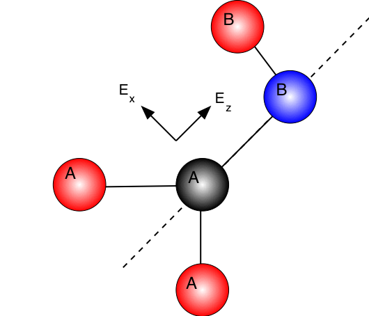
Figure 1: Schematic diagram of a molecule with internal rotation. Atoms in $A$, the top, can rotate freely with respect to atoms in $B$, the frame. The dotted line denotes the internal rotation axis,.

The study of molecules with internal rotation goes back a long way, with many theoretical developments made in the 1950’s Lin and Swalen (1959). Some recent methodology can be found in a review by Kleiner Kleiner (2010). The basic set-up is shown schematically in figure 1. The molecule consists of two sets of atoms $A$ and $B$ which are free to rotate independently about a common molecular axis, with angle $\alpha$ between $A$ and $B$. The molecule frame is centred on the centre of mass with $z$ axis aligned parallel to the internal rotation axis Lin and Swalen (1959) and the $x$ axis is fixed with respect to $B$. The molecule coordinates are the Euler angles $\theta$, $\phi$ and $\psi$ of the molecular frame and the internal rotation $\alpha$. The approach adopted here is to develop concepts which are, as far as possible, independent of the choice of coordinates.

The mass the molecule is denoted by $M$ and the mass of $A$ by $M_{A}$. A vector $\sigma$ runs from the centre of mass to a chosen point $C$ on the molecular axis so that the locations of the individual nuclei are given by ${\bf r}_{n}=R(\theta,\phi,\psi)(\mbox{\boldmath$\sigma$}+R(0,0,\alpha_{n}){\bf a}_{n})$, where rotation matrices $R$ act on the vectors ${\bf a}_{n}$ fixed to $A$ or $B$, and $\alpha_{n}=\alpha$ when $n\in A$, $\alpha_{n}=0$ otherwise. The total moment of inertia of the molecule $I_{ij}$ is computed in the molecule frame with origin at the centre of mass, whilst the moments of inertia of A and B are more conveniently centred on the rotation axis at C.

The rotational kinetic energy of the molecule is Quade and Lin (1963); Quade (1966)

$$T=\frac{1}{2}I_{ij}\omega^{i}\omega^{j}+\rho_{i}\omega^{i}\dot{\alpha}+\frac{1}{2}I^{A}\dot{\alpha}^{2},$$ (5)

where $\omega^{i}$ is the angular velocity in the body frame, and the components are given by

$$I_{ij} = I^{A}{}_{ij}+I^{B}{}_{ij}-M({\bf E}_{i}\times\mbox{\boldmath$\sigma$})\cdot({\bf E}_{j}\times\mbox{\boldmath$\sigma$})$$ (6)

$$\rho_{i} = I^{A}{}_{iz}+M_{A}({\bf E}_{i}\times\mbox{\boldmath$\sigma$})\cdot({\bf E}_{z}\times\mbox{\boldmath$\rho_{A}$})$$ (7)

$$I^{A} = I^{A}{}_{zz}-M_{A}^{2}({\bf E}_{z}\times\mbox{\boldmath$\rho_{A}$})\cdot({\bf E}_{z}\times\mbox{\boldmath$\rho_{A}$})/M.$$ (8)

The vector $\rho_{A}$ runs from the point C on the rotation axis to the centre of mass of $A$.

The kinetic energy defines an intrinsic metric $g$ on the four dimensional configuration space. It is convenient to use the same notation $\omega^{i}$ for the differentials associated with the angular velocities, and $\omega^{\alpha}=d\alpha$ for the internal rotation. The metric can be written in the form

$$g=I_{ij}(\omega^{i}+\rho^{i}\omega^{\alpha})(\omega^{j}+\rho^{j}\omega^{\alpha})+N^{2}\omega^{\alpha\,2}.$$ (9)

Comparison with the kinetic energy shows that the vector $\rho^{i}=I^{ij}\rho_{j}$ and $N^{2}=I^{A}-I^{ij}\rho_{i}\rho_{j}$, where $I^{ij}$ is the matrix inverse of $I_{ij}$. The metric (9) has a three dimensional symmetry group which can be classified under the Bianchi classification of Lie algebras as Bianchi type IX Kundt (2003). This symmetry corresponds to rotating the molecular coordinate frame and allows us to change frame to another coordinate system whenever this is convenient. (This has nothing to do with the molecular symmetry group). Bianchi IX metrics also arise in the study of cosmological models Ryan and Shepley (1975). An anisotropic inertia tensor corresponds to an anisotropic cosmological model, and the internal angle is analogous to the cosmological time parameter, though a change from space to spacetime requires replacing $N^{2}$ by $-N^{2}$.

The kinetic term in the effective Hamiltonian (1) is given by the Laplacian,

$$-\frac{\hbar^{2}}{2}\nabla^{2}=\frac{1}{2}I^{ij}p_{i}p_{j}+|I|^{-1/2}F^{1/2}\left(p_{\alpha}-\rho^{i}p_{i}\right)|I|^{1/2}F^{1/2}\left(p_{\alpha}-\rho^{j}p_{j}\right),$$ (10)

where $F=1/2N^{2}$ and $p_{i}$ are the usual angular momenta. The momenta can also be written as $p_{a}=-i\hbar D_{a}$, where $D_{i}$ are the derivatives defined by the duality relations $\omega^{i}(D_{j})=\delta^{i}{}_{j}$ and $D_{\alpha}=\partial/\partial\alpha$. The ordering of the derivatives in this way ensures that the quantum theory preserves the Bianchi IX symmetry. Note that whenever the top part part of the molecule has $C_{n>2}$ symmetry about the rotation axis, then $F$ and $|I|$ and $\rho^{i}$ are all independent of the internal angle and the factor ordering becomes unimportant. In this case it makes sense to choose a frame in which selected components of $I_{ij}$ or $\rho^{i}$ vanish Lin and Swalen (1959).

The geometrical potential terms in the effective Hamiltonian are invariant under the frame rotations up to relocation of the origin of the internal rotation angle. The curvature scalar may be calculated using general formulae for Bianchi-type metrics in Ryan and Shepley Ryan and Shepley (1975). If ${\bf I}$ denotes the inertia matrix, then

$$R = -2F^{1/2}D_{\alpha}{\rm tr}\left({\bf I}^{-1}F^{1/2}D_{\alpha}{\bf I}\right)-\frac{1}{2}F\left({\rm tr}\,{\bf I}^{-1}D_{\alpha}{\bf I}\right)^{2}-\frac{1}{2}F\,{\rm tr}\left({\bf I}^{-1}D_{\alpha}{\bf I}\right)^{2}$$ (12)

$$+2\,{\rm tr}\,{\bf I}^{-1}+\frac{1}{4}{\rm tr}\,{\bf I}\,{\rm tr}\,{\bf I}^{-2}-\frac{1}{4}{\rm tr}\,{\bf I}\,({\rm tr}\,{\bf I}^{-1})^{2}.$$

The remaining extrinsic curvature terms can be related to the tangent vectors ${\bf e}_{a}=D_{a}{\bf r}_{n}$, $a=i$ or $\alpha$. The components of the intrinsic metric (9) are

$$g_{ab}=\sum_{n}m_{n}(D_{a}{\bf r}_{n})\cdot(D_{b}{\bf r}_{n})$$

The extrinsic curvature $K_{ab}$ is the normal projection of $D_{b}{\bf e}_{a}$,

$$K_{ab}=D_{b}D_{a}{\bf r}_{n}-g^{cd}\sum_{p}m_{p}(D_{b}D_{a}{\bf r}_{p})\cdot D_{c}{\bf r}_{p}\,D_{d}{\bf r}_{n}.$$ (13)

Its square is given by

$$K^{2}=g^{ab}g^{cd}\kappa_{abcd}-g^{ab}g^{cd}g^{ef}\kappa_{abe}\kappa_{cdf}.$$ (14)

where

$$\kappa_{abcd} = \sum_{n}m_{n}(D_{a}D_{b}{\bf r}_{n})\cdot(D_{c}D_{d}{\bf r}_{n}),$$ (15)

$$\kappa_{abc} = \sum_{n}m_{n}(D_{a}D_{b}{\bf r}_{n})\cdot D_{c}{\bf r}_{n}.$$ (16)

It is possible to express both of these tensors entirely in terms of the inertia tensors $I_{ij}$, $\rho_{i}$ and $I^{A}$. If there is a $C_{n>2}$ symmetry about the rotation axis then the inertial tensors and the curvature terms are constant. The interesting cases are therefore ones in which the molecule has at most a $C_{2}$ symmetry or in which the rotation axis is displaced from the axis of symmetry.

The potential in the effective Hamiltonian has contributions from the zero-point vibrational energy and the extra vibrational term in (2), which uses the covariant derivatives of the normal modes

$$\nabla_{i}\nu_{IJ}=(\nu_{I}-\nu_{J})\sum_{n}m_{n}R(0,0,\alpha_{n})\,{\bf d}_{nI}\times{\bf d}_{nJ}.$$ (17)

${\bf d}_{nI}$ are the displacements of molecule $n$ in normal mode $I$ with frequency $\nu_{I}$. This paper focusses on the less familiar geometrical terms, and the analysis given above shows that these have no dependence on the vibrational modes.

For the most general type of asymmetric rotor, in an arbitrary molecular frame, the geometric potential has a Fourier series expansion

$$V_{R}=\sum_{n=0}^{\infty}\left(a_{n}\cos\,n\alpha+b_{n}\sin\,n\alpha\right).$$

The cofficients can be combined to form a set which is indepenent of the frame, by taking $V_{0}=a_{0}$ and $V_{n}=2(a_{n}^{2}+b_{n}^{2})^{1/2}.$ These reduce to the usual Fourrier series coefficients when $b_{n}=0$, which happens, for example, if a reflection symmetry has been used to align the origin of the molecular frame.

Table 1: Fourrier series components of the geometric potential term $V_{R}=\frac{1}{4}\hbar^{2}R-\frac{1}{8}\hbar^{2}K^{2}$ and the kinetic function $F$ for a selection of molecules with internal rotation. These use identical molecular structures for each isotopomer using data obtained from Linstrom and Mallard (2013).

	Isotopomer	$V_{1}/hc\,(cm^{-1})$	$V_{2}/hc\,(cm^{-1})$	$V_{3}/hc\,(cm^{-1})$	$F_{0}/hc\,(cm^{-1})$	$F_{1}/hc\,(cm^{-1})$	$F_{2}/hc\,(cm^{-1})$
Ethylene	${\rm CH_{2}CH_{2}}$	0.000	0.279	0.000	21.964	0.000	0.000
	${\rm CH_{2}CD_{2}}$	0.000	0.284	0.000	16.476	0.000	0.000
	CHDCHD	0.126	0.393	0.003	15.203	0.496	0.048
Methanol	${\rm CH_{3}OH}$	0.036	0.001	0.000	27.639	0.129	0.000
	${\rm CH_{2}DOH}$	0.105	0.154	0.000	26.392	0.496	0.060
	${\rm CH_{2}D{}^{18}OH}$	0.101	0.137	0.000	26.216	0.470	0.051
	${\rm CHD_{2}OH}$	0.040	0.110	0.000	25.480	0.244	0.050
	${\rm CHD_{2}OD}$	0.040	0.126	0.000	15.187	0.244	0.049
Peroxymethyl	${\rm CH_{3}O_{2}}$	0.000	0.000	0.000	6.845	0.000	0.000
	${\rm CH_{2}DO_{2}}$	0.043	0.291	0.001	5.546	0.359	0.062
	${\rm CHD_{2}O_{2}}$	0.015	0.185	0.001	4.684	0.232	0.009
Nitrosomethane	${\rm CH_{3}NO}$	0.017	0.039	0.000	7.680	0.037	0.007
	${\rm CH_{2}DNO}$	0.052	0.297	0.000	6.390	0.412	0.082
	${\rm CHD_{2}NO}$	0.037	0.238	0.001	5.562	0.302	0.047
Acetaldehyde	${\rm CH_{3}CHO}$	0.011	0.001	0.000	7.744	0.034	0.000
	${\rm CH_{2}DCHO}$	0.064	0.210	0.001	6.431	0.408	0.059
	${\rm CHD_{2}CHO}$	0.041	0.140	0.001	5.589	0.301	0.023

Results for the geometric potentials $V_{R}$ and the kinetic term $F$ (see eq. (10)) of a selection of molecules with isotoptic replacements are presented in table 1. Breaking $C_{3}$ symmetry results in geometric terms which are typically in the range 0.1-0.3 $\hbox{cm}^{-1}$. Some of the molecules have non-vanishing potentials even though they posses $C_{3}$ symmetry, due to misalignment of the rotation axis and the axis of symmetry. The components $V_{1}$ and $F_{1}$ split doublet into triplet spectral lines in the rotational spectra of molecules such as ${\rm CD_{2}HCHO}$ Kilb et al. (1957). The splitting due to the $F_{1}$ (kinetic) term is known to be insufficient to explain the data without adjusting the alignment of the rotation axis Quade and Lin (1963) or introducing empirical centrifugal distortion terms Turner and Cox (1976).

With large asymmetry, for example with the halogenated organic molecules in table 2, the geometrical potenials can be as high as 1-2 $\hbox{cm}^{-1}$.

Table 2: Fourrier series components of the geometric potential term $V_{R}=\frac{1}{4}\hbar^{2}R-\frac{1}{8}\hbar^{2}K^{2}$ and the kinetic function $F$ for a selection of halogenated organic molecules with internal rotation.

	Halogen substituent	$V_{1}/hc\,(cm^{-1})$	$V_{2}/hc\,(cm^{-1})$	$V_{3}/hc\,(cm^{-1})$	$F_{0}/hc\,(cm^{-1})$	$F_{1}/hc\,(cm^{-1})$	$F_{2}/hc\,(cm^{-1})$
Ethylene	${\rm CF_{2}CH_{2}}$	0.000	0.275	0.000	11.555	0.000	0.000
	${\rm CHFCHF}$	0.594	1.941	0.054	5.291	2.530	1.055
Methanol	${\rm CHF_{2}HO}$	0.284	0.601	0.005	22.353	0.233	0.440
	${\rm CH_{2}FHO}$	0.526	1.090	0.002	23.790	1.318	0.440
	${\rm CH_{2}FFO}$	0.330	1.573	0.059	4.106	1.155	0.746
Peroxymethyl	${\rm CH_{2}FO_{2}}$	0.178	1.378	0.057	2.776	0.899	0.587
	${\rm CHF_{2}O_{2}}$	0.145	0.472	0.022	1.665	0.034	0.181
Nitrosomethane	${\rm CH_{2}FNO}$	0.274	1.542	0.063	3.572	1.084	0.736
	${\rm CHF_{2}NO}$	0.189	0.689	0.038	2.425	0.105	0.398
	${\rm CF_{3}NO}$	0.019	0.034	0.000	2.043	0.050	0.024
Acetaldehyde	${\rm CH_{2}FCHO}$	0.266	1.128	0.032	3.637	1.120	0.559
	${\rm CHF_{2}CHO}$	0.135	0.473	0.017	2.485	0.057	0.279

The usefullness, or otherwise, of these geometrical terms is largely dependent on the accuracy of the calculations for much larger Born-Openhiemer and vibrational potential terms. The ab initio calculations for acetaldehyde in Refs. Csaszar et al. (2004); Allen et al. (2006) are said to have an accuracy of around 2 $\hbox{cm}^{-1}$ for the coefficient $V_{3}$. These calculations include the zero-point vibrational energy $\hbar{\rm tr}\,\nu/2$. Note that, in addition to the zero point energy and the geometrical potential there should also be the extra vibrational term in the effective Hamiltonian Moss and Shiiki (2000),

$$\frac{\hbar^{2}}{16}g^{ab}{\rm tr}\left(\nu^{-1}\nabla_{a}\nu\cdot\nu^{-1}\nabla_{b}\nu\right).$$ (18)

Finally, there are numerical schemes available which go beyond the Born-Openheimer approximation by quantising the nuclei as well as the electrons (e.g. Ishimoto et al. (2008)). These methods give the energy of the ground state of the molecule, and by comparing different equilibium configurations for the internal rotation they can also give an effective barrier height, but they do not so far give information about the Fourier components of the effective potential.

References

- Jensen and Koppe (1971) H. Jensen and H. Koppe, Annals Phys. 63, 586 (1971).
- Maraner (1995) P. Maraner, J.Phys. A28, 2939 (1995), arXiv:hep-th/9409080 [hep-th] .
- Moss and Shiiki (2000) I. G. Moss and N. Shiiki, Nucl.Phys. B565, 345 (2000), arXiv:hep-th/9904023 [hep-th] .
- Schuster and Jaffe (2003) P. Schuster and R. Jaffe, Annals Phys. 307, 132 (2003), arXiv:hep-th/0302216 [hep-th] .
- Watson (1967) J. K. G. Watson, The Journal of Chemical Physics 46, 1935 (1967).
- Watson (1968) J. K. Watson, Molecular Physics 15, 479 (1968), http://www.tandfonline.com/doi/pdf/10.1080/00268976800101381 .
- Kleiner (2010) I. Kleiner, Journal of Molecular Spectroscopy 260, 1 (2010).
- Duan and Takagi (1995) Y.-B. Duan and K. Takagi, Physics Letters A 207, 203 (1995).
- Duan et al. (1996) Y.-B. Duan, H.-M. Zhang, and K. Takagi, The Journal of Chemical Physics 104, 3914 (1996).
- Duan et al. (1999) Y.-B. Duan, L. Wang, X. T. Wu, I. Mukhopadhyay, and K. Takagi, The Journal of Chemical Physics 111, 2385 (1999).
- Xu et al. (1999) L.-H. Xu, R. M. Lees, and J. T. Hougen, The Journal of Chemical Physics 110, 3835 (1999).
- Wang et al. (2003) L. Wang, Y.-B. Duan, R. Wang, G. Duan, I. Mukhopadhyay, D. S. Perry, and K. Takagi, Chemical Physics 292, 23 (2003).
- Lin and Swalen (1959) C. C. Lin and J. D. Swalen, Rev. Mod. Phys. 31, 841 (1959).
- Quade and Lin (1963) C. R. Quade and C. C. Lin, The Journal of Chemical Physics 38, 540 (1963).
- Quade (1966) C. R. Quade, The Journal of Chemical Physics 44, 2512 (1966).
- Kundt (2003) W. Kundt, General Relativity and Gravitation 35, 491 (2003).
- Ryan and Shepley (1975) M. Ryan and L. Shepley, Homogeneous Relativistic Cosmologies, Princeton Series in Physics (Princeton University Press, 1975).
- Linstrom and Mallard (2013) P. J. Linstrom and W. G. Mallard, NIST Standard Reference Database Number 101, NIST Chemistry WebBook (National Institute of Standards and Technology, Gaithersburg, 2013).
- Kilb et al. (1957) R. W. Kilb, C. C. Lin, and J. E. B. Wilson, The Journal of Chemical Physics 26, 1695 (1957).
- Turner and Cox (1976) P. H. Turner and A. Cox, Chemical Physics Letters 42, 84 (1976).
- Csaszar et al. (2004) A. G. Csaszar, V. Szalay, and M. L. Senent, The Journal of Chemical Physics 120, 1203 (2004).
- Allen et al. (2006) W. D. Allen, A. Bodi, V. Szalay, and A. G. Csaszar, The Journal of Chemical Physics 124, 224310 (2006).
- Ishimoto et al. (2008) T. Ishimoto, Y. Ishihara, H. Teramae, M. Baba, and U. Nagashima, The Journal of Chemical Physics 128, 184309 (2008).