Sampling exactly from the normal distribution

Abstract

An algorithm for sampling exactly from the normal distribution is given. The algorithm reads some number of uniformly distributed random digits in a given base and generates an initial portion of the representation of a normal deviate in the same base. Thereafter, uniform random digits are copied directly into the representation of the normal deviate. Thus, in contrast to existing methods, it is possible to generate normal deviates exactly rounded to any precision with a mean cost that scales linearly in the precision. The method performs no extended precision arithmetic, calls no transcendental functions, and, indeed, uses no floating point arithmetic whatsoever; it uses only simple integer operations. It can easily be adapted to sample exactly from the discrete normal distribution whose parameters are rational numbers.

1 Introduction

Random variables with a normal density,

$$\phi(x)=\frac{\exp(-x^{2}/2)}{\sqrt{2\pi}},$$

are widely used in Monte Carlo simulations. Over the past sixty years, scores of algorithms for generating such normal deviates have been published (Thomas et al., 2007). In this paper, I give another algorithm, Algorithm N, with the distinguishing feature that, given a source of uniformly distributed random digits in some base $b$, it generates exact normal deviates. In order to make the meaning of “exact” precise, consider Table 1 which shows the operation of the algorithm using $b=10$.

The first column shows the random digits used by the algorithm, which, in this example, are taken from successive lines of the table of random digits produced by the RAND Corporation (1955), beginning at line 9077. Referring to the first line of this table, the algorithm completes after reading the 7 random decimal digits, $9148686$, from the source and produces $+1.6$ as the initial portion of the decimal representation of a normal deviate. At this point, random digits can be copied directly from the input to the output, indicated by the ellipses ($\ldots$) in the table; thus $+1.6\ldots$ represents a uniform random sample in the range $(1.6,1.7)$. The next digits of the random sequence are $685171\ldots$, allowing the normal deviate to be exactly rounded to 6 decimal digits as $1.668517$. I call the intermediate result, e.g., $+1.6\ldots$, a “u-rand”. This can be thought of as a partially sampled uniform deviate. However, in conjunction which a source of random digits it is better to think of it as a compact representation of an arbitrary precision random deviate. (The results in Table 1 are not “typical,” because the starting line in the table of random digits was specifically chosen to limit the number of random digits used.)

Table 1: Sample input and output for Algorithm N with $b=10$. The input consists of uniformly distributed random decimal digits. The algorithm reads the random digits before the vertical bar and produces a normal deviate as a u-rand (given in the second column), which is an initial portion of the decimal representation of the normal deviate. Thereafter random digits are copied directly from the input (the digits after the vertical bar) into the decimal fraction of the u-rand. The third column shows the result of adding enough digits to allow the deviate to be rounded to 6 decimal digits; the parenthetical sign indicates whether the magnitude of true deviate is greater $(+)$ or smaller $(-)$ than the rounded result.

input	u-rand	rounded
$9148686\mid 685171\ldots$	$+1.6\ldots$	$+1.668517(+)$
$2708\mid 5545979\ldots$	$+0\ldots$	$+0.554598(-)$
$501446297\mid 43871\ldots$	$+1.42\ldots$	$+1.424387(+)$
$065130319777860\mid 96289\ldots$	$-0.76\ldots$	$-0.769629(-)$
$2736\mid 0659086\ldots$	$+0\ldots$	$+0.065909(-)$

It’s clear from this example that the method can be used to generate deviates that satisfy the conditions of “ideal approximation” (Monahan, 1985), namely that the algorithm is equivalent to sampling a real number from the normal distribution and rounding it to the nearest representable floating point number. Furthermore, for applications requiring high precision normal deviates, the new algorithm offers perfect scaling: there’s an amortized constant cost to producing the initial portion of the normal deviate; but, thereafter, the digits can be added to the result at a rate limited only by the cost of producing and copying the random digits. Other sampling methods are frequently referred to as “exact,” for example the polar method (Box and Muller, 1958) and the ratio method (Kinderman and Monahan, 1977); but these are merely “accurate to round off” which, in practice, means only that the accuracy is commensurate with the precision of the floating point number system. It’s possible to convert such algorithms to obtain correctly rounded deviates; but this inevitably involves the use of extended precision arithmetic. I will show, in Sec. 5, that Algorithm N performs substantially better.

It’s not immediately obvious that such an algorithm for exact sampling is possible. However, in the early years of the era of modern computing, von Neumann (1951) presented a remarkably simple algorithm for sampling from the exponential density, in which “the machine has in effect computed a logarithm by performing only discriminations on the relative magnitude of numbers in $(0,1)$.” Knuth and Yao (1976) showed that the algorithm can easily be adapted to generate exponential deviates which are exact; and the resulting method was extensively analyzed by Flajolet and Saheb (1986). Several authors have generalized von Neumann’s algorithm (Forsythe, 1972; Ahrens and Dieter, 1973; Brent, 1974; Monahan, 1979). However, these efforts entail using ordinary floating point arithmetic and thus the methods do not generate exact deviates.

In this paper, I show that von Neumann’s algorithm can be extended to sample exactly from the unit normal and discrete normal distributions. Although the resulting algorithms are unlikely to displace existing methods for most applications, it provides a nearly optimal method for generating normal deviates at arbitrary precision. In addition, the ability to sample exactly from the discrete normal has applications to cryptography because the security of cryptographic systems requires that any random sampling be very accurate. Finally, the method is of theoretical interest as an example of an algorithm where exact transcendental results can be achieved with simple integer arithmetic.

Implementations of the algorithms given in this paper are available in ExRandom, a small “header only” library for C++11, available at http://exrandom.sf.net/, and in version 3.2.0 of MPFR (2014).

2 von Neumann’s algorithm

I begin by reviewing von Neummann’s algorithm, because this is the basis of the method for sampling from the normal distribution.

Algorithm V (von Neumann).   Samples $E$ from the exponential distribution $e^{-x}$ for $x>0$.

V1.[Initialize rejection count.] Set $l\leftarrow 0$.

V2.[Sample fraction.] Set $x\leftarrow U$, where $U$ is a uniform deviate $U\in(0,1)$.

V3.[Generate a run.] Sample uniform deviates $U_{1},U_{2},\ldots$ and determine the maximum value $n\geq 0$ such that $x>U_{1}>U_{2}>\ldots>U_{n}$.

V4.[Test length of run.] If $n$ is odd set, $l\leftarrow l+1$ and go to step V2.

V5.[Combine integer and fraction.] Otherwise ($n$ is even), set $y\leftarrow l+x$.

V6.[Return result.] Set $E\leftarrow y$.  

(Because the algorithm generates continuous random deviates, there’s no distinction between the inequalities $x\geq 0$ and $x>0$ or the intervals $(0,1)$ and $[0,1]$.) According to von Neumann, this algorithm was suggested by the game of Black Jack and this connection is made plain in the slightly different formulation given in Abramowitz and Stegun (1964, §26.8.6.c(2)).

The crucial step of the algorithm is V3, which is discussed in some detail by Knuth (1998, §3.4.1.C(3)). The probability that $U_{1},\ldots,U_{n}$ are all less than $x$ is $x^{n}$ (provided that $x\in[0,1]$). The probability that, in addition, they are in descending order (one of the possible $n!$ permutations) is $x^{n}/n!$. For the condition to hold for a sequence of $n+1$ numbers, it must hold for the first $n$ of them; therefore the probability that the length of the longest decreasing sequence is $n$ is $x^{n}/n!-x^{n+1}/(n+1)!$. For a given $x$, the probability that $n$ is even is

$$1-x+\frac{x^{2}}{2!}-\frac{x^{3}}{3!}+\ldots=e^{-x},$$

while the probability that $n$ is odd (averaged over $x$) is $1-\int_{0}^{1}e^{-x}\,\mathrm{d}x=e^{-1}$. Thus the probability that the algorithm terminates with a particular value of $l$ and $x$ is $\exp\bigl{(}-(l+x)\bigr{)}$ as required.

On average, this algorithm requires $e^{2}/(e-1)\approx 4.30$ uniform deviates; in effect, the algorithm sums all the terms in the Taylor series for $e^{-x}$ in a finite mean time. Conventionally, $U$ would be sampled from the subset of reals which are representable as double precision numbers; in this case, the results would be only approximately equivalent to sampling exactly from the exponential distribution and rounding the results to the closest floating point number.

However, if we represent the uniform deviates by u-rands, it is quite easy to make the algorithm exact in the sense discussed in connection with Table 1 in Sec. 1. A u-rand can be represented in base $b$ as

$$s(n+0.d_{0}d_{1}\ldots d_{L-1}+\ldots),$$

where $s=\pm 1$, $n$ and $L$ are non-negative integers, $d_{l}$ are digits in $[0,b)$, and the fraction is written in ordinary positional notation. Only the first $L$ digits of the fraction have been sampled and the final ellipsis represents the digits which are not yet known, i.e., it represents a sample from $b^{-L}U$. Only a small number of operations need to be implemented on u-rands to realize Algorithm V. The assignment $x\leftarrow U$ in step V2 corresponds to $s\leftarrow 1$, $n\leftarrow 0$, $L\leftarrow 0$. The operation $l+x$ in step V5 is just $n\leftarrow l$. This just leaves the comparisons between u-rands in step V3. In this case, we have $s=1$ and $n=0$ for both u-rands, so only the fractions need to be compared. The digits are compared starting at position $0$ and if they are different, the comparison can be made; if not, the next digits are compared. During this process, digits sampled uniformly from $[0,b)$ are added to the fractions and $L$ is incremented as necessary; typically, the comparisons can be made examining only a few digits of each operand.

We shall need to add a few additional operations on u-rands to implement the additional algorithms presented in this paper: negation ($x\leftarrow-x$), comparisons with a rational ($x<u/v$), incrementing by one half ($x\leftarrow x+\frac{1}{2}$); these are easily accomplished (with the proviso that $b$ be even for the last operation). We also need to be able to extract from a u-rand the value rounded to the closest floating point number at some precision, sampling, if necessary, additional digits. This is straightforward if $b$ is a power of two; all rounding modes can be supported (and the process provides a flag indicating the direction of the rounding). Finally, it is easy to produce printed representations of the u-rand itself (e.g., ‘‘$+1.6\ldots$’’) and of a correctly rounded fixed point representation in base $b$ (for examples, see Table 1). In this connection, note that by using $b=10$ we are able to produce exactly rounding decimal representations of normal deviates without any radix conversions.

It’s possible to make von Neumann’s algorithm slightly more efficient by using early rejection.

Algorithm E (improved von Neumann).   Improved algorithm for sampling $E$ from a distribution with density $e^{-x}$ for $x>0$.

E1.[Initialize rejection count.] Set $l\leftarrow 0$.

E2.[Sample fraction.] Set $x\leftarrow U$, where $U$ is a uniform deviate $U\in(0,1)$.

E3.[Early rejection.] If $x>\frac{1}{2}$, set $l\leftarrow l+1$ and go to step E2.

E4.[von Neumann’s step V3.] Sample uniform deviates $U_{1},U_{2},\ldots$ and determine the maximum value $n\geq 0$ such that $x>U_{1}>U_{2}>\ldots>U_{n}$.

E5.[Test length of run.] If $n$ is odd, set $l\leftarrow l+1$ and go to step E2.

E6.[Combine integer and fraction.] Otherwise ($n$ is even), set $y\leftarrow\frac{1}{2}l+x$.

E7.[Return result.] Set $E\leftarrow y$.  

The early rejection step results in lowering the mean number of uniform deviates required to $e/(\sqrt{e}-1)\approx 4.19$.

Von Neumann’s algorithm can be adapted to generate a Bernoulli random variable with probability $1/\sqrt{e}$, as follows.

Algorithm H (a half exponential Bernoulli trial).   Generates a Bernoulli random value $H$ which is true with probability $1/\sqrt{e}$.

H1.[Generate a run.] Sample uniform deviates $U_{1},U_{2},\ldots$ and determine the maximum value $n\geq 0$ such that $\frac{1}{2}>U_{1}>U_{2}>\ldots>U_{n}$.

H2.[Test length of run.] Set $H\leftarrow(\text{$n$ is even}).$  

On average, the algorithm uses $\frac{1}{2}e/(\sqrt{e}-1)$ (resp. $\frac{1}{2}e$) uniform deviates if the result is false (resp. true); the overall weighted average is $\sqrt{e}$. Both Algorithms E and H can be implemented using u-rands and so can deliver exact results. Algorithm H will be used for sampling from the normal distribution.

3 Sampling from the normal distribution

Here I tackle the problem of sampling normal deviates using u-rands. Although, I didn’t realize it at the time, the method I developed is closely related to the algorithm given by Kahn (1956, p. 41); see also Abramowitz and Stegun (1964, §26.8.6.a(4)). This is

Algorithm K (Kahn).   Sample $N$ from a unit normal distribution $\phi(x)$ using Kahn’s method.

K1.[Sample absolute value of deviate $y$.] Set $y\leftarrow E$ where $E$ is an exponential deviate.

K2.[Adjust relative probability of $y$ by rejection.] Sample $z\leftarrow E$ and accept $y$ if $z>{\frac{1}{2}(y-1)^{2}}$; otherwise go to step K1. (For a given $y$, the probability of acceptance $\exp\bigl{(}-\frac{1}{2}(y-1)^{2}\bigr{)}$. Averaging over $y$, the probability of acceptance is $\sqrt{\pi/(2e)}\approx 0.76$.)

K3.[Assign a sign.] With equal probabilities, set $x\leftarrow\pm y$.

K4.[Return result.] Set $N\leftarrow x$.  

A problematic step here is K2, which requires performing arithmetic on $y$. In order to avoid this, I found it necessary to sample separately the integer and factional parts of $y$, leading to the following skeleton of an algorithm.

Algorithm N (normal sampling).   Sample $N$ from a unit normal distribution $\phi(x)$ using a rejection method.

N1.[Sample integer part of deviate $k$.] Select integer $k\geq 0$ with probability $\exp(-\frac{1}{2}k)(1-1/\sqrt{e})$.

N2.[Adjust relative probability of $k$ by rejection.] Accept $k$ with probability $\exp\bigl{(}-\frac{1}{2}k(k-1)\bigr{)}$; otherwise go to step N1.

N3.[Sample fractional part of deviate $x$.] Set $x\leftarrow U$, where $U$ is a uniform deviate $U\in(0,1)$.

N4.[Adjust relative probability of $x$ by rejection.] Accept $x$ with probability $\exp\bigl{(}-\frac{1}{2}x(2k+x)\bigr{)}$; otherwise go to step N1.

N5.[Combine integer and fraction.] Set $y\leftarrow k+x$.

N6.[Assign a sign.] With probability $\frac{1}{2}$, set $y\leftarrow-y$.

N7.[Return result.] Set $N\leftarrow y$.  

The analysis of this algorithm is similar to that for Kahn’s method. After step N2, the relative probability density of $k$ is $\exp(-\frac{1}{2}k)\times{\exp\bigl{(}-\frac{1}{2}k(k-1)\bigr{)}}=\exp(-\frac{1}{2}k^{2})$ for $k\geq 0$; after step N4, the relative probability of $[k,x]$ is $\exp(-\frac{1}{2}k^{2})\times\exp\bigl{(}-\frac{1}{2}x(2k+x)\bigr{)}={\exp\bigl{(}-\frac{1}{2}(k+x)^{2}\bigr{)}}$ for $k\geq 0$ and $x\in(0,1)$. From this, it follows that the returned value of $x$ has a Gaussian distribution, $\phi(x)$. Step N2 always succeeds for $k=0$ and $1$, the two most common cases. Overall, the probability that step N2 succeeds is $(1-1/\sqrt{e})G\approx 0.690$ where $G=\sum_{k=0}^{\infty}\exp(-\frac{1}{2}k^{2})\approx 1.753$. Similarly, step N4 succeeds with probability $\sqrt{\pi/2}/G\approx 0.715$. Thus, step N1 is executed $\sqrt{2/\pi}/(1-1/\sqrt{e})\approx 2.03$ times on average.

Steps N1 and N2 can be expressed in terms of half exponential Bernoulli trials $H$ with

Steps N1 and N2 in terms of $H$.

N1.[Test $H$ until failure.] Generate a sequence of Bernoulli deviates $H_{1},H_{2},\ldots$ and determine the largest $k\geq 0$ such that $H_{1},H_{2},\ldots,H_{k}$ are all $\mathrm{true}$.

N2.[Make $k(k-1)$ tests of $H$.] Set $k^{\prime}\leftarrow k(k-1)$ and generate up to $k^{\prime}$ Bernoulli deviates $H_{1},H_{2},\ldots,H_{k^{\prime}}$. Accept $k$ if $H_{i}$ is $\mathrm{true}$ for all $i\in[1,k^{\prime}]$; otherwise go to step N1.

Of the remaining steps only step N4 presents a challenge. This is changed to

Rewriting step N4.

N4.[Break N4 into $k+1$ steps.] Perform up to $k+1$ Bernoulli trials, $B_{1},B_{2},\ldots,B_{k+1}$, each with probability ${\exp\bigl{(}-x(2k+x)/(2k+2)\bigr{)}}$. Accept $x$ if $B_{i}$ is $\mathrm{true}$ for all $i\in[1,k+1]$; otherwise go to step N1.

This transformation of N4 is motivated by the requirement in the proof of von Neumann’s method that $x\in[0,1]$. Repeating the trial $k+1$ times means that the argument to the exponential in the original step N4 is divided by $k+1$; the maximum value of $x(2k+x)/(2k+2)$ (as $x$ is varied) is $(2k+1)/(2k+2)<1$.

In order to carry out a Bernoulli trial $B$, I generalize von Neumann’s procedure.

Algorithm B (generalizing von Neumann’s step V3).   A Bernoulli trial with probability $\exp\bigl{(}-x(2k+x)/{(2k+2)}\bigr{)}$. Sample two sets of uniform deviates $U_{1},U_{2},\ldots$ and $V_{1},\allowbreak V_{2},\ldots$ and determine the maximum value $n\geq 0$ such that $x>U_{1}>U_{2}>\ldots>U_{n}$ and $V_{i}<(2k+x)/(2k+2)$ for all $i\in[1,n]$.

B1.[Initialize loop.] Set $y\leftarrow x$, $n\leftarrow 0$.

B2.[Generate and test next samples.]
(i) Sample $z\leftarrow U$; go to step B4, unless $z<y$.
(ii) Sample $r\leftarrow U$; go to step B4, unless $r<{(2k+x)}/(2k+2)$.

B3.[Increment loop counter and repeat.] Set $y\leftarrow z$, $n\leftarrow n+1$; go to step B2.

B4.[Test length of runs.] Set $B\leftarrow(\text{$n$ is even})$.  

Without step B2(ii), steps B1 to B3 are just step V3 of von Neumann’s algorithm. Because of the additional test B2(ii), the probability that the $n$th trip through the loop succeeds is $x^{n}/n!\times{\bigl{(}(2k+x)/(2k+2)\bigr{)}^{n}}$. The requirement that $n$ be even means that $B$ succeeds with probability

$$1-x\frac{2k+x}{2k+2}+\frac{x^{2}}{2!}\biggl{(}\frac{2k+x}{2k+2}\biggr{)}^{2}-\frac{x^{3}}{3!}\biggl{(}\frac{2k+x}{2k+2}\biggr{)}^{3}+\ldots\\ =\exp\biggl{(}-x\frac{2k+x}{2k+2}\biggr{)}.$$

In order to avoid performing arithmetic on uniform deviates in step B2(ii), we remark that as $x$ varies in $(0,1)$ the right side of the inequality varies from $2k/(2k+2)$ to $(2k+1)/(2k+2)$. Thus, regardless of the values of $x$ and $r$, the test will succeed with probability $2k/(2k+2)$ and fail with probability $1/(2k+2)$. The remaining probability, $1/(2k+2)$, is divided between success and failure according to $r<x$. Thus the test $r<(2k+x)/(2k+2)$ can be replaced with

Algorithm T (the test in B2(ii)).   Perform test $T=\bigl{(}r<(2k+x)/(2k+2)\bigr{)}$ without doing arithmetic on real numbers.

T1.[Sample a selector $f$.] Set $f\leftarrow C(2k+2)$ where $C(m)$ is $-1$ with probability $1/m$, $0$ with probability $1/m$, and $1$ with probability $1-2/m$.

T2.[Act on the value of $f$.] If $f<0$, set $T\leftarrow\mathrm{false}$; else if $f>0$, set $T\leftarrow\mathrm{true}$; otherwise ($f=0$), set $T\leftarrow{(r<x)}$.  

Finally, $C(m)$ can be computed with

Algorithm C (the 3-way selector).   The choice $C(m)$, $(-1,0,1)$ with probabilities $(1/m,1/m,\allowbreak{1-2/m})$, implemented as the test $w<n/m$ where $w$ is a uniform deviate in $(0,1)$ and $n=1$ or $n=2$. For each successive digit $d$ of $w$, substitute $w=(d+w^{\prime})/b$ so that the test becomes $w^{\prime}<n^{\prime}/m$, where $n^{\prime}=bn-dm$, and exit as soon as the $n^{\prime}$ is outside the range $(0,m)$.

C1.[Set the numerators of the fractions.] Set $n_{1}\leftarrow 1$ and $n_{2}\leftarrow 2$.

C2.[Sample the next digit of $w$, $d$.] Sample $d\leftarrow D$ where $D$ is a uniformly distributed integer in $[0,b)$.

C3.[Multiply inequalities by $bm$.] Set $n_{1}\leftarrow bn_{1}-dm$ and $n_{2}\leftarrow bn_{2}-dm$.

C4.[Test the new numerators.] If $n_{1}\geq m$, set $C(m)\leftarrow-1$ and return; else if $n_{2}\leq 0$, set $C(m)\leftarrow 1$ and return; else if $n_{1}\leq 0$ and $n_{2}\geq m$, set $C(m)\leftarrow 0$ and return; otherwise, go to step C2.  

Algorithm C shows how the comparison of a u-rand with a rational $x<u/v$ can be implemented. Step B2 can now be written as

Step B2 incorporating Algorithm T.

B2.[Generate and test next samples.]
(a) Sample $z\leftarrow U$; go to step B4, unless $z<y$.
(b) Set $f\leftarrow C(2k+2)$; if $f<0$, go to step B4.
(c) If $f=0$, sample $r\leftarrow U$ and go to step B4, unless $r<x$.

The three steps here can be carried out in any order and I find that the number of random digits needed can be reduced by reversing the order of B2(a) and B2(b) whenever $k=0$.

Now step N4 has been broken down into steps that can all be carried out in terms of u-rands. In the final step, N7, the normal deviate can be returned either as a u-rand or an exactly rounded floating point number.

4 Sampling from the discrete normal distribution

In some applications, we wish to sample integers, $i$, from the discrete normal distribution,

$$\phi(i\mid\mu,\sigma)\propto\exp\biggl{[}-\frac{1}{2}\biggl{(}\frac{i-\mu}{\sigma}\biggr{)}^{2}\biggr{]},$$

which is characterized by parameters $\mu$ and $\sigma$. In the limit $\sigma\gg 1$, the mean and variance of this distribution is well approximated by $\mu$ and $\sigma^{2}$. Considering the class of integer distributions, this distribution maximizes the entropy for a given mean and variance (Kemp, 1997). Because Algorithm N is a simple rejection scheme, it is rather easy to adapt it to sample from the discrete distribution as follows:

Algorithm D (discrete normal sampling).   Sample $D$ from a discrete normal distribution $\phi(i\mid\mu,\sigma)$ using a rejection method.

D1.[Same as step N1.] Select integer $k\geq 0$ with probability $\exp(-\frac{1}{2}k)(1-1/\sqrt{e})$.

D2.[Same as step N2.] Accept $k$ with probability $\exp\bigl{(}-\frac{1}{2}k(k-1)\bigr{)}$; otherwise go to step D1.

D3.[Assign a sign.] With equal probabilities, set $s\leftarrow\pm 1$.

D4.[Sample fractional part of deviate $x$.] Set $x\leftarrow x_{0}+j/\sigma$, where $x_{0}=\bigl{(}i_{0}-(\sigma k+s\mu)\bigr{)}/\sigma$, $i_{0}=\lceil\sigma k+s\mu\rceil$, and $j$ is a random integer uniformly sampled from $\bigl{[}0,\lceil\sigma\rceil\bigr{)}$.

D5.[Ensure that $x$ is in the allowed range.] If $x\geq 1$, go to step D1. (This cannot happen if $\sigma$ is an integer.)

D6.[Avoid double counting 0.] If $k=0$, $x=0$, and $s<0$, go to step D1. (This cannot happen unless $\mu$ is an integer.)

D7.[Same as step N4.] Accept $x$ with probability $\exp\bigl{(}-\frac{1}{2}x(2k+x)\bigr{)}$; otherwise go to step D1.

D8.[Combine parts of the integer deviate.] Set $i\leftarrow s(i_{0}+j)$.

D9.[Return result.] Set $D\leftarrow i$.  

This is nearly the same as Algorithm N, except that step N3 has been replaced by steps D4--D6. These steps can be understood by matching $\phi(x)$ and $\phi(i\mid\mu,\sigma)$, identifying $s(k+x)=\bigl{(}{s(i_{0}+j)}-\mu\bigr{)}/\sigma$, and determining $i_{0}$ and $j$ such that $x\in[0,1)$. When $j=0$, $x$ takes on the value $x_{0}$ and $i_{0}$ is that integer which minimizes $x_{0}$ while maintaining the condition $x_{0}\geq 0$. Similarly the requirement that $x<1$, imposes the condition $j<\lceil\sigma\rceil$. If $\sigma$ is not an integer, then for some values of $k$ and $s$, there are only $\lfloor\sigma\rfloor$ allowed values of $j$, so, in step D5, we enforce the condition $x\in[0,1)$. Finally, in step D6, we avoid double counting the origin of the normal distribution by additionally requiring that $x\in(0,1)$ if $k=0$ and $s<0$.

Algorithm D is a straightforward modification of Algorithm N and all the steps can be carried out exactly if the parameters $\mu$ and $\sigma$ are rational. One additional function needs to be added to the machinery to handle u-rands, namely a comparison with a rational (this is needed in implementing Algorithm B because now $x$ is a rational number). See Algorithm C for how this can be implemented.

Because the probability that step D7 (i.e., step N4) succeeds is $0.715$, then for $\sigma$ large (and $b=2$), this method requires at least $(1/0.715)\log_{2}\sigma$ bits of randomness on average. We would like to reduce the multiplier of $\log_{2}\sigma$ from $1/0.715$ to $1$ to match the perfect scaling of Algorithm N. We can achieve this goal by adapting the algorithm given by Lumbroso (2013) for sampling an integer in $[0,m)$. Sufficient of his algorithm is carried out to allow the result to be returned as range of size $b^{l}$. For example, if $b=2$, sampling from $[0,9)$ returns the ranges $\{[0,8),\allowbreak[0,2),\allowbreak[2,6),\allowbreak[6,8),\allowbreak[8,9)\}$ with probabilities $\{\frac{32}{63},\allowbreak\frac{2}{21},\allowbreak\frac{4}{21},\allowbreak\frac{2}{21},\allowbreak\frac{1}{9}\}$. Thereafter the range can be narrowed, if necessary, by factors of $b$ to allow the inequality in step D7 to be evaluated. This method of sampling integers generalizes the concepts of a u-rand to apply to discrete sampling and, if Algorithm D is implemented using this technique, it exhibits perfect scaling in the limit of large $\sigma$.

As an aside, this technique of partially sampling a discrete uniform distribution allows optimization of sampling from the Bernoulli distribution with rational probability $p=u/v$. Conventionally, this is implemented by testing $u<j$ with $j$ sampled uniformly in $[0,v)$ which for $v$ large requires at least $\log_{2}v$ random bits. However if $j$ is partially sampled, the mean cost is a constant in the limit of large $v$. Similar performance is obtained with u-rands, sampling $x\leftarrow U$ and testing $x<u/v$ (and, with u-rands, this test is exact).

5 Implementation

An implementation of Algorithm N in C++11 is available in the library ExRandom. This allows the user to select the base $b$ and to access the random deviate as a u-rand or as a floating point number. The algorithm has also been wrapped into a C++11 ‘‘random number distribution’’ (Stroustrup, 2013, §40.7.3), unit_normal_distribution, which can be used as a replacement for the standard normal_distribution (with zero mean and unit variance). Several test programs are also provided, one of which performs the $\chi^{2}$ test on the output of Algorithm N, which is an essential step in validating its correctness. This test passes with $10^{10}$ samples and 50 bins of equal width in the interval $[-4,4]$ when the Mersenne Twister random number generator (Matsumoto and Nishimura, 1998), mt19937, is used as the source of random digits. (On the other hand, the test fails badly with $10^{9}$ samples using the linear congruential generator, minstd_rand0.) Algorithm N retains no state from one invocation to the next. So it is not necessary to verify the independence of the normal deviates (any lack of independence would be due to defects in the underlying random generator).

In addition, Algorithm N has also been incorporated in MPFR (2014), version 3.2.0, a library for arbitrary precision arithmetic (Fousse et al., 2007) as the function mpfr_nrandom. MPFR, version 3.1.0, already provided a function mpfr_grandom for sampling normal deviates based on the polar method (Box and Muller, 1958).

Table 2: Times (in $\mathrm{\mu s}$) for sampling from the normal distribution. The quantity $p$ is the number of bits in the fraction of the rounded floating point samples. Columns A and D use the polar method, while columns B and C use Algorithm N. Columns A and B time the C++11 random number distributions normal_distribution and unit_normal_distribution delivering results in the form of IEEE floating point numbers. Columns C and D time the routines mpfr_nrandom and mpfr_grandom which produce MPFR floating point numbers. Columns A and B are the results of averaging over $50$ million samples; the entries in Columns C and D are each the result of averaging over about $10$ seconds.

type	IEEE		MPFR
method	polar	Algorithm N		polar
$p$	A	B	C	D
$24$	$0.034$	$0.30$	$0.59$	$2.3$
$32$			$0.64$	$2.4$
$53$	$0.054$	$0.31$	$0.64$	$2.6$
$64$	$0.057$	$0.37$	$0.64$	$2.8$
$128$			$0.65$	$3.8$
$256$			$0.68$	$6.2$
$2^{10}$			$0.86$	$20$
$2^{12}$			$1.6$	$130$
$2^{14}$			$4.3$	$1300$
$2^{16}$			$15$	$13000$
$2^{18}$			$59$	$120000$
$2^{20}$			$240$	$910000$

Table 2 shows some comparative timings for producing normal deviates with a precision of $p$ bits. The tests were run on a Fedora Linux system with a $3.2\,\mathrm{GHz}$ Intel processor using the g++ compiler version 4.8.2. In all cases, the Mersenne Twister algorithm was used to generate the random digits and the implementations of Algorithm N timed here use $b=2^{32}$ to match the output of this generator. Comparing columns A and B, we see that Algorithm N is an order of magnitude slower than the polar method at producing double precision results. On the other hand (comparing columns C and D), Algorithm N is dramatically faster than mpfr_grandom at producing arbitrary precision results in the MPFR format. As expected, the scaling of the time for Algorithm N in column C is offset linear, approximately $(1+240\,p/2^{20})\,\mathrm{\mu s}$.

It is instructive to compare the two MFPR routines mpfr_grandom and mpfr_nrandom. The former provides a good illustration of how a conventional method for sampling random deviates can be implemented with guarantees on the accuracy; the working precision needs to be progressively increased; and, of course, heavy use is made of the formidable infrastructure provided by MPFR for carrying out arbitrary precision arithmetic. The final result entails computing a logarithm and extracting a square root which incur a reasonably heavy penalty as the precision is increased (the time increases roughly as $p^{1.6}$). On the other hand, mpfr_nrandom relies on MPFR only to provide the data type to hold the result and the penalty for high precision is minimal.

Table 2 times the production of normal deviates in a standard computational environment in which uniform pseudo random numbers can be produced rather rapidly. In some security applications, it may be necessary to use a slow hardware random number generator. In this case, Algorithm N can be used with $b=2$ to conserve random bits. Let $B$ be the number of bits consumed by Algorithm N and $L$ be the number of bits in the fraction of resulting u-rand. Empirically, I find that $\left<B\right>\approx 30.000$ and $\left<L\right>\approx 1.556$. The distribution of $L$ decays with an $e$-folding constant of $1/\log 2$, while that of $B$ decays more slowly with a $e$-folding constant of about $29.9$ bits. To put these results in perspective, if $10^{30}$ normal deviates were generated, then the largest result would be $\left|x\right|\sim 12$, the longest fraction would have $L\sim 100$ and at most $B\sim 2000$ bits would be needed to generate a single normal deviate.

The quantity $C=\left<B\right>-\left<L\right>\approx 28.444$ represents the ‘‘cost’’ of producing random deviates. Producing rounded fixed point normal deviates with $p$ bits in the fraction requires $C+p+1$ random bits on average; this formula applies for large $p$ (but $p\geq 10$ suffices in practice). The $1$ here accounts for the additional bit needed for rounding the result (and the rounding operation, in turn, provides an extra bit of information, namely whether the true deviate is larger or smaller than the rounded result). Producing rounded floating point normal deviates with precision $p$ requires $C-Q+p+1$ bits on average (the $1$ again accounts for the need for a rounding bit); here $Q=\left<\lfloor\log_{2}\left|x\right|\rfloor\right>+1\approx-0.417$ is the mean floating point exponent for normal deviates. Thus producing IEEE double precision floating point numbers ($p=53$) requires about $82.861$ bits per rounded deviate, on average.

When comparing Algorithm N with algorithms for other distributions, we use the toll of the algorithm defined as $T=C-H\approx 26.397$ where $H=\log_{2}\sqrt{2\pi e}\approx 2.047$ is the entropy of the normal distribution and the base-$2$ logarithm is used so that $H$ is measured in bits. A perfect sampling algorithm would have $T=0$; so the toll is a measure of how many random bits are potentially ‘‘wasted’’ by the algorithm. (Note that the entropy of the discrete distribution obtained by rounding normal deviates to the closest multiple of $2^{-p}$ is $H+p$, for $p$ large.)

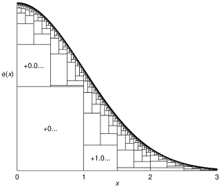
Figure 1: Algorithm N’s decomposition of the normal distribution into a set of uniform distributions with $b=2$ (shown for $x>0$). For example, the frequency with which $+0.0\ldots$ is returned is equal to the relative area of the rectangle spanning $x\in(0,\frac{1}{2})$ which is $\frac{1}{8}\sqrt{2/\pi}\approx 10\%$. This frequencies used in this figure are averaged over $10^{10}$ samples; the minimum range of the uniform distributions shown is $2^{-8}$.

A histogram of the u-rands that Algorithm N produces can be displayed in a way that illustrates how they add up to the normal distribution as shown in Fig. 1. The area assigned to each u-rand is proportional to its frequency while its base covers its range (here $b=2$). This figure is reminiscent of illustrations of the ziggurat method (Marsaglia and Tsang, 2000), which provides a fast way of sampling normal deviates by approximating the normal distribution by a static set of rectangles enabling it to return a uniform deviate in most cases. In contrast, Algorithm N dynamically generates a set rectangles which cover the normal distribution exactly, allowing it to return a uniform deviate in all cases.

The ExRandom library includes implementations of Algorithms V and E for sampling from the unit exponential distribution with interfaces that parallel those for the unit normal distribution. The C++ random number distribution unit_exponential_distribution uses Algorithm V because it is slightly faster than Algorithm E with $b=2^{32}$. This produces double precision deviates in $0.09\,\mathrm{\mu s}$ under the same conditions as in Table 2. (Algorithm V has also been added to MPFR, version 3.2.0, as mpfr_erandom.) With $b=2$, Algorithm E results in $\left<B\right>\approx 7.232$ and $\left<L\right>\approx 1.743$, so the cost is $C\approx 5.489$. For the exponential distribution, we have $H=\log_{2}e\approx 1.443$ and $Q\approx-0.333$. Thus the toll is $T=C-H\approx 4.047$ (considerably better than Algorithm N) and producing IEEE double precision numbers requires $C-Q+54\approx 59.822$ bits on average. In contrast, von Neumann’s original method, Algorithm V, has a cost $C\approx 7.262$ and a toll $T\approx 5.819$; i.e., it is less efficient than Algorithm E by about $1.772$ bits.

Finally, the ExRandom includes implementations of Algorithm D for sampling from the discrete normal distribution. The parameters $\mu$ and $\sigma$ are given as the ratio of two 32-bit integers. However some internal calculations use 64-bit integers in an effort to avoid overflow. The constructors for the class implementing this algorithm throw an exception if the parameters are such that overflow is possible. The most stringent of the checks is that $bk_{\mathrm{max}}\sigma_{\mathrm{num}}$ fits in a 64-bit word where $b$ is the base, $k_{\mathrm{max}}=50$ is how many standard deviations onto the tail of the normal distribution we want to be able to sample, and $\sigma_{\mathrm{num}}$ is the numerator of $\sigma$ when it and $\mu$ are expressed with a common denominator.

The C++11 random number distribution implementing Algorithm D uses $b=2^{16}$. The time to generate discrete normal deviates depends weakly on $\sigma$ over the range $[1.6,1.6\times 10^{6}]$ varying between $0.4\,\mathrm{\mu s}$ and $0.5\,\mathrm{\mu s}$ under the same conditions as in Table 2. With $b=2$, the toll, defined now merely as the difference between the mean number of bits to obtain a discrete normal deviate and the entropy of the distribution (in bits), is, in the limit of large $\sigma$, approximately a periodic function of $\log_{2}\sigma$ with period $1$, attaining its minimum value of about $27.9$ when $\sigma$ is a power of two and its maximum value of $31.9$ when $\sigma$ slightly exceeds a power of two.

An important potential use for Algorithm D is in cryptography, where exact sampling is often required. One such application is the ‘‘learning with errors’’ (LWE) problem (Regev, 2009), which depends on the difficulty of solving a system of over-determined linear equations over the field of integers when the equations have been perturbed by noise sampled from a discrete normal distribution. The security of the cryptographic methods based on the LWE problem depends, in part, on being able to sample discrete normal deviates accurately. In some such applications, there is also the requirement that the sampling algorithm run on devices without hardware support for floating point operations. Methods for sampling from the discrete normal distribution have recently been reviewed by Dwarakanath and Galbraith (2014). However, one of starting points of this paper that ‘‘sampling algorithms require either high precision floating point arithmetic or very large precomputed tables’’ is directly contradicted by Algorithm D; it uses no floating point arithmetic and requires no stored constants. The potential drawbacks of Algorithm D in this context are: (1) The toll is large compared to implementations of the method discrete distribution generating (DDG) trees of Knuth and Yao (1976) for which the toll is $2$; but that method is impractical for large $\sigma$ because it involves storing large precomputed tables of probabilities. (2) The time to generate a deviate is variable (potentially leaking information to an attacker); this can be mitigated by generating the deviates in batches of a thousand, say. (3) The time and memory requirements of the algorithm are unbounded; but, with a slight reduction in accuracy, it is easy to put bounds on these. For example, if the number of digits in the fraction of u-rands is limited to $\log N/\log 2$ and if the number of random digits allowed for a single deviate to limited to $30\log N$, then the limits are hit about once every $N$ invocations. Even if $N$ is large, say $10^{30}$, the resulting limits are modest; in the the rare cases when the limits are hit, an integer uniformly sampled in $[\lfloor\mu-\sigma\rfloor,\lceil\mu+\sigma\rceil]$ can be returned.

6 Conclusions

I have presented an algorithm for sampling normal deviates with an astonishing combination of properties: it is exact, it can be implemented in a few dozen lines of code using only simple integer operations, and it is fast. The definition of ‘‘exact’’ is rigorous and this property depends only on the availability of a source of uniform random numbers. Although the algorithm is an order of magnitude slower at producing double precision results compared to conventional (less accurate) methods, this is partly due to the hardware support provided for floating point operations on modern computers. If there is no such support, as is the case for higher precision float point formats, Algorithm N becomes competitive; indeed in the limit of high precision, the only cost is that to produce and copy the random bits into the result.

Algorithm N probably won’t be useful in most routine Monte Carlo simulations where the accuracy of conventional double precision methods suffices. However, in some specialized applications, the need for accuracy is paramount. In particular, the discrete version of the algorithm, Algorithm D, has direct applications to some areas of cryptography and here the fact that the algorithm entails only integer instructions would also allow it to be implemented for embedded devices.

Internally, these algorithms represent real random deviates in terms of u-rands and the floating point result is extracted from these at the end of the algorithm. This extraction process takes time, consumes memory, and involves a round off error. So, it might be advantageous to leave the result as a u-rand; this occupies $O(1)$ storage and is still exact. Furthermore, certain operations can be performed on u-rands at $O(1)$ cost. For example, when implementing Algorithm K, the exponential deviates $y$ and $z$ should be sampled as u-rands using Algorithm E. The comparison in step K2 requires arbitrary precision arithmetic; however, it can be completed with the addition of only a few extra digits to $y$ and $z$, on average. This means that it shares with Algorithm N the perfect scaling of cost with precision. As another example, consider the operation $y\leftarrow x+\frac{1}{3}$ where $x$ is the (base $2$) u-rand $+0.0\ldots$, i.e., a random deviate in the range $[0,\frac{1}{2}]$. Carrying this out with floating point arithmetic entails three rounding errors (for $x$, $\frac{1}{3}$, and the sum) and involves three $O(p)$ operations. Alternatively, we could repeatedly sample $y\leftarrow U$ until the conditions $\frac{1}{3}<y<\frac{5}{6}$ are satisfied, yielding an exact result in $O(1)$ operations. Thus, it would be of interest to explore the algebra of operations on u-rands. The resulting ‘‘lazy evaluation’’ framework would, in principle, require less storage, be faster, and be exact.

Algorithms E and N constitute a new class of algorithms for sampling from continuous distributions offering the advantages of exactness and perfect scaling. Algorithm N builds on von Neumann’s work adding two new techniques: (1) breaking step N4 into $k+1$ tests, to reduce the argument of the exponential; and (2) adding a second set of tests, in step B2(ii), to compute a more complex exponential probability. Presumably similar algorithms can be found for other distributions although, as yet, there is no systematic approach to finding such algorithms. Related work by Flajolet et al. (2011) discusses several interesting methods for sampling discrete distributions and considers ways in which they can be combined. It’s probable that some of their techniques will be useful in finding algorithms for sampling from other continuous distributions; they might also lead to improvements to Algorithm N for normal deviates.

References

- Abramowitz and Stegun (1964) M. Abramowitz and I. A. Stegun, 1964, Handbook of Mathematical Functions (NBS, Washington, DC), http://www.cs.bham.ac.uk/~aps/research/projects/as.
- Ahrens and Dieter (1973) J. H. L. Ahrens and U. O. Dieter, 1973, Extensions of Forsythe’s method for random sampling from the normal distribution, Math. Comp., 27(124), 927--937, http://dx.doi.org/10.1090/S0025-5718-1973-0329190-8.
- Box and Muller (1958) G. E. P. Box and M. E. Muller, 1958, A note on the generation of random normal deviates, Ann. Math. Stat., 29(2), 610--611, http://dx.doi.org/10.1214/aoms/1177706645.
- Brent (1974) R. P. Brent, 1974, Algorithm 488: A Gaussian pseudo-random number generator, Comm. ACM, 17(12), 704--706, http://dx.doi.org/10.1145/361604.361629.
- Dwarakanath and Galbraith (2014) N. C. Dwarakanath and S. D. Galbraith, 2014, Sampling from discrete Gaussians for lattice-based cryptography on a constrained device, Applicable Algebra in Engineering, Communication and Computing, http://dx.doi.org/10.1007/s00200-014-0218-3, https://www.math.auckland.ac.nz/~sgal018/gen-gaussians.pdf.
- Flajolet et al. (2011) P. Flajolet, M. Pelletier, and M. Soria, 2011, On Buffon machines and numbers, in D. Randall, editor, Proc. 22nd ACM-SIAM Symposium on Discrete Algorithms, pp. 172--183 (SIAM, Philadelphia), http://www.siam.org/proceedings/soda/2011/SODA11˙015˙flajoletp.pdf.
- Flajolet and Saheb (1986) P. Flajolet and N. Saheb, 1986, The complexity of generating an exponentially distributed variate, J. Algorithms, 7(4), 463--488, http://dx.doi.org/10.1016/0196-6774(86)90014-3.
- Forsythe (1972) G. E. Forsythe, 1972, Von Neumann’s comparison method for random sampling from the normal and other distributions, Math. Comp., 26(120), 817--826, http://dx.doi.org/10.1090/S0025-5718-1972-0315863-9.
- Fousse et al. (2007) L. Fousse, G. Hanrot, V. Lefèvre, P. Pélissier, and P. Zimmermann, 2007, MPFR: A multiple-precision binary floating-point library with correct rounding, ACM TOMS, 33(2), 13:1--15, http://dx.doi.org/10.1145/1236463.1236468.
- Kahn (1956) H. Kahn, 1956, Applications of Monte Carlo, Technical Report RM-1237-AEC, RAND Corp., Santa Monica, CA, http://www.rand.org/pubs/research˙memoranda/RM1237.html.
- Kemp (1997) A. W. Kemp, 1997, Characterizations of a discrete normal distribution, J. Stat. Planning and Inference, 63(2), 223--229, http://dx.doi.org/10.1016/S0378-3758(97)00020-7.
- Kinderman and Monahan (1977) A. J. Kinderman and J. F. Monahan, 1977, Computer generation of random variables using the ratio of uniform deviates, ACM TOMS, 3(3), 257--260, http://dx.doi.org/10.1145/355744.355750.
- Knuth (1998) D. E. Knuth, 1998, The Art of Computer Programming, volume 2 (Addison-Wesley), 3rd edition.
- Knuth and Yao (1976) D. E. Knuth and A. C. Yao, 1976, The complexity of nonuniform random number generation, in J. F. Traub, editor, Algorithms and Complexity, pp. 357--428 (Academic Press, New York).
- Lumbroso (2013) J. Lumbroso, 2013, Optimal discrete uniform generation from coin flips, and applications, Technical report, LIP6, E-print http://arxiv.org/abs/1304.1916.
- Marsaglia and Tsang (2000) G. Marsaglia and W. W. Tsang, 2000, The ziggurat method for generating random variables, J. Stat. Software, 5(8), 1--7, http://www.jstatsoft.org/v05/i08.
- Matsumoto and Nishimura (1998) M. Matsumoto and T. Nishimura, 1998, Mersenne twister: A 623-dimensionally equidistributed uniform pseudo-random number generator, ACM TOMACS, 8(1), 3--30, http://dx.doi.org/10.1145/272991.272995.
- Monahan (1979) J. F. Monahan, 1979, Extensions of von Neumann’s method for generating random variables, Math. Comp., 33(147), 1065--1069, http://dx.doi.org/10.1090/S0025-5718-1979-0528058-7.
- Monahan (1985) ---, 1985, Accuracy in random number generation, Math. Comp., 45(172), 559--568, http://dx.doi.org/10.1090/S0025-5718-1985-0804945-X.
- MPFR (2014) MPFR, 2014, A multiple-precision binary floating-point library with correct rounding, version 3.2.0, http://www.mpfr.org.
- RAND Corporation (1955) RAND Corporation, 1955, A Million Random Digits with 100,000 Normal Deviates (The Free Press, Glencoe, IL), http://www.rand.org/pubs/monograph˙reports/MR1418.html.
- Regev (2009) O. Regev, 2009, On lattices, learning with errors, random linear codes, and cryptography, J. ACM, 56(6), 34, http://dx.doi.org/10.1145/1568318.1568324.
- Stroustrup (2013) B. Stroustrup, 2013, The C++ Programming Language (Addison-Wesley), 4th edition.
- Thomas et al. (2007) D. B. Thomas, W. Luk, P. H. W. Leong, and J. D. Villasenor, 2007, Gaussian random number generators, ACM Comput. Surv., 39(4), 11:1--38, http://dx.doi.org/10.1145/1287620.1287622.
- von Neumann (1951) J. von Neumann, 1951, Various techniques used in connection with random digits, in A. S. Householder, G. E. Forsythe, and H. H. Germond, editors, Monte Carlo Method, number 12 in Applied Mathematics Series, pp. 36--38 (NBS, Washington, DC), proceedings of a symposium held June 29--July 1, 1949, in Los Angeles.