Nonlinear Color–Metallicity Relations of Globular Clusters.
IV. Testing the Nonlinearity Scenario for Color Bimodality via HST/WFC3 $u$-band Photometry of M84 (NGC 4374)

Abstract

Color distributions of globular clusters (GCs) in most massive galaxies are bimodal. Assuming linear color-to-metallicity conversions, bimodality is viewed as the presence of merely two GC subsystems with distinct metallicities, which serves as a critical backbone of various galaxy formation theories. Recent studies, however, revealed that the color–metallicity relations (CMRs) often used to derive GC metallicities (e.g., CMRs of $g-z$, $V-I$ and $C-T_{1}$) are in fact inflected. Such inflection can create bimodal color distributions if the underlying GC metallicity spread is simply broad as expected from the hierarchical merging paradigm of galaxy formation. In order to test the nonlinear-CMR scenario for GC color bimodality, the $u$-band photometry is proposed because the $u$-related CMRs (e.g., CMRs of $u-g$ and $u-z$) are theoretically predicted to be least inflected and most distinctive among commonly used optical CMRs. Here, we present Hubble Space Telescope (HST )/WFC3 $F336W$ ($u$-band) photometry of the GC system in M84, a giant elliptical in the Virgo galaxy cluster. Combining the $u$ data with the existing HST ACS/WFC $g$ and $z$ data, we find that the $u-z$ and $u-g$ color distributions are different from the $g-z$ distribution in a very systematic manner and remarkably consistent with our model predictions based on the nonlinear-CMR hypothesis. The results lend further confidence to validity of the nonlinear-CMR scenario as an explanation for GC color bimodality. There are some GC systems showing bimodal spectroscopic metallicity, and in such systems the inflected CMRs often create stronger bimodality in the color domain.

1 INTRODUCTION

1.1 Color Bimodality of Globular Clusters

Globular clusters (GCs) are present in galaxies of all morphological types and contain rich information about old stellar populations. Since GC formation occurs with starbursts in galaxies, they can be used to place stringent constraints on the histories of star formation, chemical enrichment and mass assembly of their parent galaxies. Compared to integrated light from multiple, complex stellar populations of galaxies, GCs are easier to interpret thanks to their small internal dispersion in age and chemical abundance. Systematic studies on GC systems, therefore, are a powerful means of investigating galaxy formation and evolution (For reviews, see Harris, 1991; West et al., 2004; Brodie & Strader, 2006).

One of the most remarkable developments in the field of extragalactic GCs over the past couple of decades is the discovery of “bimodal” distributions of GC optical colors (e.g., $C-T_{1}$, $V-I$ and $g-z$). Ever since the first recognition and statistical study by Zepf & Ashman (1993), color bimodality has been found to be a common feature among GC systems of the majority of massive galaxies (e.g., Ostrov et al., 1993; Whitmore et al., 1995; Lee et al., 1998; Gebhardt & Kissler-Patig, 1999; Harris, 2001; Kundu & Whitmore, 2001; Larsen et al., 2001; Peng et al., 2004a, b, 2006; Harris et al., 2006; Lee et al., 2008; Jordán et al., 2009; Sinnott et al., 2010; Liu et al., 2011; Forbes et al., 2011; Faifer et al., 2011; Foster et al., 2011; Chies-Santos et al., 2012; Forte et al., 2012; Young et al., 2012; Blom, Spitler, & Forbes, 2012). By adopting simple linear color-to-metallicity conversions, the bimodality observed in GC color distributions has been generally taken as bimodal metallicity distributions and hence interpreted as the presence of two distinct GC subsystems in each galaxy. The origin of merely two GC subgroups within individual galaxies and its implications in the context of galaxy formation have attracted much interest. Scenarios have been put forward for the GC and galaxy formation through major mergers (Ashman & Zepf, 1992), multiphase dissipational collapses (Forbes et al., 1997), accretion (Côté et al., 1998), and a hybrid of them (Lee et al., 2010; Arnold et al., 2011; Strader et al., 2011; Forbes et al., 2011; Romanowsky et al., 2012).

1.2 Color Bimodality and Metallicity–Color Nonlinearity

The key assumption behind the notion that bimodal color histograms of GCs correspond to bimodal metallicity distributions is that optical colors are simple, linear proxies for metallicity. To first order, this is a reasonable assumption given that the mean color of bright giant-branch stars (i.e., the main sources of integrated optical light of GCs) is a strong function of metallicity. However, in order to examine the detailed structure of the underlying GC metallicity distribution functions (MDFs), one needs a more exact form of the color-metallicity relations (CMRs) to higher order. An oversimplified color-to-metallicity conversion may lead to falsely derived MDFs, which in turn would exert an adverse effect on interpreting the chemical evolution of GC systems and their host galaxies.

The possibility of nonlinear CMRs has been proposed and investigated by several studies. On observational grounds, Kissler-Patig et al. (1998) pointed out that the slope in the $V-I$ CMR becomes flatter toward redder colors. Peng et al. (2006) presented an empirical $g-z$ CMR that is steep for lower metallicities and shallow at higher metallicities. Richtler (2006) showed that scatter in CMRs can make a unimodal MDF appear bimodal. On theoretical grounds, Yoon et al. (2006, hereafter Paper I) introduced wavy, nonlinear CMRs based on their stellar population simulations and showed that such CMRs reproduce the observed CMRs better than the simple, linear relations. The physical basis of the wavy form of their theoretical CMRs lies in the nonlinear metallicity dependence of the mean colors of both the red-giant branches and the horizontal branches (HBs) in old stellar populations.

Perhaps the most important implication of the inflected CMRs is that they can create bimodal color distributions from a unimodal metallicity spread through the metallicity-to-color “projection effect” (Paper I). Cantiello & Blakeslee (2007) confirmed that nonlinear CMRs can produce bimodal color distributions by performing simulations using various stellar population models. Another important implication of the nonlinear CMRs is the possibility of deriving MDFs from existing color distributions. Yoon et al. (2011b, hereafter Paper III) converted the observed color distributions of GCs in several galaxies into MDFs using their theoretical CMRs, and compared with the observed stellar MDFs of nearby early-type galaxies. The GC MDFs derived this way are found to be remarkably similar to those of field stars in the galactic halos, implying that GC systems and their parent galaxies have shared a more common origin than previously thought.

1.3 Testing the Metallicity–Color Nonlinearity Explanation

Despite the broad implication of the metallicity–color nonlinearity explanation for GC color bimodality, still controversial are how strongly CMRs are inflected and how important the role of nonlinearity is in producing color bimodality. Obviously, the most direct way to test the veracity of the theoretical CMRs is establishing the empirical CMRs using spectroscopic metallicities for large sample of GCs. However, spectroscopic data of sufficient quality still remain observationally expensive. Despite the groundbreaking nature of the spectroscopy of extragalactic GC systems at distances of the Virgo cluster and beyond, the results tend to be limited by the sample sizes ($<$ 1 % of the whole GC population), and even the best samples for observational color–metallicity calibrations still have significant observational scatter. Furthermore, the absorption line strengths versus metallicity relations are not as simple as it might seem. Chung et al. (2013), S. Kim et al. (2013, hereafter Paper V), and S.-J. Yoon et al. (2013, in preparation) show that the nonlinear metallicity dependence of the mean temperature of both the red-giant branches and the HBs exert an appreciable effect on absorption line strengths: both metallicity-sensitive lines (e.g., Mg, Fe, and CaT) and Balmer lines. The effect brings about the GC index–metallicity relations that are nonlinear. Considering such metallicity–index nonlinearity is critically important for deriving spectroscopic metallicities accurately from various indices and thus for establishing the correct empirical CMRs.

The metallicity–index nonlinearity issue is closely analogous to that of metallicity–color nonlinearity (Paper I), and is intimately connected to obtaining spectroscopic metallicity distributions of GCs—the second most direct test of the nonlinear-CMR scenario for color bimodality. High quality datasets are now becoming available for relatively nearby GC systems (e.g., Beasley et al. 2008; Woodley & Harris 2011; Caldwell et al. 2009, 2011; Foster et al. 2011; Alves-Brito et al. 2011; Brodie et al. 2012; Usher et al. 2012; Park et al. 2012). Using Caldwell et al.’s (2011) spectroscopy on M31 GCs with unprecedented precision and the theoretical index–metallicity relations, Paper V demonstrates that the metallicity–index nonlinearity is critical to explain the intriguing bimodality in index distributions of GCs in massive galaxies. For instance, even for a unimodal underlying MDF, the index distribution of metallicity-sensitive Mg $b$ can be bimodal. This has been directly interpreted as a bimodal metallicity distribution, not considering index–metallicity nonlinearity. Similarly, and perhaps more importantly, Balmer lines (H$\beta$, H$\gamma$ and H$\delta$) show highly inflected metallicity–index relations and in turn exhibit very strong bimodal index distributions, which are routinely translated into bimodal metallicity distributions. Balmer lines seem to have a significant role in establishing the notion of bimodality in spectroscopic metallicity, given that most studies so far have derived spectroscopic [Fe/H] based jointly on metal-lines and Balmer lines.

A highly complementary to spectroscopy, and more observationally efficient, method relies on multiband photometric colors. Yoon et al. (2011a, hereafter Paper II) proposed that multiple color distributions allow for an important test of the color–metallicity nonlinearity scenario by Paper I. In essence, this technique exploits the following two facts: (1) if the MDF of a given GC system is truly bimodal in nature, any color distribution should exhibit bimodality; and (2) if one color distribution has a significantly different “shape” from another for the identical sample of GCs, the assumption that colors are linear proxies of metallicities is invalidated. The technique can, in principle, work for any combination of colors. However, it is clearly best to use the color combinations that provide the most contrasting case. Paper II has experimented with several cases and found that the colors based on the $u$-band are favorable. This is because the CMRs for the $u$-band colors (e.g., CMRs of $u-g$ and $u-z$) are substantially less inflected than those for the other commonly-used optical colors (e.g., CMRs of $g-z$, $V-I$ and $C-T_{1}$).

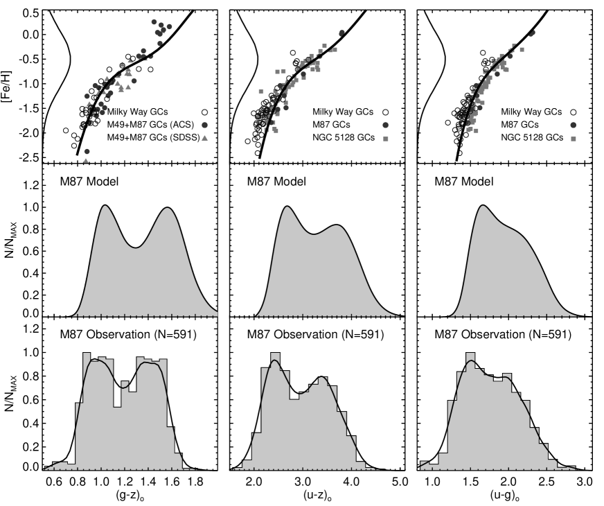
Figure 1: Mutiband ($u$, $g$, and $z$) photometry of GCs in M87 and Monte Carlo simulations for their color distributions. This figure is similar to Figure 2 of Paper II but without color–magnitude diagram panels, and demonstrates how the metallicity–color nonlinearity works. Top row: the observed color–[Fe/H] relations for Galactic GCs with E($B-V$) $<0.3$ (open circles), M49 and M87 GCs with ACS Virgo Cluster Survey photometry (black circles), M49 and M87 GCs with SDSS photometry (gray triangles), and NGC 5128 GCs (gray squares). Solid curves are for the 5th-order polynomial fit to our model data for the GC age of 13.9 Gyr, for which all the morphologies of $g-z$, $u-z$, and $u-g$ color histograms are reproduced simultaneously. The metallicity spread of 10⁶ model GCs is shown along the y-axis, for which a Gaussian normal distribution is assumed ($\langle$[Fe/H]$\rangle$ = $-0.5$ dex and $\sigma$([Fe/H]) = 0.6). Middle row: the left, middle, and right columns represent the color distributions of 10⁶ modeled GCs for the $g-z$, $u-z$, and $u-g$ colors, respectively. Observational uncertainties as a function of luminosity are taken into account in the simulations. Bottom row: the observed color histograms for the M87 GC system. The 591 GCs are used that have reliable measurements in all three bands. Solid lines are smoothed histograms with Gaussian kernels of $\sigma$($g-z$) = 0.05, $\sigma$($u-z$) = 0.15, and $\sigma$($u-g$) = 0.10.

Figure 1, taken from Paper II, demonstrates briefly how this technique works. This specific experiment targeted the M87 GC system, one of the very few early-type galaxies with existing deep $u$-band data. A given metallicity spread (vertical histograms in the top panels) is projected via the theoretical CMRs (solid lines in the top panels) to create the simulated color distributions (gray histograms in the middle panels). For the set of colors shown in the figure, the modeled distributions are noticeably different, especially between $g-z$ (leftmost column) and $u-g$ (rightmost): While the $g-z$ distribution clearly shows a bimodal case with roughly the same heights for the blue and red peaks, the bimodality in the $u-g$ distribution is substantially diminished with the blue peak now dominating the overall distribution. Remarkably, the simulated color distributions are similar to the observed distributions (histograms in the bottom panels), thereby supporting the idea of the nonlinear CMRs. In the same vein, Cantiello & Blakeslee (2007), Kundu & Zepf (2007), Spitler et al. (2008), and Chies-Santos et al. (2011, 2012) highlighted the usefulness of optical–IR colors in constraining the underlying MDFs. More recently, Blakeslee et al. (2012) showed that while the color distribution of GCs in NGC 1399 was clearly bimodal in the optical $g-I$ color, the same bimodality was not present in the optical–IR $I-H$ color. Moreover, the color–color relation between $g-I$ and $I-H$ colors in this galaxy was distinctly nonlinear, indicating significant nonlinearity in the CMR for at least one of these colors.

In this paper, we perform the HST/WFC3 archival $u$-band photometry for the M84 (NGC 4374) GC system and apply the $u$-band technique to the system. M84 is a giant elliptical galaxy located in the Virgo galaxy cluster, and exhibits clear color bimodality in $g-z$ (Peng et al., 2006; Jordán et al., 2009). Section 2 presents our data reduction and photometry procedure and describes the observational data on the GC system of M84. Section 3 gives the result of our simulations and compares it with the observation. The model based on our nonlinear-CMR scenario shows that the $u$-band color distributions are significantly less bimodal than that of $g-z$, and agree well with the observation. Our theoretical prediction for the metallicity distribution of M84 GC system is also presented. Section 4 discusses the implications of our results for the nonlinear-CMR scenario of GC color bimodality (Section 4.1) and for the formation of M84 (Section 4.2) in comparison with M87 (Paper II).

2 THE M84 GLOBULAR CLUSTER SYSTEM: OBSERVATION

2.1 The HST/WFC3 $u$-band Imaging

The first galaxy to which we apply the $u$-band technique proposed by Paper II has been selected by the procedure below. First, we considered galaxies that have been observed as part of the ACS Virgo Cluster Survey (ACSVCS; Côté et al. 2004) and ACS Fornax Cluster Survey (ACSFCS; Jordán et al. 2007). We inspected the $g-z$ color distributions of their GC systems and selected the galaxies showing clear color bimodality. Then, among them, we searched for galaxies with deep HST $u$-band photometry. We identified M84 (NGC 4374), a giant galaxy in the Virgo galaxy cluster, whose GC system exhibits clear bimodality in the ACS $g-z$ distribution and is one of few elliptical galaxies with deep WFC3/UVIS F336W images. The M84 images were observed as part of the science program HST GO-11583 (PI: J. Bregman) to constrain the star formation rate in nearby elliptical galaxies.

Despite the great opportunity that the $u$-band provides, observations of extragalactic GCs in this wavelength are lacking because the atmospheric transmission at $\lambda$ $<$ 4000 Å is limited for ground-based observations (e.g., H. Kim et al., 2013) and because the pre-WFC3 detectors of HST were not efficient (WFPC2: low sensitivity; ACS/HRC: small field size) for systematic studies on extragalactic GCs. Whereas the M87 $u$-band data shown in Figure 1 required 12 orbits of exposure using HST WFPC2 (Paper II), the M84 WFC3 data surpass the WFPC2 data quality with only a fraction of exposure time thanks to the excellent blue sensitivity of WFC3/UVIS. Our M84 result shows that with two orbits of exposure, the $u-g$ color errors become as small as $\sim$ 0.04 mag for a typical GC with $u$ = 25. The M84 fields overlap with the existing ACS/WFC $g$ and $z$ observations in ACSVCS, yet the field of view of WFC3/UVIS is 64 % the size of ACS/WFC. The radial number density profile of GCs in M84 makes $\sim$ 85 % of the ACS/WFC GCs placed in the WFC/UVIS field of view.

2.2 Data Reduction

The data reduction and photometry procedure are outlined as follows. We retrieved two drizzled WFC3 F336W images of M84 from the HST archive. These images are rotated with respect to each other by a position angle of $\sim$ 120 deg while sharing the same image centers. Integration time for each image is 2400 sec. Sources were detected using the daofind task in IRAF and matched with those in the catalog of GC candidates of the ACSVCS (Jordán et al., 2009). Using daophot task in IRAF, aperture photometry was carried out in a 3 pixel radius aperture and adjusted to 10 pixels using empirical aperture corrections derived via several bright and isolated sources in the images. These magnitudes were then corrected to an infinite aperture using the value of $-0.131$ which was derived using the encircled energy fraction provided by the WFC3 Instrument Handbook (Dressel, 2011). Finally, we transformed the magnitudes to the AB system using zero points from Dressel (2011). The corrections for foreground extinction were applied following the same method as in Jordán et al. (2004). The GC candidate catalog of the ACSVCS (Jordán et al., 2009) contains bona fide GCs selected by their magnitudes, $g-z$ colors, and sizes. We further employed color cuts ($g-z$ $<$ 0.5 and $u-g$ $<$ 0.8) to filter out potentially contaminating sources such as background star-forming galaxies.

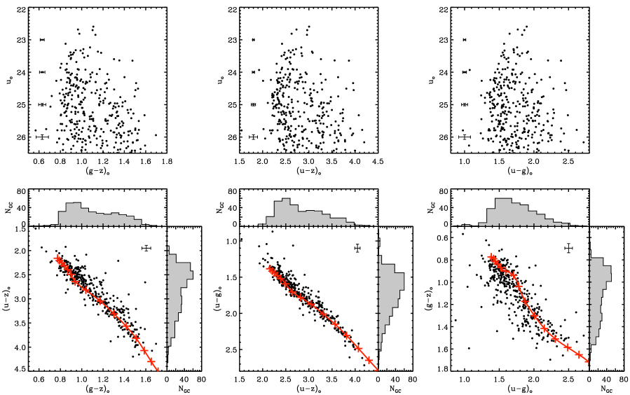
Figure 2: The color–magnitude and color–color diagrams for the observed M84 GCs. This figure is similar to Figure 3 of Paper II, but for M84 GC system (Table 1). Upper row: the observed color–magnitude diagrams. The left, middle, and right panels show the $g-z$, $u-z$, and $u-g$ diagrams, respectively. The $g$ (ABMAG) and $z$ (ABMAG) mags for GC candidates are obtained from the ACSVCS GC catalog (Jordán et al. 2009). The HST/WFC3 archival images are used to measure $u$-band mags (F336W, ABMAG) for the ACSVCS GC catalog. A color cut ($g-z$ $>$ 0.5 and $u-g$ $>$ 0.8) was employed to filter out contaminating sources such as star-forming background galaxies. Black dots in each panel are the selected 362 GCs ($\sigma_{u}$ $<$ 0.2 mag) that have $u$, $g$, and $z$ measurements in common. Lower row: the color–color diagrams and the projected color distributions. Red solid lines represent our model prediction for 13.0-Gyr GCs (Tables 2 and 3) from [Fe/H] = $-2.5$ (top left cross) to +0.5 (bottom right). The red crosses on each model locus mark the uniform [Fe/H] intervals ($\Delta$[Fe/H] = 0.2 dex).

The resultant M84 GCs are presented in Figure 2. Table 1 gives the ID, R.A., Decl., $u$-, $g$-, and $z$-band mags, and their observational errors for M84 GCs. In this study, we consider selected 362 GCs ($\sigma_{u}$ $<$ 0.2 mag) that have reliable $u$, $g$ and $z$ photometry in common, and the sample is $u$-band limited. The top panels of the figure are the color–magnitude diagrams and the bottom panels are the color–color diagrams along with their color distributions shown by gray histograms at the top and side. In the color–magnitude diagrams, the split between two vertical bands of GCs is readily visible for $g-z$, whereas it is less clear for $u-z$ and $u-g$. In the color–color diagrams, the red lines are our theoretical predictions (Tables 2 and 3) for 13-Gyr GCs from the lowest metallicity ([Fe/H] = $-2.5$, top left point) to the highest ([Fe/H] = +0.5, bottom right). The crosses on each model line mark the uniform [Fe/H] intervals of $\Delta$[Fe/H] = 0.2 dex. The larger color spaces at the midpoint of, for example, the $g-z$ versus $u-z$ relation lead to the observed scarcity at the center of the corresponding color distributions.

3 THE M84 GLOBULAR CLUSTER SYSTEM: SIMULATIONS

3.1 Theoretical Color–Metallicity Relations Associated with WFC3 $u_{\rm F336W}$ and ACS $g_{\rm F475W}$ and $z_{\rm F850LP}$

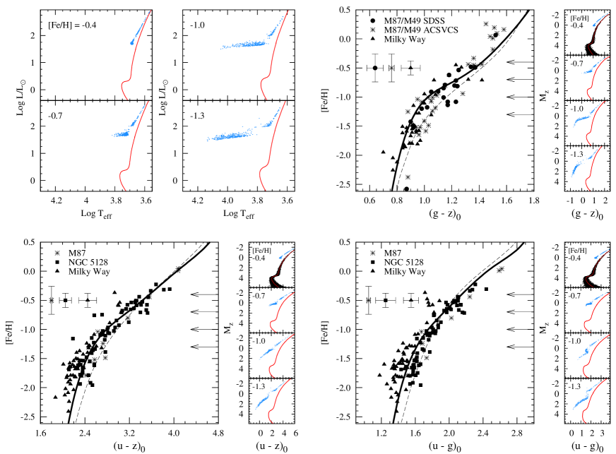
Figure 3: The empirical and theoretical CMRs. This figure is similar to Figure 1 of Paper II, but the $u$-band here is HST/WFC3 $F336W$ (see Figure 4) and the 13-Gyr model is used. Upper left quadrant: synthetic Log $T_{\rm eff}$–Log $L/L_{\sun}$ diagrams of individual stars for 13-Gyr model GCs with various [Fe/H]’s. Red loci are main sequence and giant branch from Yonsei-Yale (Y²) isochrones (Kim et al. 2002), whereas blue dots represent HB stars generated based on the Y² HB tracts (S. Han et al. 2012, in preparation). Upper right quadrant: the ($g-z$)–[Fe/H] CMR. The information on the data are summarized in Table 4. The thick solid line is for the 5th-order polynomial fit to our model data for 13-Gyr GCs, and the dashed line is for the model without inclusion of the HB prescription. Arrows mark the four values of [Fe/H], for which the synthetic color-magnitude diagrams are shown in the small panels on the right. Synthetic color–magnitude diagrams are generated from the synthetic Log $T_{\rm eff}$–Log $L/L_{\sun}$ diagrams (upper left quadrant) using the BaSeL flux library (Westera et al. 2002). The top panel shows individual stars (black and blue dots) with error simulations, whereas the rest panels show only the corresponding isochrones (red loci) and HB stars (blue dots). Lower left quadrant: the same as the upper right quadrant, but for the $u-z$ color. Lower right quadrant: the same as the lower left quadrant, but for the $u-g$ color.

Figure 3 displays the synthetic color–magnitude diagrams for individual stars of the model GCs and the resulting CMRs from the Yonsei Evolutionary Population Synthesis (YEPS) model (Chung et al. 2013). This figure is similar to Figure 1 of Paper II on M87, but specialized for the M84 case. The present model for M84 differs from the Paper II model for M87 in that this study uses the WFC3 $u_{\rm F336W}$ filter (see Figure 4) and the 13-Gyr model GCs. The upper-left quadrant shows the synthetic Log $T_{\rm eff}$ versus Log $L/L_{\sun}$ diagrams, from which the model CMRs for $g-z$, $u-z$, and $u-g$ are generated.

The rest three quadrants of Figure 3 present the theoretical CMRs along with the observations. The upper-right quadrant shows that the $g-z$ CMR is an inverted S-shaped wavy curve, consistent with the observations. The metal-rich ([Fe/H] $\gtrsim$ 0.0) GCs, however, show a $\sim$ 0.1 mag offset in $g-z$ with respect to the theoretical relation. Interestingly, the $g-z$ peak color of red GCs in Figure 1 (and Figure 6 in the next Section 3.2) is redder than the observation by the similar amount. The offset can be explained if metal-rich GCs are slightly younger than blue ones (by $\sim$ 2 Gyr) within the current uncertainty in GC age dating (e.g., Strader et al. 2005) or if they have an extended blue HBs, as observed in the Galactic counterparts (e.g., NGC 6388 and NGC 6441, Rich et al. 1997; Caloi & D’Atona 2007; Yoon et al. 2008). On the other hand, the lower-left and right quadrants show that the CMRs for the $u$-band colors are substantially less inflected than the $g-z$ CMR for the given age, and reproduce the observational data well. To quantify the degree of agreement between the observed data and the theoretical predictions, we obtained the error-weighted $\chi^{2}$ between them: The reduced $\chi^{2}$ values are as low as 0.737, 0.948, and 0.688 for $g-z$, $u-z$, and $u-g$, respectively. It is interesting to notice that the degree of nonlinearity is in order of $g-z$, $u-z$, and $u-g$.

The present model for M84 uses HST/WFC3 $u_{\rm F336W}$ filter for which M84 HST images are available, whereas the M87 model in Paper II was based on HST/WFPC2 $u_{\rm F336W}$. Figure 4 gives the comparison of the sensitivity functions between the WFPC2 $u_{\rm F336W}$ (dashed line) and WFC3 $u_{\rm F336W}$ (solid line) filters on HST. The main peaks of the normalized sensitivity functions at $\lambda$ = 3000 – 4000 Å agree well, yet the WFPC2 $u_{\rm F336W}$ filter used in Paper II shows the red leak at $\lambda$ $\simeq$ 7200 Å. The inset is a zoomed-in plot of $\lambda$ = 6500 – 8000 Å region and highlights the red leak of WFPC2 $u_{\rm F336W}$. We find that the absence of the red leak of WFC3 $u_{\rm F336W}$ used in this study leads to a non-negligible change in $u$-band colors, compared to those based on WFPC2 $u_{\rm F336W}$. Tables 2 and 3 give the model data for $u-z$ and $u-g$ CMRs, respectively, for 10–14 Gyr with fine grid spacing ($\Delta$[Fe/H] = 0.1). The $g-z$ data is identical to, and available from, Table 2 of Paper II.

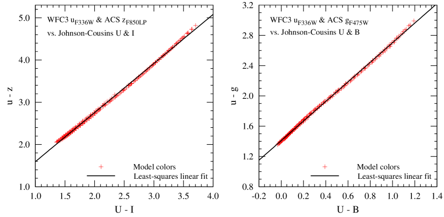
Figure 5: Relationships of $u-z$ versus $U-I$ (left panel) and $u-g$ versus $U-B$ (right). The $u$-band is HST/WFC3 $u_{\rm F336W}$, for which M84 HST images are available. Red crosses represent the model data for synthetic GCs with combinations of age (10 – 15 Gyr of 0.1 Gyr intervals) and [Fe/H] ($-2.5$ – 0.5 dex of 0.1 dex intervals). Least-squares fits (solid lines) to the model data give the two linear equations (see Table 4): ($u-z$) = 1.160 ($U-I$) + 0.434 and ($u-g$) = 1.296 ($U-B$) + 1.412.

We note that, for Milky Way and NGC 5128 GCs in Figure 3, the observational data points of $u-z$ and $u-g$ are obtained by converting currently available $U-I$ and $U-B$, respectively. Figure 5 gives the relationships of $u-z$ versus $U-I$ and $u-g$ versus $U-B$ (solid lines), which are derived from the model data (red crosses) for synthetic GCs with combinations of age (10 – 15 Gyr of 0.1 Gyr intervals) and [Fe/H] ($-$2.5 – 0.5 dex of 0.1 dex intervals). As demonstrated in the figure, $U-I$ and $U-B$ are good proxies to $u-z$ and $u-g$, respectively. As a result, the simple linear fits (solid lines) suffice over the range of ages and metallicities. Also note that, in Figure 3, the data of $u-z$ and $u-g$ for M87 GCs are the WFC3 $u_{\rm F336W}$ colors converted from the WFPC2 $u_{\rm F336W}$ colors. Table 4 summarizes the references to the observed data and the conversion relations used in this study.

3.2 Projection of Metallicities onto Colors

Figure 6 compares the modeled and observed color distributions for M84 GCs. Our working hypothesis is that the CMRs are inflected and create bimodal GC color distributions if the underlying metallicity spread is simply broad as expected from hierarchical merging of numerous (proto-)galaxies. In the simulations, varying ages and mean metallicity produce systematic changes in morphology of $g-z$, $u-z$, and $u-g$ model histograms. With no a priori knowledge on the shape of the underlying MDF, we assume a simple MDF structure of Gaussian normal distribution. The input MDF and age are interactively adjusted until we reach the best match between modeled and observed color histograms for $g-z$, $u-z$ and $u-g$, simultaneously. The combination of parameters that matches up all the morphologies of $g-z$, $u-z$, and $u-g$ histograms at the same time are ($\langle{\rm[Fe/H]}\rangle$, age) = ($-$0.9 dex, 13.0 Gyr) with a fixed $\sigma_{\rm[Fe/H]}$ = 0.6 dex.

To quantify the bimodality properties, we use the Gaussian Mixture Modeling (GMM) code by Muratov & Gnedin (2010). The results of the GMM analysis for the modeled and observed histograms in Figure 6 are given in Table 5, under the two assumptions for a distribution to be homoscedastic (i.e., a mixture of two normal distributions with the same variance) or heteroscedastic (i.e, with different variances). The table gives the mean color ($\mu$), the standard deviation ($\sigma$), and the number fractions ($f$) of blue (subscript $b$) and red (subscript $r$) GCs. The last three columns list the probabilities of preferring a unimodal distribution over a bimodal distribution ($p$-value) derived based on the likelihood ratio test ($\chi^{2}$), on the separation of the means relative to their variances ($DD$) and on the kurtosis of a distribution ($kurt$).

Back in Figure 6, the $g-z$ case is shown in the leftmost column. The column shows how the inflection on a CMR causes color bimodality by projecting equidistant metallicity intervals near the quasi-inflection point (i.e., the most metallicity-sensitive point) onto wider color intervals. In the second row, as an aid to visualizing the simulated color distributions we plot $g-z$ of synthetic GCs against their modeled $u$-band absolute mag, $M_{u}$. Even with the observational uncertainties fully taken into account, the split between two vertical bands of GCs is readily visible. This leads to the dip at the midpoint of the color histogram (third row). In this way, the nonlinear projection results in bimodal color distributions even when the underlying distribution in [Fe/H] is unimodal. The agreement in morphologies between the simulated (third row) and observed (bottom row) $g-z$ distributions is remarkable. A GMM bimodal fitting (Table 5) gives, for the homoscedastic cases, [($\mu_{b}$, $\mu_{r}$), ($f_{b}$, $f_{r}$)] = [(0.98, 1.44), (62 %, 38 %)] for the simulated histogram and [(0.96, 1.35), (63 %, 37 %)] for the observed one. The heteroscedastic case yields [(0.92, 1.34), (44 %, 56 %)] for the simulated histogram and [(0.94, 1.32), (56 %, 44 %)] for the observed one. The result suggests that a color distribution of a GC system does not directly reveal its MDF. But instead, for a given metallicity spread, the color histograms may be primarily determined by the form of the CMR.

The $u-z$ and $u-g$ cases, on the other hand, are shown in the middle and rightmost columns of Figure 6, respectively. It is clear in the bottom panels that the observed $u$-band color distributions are significantly different from the observed $g-z$ distribution: The prominence of bimodality shown in $g-z$ is substantially reduced in $u-z$ and almost diminished in $u-g$. The probabilities of preferring a unimodal distribution over a bimodal distribution derived based on the separation of the means relative to their variances, $p$-value($DD$) = 0.00, 0.07, and 0.42 for $g-z$, $u-z$ and $u-g$ respectively, for the homoscedastic case, and 0.12, 0.45, and 0.61 the heteroscedastic case (Table 5). The third row presents the modeled histograms. The degree of nonlinearity is in order of $g-z$, $u-z$ and $u-g$ (top panels) and, in turn, the strength of color bimodality is in the same order. As a consequence, our model predictions (third row) based on the nonlinear CMR hypothesis match up well with the observed distributions (bottom row) in terms of their overall morphologies.

To be more quantitative, we also apply the GMM test to the simulated and observed histograms for $u-z$ and $u-g$ (Table 5). For the $u-z$ color (middle column), the homoscedastic case gives, [($\mu_{b}$, $\mu_{r}$), ($f_{b}$, $f_{r}$)] = [(2.77, 3.78), (73 %, 27 %)] for the simulated histogram and [(2.57, 3.41), (67 %, 33 %)] for the observed one. The heteroscedastic case yields [(2.55, 3.37), (39 %, 61 %)] for the simulated histogram and [(2.44, 3.08), (36 %, 64 %)] for the observed one. For the $u-g$ color (rightmost column), the homoscedastic case gives [(1.80, 2.45), (86 %, 14 %)] for the simulated histogram and [(1.64, 2.12), (79 %, 21 %)] for the observed one. The heteroscedastic case yields [(1.66, 2.07), (43 %, 57 %)] for the simulated histogram and [(1.52, 1.81), (25 %, 75 %)] for the observed one. We note that the blue peak color of modeled GCs are redder than the observation by $\sim$ 0.1 mag in $u-g$. Our stellar population models show that, for given input parameters, the absolute colors of model GCs can vary up to $\sim$ 0.2 mag in $g-z$, $u-z$ and $u-g$, depending on the choice of stellar evolutionary tracts and model flux libraries. We hence put more weight on the relative color values, i.e., the blue and red GC number fraction and the overall morphologies of the simulated color histograms.

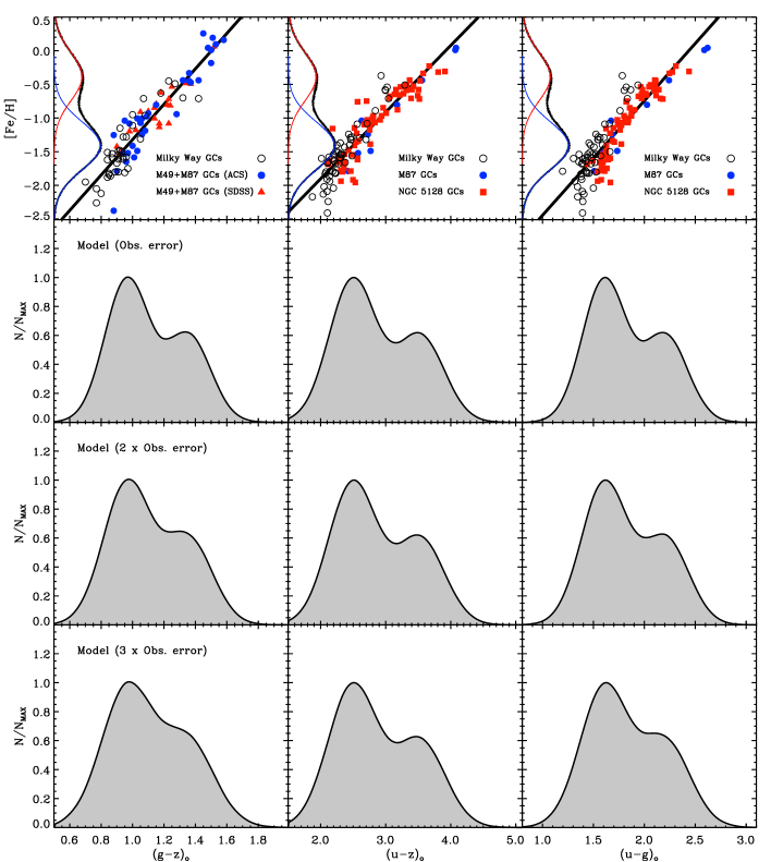
Figure 7: Similar to Figure 6, but the conventional linear CMRs and a combination of two Gaussian distributions are assumed. Top row: the solid lines represent the least-squares fits to the observational data points. The linear equations are [Fe/H] = 2.630 ($g-z$) $-$ 3.950 for $g-z$, [Fe/H] = 0.990 ($u-z$) $-$ 3.882 for $u-z$, and [Fe/H] = 1.702 ($u-g$) $-$ 4.146 for $u-g$. The metallicity distribution of 10⁶ model GCs is shown along the y-axis, for which two Gaussian normal distributions are adapted from Figure 8 (dotted line in the bottom-left panel). The mean [Fe/H] and its dispersion, and the number fraction, ($\langle$[Fe/H]$\rangle$, $\sigma$([Fe/H]), $f$), are ($-$1.41 dex, 0.36 dex, 62 %) for the metal-poor group (blue lines) and ($-$0.39 dex, 0.36 dex, 38 %) for the metal-rich group (red lines). The sum of the two distributions is given by the black line. Second row: Monte Carlo simulations for the color distributions. The left, middle, and right columns represent the color distributions of 10⁶ modeled GCs for the $g-z$, $u-z$, and $u-g$ colors, respectively. The color scatter just as given by the observational uncertainties in color (Table 6) is used. Third and bottom rows: the same as the second row, but twice and three times larger scatters than the observational uncertainties are used.

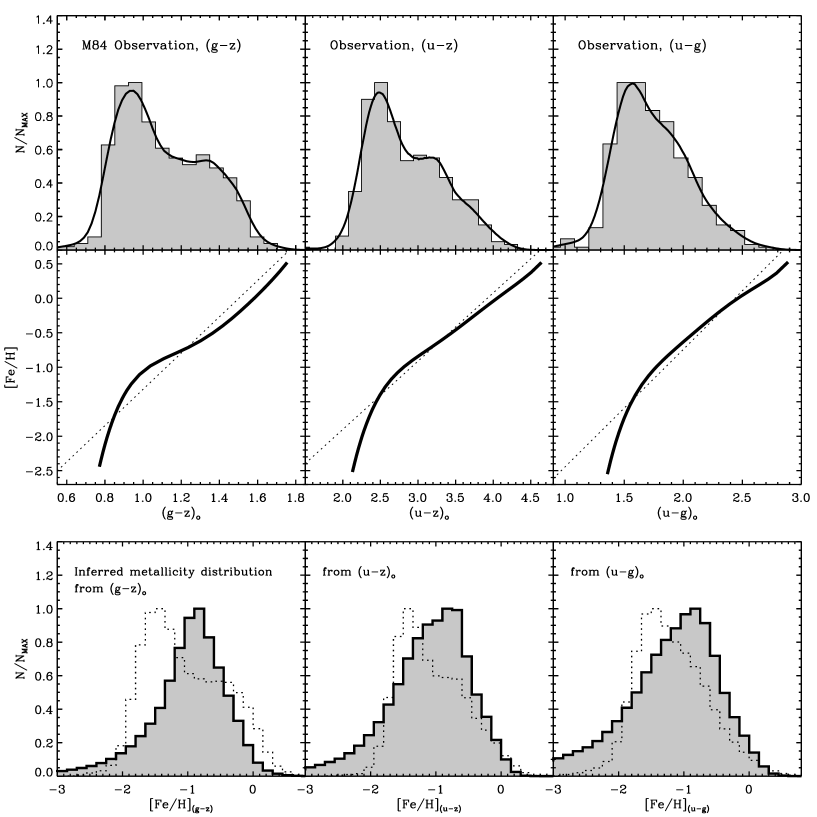
Figure 8: The observed $g-z$, $u-z$, and $u-g$ color distributions and their inferred MDFs for the GC system of M84. Top row: the same as the bottom row of Figure 6. Middle row: the same as the top row of Figure 6, but the dotted lines represent the least-squares fits to the observational data points that are not shown here for clarity (see Figure 7). Bottom row: the left, middle, and right panels show the [Fe/H]_(g-z), [Fe/H]_(u-z), and [Fe/H]_(u-g) distributions obtained independently from the $g-z$, $u-z$, and $u-g$ color distributions, respectively. The MDFs are derived from the smoothed histograms in the top row via the nonlinear color-to-metallicity transformations (gray histograms with solid lines) and via the linear transformation (open histograms with dotted lines).

The metallicity–color nonlinearity provides a good explanation for the systematic variation in strength of color bimodality of M84 GC system (Figure 6). Nevertheless, it is still important to check whether observational measurement errors and possible GC-to-GC variations in the physical parameters play any role in weakening bimodality of $u$-band colors. Figure 7 demonstrates how a bimodal [Fe/H] distribution behaves in the color domain as the color scatter substantially increases to a factor of three. In the first row, we assume the conventional linear CMRs and a bimodal underlying MDF. The combination of two Gaussian normal distributions is adapted from the [Fe/H]_(g-z) histogram in Figure 8 (dotted histogram in the bottom-left panel). The second row allows the color scatter just as given by the observational uncertainties in color. The measurement errors of $g-z$, $u-z$ and $u-g$ for each magnitude bin and the entire sample are summarized in Table 6. For the entire 362 GCs, the median $u-z$ and $u-g$ errors are respectively 0.058 and 0.056 mag, which are both $\sim$1.4 times larger than 0.041 mag for $g-z$. However, the approximate color ranges spanned by $g-z$, $u-z$, and $u-g$ distributions are 0.6 $\sim$ 1.7 mag, 1.9 $\sim$ 4.3 mag, and 1.0 $\sim$ 2.7 mag, respectively. That is, [$\Delta$($g-z$), $\Delta$($u-z$), $\Delta$($u-g$)] $\simeq$ [1.1, 2.4, 1.7], meaning that the baselines of $u-z$ and $u-g$ are respectively 2.2 and 1.5 times longer than that of $g-z$. As a result, the relative sizes ($\epsilon$) of error bars are calculated to be [$\epsilon$($g-z$) : $\epsilon$($u-z$) : $\epsilon$($u-g$)] $\simeq$ [1.0 / 1.1 : 1.4 / 2.4 : 1.4 / 1.7] $\simeq$ [0.9 : 0.6 : 0.8]. It is important to observe that in a relative sense, the observational uncertainties in three colors are quite comparable with one another and in fact the errors in $u-z$ and $u-g$ are smaller than that in $g-z$. This is evident in the error bars shown in Figure 3 as well. As a consequence, the modeled $u-z$ and $u-g$ histograms (middle and right columns in the second row of Figure 7) based on the conventional linear CMRs are not consistent with the observations (Figure 6). It is, therefore, highly unlikely that bimodal histograms are simply blurred by larger observational errors in the $u$-band.

In Figure 7, we also test how extra color uncertainty posed by the GC-to-GC variations in terms of the stellar population parameters (e.g., age, [$\alpha$/Fe], helium abundance, initial mass function, and multiple stellar populations) exerts effect on the color distributions. Adopting a single relation between metallicities and colors should underrate the possible spread of color distributions, and the intrinsic scatter around the [Fe/H]–color calibrations could be a contributor to diluting [Fe/H] distributions in color space. In order to accommodate such variations, the third and bottom rows allow twice and three times larger scatter than the observational uncertainties. Although the actual GC-to-GC variations of M84 GC system in physical parameters are not known, the color–color diagrams in Figure 2 give an indication that extra scatter other than measurement errors around the relations is fairly small. Our experiment shows that 1.2 times the measurement error best reproduce the $g-z$ vs. $u-z$ and the $u-z$ vs. $u-g$ diagrams and that 1.4 times match the $u-g$ vs. $g-z$ diagram. So, twice and three times larger scatter in the third and bottom rows of Figure 7 are well beyond the estimates of GC-to-GC variations of M84 GCs. Even with the excessively large scatter in color, the way a bimodal metallicity distribution manifest itself in color are not consistent with the observation (Figure 6). One might argue that the difference in the overall slopes, $\Delta$color/$\Delta$[Fe/H], of the linear fits, combined with scatters in color, could lead to varying degrees of color bimodality for a bimodal [Fe/H] distribution. However, the apparent slopes are turned out to be almost identical (first row) because the different $\Delta$color/$\Delta$[Fe/H] slopes are fully compensated by the the differing color baselines ranged by $g-z$, $u-z$, and $u-g$ distributions, i.e., [$\Delta$($g-z$), $\Delta$($u-z$), $\Delta$($u-g$)] $\simeq$ [1.1, 2.4, 1.7]. Therefore, it is highly unlikely that, for M84 GC system, blurring due to the GC-to-GC scatter smears out a bimodal MDF in the color domain.

We finish this Section by emphasizing that in the context of the nonlinear CMRs, the systematic variation in the histogram morphology for different colors is readily explained if the shape of the CMRs is subject to colors (Figure 6). By contrast, in the conventional view established based on the linear CMRs, the color histogram morphology has no reason to vary depending on the colors, unless the scatter are significantly different color-by-color. That is, two distinct GC subpopulations should manifest themselves more or less in the same way even in different color distributions (Figure 7). We therefore conclude for M84 GC system that not only it is unnecessary to assume a bimodal [Fe/H], but also it is more appropriate to assume a unimodal [Fe/H].

3.3 De-projection of Colors onto Metallicities

In an attempt to investigate the possibility of using the theoretical CMRs as a tool for recovering the MDFs, this Section performs the de-projection of the observed color distributions of M84 GCs. The metallicity-to-color projection carried out in Section 3.2 should be reversible, but the inverse transformation can be negatively affected by the following two factors. First, compared to the metallicity-to-color transformation, the inverse transformation is more susceptible to the incompleteness of current population synthesis models. As mentioned in Section 3.2, the different choice of stellar evolutionary tracks and model flux libraries can result in up to $\sim$ 0.2 mag variation in $g-z$, $u-z$, and $u-g$ for given input parameters. Supposing that a CMR is erroneously shifted in the color direction, the metallicity-to-color conversion would still give correct color histogram morphologies, yet the inverse conversion would yield incorrect MDFs. Second, the color-to-metallicity de-projections can also be hampered by the color uncertainty due to the observational measurement errors and the intrinsic GC-to-GC variations. Obviously, the uncertainty makes the histograms of colors broader than the intrinsic distributions and thus leads to the inferred MDFs that are broader than the true MDFs. This effect, when combined with the steepness of the metal-poor part of the nonlinear CMRs, can result in the enhanced frequency of GCs at the very metal-poor tails ([Fe/H] $<$ $-2.5$). Thus, the exact shape of the metal-poor wings of inferred MDFs should be viewed with caution. Nevertheless, careful comparison of the GC MDFs obtained independently from various color histograms will shed light on the color–metallicity nonlinearity issue.

Figure 8 shows the inferred MDFs as products of de-projection of the observed colors onto metallicities, using both nonlinear and linear CMRs. The top row is identical to the bottom row of Figure 6, showing the observed $g-z$, $u-z$ and $u-g$ distributions. The bottom row presents the GC metallicity histograms obtained independently from the $g-z$, $u-z$ and $u-g$ colors based on the theoretical CMRs shown in the middle row. The best-fit age (13 Gyr) for M84 GCs derived in Figure 6 is also used here. The observed color histograms with different morphologies (top row) are all converted to the MDFs (filled histograms in the bottom row) that have a strong metal-rich peak with a wing on the metal-poor side. Although the inverse conversion inevitably overestimates the metal-poor tail of inferred MDFs, the three inferred metallicity histograms are consistent with one another in terms of their overall shape and peak metallicities at [Fe/H] $\simeq$ $-0.9$. By contrast, the distributions (dotted histograms in the bottom row) derived based on the conventional linear color–metallicity relations (dotted lines in the middle row) do not agree with one another. We emphasize that under the nonlinear-CMR assumption, the model invariably obtains very similar morphologies and peak positions of the MDFs from different colors, strongly indicating that the color–metallicity nonlinearity is real.

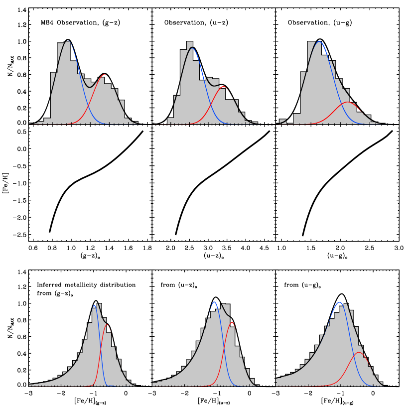
Figure 9: The observed $g-z$, $u-z$, and $u-g$ color distributions and their inferred MDFs for the GC system of M84. This figure is the same as Figure 8, but the observed histograms are expressed by a sum of two (i.e., blue and red) Gaussian distributions. Top row: the result of the GMM analysis. The homoscedastic (same variance) case are used for the GMM test. The blue, red, and black lines represent the blue, red, and total GCs, with the peak colors and number fractions of blue and red GCs being [(0.96, 1.35), (63 %, 37 %)] for $g-z$, [(2.56, 3.41), (66 %, 34 %)] for $u-z$, and [(1.63, 2.12), (78 %, 22 %)] for $u-g$, respectively. Middle row: the same as the middle row of Figure 8. Bottom row: the same as the bottom row of Figure 8, but the black, blue, and red lines are respectively obtained from the corresponding curves in the top row via the nonlinear color-to-metallicity transformations in the middle row.

Figure 9 presents the same de-projection experiment as in Figure 8 with the identical observational data, but here the observed color histograms (top row) are broken into two hypothetical subgroups following the conventional notion. The distributions of blue and red GCs are fit with a pair of Gaussian functions. A GMM bimodal fitting (Table 5) gives the mean colors and the number fractions of the blue and red subpopulations as [($\mu_{b}$, $\mu_{r}$), ($f_{b}$, $f_{r}$)] = [(0.96, 1.35), (63 %, 37 %)] for $g-z$, [(2.57, 3.41), (67 %, 33 %)] for $u-z$, and [(1.64, 2.12), (79 %, 21 %)] for $u-g$. We use the GMM analysis for the same variance case, but the use of different variances does not affect our conclusion. The two Gaussian functions and their sums in the top row are converted to MDFs through the nonlinear color-to-metallicity conversions in the middle row. In the bottom row, the black, blue and red histograms are respectively obtained from the corresponding curves in the top row. Under the nonlinear-CMR assumption, the three color distributions with dissimilar blue-to-red GC ratios are all transformed into simple, broad MDFs with the similar morphologies. The broad MDF of the M84 GC system is in accordance with the hierarchical merging paradigm of galaxy formation, and two hypothetical subgroups are not necessarily required. Therefore, the test performed in Figure 9 gives further support for the nonlinear-CMR scenario for the color bimodality.

4 DISCUSSION

We have presented archival HST/WFC3 F336W ($u$-band) photometry of the GC system in M84, against which our simulated GC color distributions are compared. The agreement between the observation and simulations strengthens the view that the metallicity–color nonlinearity effect has a key role in producing color bimodality.

This Section discusses the implications regarding the nonlinear-CMR scenario for GC color bimodality (Section 4.1) and elliptical galaxy formation theories (Section 4.2). Here we combine the result on M84 with that of M87 presented in Paper II to carry out a comparative examination of their GC systems. M87 and M84 represent galaxies situated in a cluster of galaxies, and M87, compared to M84, is an example of a more massive galaxy closer to the heavily populated inner core of a galaxy cluster. Note that the GC samples for M87 (with HST ACS/WFC and WFPC2) and M84 (with HST ACS/WFC and WFC3) are confined to $R\lesssim R_{\rm eff}$ at the Virgo distance ($\simeq$ 16.5 Mpc).

4.1 Globular Cluster Systems of M87 and M84 as Testbeds of the Metallicity–Color Nonlinearity Scenario

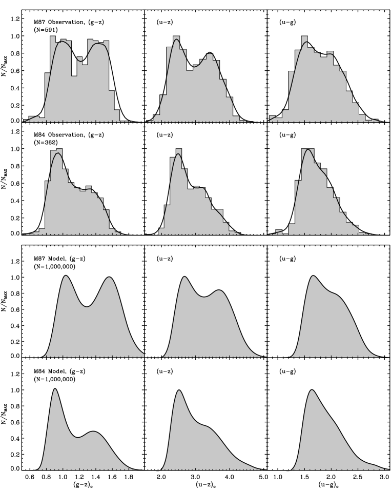
Figure 10: Comparison between the observed and simulated color distributions of M87 (Paper II) and M84 (this study) GC systems. The histograms are identical to the ones already shown in Figures 1 (for M87) and 6 (for M84). Upper six panels: the observed $g-z$, $u-z$, and $u-g$ color distributions for M87 and M84 GCs. Note that $u$ corresponds HST/WFPC2 $F336W$ for M87 and HST/WFC3 $F336W$ for M84. Lower six panels: the simulated $g-z$, $u-z$, and $u-g$ color distributions for M87 and M84 GCs. The best-fit parameters for M87 and M84 are listed in Table 8.

There is extensive ongoing debate as to, between the metallicity difference and the nonlinear projection effect, which plays the more important role in making GC color bimodality. To address this issue, Figure 10 presents the observed and simulated color distributions of M87 (Paper II) and M84 (this study) GC systems. The upper six panels compare the observed histograms for the $g-z$, $u-z$, and $u-g$ colors of M87 (upper row) and M84 (lower row) GCs. Both galaxies show that bimodality in the $g-z$ distribution (leftmost panels) is reduced in $u-z$ (middle) and further weakened in $u-g$ (rightmost), in a very systematic manner. When one compares the two galaxies in the given colors, the red peak of M84 is significantly weaker than that of M87 for every color histogram, again, in a very systematic way.

The lower six panels show that the orderly behavior of the observed color distributions is reproduced well by the simulated histograms from $g-z$ to $u-z$ to $u-g$ for a given galaxy and from M87 to M84 for a given color. The best-fit parameters for M87 and M84 are summarized in Table 8, along with their basic observational information. As described in Section 3.2, the model needs only two adjusting parameters, i.e., the mean [Fe/H] ($\langle$[Fe/H]$\rangle$) with a fixed $\sigma_{\rm[Fe/H]}$ and age ($t$). The parameters are selected to be ($\langle$[Fe/H]$\rangle$, $t$) = ($-0.5$ dex, 13.9 Gyr) and ($-0.9$ dex, 13.0 Gyr) for the M87 and M84 GC systems, respectively.

The fact that all the simulations in Figure 10 are performed under the assumption of the unimodal [Fe/H] spread greatly reduces the conventional demand for the two GC subgroups to explain the color bimodality. It is therefore suggested that the nonlinear CMRs are truly universal for old GC systems. Interestingly, although hampered by the possible presence of young GC populations ($\ll$ 10 Gyr), there are some GC systems showing bimodal spectroscopic metallicity (e.g., NGC 3115 (S0 type) in Brodie et al. 2012 and Usher et al. 2012, but see also Paper V). In such systems, the inflected CMRs often create stronger bimodality in the color domain.

The results on the GC systems of the two giant galaxies in the Virgo galaxy cluster lend confidence to the effectiveness of the “$u$-band” technique to potentially judge whether the true form of CMRs are linear or nonlinear. In this regard, the HST/WFC3 observations in F336W for nearby large elliptical galaxies are highly anticipated. If the nonlinearity of CMRs is found to be favored by the future observations, it will change much of the current thought on the GC color bimodality as well as the formation of GCs and their host galaxies.

4.2 Globular Cluster Systems of M87 and M84 as Tracers of Formation of their Host Galaxies

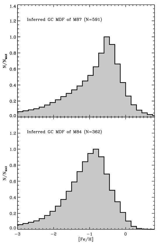
Figure 11: Comparison between inferred GC MDFs of M87 (Paper II) and M84 (this study). Each MDF is an average of the [Fe/H]_(g-z), [Fe/H]_(u-z), and [Fe/H]_(u-g) histograms (Figure 8) that are derived respectively from the $g-z$, $u-z$, and $u-g$ color distributions via the nonlinear color-to-[Fe/H] conversions.

Clusters can place important constraints on the histories of chemical enrichment and star formation of their parent galaxies. Figure 11 presents the inferred MDFs of M87 (Paper II) and M84 (this study) GC systems. As described in Section 3.3, the distributions of [Fe/H]_(g-z), [Fe/H]_(u-z), and [Fe/H]_(u-g) were independently derived respectively from the $g-z$, $u-z$, and $u-g$ histograms via the nonlinear color-to-[Fe/H] de-projection. Each [Fe/H] distribution is an average of the three histograms of [Fe/H]_(g-z), [Fe/H]_(u-z) and [Fe/H]_(u-g) for each galaxy. Despite the clear difference in the observed GC color histograms between M87 and M84 (Figure 10), the nonlinear inverse conversions result in the similar MDF shapes, which are characterized by a sharp metal-rich peak with a metal-poor wing.

Recently, Paper III demonstrated that the strongly-peaked, unimodal MDFs with broad metal-poor tails are similar to the MDFs of resolved halo stars in nearby elliptical galaxies, e.g., the M87 field-star MDF reported by Bird et al. (2010). The characteristic form of the MDFs of both GCs and field stars may have a profound implication because the unimodal, skewed MDFs are products of rather continuous chemical evolution. The strongly peaked GC MDFs are consistent with hierarchical formation theories of giant elliptical galaxies, in which an aggregate of a large number of protogalactic gas clouds forms stars and GCs on a relatively short timescale. Furthermore, the mutual similarity in the MDF shape between M87 and M84 GC systems (Figure 10) suggests a common process of GC formation and evolution between the two systems.

It is interesting that while the two MDFs have similar shape, they have differing peak positions at [Fe/H]_peak = $-0.5$ and $-0.9$ for M87 and M84, respectively. That the M87 GC MDF is more metal-rich than the M84 GC MDF implies that the chemical enrichment in M87 is more processed than that in M84. Another difference between the two GC systems lies in their inferred ages, in the sense that M87 appears older than M84 by $\sim$ 1 Gyr (see Paper III for a detailed discussion of the systematic age difference among GC systems). The possible age difference may be reminiscent of the galaxy downsizing paradigm whereby stars of dimmer galaxies, on average, formed later than those of brighter galaxies. This notion seems to hold for GC systems as well. That is, GC systems in fainter galaxies are on average younger, which was referred to as “downsizing of GC systems” in Paper III.

Combining the MDF and age arguments above together, we paint a picture in which M87 as a more massive galaxy in a denser environment had earlier GC formation and more efficient chemical enrichment than M84. We therefore propose a scenario that the formation and metal enrichment of GCs have started earlier and proceeded more efficiently in more massive galaxies in denser environments (see Paper III for more details). In this view, the most metal-poor GCs in most massive galaxies in galaxy clusters may serve as the first generation of GCs in the universe.

Figure 4: Comparison of normalized sensitivity between the WFPC2 $u_{\rm F336W}$ filter (dashed line, Paper II) and WFC3 $u_{\rm F336W}$ filter (solid line, this study) on HST. The inset is a zoomed-in plot of the red leak of the WFPC2 $u_{\rm F336W}$ filter at $\lambda$ = 6700 – 7800 Å. The absence of the red leak of WFC3 $u_{\rm F336W}$ leads to a non-negligible change in $u$-band colors such as $u-z$ and $u-g$, compared to WFPC2 $u_{\rm F336W}$.

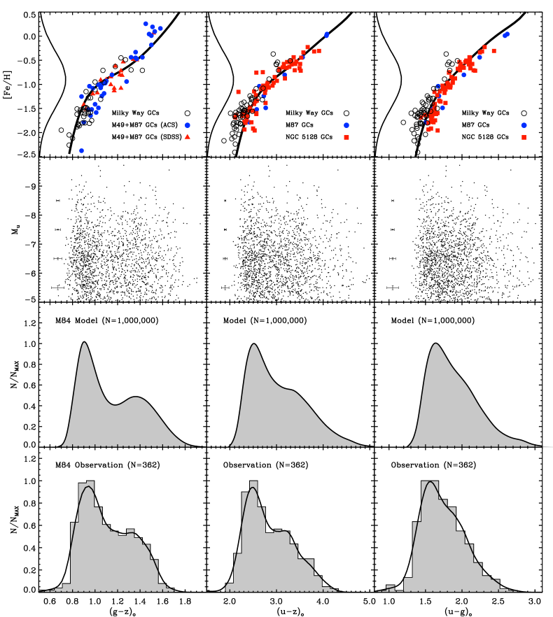
Figure 6: Mutiband ($u$, $g$, and $z$) observation of GCs in M84 and Monte Carlo simulations for their color distributions. Top row: the same as the CMRs in Figure 2. The metallicity spread of 10⁶ model GCs is shown along the y-axis, for which a Gaussian normal distribution is assumed. The best-fit metallicity and age to reproduce the morphologies of $g-z$, $u-z$, and $u-g$ color histograms simultaneously is $\langle$[Fe/H]$\rangle$ = $-0.9$ with $\sigma$([Fe/H]) = 0.6 and 13.0 Gyr, respectively. Second row: the left, middle, and right columns represent the color–magnitude diagrams of 2000 randomly selected model GCs for the $g-z$, $u-z$, and $u-g$ colors, respectively. The colors are transformed from [Fe/H]’s by using the theoretical relation shown in the top row. For the integrated $u$-band absolute mag, $M_{u}$, a Gaussian luminosity distribution ($\langle$$u$$\rangle$ = 25.2, $\sigma$($u$) = 1.15, and distance modulus ($u-M_{u}$) = 31.33) is assumed according to the observation. Observational uncertainties as a function of $M_{u}$ shown by error bars are obtained from the actual observations (Table 6) and taken into account in the simulations. Third row: the left, middle, and right columns represent the color distributions of 10⁶ modeled GCs for the $g-z$, $u-z$, and $u-g$ colors, respectively. Bottom row: the same as the third row, but the observed color histograms for the M84 GC system. The 362 GCs were used that have $u$, $g$, and $z$ measurements in common. Solid lines are smoothed histograms with Gaussian kernels of $\sigma$($g-z$) = 0.06, $\sigma$($u-z$) = 0.14, and $\sigma$($u-g$) = 0.10, respectively.

Table 1: The $u$-, $g$-, and $z$-band Mags and their Observational Errors for the M84 GC Candidates

GC ID	RA (J2000)	DEC (J2000)	$u_{0}$	$u$ Error	$g_{0}$	$g$ Error	$z_{0}\tablenotemark{a}$	$z$ Error
			(WFC3 $F336W$)		(ACS/WFC $F475W$)		(ACS/WFC $F850LP$)
1	186.2654720	12.8857011	23.905	0.047	22.428	0.032	21.259	0.037
2	186.2642216	12.8872940	23.416	0.030	21.586	0.023	20.576	0.021
3	186.2640406	12.8867801	23.932	0.043	22.858	0.014	22.009	0.071
4	186.2666970	12.8860645	25.679	0.280	23.420	0.064	21.750	0.033
5	186.2637346	12.8868181	25.054	0.119	23.211	0.030	21.830	0.031
6	186.2644810	12.8854047	26.143	0.205	24.772	0.125	22.918	0.107
7	186.2635033	12.8870891	24.908	0.067	23.006	0.027	21.831	0.047
8	186.2670468	12.8884144	24.947	0.057	23.653	0.051	22.835	0.051
9	186.2675672	12.8860944	24.496	0.041	22.851	0.035	21.614	0.041
10	186.2660015	12.8845349	24.778	0.043	23.410	0.029	22.569	0.099
$\cdots$	$\cdots$	$\cdots$	$\cdots$	$\cdots$	$\cdots$	$\cdots$	$\cdots$	$\cdots$
$\cdots$	$\cdots$	$\cdots$	$\cdots$	$\cdots$	$\cdots$	$\cdots$	$\cdots$	$\cdots$
$\cdots$	$\cdots$	$\cdots$	$\cdots$	$\cdots$	$\cdots$	$\cdots$	$\cdots$	$\cdots$

Table 2: Theoretical $u-z$ for Synthetic GCs with Various Ages ($t$) Based on the YEPS Model without ($w/o$) and with ($w$) the Inclusion of the HB Prescription (The 5th-order Polynomial Fits to the Model Data).

[Fe/H]	$u-z$ ($u$ = WFC3/$F336W$, $z$ = ACS/WFC/$F850LP$)
	t = 10.0 (Gyr)		10.5		11.0		11.5		12.0		12.5		13.0		13.5		14.0
	$w/o$	$w$	$w/o$	$w$	$w/o$	$w$	$w/o$	$w$	$w/o$	$w$	$w/o$	$w$	$w/o$	$w$	$w/o$	$w$	$w/o$	$w$
–2.5	2.171	2.078	2.189	2.078	2.208	2.078	2.224	2.086	2.240	2.093	2.254	2.112	2.268	2.132	2.280	2.155	2.293	2.178
–2.4	2.194	2.104	2.213	2.104	2.232	2.104	2.249	2.110	2.266	2.116	2.281	2.135	2.296	2.154	2.310	2.178	2.324	2.202
–2.3	2.220	2.132	2.239	2.133	2.259	2.133	2.276	2.137	2.294	2.140	2.310	2.159	2.326	2.178	2.341	2.203	2.356	2.228
–2.2	2.247	2.163	2.267	2.163	2.287	2.163	2.305	2.165	2.323	2.166	2.340	2.185	2.357	2.203	2.373	2.229	2.390	2.255
–2.1	2.275	2.195	2.296	2.195	2.317	2.196	2.336	2.195	2.355	2.194	2.373	2.212	2.391	2.229	2.408	2.256	2.426	2.284
–2.0	2.307	2.230	2.328	2.230	2.349	2.231	2.369	2.228	2.389	2.225	2.408	2.241	2.427	2.257	2.445	2.286	2.463	2.314
–1.9	2.341	2.268	2.363	2.268	2.385	2.269	2.405	2.263	2.426	2.258	2.446	2.274	2.465	2.288	2.485	2.318	2.504	2.346
–1.8	2.377	2.309	2.400	2.310	2.423	2.310	2.445	2.302	2.466	2.295	2.486	2.309	2.507	2.322	2.527	2.351	2.546	2.380
–1.7	2.417	2.355	2.441	2.355	2.465	2.356	2.487	2.345	2.509	2.335	2.531	2.347	2.552	2.358	2.572	2.388	2.592	2.416
–1.6	2.461	2.405	2.486	2.405	2.511	2.406	2.534	2.393	2.557	2.380	2.579	2.390	2.600	2.399	2.620	2.428	2.641	2.455
–1.5	2.510	2.460	2.536	2.461	2.561	2.462	2.585	2.446	2.609	2.431	2.631	2.438	2.653	2.444	2.673	2.472	2.693	2.498
–1.4	2.563	2.521	2.590	2.522	2.617	2.524	2.642	2.507	2.666	2.491	2.688	2.493	2.710	2.496	2.730	2.521	2.750	2.543
–1.3	2.623	2.588	2.651	2.591	2.679	2.593	2.704	2.577	2.729	2.560	2.751	2.557	2.773	2.556	2.792	2.575	2.811	2.594
–1.2	2.687	2.662	2.717	2.666	2.747	2.670	2.773	2.656	2.799	2.640	2.820	2.632	2.842	2.626	2.860	2.638	2.877	2.651
–1.1	2.757	2.741	2.789	2.748	2.820	2.755	2.847	2.746	2.874	2.734	2.895	2.721	2.917	2.709	2.933	2.710	2.949	2.714
–1.0	2.832	2.825	2.866	2.836	2.899	2.847	2.927	2.845	2.955	2.842	2.976	2.824	2.998	2.808	3.013	2.794	3.028	2.787
–0.9	2.911	2.913	2.946	2.929	2.981	2.945	3.011	2.951	3.040	2.958	3.062	2.942	3.085	2.925	3.099	2.894	3.113	2.873
–0.8	2.992	3.004	3.030	3.025	3.067	3.045	3.098	3.060	3.129	3.077	3.153	3.067	3.176	3.056	3.191	3.012	3.205	2.974
–0.7	3.076	3.096	3.115	3.122	3.154	3.148	3.187	3.169	3.221	3.192	3.247	3.192	3.273	3.191	3.289	3.147	3.305	3.098
–0.6	3.161	3.190	3.202	3.220	3.242	3.251	3.278	3.277	3.314	3.305	3.343	3.314	3.372	3.323	3.391	3.293	3.410	3.249
–0.5	3.248	3.286	3.290	3.320	3.332	3.354	3.370	3.384	3.408	3.414	3.441	3.432	3.473	3.450	3.498	3.441	3.522	3.418
–0.4	3.337	3.383	3.380	3.421	3.423	3.458	3.463	3.490	3.504	3.521	3.540	3.547	3.577	3.573	3.607	3.584	3.638	3.591
–0.3	3.429	3.484	3.472	3.524	3.515	3.563	3.558	3.596	3.600	3.628	3.641	3.660	3.681	3.692	3.719	3.721	3.756	3.753
–0.2	3.525	3.590	3.568	3.631	3.611	3.670	3.655	3.704	3.699	3.737	3.743	3.774	3.788	3.810	3.831	3.853	3.876	3.901
–0.1	3.627	3.703	3.669	3.742	3.711	3.781	3.756	3.816	3.800	3.850	3.848	3.890	3.895	3.930	3.945	3.981	3.995	4.036
0.0	3.735	3.821	3.775	3.858	3.815	3.895	3.860	3.932	3.905	3.967	3.954	4.010	4.004	4.052	4.058	4.105	4.113	4.161
0.1	3.848	3.945	3.885	3.978	3.923	4.012	3.967	4.051	4.011	4.089	4.062	4.133	4.113	4.176	4.171	4.228	4.229	4.279
0.2	3.960	4.068	3.997	4.099	4.033	4.131	4.076	4.172	4.120	4.214	4.171	4.257	4.222	4.301	4.281	4.348	4.340	4.394
0.3	4.064	4.180	4.102	4.213	4.139	4.246	4.183	4.289	4.226	4.332	4.277	4.376	4.328	4.420	4.388	4.465	4.447	4.507
0.4	4.154	4.277	4.195	4.315	4.236	4.352	4.281	4.394	4.326	4.436	4.378	4.482	4.430	4.527	4.488	4.576	4.547	4.623
0.5	4.229	4.358	4.275	4.402	4.321	4.447	4.370	4.487	4.419	4.526	4.472	4.575	4.525	4.623	4.584	4.681	4.643	4.743

Table 3: Theoretical $u-g$ for Synthetic GCs with Various Ages ($t$) Based on the YEPS Model without ($w/o$) and with ($w$) the Inclusion of the HB Prescription (The 5th-order Polynomial Fits to the Model Data).

[Fe/H]	$u-g$ ($u$ = WFC3/$F336W$, $g$ = ACS/WFC/$F475W$)
	t = 10.0 (Gyr)		10.5		11.0		11.5		12.0		12.5		13.0		13.5		14.0
	$w/o$	$w$	$w/o$	$w$	$w/o$	$w$	$w/o$	$w$	$w/o$	$w$	$w/o$	$w$	$w/o$	$w$	$w/o$	$w$	$w/o$	$w$
–2.5	1.437	1.439	1.441	1.420	1.444	1.398	1.448	1.380	1.452	1.361	1.456	1.363	1.460	1.364	1.465	1.374	1.469	1.384
–2.4	1.452	1.452	1.456	1.436	1.461	1.420	1.465	1.400	1.470	1.380	1.475	1.380	1.480	1.379	1.485	1.388	1.491	1.398
–2.3	1.467	1.465	1.472	1.453	1.478	1.442	1.483	1.421	1.488	1.400	1.494	1.397	1.500	1.394	1.506	1.403	1.513	1.412
–2.2	1.483	1.479	1.489	1.471	1.495	1.464	1.501	1.443	1.507	1.421	1.514	1.415	1.521	1.410	1.528	1.419	1.535	1.428
–2.1	1.500	1.494	1.506	1.490	1.513	1.487	1.520	1.465	1.527	1.443	1.535	1.434	1.542	1.427	1.549	1.435	1.557	1.444
–2.0	1.517	1.511	1.525	1.509	1.532	1.509	1.540	1.488	1.548	1.466	1.556	1.455	1.564	1.445	1.572	1.453	1.580	1.461
–1.9	1.535	1.528	1.544	1.530	1.552	1.533	1.561	1.512	1.569	1.490	1.578	1.477	1.586	1.465	1.595	1.472	1.603	1.479
–1.8	1.554	1.547	1.564	1.551	1.573	1.557	1.582	1.537	1.592	1.516	1.601	1.501	1.610	1.486	1.618	1.493	1.627	1.498
–1.7	1.574	1.567	1.585	1.574	1.595	1.581	1.605	1.563	1.615	1.543	1.625	1.527	1.634	1.510	1.643	1.515	1.652	1.519
–1.6	1.595	1.589	1.607	1.598	1.618	1.607	1.629	1.590	1.639	1.572	1.649	1.554	1.659	1.535	1.668	1.539	1.677	1.541
–1.5	1.617	1.613	1.630	1.624	1.642	1.633	1.653	1.619	1.665	1.604	1.675	1.585	1.685	1.564	1.694	1.565	1.703	1.565
–1.4	1.641	1.639	1.654	1.651	1.667	1.660	1.679	1.649	1.691	1.637	1.702	1.617	1.713	1.596	1.722	1.594	1.731	1.591
–1.3	1.665	1.668	1.680	1.679	1.694	1.689	1.706	1.680	1.719	1.672	1.730	1.653	1.742	1.632	1.751	1.626	1.760	1.620
–1.2	1.691	1.699	1.707	1.710	1.722	1.720	1.735	1.714	1.749	1.710	1.760	1.692	1.772	1.673	1.781	1.662	1.790	1.652
–1.1	1.719	1.733	1.735	1.743	1.751	1.752	1.766	1.751	1.780	1.750	1.792	1.735	1.804	1.718	1.813	1.702	1.822	1.688
–1.0	1.748	1.770	1.766	1.779	1.783	1.786	1.798	1.789	1.813	1.794	1.826	1.782	1.838	1.770	1.847	1.748	1.857	1.730
–0.9	1.779	1.810	1.798	1.817	1.816	1.824	1.832	1.831	1.848	1.840	1.861	1.833	1.875	1.827	1.884	1.801	1.893	1.778
–0.8	1.813	1.853	1.832	1.858	1.852	1.865	1.869	1.876	1.886	1.890	1.900	1.888	1.914	1.890	1.924	1.861	1.933	1.834
–0.7	1.849	1.899	1.869	1.903	1.890	1.910	1.908	1.925	1.927	1.942	1.942	1.947	1.957	1.955	1.967	1.930	1.978	1.901
–0.6	1.887	1.947	1.909	1.952	1.931	1.960	1.951	1.979	1.970	1.999	1.987	2.009	2.003	2.022	2.015	2.004	2.027	1.980
–0.5	1.929	1.997	1.952	2.006	1.975	2.016	1.997	2.038	2.018	2.059	2.036	2.073	2.054	2.091	2.068	2.083	2.082	2.071
–0.4	1.975	2.050	2.000	2.064	2.024	2.080	2.047	2.102	2.070	2.123	2.090	2.141	2.111	2.160	2.128	2.164	2.144	2.168
–0.3	2.026	2.106	2.052	2.128	2.077	2.152	2.102	2.172	2.127	2.191	2.150	2.211	2.174	2.230	2.195	2.247	2.215	2.265
–0.2	2.083	2.166	2.110	2.198	2.136	2.230	2.163	2.247	2.190	2.263	2.216	2.284	2.243	2.303	2.269	2.330	2.295	2.359
–0.1	2.149	2.233	2.176	2.272	2.203	2.309	2.232	2.325	2.260	2.340	2.290	2.362	2.319	2.380	2.350	2.415	2.381	2.450
0.0	2.226	2.310	2.253	2.351	2.279	2.387	2.308	2.404	2.337	2.421	2.368	2.444	2.399	2.463	2.433	2.501	2.466	2.537
0.1	2.313	2.401	2.338	2.433	2.363	2.462	2.391	2.484	2.419	2.505	2.450	2.530	2.481	2.553	2.515	2.588	2.549	2.622
0.2	2.403	2.500	2.427	2.515	2.450	2.533	2.476	2.562	2.502	2.590	2.531	2.618	2.561	2.648	2.594	2.677	2.628	2.706
0.3	2.482	2.585	2.506	2.593	2.529	2.605	2.555	2.638	2.581	2.672	2.609	2.703	2.638	2.737	2.671	2.763	2.703	2.789
0.4	2.544	2.647	2.570	2.666	2.596	2.682	2.624	2.715	2.652	2.747	2.682	2.778	2.712	2.811	2.746	2.840	2.780	2.870
0.5	2.593	2.692	2.622	2.731	2.652	2.776	2.683	2.792	2.715	2.813	2.749	2.843	2.784	2.872	2.822	2.911	2.859	2.951

Table 4: References to the Observational Data for the Color–Metallicity Relations.

Color–Metallicity Relations	Galaxy Name	References and Selection Criteria
		Spectroscopic [Fe/H]	Broadband Color
The ($g-z$)–[Fe/H] relation	Milky Way	1, 2	1, 2
	M49	1, 2	1, 2
	M87	1, 2	1, 2
The ($u-z$)–[Fe/H] relation	Milky Way	3	3 [($U-I$), E($B-V$) $<$ 0.3]
($u$ = HST/WFC3 $F336W$)	NGC 5128	4, 5 [$t$ $>$ 8 Gyr, S/N $>$ 10]	6 [($U-I$)]
	M87	1, 2	7 [($u-z$)]
The ($u-g$)–[Fe/H] relation	Milky Way	3	3 [($U-B$), E($B-V$) $<$ 0.3]
($u$ = HST/WFC3 $F336W$)	NGC 5128	4, 5 [$t$ $>$ 8 Gyr, S/N $>$ 10]	6 [($U-B$)]
	M87	1, 2	7 [($u-g$)]

Table 5: The GMM Analysis for the Observed and Modeled Color Distributions in Figure 6.

Color	$\mu_{\rm b}$	$\mu_{\rm r}$	$\sigma_{\rm b}$	$\sigma_{\rm r}$	$f_{\rm b}$	$f_{\rm r}$	$p(\chi^{2})$	$p(DD)$	$p(kurt)$
Modeled Histograms ($N_{\rm tot}$ = 10,000) as a Homoscedastic Case
$g-z$	0.977 $\pm$ 0.002	1.439 $\pm$ 0.003	0.146 $\pm$ 0.002	0.146 $\pm$ 0.002	0.619 $\pm$ 0.006	0.381 $\pm$ 0.006	0.010	0.010	0.010
$u-z$	2.767 $\pm$ 0.010	3.785 $\pm$ 0.017	0.400 $\pm$ 0.007	0.400 $\pm$ 0.007	0.726 $\pm$ 0.011	0.274 $\pm$ 0.011	0.010	0.010	0.010
$u-g$	1.798 $\pm$ 0.006	2.446 $\pm$ 0.020	0.263 $\pm$ 0.004	0.263 $\pm$ 0.004	0.856 $\pm$ 0.011	0.144 $\pm$ 0.011	0.010	0.010	1.000
Observed Histograms ($N_{\rm tot}$ = 362) as a Homoscedastic Case
$g-z$	0.963 $\pm$ 0.010	1.353 $\pm$ 0.014	0.124 $\pm$ 0.006	0.124 $\pm$ 0.006	0.627 $\pm$ 0.033	0.373 $\pm$ 0.033	0.001	0.001	0.001
$u-z$	2.571 $\pm$ 0.030	3.412 $\pm$ 0.040	0.303 $\pm$ 0.017	0.303 $\pm$ 0.017	0.668 $\pm$ 0.037	0.332 $\pm$ 0.037	0.001	0.070	0.011
$u-g$	1.638 $\pm$ 0.033	2.123 $\pm$ 0.085	0.228 $\pm$ 0.022	0.228 $\pm$ 0.022	0.786 $\pm$ 0.067	0.214 $\pm$ 0.067	0.001	0.420	0.772
Modeled Histograms ($N_{\rm tot}$ = 10,000) as a Heteroscedastic Case
$g-z$	0.921 $\pm$ 0.002	1.337 $\pm$ 0.007	0.093 $\pm$ 0.002	0.209 $\pm$ 0.004	0.443 $\pm$ 0.011	0.557 $\pm$ 0.011	0.010	0.010	0.010
$u-z$	2.545 $\pm$ 0.006	3.366 $\pm$ 0.011	0.216 $\pm$ 0.005	0.544 $\pm$ 0.005	0.390 $\pm$ 0.010	0.610 $\pm$ 0.010	0.010	0.010	0.010
$u-g$	1.655 $\pm$ 0.009	2.071 $\pm$ 0.011	0.156 $\pm$ 0.006	0.337 $\pm$ 0.004	0.430 $\pm$ 0.021	0.570 $\pm$ 0.021	0.010	0.010	1.000
Observed Histograms ($N_{\rm tot}$ = 362) as a Heteroscedastic Case
$g-z$	0.943 $\pm$ 0.019	1.321 $\pm$ 0.039	0.108 $\pm$ 0.015	0.145 $\pm$ 0.021	0.562 $\pm$ 0.079	0.438 $\pm$ 0.079	0.001	0.124	0.001
$u-z$	2.442 $\pm$ 0.027	3.077 $\pm$ 0.096	0.161 $\pm$ 0.037	0.473 $\pm$ 0.048	0.357 $\pm$ 0.089	0.643 $\pm$ 0.089	0.001	0.449	0.011
$u-g$	1.519 $\pm$ 0.028	1.816 $\pm$ 0.076	0.096 $\pm$ 0.033	0.310 $\pm$ 0.032	0.249 $\pm$ 0.135	0.751 $\pm$ 0.135	0.001	0.614	0.772

Table 6: The Median Photometric Errors in $g-z$, $u-z$, and $u-g$ of Five Magnitude Bins for the M84 GCs with $\sigma_{u}$ $<$ 0.2 mag.

Mag bins	Number of GCs	$g-z$ Error	$u-z$ Error	$u-g$ Error
$u_{0}$ $\leq$ 23.5	18	0.019	0.016	0.018
23.5 $<$ $u_{0}$ $\leq$ 24.5	64	0.026	0.026	0.027
24.5 $<$ $u_{0}$ $\leq$ 25.5	114	0.034	0.046	0.043
25.5 $<$ $u_{0}$ $\leq$ 26.5	123	0.058	0.089	0.085
$u_{0}$ $>$ 26.5	43	0.088	0.160	0.161
Entire Sample	362	0.041	0.058	0.056

Table 7: The GMM Analysis for the Observed and Modeled Color Distributions in Figure 6.

MDF	$\mu_{\rm mp}$	$\mu_{\rm mr}$	$\sigma_{\rm mp}$	$\sigma_{\rm mr}$	$f_{\rm mp}$	$f_{\rm mr}$	$p(\chi^{2})$	$p(DD)$	$p(kurt)$
Inferred Metallicity Histograms ($N_{\rm tot}$ = 10,000) Using Linear CMRs as a Homoscedastic Case
${\rm[Fe/H]}_{g-z}$	$-1.412$ $\pm$ 0.006	$-0.385$ $\pm$ 0.008	0.358 $\pm$ 0.004	0.358 $\pm$ 0.004	0.623 $\pm$ 0.007	0.377 $\pm$ 0.007	0.010	0.010	0.010
${\rm[Fe/H]}_{u-z}$	$-1.330$ $\pm$ 0.006	$-0.493$ $\pm$ 0.010	0.331 $\pm$ 0.004	0.331 $\pm$ 0.004	0.673 $\pm$ 0.008	0.327 $\pm$ 0.008	0.010	0.010	0.010
${\rm[Fe/H]}_{u-g}$	$-1.359$ $\pm$ 0.009	$-0.525$ $\pm$ 0.020	0.418 $\pm$ 0.006	0.418 $\pm$ 0.006	0.784 $\pm$ 0.013	0.216 $\pm$ 0.013	0.010	0.010	0.950
Inferred Metallicity Histograms ($N_{\rm tot}$ = 10,000) Using Non-linear, Model CMRs as a Homoscedastic Case
${\rm[Fe/H]}_{g-z}$	$-1.036$ $\pm$ 0.006	$-1.030$ $\pm$ 0.006	0.679 $\pm$ 0.010	0.679 $\pm$ 0.010	0.019 $\pm$ 0.003	0.981 $\pm$ 0.003	0.010	0.010	1.000
${\rm[Fe/H]}_{u-z}$	$-1.156$ $\pm$ 0.006	$-1.148$ $\pm$ 0.006	0.718 $\pm$ 0.009	0.718 $\pm$ 0.009	0.025 $\pm$ 0.006	0.975 $\pm$ 0.006	0.010	0.010	1.000
${\rm[Fe/H]}_{u-g}$	$-1.309$ $\pm$ 0.009	$-1.299$ $\pm$ 0.009	0.918 $\pm$ 0.013	0.918 $\pm$ 0.013	0.027 $\pm$ 0.004	0.973 $\pm$ 0.004	0.010	0.010	1.000
Inferred Metallicity Histograms ($N_{\rm tot}$ = 10,000) Using Linear CMRs as a Heteroscedastic Case
${\rm[Fe/H]}_{g-z}$	$-1.449$ $\pm$ 0.011	$-0.444$ $\pm$ 0.018	0.331 $\pm$ 0.007	0.391 $\pm$ 0.010	0.578 $\pm$ 0.014	0.422 $\pm$ 0.014	0.010	0.010	0.010
${\rm[Fe/H]}_{u-z}$	$-1.471$ $\pm$ 0.017	$-0.863$ $\pm$ 0.066	0.203 $\pm$ 0.022	0.497 $\pm$ 0.030	0.318 $\pm$ 0.064	0.682 $\pm$ 0.064	0.010	0.020	0.010
${\rm[Fe/H]}_{u-g}$	$-1.405$ $\pm$ 0.081	$-0.660$ $\pm$ 0.200	0.399 $\pm$ 0.087	0.459 $\pm$ 0.047	0.697 $\pm$ 0.222	0.303 $\pm$ 0.222	0.010	0.040	0.950
Inferred Metallicity Histograms ($N_{\rm tot}$ = 10,000) Using Non-linear, Model CMRs as a Heteroscedastic Case
${\rm[Fe/H]}_{g-z}$	$-1.938$ $\pm$ 0.061	$-0.877$ $\pm$ 0.009	1.027 $\pm$ 0.037	0.440 $\pm$ 0.008	0.144 $\pm$ 0.013	0.856 $\pm$ 0.013	0.010	0.220	1.000
${\rm[Fe/H]}_{u-z}$	$-2.106$ $\pm$ 0.048	$-0.975$ $\pm$ 0.011	0.970 $\pm$ 0.033	0.489 $\pm$ 0.007	0.153 $\pm$ 0.012	0.847 $\pm$ 0.012	0.010	0.120	1.000
${\rm[Fe/H]}_{u-g}$	$-2.467$ $\pm$ 0.060	$-1.040$ $\pm$ 0.013	1.229 $\pm$ 0.034	0.562 $\pm$ 0.009	0.182 $\pm$ 0.012	0.818 $\pm$ 0.012	0.010	0.100	1.000

Table 8: The Basic Observational Data and Best-fit Model Parameters for M87 and M84.

	M87 (NGC 4486)	M84 (NGC 4374)
Basic Observational Data
The Virgo Cluster Catalog No.	1316	763
ACS Virgo Cluster Survey ID	2	6
The total luminosity in $B$-band, $B_{T}$	9.58 mag	10.26 mag
The galaxy morphological type	E0	E1
Best-fit Parameters for the GC Color Simulations
The mean [Fe/H] of GC systems, $\langle$[Fe/H]$\rangle$	$-0.5$ dex	$-0.9$ dex
The dispersion of [Fe/H] distributions, $\sigma$([Fe/H])	0.6 dex	0.6 dex
The age of GC systems, $t$	13.9 Gyr	13.0 Gyr
References	Paper II	This study

References

- Alves-Brito et al. (2011) Alves-Brito, A., Hau, G. K. T., D. A. Forbes, L. R. Spitler, J. Strader, J. P. Brodie, & K. L. Rhode 2011, MNRAS, 417, 1823
- Arnold et al. (2011) Arnold, J. A., Romanowsky, A. J., Brodie, J. P., et al. 2011, ApJ, 736, L26
- Ashman & Zepf (1992) Ashman, K. M., & Zepf, S. E. 1992, ApJ, 384, 50
- Beasley et al. (2008) Beasley, M. A., et al. 2008, MNRAS, 386, 1443
- Binggeli et al. (1987) Binggeli, B., Tammann, G. A., & Sandage, A., AJ, 94, 251
- Bird et al. (2010) Bird, S., Harris, W. E., Blakeslee, J. P., & Flynn, C. 2010, A&A, 524, A71
- Blakeslee et al. (2012) Blakeslee, J. P., Cho, H., Peng, E. W., Ferrarese, L., Jordán, A, & Martel, A. R. 2012, ApJ, 746, 88
- Blom, Spitler, & Forbes (2012) Blom, C., Spitler, L. R., & Forbes D. A. 2012, MNRAS, 420, 37
- Brodie & Strader (2006) Brodie, J. P. & Strader, J. 2006, ARA&A, 44, 193
- Brodie et al. (2012) Brodie, J. P., Usher, C., Conroy, C., et al. 2012, ApJ, 759, L33
- Caldwell et al. (2009) Caldwell, N., Harding, P., Morrison, H., Rose, J. A., Schiavon, R., & Kriessler, J. 2009, AJ, 137, 94
- Caldwell et al. (2011) Caldwell, N., Schiavon, R., Morrison, H., Rose, J. A., & Harding, P. 2011, AJ, 141, 61
- Caloi & D’Atona (2007) Caloi, V. & D’Atona, F. 2007, A&A, 463, 949
- Cantiello & Blakeslee (2007) Cantiello, M. & Blakeslee, J. P. 2007, ApJ, 669, 982
- Chies-Santos et al. (2011) Chies-Santos, A. L., Larsen, S. S., Wehner, E. M., Kuntschner, H., Strader, J., & Brodie, J. P. 2011, A&A, 525, A19
- Chies-Santos et al. (2012) Chies-Santos, A. L., Larsen, S. S., Cantiello, M., Strader J., Kuntschner, H., Wehner, E. M., & Brodie, J. P. 2012, A&A, 539, A54
- Chung et al. (2013) Chung, C., Yoon, S.-J., Lee, S.-Y., & Lee, Y.-W. 2013, ApJS, 204, 3
- Côté et al. (1998) Côté, P., Marzke, R. O., & West, M. J. 1998, ApJ, 501, 554
- Côté et al. (2004) Côté, P., Blakeslee, J. P., Ferrarese, L., et al. 2004, ApJS, 153, 223
- Dressel (2011) Dressel, L. 2011, “Wide Field Camera 3 Instrument Handbook, Version 4.0” (Baltimore: STScI)
- Faifer et al. (2011) Faifer, F. R., Forte, J. C., Norris, M. A., et al. 2011, MNRAS, 416, 155
- Forbes et al. (1997) Forbes, D. A., Brodie, J. P., & Grillmair, C. J. 1997, AJ, 113, 1652
- Forbes et al. (2011) Forbes, D. A., Spitler, L. R., Strader, J., et al. 2011, MNRAS, 413, 2943
- Forte et al. (2012) Forte, J. C., Vega, E. I., & Faifer, F. 2012, MNRAS, 421, 635
- Foster et al. (2011) Foster, C., Spitler, L. R., Romanowsky, A. J., et al. 2011, MNRAS, 415, 3393
- Gebhardt & Kissler-Patig (1999) Gebhardt, K. & Kissler-Patig, M. 1999, AJ, 118, 1526
- Harris (1991) Harris, W. E. 1991, ARA&A, 29, 543
- Harris (1996) Harris, W. E. 1996, AJ, 112, 1487
- Harris (2001) Harris, W. E. 2001, in Star Clusters, Saas-Fee Advanced Course 28 (New York: Springer), ed. L. Labhardt & B. Binggeli, 223
- Harris et al. (2006) Harris, W. E., Whitmore, B. C., Karakla, D., et al. 2006, ApJ, 636, 90
- Jordán et al. (2004) Jordán, A., Blakeslee, J. P., Peng, E. W., et al. 2004, ApJS, 154, 509
- Jordán et al. (2007) Jordán, A., Blakeslee, Côté, P., et al. 2007, ApJS, 169, 213
- Jordán et al. (2009) Jordán, A., Peng, E. W., Blakeslee, J. P., et al. 2010, ApJS, 180, 54
- H. Kim et al. (2013) Kim, H.-S., Yoon, S.-J., Sohn, S. T., et al. 2013, ApJ, 763, 40
- S. Kim et al. (2013) Kim, S., Yoon, S.-J., Chung, C., et al. 2013, ApJ, Submitted (Paper V)
- Kim et al. (2002) Kim, Y.-c., Demarque, P., Yi, S. K., & Alexander, D. R. 2002, ApJS, 143, 499
- Kissler-Patig et al. (1998) Kissler-Patig, M., Forbes, D. A., & Minniti, D. 1998, MNRAS, 298, 1123
- Kundu & Zepf (2007) Kundu, A. & Zepf, S. E. 2007, ApJ, 660, L109
- Kundu & Whitmore (2001) Kundu, A. & Whitmore, B. C. 2001, AJ, 121, 2950
- Larsen et al. (2001) Larsen, S. S., Brodie, J. P., Huchra, J. P., Forbes, D. A., & Grillmair, C. J. 2001, ApJ, 121, 2974
- Lee et al. (1998) Lee, M. G., Kim, E., & Geisler, D. 1998, AJ, 115, 947
- Lee et al. (2008) Lee, M. G., Park, H. S., Kim, E., et al. 2008, ApJ, 682, 135
- Lee et al. (2010) Lee, M. G., Park, H. S., Hwang, H. S., et al. 2010, ApJ, 709, 1083
- Liu et al. (2011) Liu, C., Peng, E. W., Jordán, A., et al. 2011, ApJ, 728, 116
- Muratov & Gnedin (2010) Muratov, A. L., & Gnedin, O. Y. 2010, ApJ, 718, 1266
- Ostrov et al. (1993) Ostrov, P., Geisler, D., & Forte, J. C. 1993, AJ, 105, 1762
- Park et al. (2012) Park, H. S., Lee, M. G., Hwang, H. S., et al. 2012, ApJ, 759, 116
- Peng et al. (2004a) Peng, E. W., Ford, H. C., Freeman, K. C. 2004a, ApJS, 150, 367
- Peng et al. (2004b) Peng, E. W., Ford, H. C., Freeman, K. C. 2004b, ApJ, 602, 705
- Peng et al. (2006) Peng, E. W., et al. 2006, ApJ, 639, 95
- Rich et al. (1997) Rich, R. M., Sosin, C., Djorgovski, S. G., et al. 1997, ApJ, 484, L25
- Richtler (2006) Richtler, T. 2006, Bull. Astron. Soc. India, 34, 83
- Romanowsky et al. (2012) Romanowsky, A. J., Strader, J., Brodie, J. P., et al. 2012, ApJ, 748, 29
- Sinnott et al. (2010) Sinnott, B., Hou, A., Anderson, R., Harris, W. E., & Woodley, K. A. 2010, AJ, 140, 2101
- Spitler et al. (2008) Spitler, L. R., Forbes, D. A., & Beasley, M. A. 2008, MNRAS, 389, 1150
- Strader et al. (2005) Strader, J., Brodie, J. P., Cenarro, A. J., & Beasley, M. A. 2005, AJ, 130, 1315
- Strader et al. (2011) Strader, J., Romanowsky, A., J., Brodie, J. P., et al. 2011, ApJS, 197, 33
- Usher et al. (2012) Usher, C., Forbes, D. A., Brodie, J. P., et al. 2012, MNRAS, 426, 1475
- West et al. (2004) West, M. J., Côté, P., Marzke, R. O., & Jordán, A. 2004, Nature, 427, 31
- Westera et al. (2002) Westera, P., Lejeune, T., Buser, R., Cuisinier, F., & Bruzual, G. 2002, A&A, 381, 524
- Whitmore et al. (1995) Whitmore, B. C., Sparks, W. B., Lucas, R. A., Macchetto, F. D., & Biretta, J. A. 1995, ApJ, 454, L73
- Woodley & Harris (2011) Woodley, K. A., & Harris, W. E. 2011, AJ, 141, 27
- Yoon et al. (2008) Yoon, S.-J., Joo, S.-J., Ree, C. H., Han, S.-I., Kim, D.-G., & Lee, Y.-W. 2008, ApJ, 677, 1080
- Yoon et al. (2006) Yoon, S.-J., Yi, S. K., & Lee, Y.-W. 2006, Science, 311, 1129 (Paper I)
- Yoon et al. (2011a) Yoon, S.-J., Sohn, S. T., Lee, S.-Y., et al. 2011, ApJ, 743, 149 (Paper II)
- Yoon et al. (2011b) Yoon, S.-J., Lee, S.-Y., Blakeslee, J. P., et al. 2011, ApJ, 743, 150 (Paper III)
- Young et al. (2012) Young, M. D., Dowell, J. L. , & Rhode K. L. 2012, AJ, 144, 103
- Zepf & Ashman (1993) Zepf, S. E. & Ashman, K. M. 1993, MNRAS, 264, 611