Efficiency Analysis of Swarm Intelligence and Randomization Techniques

Abstract

Swarm intelligence has becoming a powerful technique in solving design and scheduling tasks. Metaheuristic algorithms are an integrated part of this paradigm, and particle swarm optimization is often viewed as an important landmark. The outstanding performance and efficiency of swarm-based algorithms inspired many new developments, though mathematical understanding of metaheuristics remains partly a mystery. In contrast to the classic deterministic algorithms, metaheuristics such as PSO always use some form of randomness, and such randomization now employs various techniques. This paper intends to review and analyze some of the convergence and efficiency associated with metaheuristics such as firefly algorithm, random walks, and Lévy flights. We will discuss how these techniques are used and their implications for further research.

Citation details: X. S. Yang, Efficiency analysis of swarm intelligence and randomization techniques, Journal of Computational and Theoretical Nanoscience, Vol. 9, No. 2, pp. 189–198 (2012).

1 Swarm Intelligence

The emerging trend of cognitive informatics is to use swarm intelligence to find solutions to challenging design problems and real-world applications. A representative example is the development of particle swarm optimization(PSO), which can be considered as a classic landmark in using swarm intelligence or collective intelligence${}^{{\scriptsize~{}\cite[cite]{[\@@bibref{}{Kennedy}{}{}]}}}$. Another excellent example is the ant colony optimization which mimics the collective behaviour of social insects${}^{{\scriptsize~{}\cite[cite]{[\@@bibref{}{Dorigo}{}{}]}}}$. These algorithms are metaheuristic and swarm-based, though they may have some similarities with genetic algorithms${}^{{\scriptsize~{}\cite[cite]{[\@@bibref{}{Bell,Kennedy,Enge}{}{}]}}}$, but it is much simpler because they do not use mutation/crossover operators. Genetic algorithms are population-based, which was based on the evolution theory and survival of the fittest${}^{{\scriptsize~{}\cite[cite]{[\@@bibref{}{Holland}{}{}]}}}$. Similarly, PSO is also population-based, but it was inspired by the swarm behaviour of fish and birds, and therefore falls into the different category from genetic algorithms.

Swarm-based or population-based algorithms form the majority of nature-inspired metaheuristic algorithms${}^{{\scriptsize~{}\cite[cite]{[\@@bibref{}{Blum,Talbi,Yang,Yang4,Yang5}{}{}]}}}$ with a wider range of applications${}^{{\scriptsize~{}\cite[cite]{[\@@bibref{}{Ayesh,Gross,Kennedy2}{}{}]}}}$. Population-based algorithms are not necessarily ‘intelligent’. In contrast, the the trajectory-based algorithms such as simulated annealing${}^{{\scriptsize~{}\cite[cite]{[\@@bibref{}{Kirk}{}{}]}}}$ may behave slightly ‘intelligent’ somehow. Even an algorithm is called swarm-based, but it is not really ‘intelligent’ in the normal sense. What we really mean is that the algorithm intends to mimic the swarm behaviour and work in an idealized manner, in the hope that it can provide better and more efficient search for finding tough optimization problems, and thus showing some sort of ‘intelligence’ comparing with the classical mechanistical algorithms.

Since the appearance of swarm intelligence algorithms such as PSO in the 1990s, more than a dozen of new metaheuristic algorithms have been developed${}^{{\scriptsize~{}\cite[cite]{[\@@bibref{}{Dorigo,Chow,Geem,Yang,Yang5}{}{}]}}}$, and these algorithms have been applied to almost all areas of optimization, design, scheduling and planning, data mining, machine intelligence, and many others. Thousands of research papers and dozens of books have been published${}^{{\scriptsize~{}\cite[cite]{[\@@bibref{}{Talbi,Yang2}{}{}]}}}$,

Despite the rapid development of swarm-based metaheuristics, their mathematical analysis remains partly unsolved, and many open problems need urgent attention. This difficulty is largely due to the fact the interaction of various components in metaheuristic algorithms are highly nonlinear, complex, and stochastic. Studies have attempted to carry out convergence analysis using the theory and methods of dynamical systems, and some important results concerning PSO were obtained${}^{{\scriptsize~{}\cite[cite]{[\@@bibref{}{Clerc}{}{}]}}}$. However, for other metaheuristics such as firefly algorithms and ant colony optimization, it remains an active, challenging topic. On the other hand, even we have not proved or cannot prove their convergence, we still can compare their performance of various algorithms. This has indeed formed a majority of current research in algorithm development in the research community of optimization and machine intelligence${}^{{\scriptsize~{}\cite[cite]{[\@@bibref{}{Enge,Talbi,Yang2}{}{}]}}}$.

Another important issue is the various randomization techniques used for modern metaheuristics, from simple randomization such as uniform distribution to random walks, and to more elaborate Lévy flights${}^{{\scriptsize~{}\cite[cite]{[\@@bibref{}{Blum,Pav,Yang2}{}{}]}}}$. There is no unified approach to analyze these mathematically. In this paper, we intend to review the convergence of swarm-based algorithms including PSO and firefly algorithms. We also try to analyze the mathematical and statistical foundation for randomization techniques from simple random walks to Lévy flights. As the result of the analysis, we will study the proper step size for randomization in metaheuristics. Finally, we will discuss the implication and further research topics in swarm intelligence and their applications.

2 Particle Swarm Optimization

2.1 Standard PSO

Particle swarm optimization (PSO) was developed by Kennedy and Eberhart in 1995${}^{{\scriptsize~{}\cite[cite]{[\@@bibref{}{Kennedy,Kennedy2}{}{}]}}}$, based on the swarm behaviour such as fish and bird schooling in nature. Since then, PSO has generated much wider interests, and forms an exciting, ever-expanding research subject, called swarm intelligence. PSO has been applied to almost every area in optimization, computational intelligence, and design/scheduling applications. There are at least two dozens of PSO variants and most of them were developed by introducing or varying certain components ${}^{{\scriptsize~{}\cite[cite]{[\@@bibref{}{Cui,Cui2}{}{}]}}}$. Hybrid algorithms by combining PSO with other existing algorithms are also increasingly popular.

In essence, PSO searches the design space of an optimization problem by adjusting the trajectories of individual agents, called particles, as the piecewise paths formed by positional vectors in a quasi-stochastic manner. The movement of a swarming particle consists of two major components: a stochastic component and a deterministic component. Each particle is attracted toward the position of the current global best $\mbox{\boldmath$g$}^{*}$ and its own best location $\mbox{\boldmath$x$}_{i}^{*}$ in history, while at the same time it has a tendency to move randomly.

Let $\mbox{\boldmath$x$}_{i}$ and $\mbox{\boldmath$v$}_{i}$ be the position vector and velocity for particle $i$, respectively. The new velocity vector is determined by the following formula

$$\mbox{\boldmath$v$}_{i}^{t+1}=\mbox{\boldmath$v$}_{i}^{t}+\alpha\mbox{\boldmath$\epsilon$}_{1}\odot[\mbox{\boldmath$g$}^{*}-\mbox{\boldmath$x$}_{i}^{t}]+\beta\mbox{\boldmath$\epsilon$}_{2}\odot[\mbox{\boldmath$x$}_{i}^{*}-\mbox{\boldmath$x$}_{i}^{t}].$$ (1)

where $\mbox{\boldmath$\epsilon$}_{1}$ and $\mbox{\boldmath$\epsilon$}_{2}$ are two random vectors, and each entry taking the values between 0 and 1. The Hadamard product of two matrices $u\odot v$ is defined as the entrywise product, that is $[\mbox{\boldmath$u\odot v$}]_{ij}=u_{ij}v_{ij}$. The parameters $\alpha$ and $\beta$ are the learning parameters or acceleration constants, which can typically be taken as, say, $\alpha\approx\beta\approx 2$.

The initial locations of all particles should distribute relatively uniformly so that they can sample over most regions, which is especially important for multimodal problems. The initial velocity of a particle can be taken as zero, that is, $\mbox{\boldmath$v$}_{i}^{t=0}=0$. The new position can then be updated by

$$\mbox{\boldmath$x$}_{i}^{t+1}=\mbox{\boldmath$x$}_{i}^{t}+\mbox{\boldmath$v$}_{i}^{t+1}.$$ (2)

Although $\mbox{\boldmath$v$}_{i}$ can be any values, it is usually bounded in some range $[\mbox{\boldmath$v$}_{\min},\mbox{\boldmath$v$}_{\max}]$.

There are many variants which extend the standard PSO algorithm, and the most noticeable improvement is probably to use inertia function $\theta(t)$ so that $\mbox{\boldmath$v$}_{i}^{t}$ is replaced by $\theta(t)\mbox{\boldmath$v$}_{i}^{t}$

$$\mbox{\boldmath$v$}_{i}^{t+1}=\theta\mbox{\boldmath$v$}_{i}^{t}+\alpha\mbox{\boldmath$\epsilon$}_{1}\odot[\mbox{\boldmath$g$}^{*}-\mbox{\boldmath$x$}_{i}^{t}]+\beta\mbox{\boldmath$\epsilon$}_{2}\odot[\mbox{\boldmath$x$}_{i}^{*}-\mbox{\boldmath$x$}_{i}^{t}],$$ (3)

where $\theta$ takes the values between 0 and 1${}^{{\scriptsize~{}\cite[cite]{[\@@bibref{}{Chat}{}{}]}}}$. In the simplest case, the inertia function can be taken as a constant, typically $\theta\approx 0.5\sim 0.9$. This is equivalent to introducing a virtual mass to stabilize the motion of the particles, and thus the algorithm is expected to converge more quickly.

2.2 Accelerated PSO

The standard particle swarm optimization uses both the current global best $\mbox{\boldmath$g$}^{*}$ and the individual best $\mbox{\boldmath$x$}^{*}_{i}$. The reason of using the individual best is primarily to increase the diversity in the quality solutions, however, this diversity can be simulated using some randomness. Subsequently, there is no compelling reason for using the individual best, unless the optimization problem of interest is highly nonlinear and multimodal.

A simplified version which could accelerate the convergence of the algorithm is to use the global best only${}^{{\scriptsize~{}\cite[cite]{[\@@bibref{}{Yang}{}{}]}}}$. Thus, in the accelerated particle swarm optimization, the velocity vector is generated by a simpler formula

$$\mbox{\boldmath$v$}_{i}^{t+1}=\mbox{\boldmath$v$}_{i}^{t}+\alpha(\mbox{\boldmath$\epsilon$}-1/2)+\beta(\mbox{\boldmath$g$}^{*}-\mbox{\boldmath$x$}_{i}^{t}),$$ (4)

where $\epsilon$ is a random variable with values from 0 to 1. Here the shift 1/2 is purely out of convenience. We can also use a standard normal distribution $\alpha\mbox{\boldmath$\epsilon$}_{n}$ where $\mbox{\boldmath$\epsilon$}_{n}$ is drawn from $N(0,1)$ to replace the second term. The update of the position is simply

$$\mbox{\boldmath$x$}_{i}^{t+1}=\mbox{\boldmath$x$}_{i}^{t}+\mbox{\boldmath$v$}_{i}^{t+1}.$$ (5)

In order to increase the convergence even further, we can also write the update of the location in a single step

$$\mbox{\boldmath$x$}_{i}^{t+1}=(1-\beta)\mbox{\boldmath$x$}_{i}^{t}+\beta\mbox{\boldmath$g$}^{*}+\alpha\mbox{\boldmath$\epsilon$}_{n}.$$ (6)

This simpler version will give the same order of convergence. The typical values for this accelerated PSO are $\alpha\approx 0.1\sim 0.4$ and $\beta\approx 0.1\sim 0.7$, though $\alpha\approx 0.2$ and $\beta\approx 0.5$ can be taken as the initial values for most unimodal objective functions. It is worth pointing out that the parameters $\alpha$ and $\beta$ should in general be related to the scales of the independent variables $\mbox{\boldmath$x$}_{i}$ and the search domain.

A further improvement to the accelerated PSO is to reduce the randomness as iterations proceed. This means that we can use a monotonically decreasing function such as

$$\alpha=\alpha_{0}e^{-\gamma t},$$ (7)

or

$$\alpha=\alpha_{0}\gamma^{t},\quad(0<\gamma<1),$$ (8)

where $\alpha_{0}\approx 0.5\sim 1$ is the initial value of the randomness parameter. Here $t$ is the number of iterations or time steps. $0<\gamma<1$ is a control parameter. This is similar to the geometric cooling schedule used in simulated annealing${}^{{\scriptsize~{}\cite[cite]{[\@@bibref{}{Kirk}{}{}]}}}$.

As we will see that the convergence of the standard PSO can be guaranteed under appropriate conditions. The accelerated PSO can also have guaranteed convergence, which forms the basis for the convergence of the firefly algorithm algorithm to be introduced later. Interestingly, some chaotic behaviour may emerge under the right conditions, which may be used as advantage for efficient randomization.

2.3 Convergence Analysis

The first convergence analysis of PSO was carried out by Clerc and Kennedy in 2002${}^{{\scriptsize~{}\cite[cite]{[\@@bibref{}{Clerc}{}{}]}}}$ using the theory of dynamical systems. Mathematically, if we ignore the random factors, we can view the system formed by (1) and (2) as a dynamical system. If we focus on a single particle $i$ and imagine that there is only one particle in this system, then the global best $\mbox{\boldmath$g$}^{*}$ is the same as its current best $\mbox{\boldmath$x$}_{i}^{*}$. In this case, we have

$$\mbox{\boldmath$v$}_{i}^{t+1}=\mbox{\boldmath$v$}_{i}^{t}+\gamma(\mbox{\boldmath$g$}^{*}-\mbox{\boldmath$x$}_{i}^{t}),\quad\gamma=\alpha+\beta,$$ (9)

and

$$\mbox{\boldmath$x$}_{i}^{t+1}=\mbox{\boldmath$x$}_{i}^{t}+\mbox{\boldmath$v$}_{i}^{t+1}.$$ (10)

Considering the 1D dynamical system for particle swarm optimization, we can replace $\mbox{\boldmath$g$}^{*}$ by a parameter constant $p$ so that we can see if or not the particle of interest will converge towards $p$. By setting $u_{t}=p-x(t+1)$ and using the notations for dynamical systems, we have a simple dynamical system

$$v_{t+1}=v_{t}+\gamma u_{t},\quad u_{t+1}=-v_{t}+(1-\gamma)u_{t},$$ (11)

or

$$Y_{t+1}=AY_{t},\quad A={\left(\begin{array}[]{cccc}1&\gamma\\ -1&1-\gamma\end{array}\!\right)},\quad Y_{t}={\left(\begin{array}[]{cccc}v_{t}\\ u_{t}\end{array}\!\right)}.$$ (12)

The general solution of this dynamical system can be written as

$$Y_{t}=Y_{0}\exp[At].$$ (13)

The main behaviour of this system can be characterized by the eigenvalues $\lambda$ of $A$

$$\lambda_{1,2}=1-\frac{\gamma}{2}\pm\frac{\sqrt{\gamma^{2}-4\gamma}}{2}.$$ (14)

It can be seen clearly that $\gamma=4$ leads to a bifurcation.

Following a straightforward analysis of this dynamical system, we can have three cases. For $0<\gamma<4$, cyclic and/or quasi-cyclic trajectories exist. In this case, when randomness is gradually reduced, some convergence can be observed. For $\gamma>4$, non-cyclic behaviour can be expected and the distance from $Y_{t}$ to the center $(0,0)$ is monotonically increasing with $t$. In a special case $\gamma=4$, some convergence behaviour can be observed. For detailed analysis, please refer to Clerc and Kennedy${}^{{\scriptsize~{}\cite[cite]{[\@@bibref{}{Clerc}{}{}]}}}$. Since $p$ is linked with the global best, as the iterations continue, it can be expected that all particles will aggregate towards the the global best.

3 Firefly Algorithm

Firefly Algorithm (FA) was developed by Xin-She Yang at Cambridge University in late 2007 and early 2008${}^{{\scriptsize~{}\cite[cite]{[\@@bibref{}{Yang,Yang3}{}{}]}}}$, which was based on the flashing patterns and behaviour of fireflies. In essence, FA uses the following three idealized rules:

• Fireflies are unisex so that one firefly will be attracted to other fireflies regardless of their sex;

• The attractiveness is proportional to the brightness and they both decrease as their distance increases. Thus for any two flashing fireflies, the less brighter one will move towards the brighter one. If there is no brighter one than a particular firefly, it will move randomly;

• The brightness of a firefly is determined by the landscape of the objective function.

For a maximization problem, the brightness can simply be proportional to the value of the objective function. Other forms of brightness can be defined in a similar way to the fitness function in genetic algorithms.

3.1 Variations of Attractiveness

As both light intensity and attractiveness affect the movement of fireflies in the firefly algorithm, we have to define their variations. For simplicity, we can always assume that the attractiveness of a firefly is determined by its brightness which in turn is associated with the encoded objective function. In the simplest case for maximum optimization problems, the brightness $I$ of a firefly at a particular location $x$ can be chosen as $I(\mbox{\boldmath$x$})\propto f(\mbox{\boldmath$x$})$. However, the attractiveness $\beta$ is relative, it should be seen in the eyes of the beholder or judged by the other fireflies. Thus, it will vary with the distance $r_{ij}$ between firefly $i$ and firefly $j$.

In addition, light intensity decreases with the distance from its source, and light is also absorbed in the media, so we should allow the attractiveness to vary with the degree of absorption. In the simplest form, the light intensity $I(r)$ varies according to the inverse square law

$$I(r)=\frac{I_{s}}{r^{2}},$$ (15)

where $I_{s}$ is the intensity at the source. In a medium with a fixed light absorption coefficient $\gamma$, the light intensity $I$ varies with the distance $r$. That is

$$I=I_{0}e^{-\gamma r},$$ (16)

where $I_{0}$ is the original light intensity. In order to avoid the singularity at $r=0$ in the expression $I_{s}/r^{2}$, the combined effect of both the inverse square law and absorption can be approximated as the following Gaussian form $I(r)=I_{0}e^{-\gamma r^{2}}.$ As a firefly’s attractiveness is proportional to the light intensity seen by adjacent fireflies, we can now define the attractiveness $\beta$ of a firefly by

$$\beta=\beta_{0}e^{-\gamma r^{2}},$$ (17)

where $\beta_{0}$ is the attractiveness at $r=0$. In fact, equation (17) defines a characteristic distance $\Gamma=1/\sqrt{\gamma}$ over which the attractiveness changes significantly from $\beta_{0}$ to $\beta_{0}e^{-1}$.

The distance between any two fireflies $i$ and $j$ at $\mbox{\boldmath$x$}_{i}$ and $\mbox{\boldmath$x$}_{j}$, respectively, is the Cartesian distance

$$r_{ij}=||\mbox{\boldmath$x$}_{i}-\mbox{\boldmath$x$}_{j}||=\sqrt{\sum_{k=1}^{d}(x_{i,k}-x_{j,k})^{2}},$$ (18)

where $x_{i,k}$ is the $k$th component of the spatial coordinate $\mbox{\boldmath$x$}_{i}$ of $i$th firefly. It is worth pointing out that the distance $r$ defined above is not limited to the Euclidean distance. We can define other distance $r$ in the $n$-dimensional hyperspace, depending on the type of problem of our interest. For example, for job scheduling problems, $r$ can be defined as the time lag or time interval. For complicated networks such as the Internet and social networks, the distance $r$ can be defined as the combination of the degree of local clustering and the average proximity of vertices. In fact, any measure that can effectively characterize the quantities of interest in the optimization problem can be used as the ‘distance’ $r$.

The movement of a firefly $i$ is attracted to another more attractive (brighter) firefly $j$ is determined by

$$\mbox{\boldmath$x$}_{i}=\mbox{\boldmath$x$}_{i}+\beta_{0}e^{-\gamma r^{2}_{ij}}(\mbox{\boldmath$x$}_{j}-\mbox{\boldmath$x$}_{i})+\alpha\;\mbox{\boldmath$\epsilon$}_{i},$$ (19)

where the second term is due to the attraction. The third term is randomization with $\alpha$ being the randomization parameter, and $\mbox{\boldmath$\epsilon$}_{i}$ is a vector of random numbers drawn from a Gaussian distribution or uniform distribution. For most implementations, we can take $\beta_{0}=1$ and $\alpha=O(1)$. It is worth pointing out that (19) is a random walk biased towards the brighter fireflies. If $\beta_{0}=0$, it becomes a simple random walk. Furthermore, the randomization term can easily be extended to other distributions such as Lévy flights${}^{{\scriptsize~{}\cite[cite]{[\@@bibref{}{Gutow,Pav}{}{}]}}}$.

The parameter $\gamma$ now characterizes the variation of the attractiveness, and its value is crucially important in determining the speed of the convergence and how the FA algorithm behaves. In theory, $\gamma\in[0,\infty)$, but in practice, $\gamma=O(1)$ is determined by the characteristic length $\Gamma$ of the system to be optimized. Thus, for most applications, it typically varies from $10^{-5}$ to $10^{5}$.

3.2 Asymptotic Limits

The typical scale $\Gamma$ should be associated with the scale concerned in our optimization problem. If $\Gamma$ is the typical scale for a given optimization problem, for a very large number of fireflies $n\gg k$ where $k$ is the number of local optima, then the initial locations of these $n$ fireflies should distribute relatively uniformly over the entire search space. As the iterations proceed, the fireflies would converge into all the local optima (including the global ones). By comparing the best solutions among all these optima, the global optima can easily be achieved.

Two important limiting or asymptotic cases when $\gamma\rightarrow 0$ and $\gamma\rightarrow\infty$. One limiting case is $\gamma\rightarrow 0$, the attractiveness is constant $\beta=\beta_{0}$ and $\Gamma\rightarrow\infty$, this is equivalent to saying that the light intensity does not decrease in an idealized sky. Thus, a flashing firefly can be seen anywhere in the domain. Thus, a single (usually global) optima can easily be reached. If we replace $\mbox{\boldmath$x$}_{j}$ by the current global best $\mbox{\boldmath$g$}_{*}$, then the Firefly Algorithm becomes the special case of accelerated particle swarm optimization (PSO) discussed earlier. Subsequently, the efficiency of this special case is the same as that of PSO.

Another limiting case is $\gamma\rightarrow\infty$, leading to $\Gamma\rightarrow 0$ and $\beta(r)\rightarrow\delta(r)$ which is the Dirac delta function, which means that the attractiveness is almost zero in the sight of other fireflies. This is equivalent to the case where the fireflies roam in a very thick foggy region randomly. No other fireflies can be seen, and each firefly roams in a completely random way. Therefore, this corresponds to the completely random search method.

In general, firefly algorithm usually works between these two extremes, and it is thus possible to adjust the parameter $\gamma$ and $\alpha$ so that it can outperform both the random search and PSO. In fact, FA can find the global optima as well as the local optima simultaneously and effectively${}^{{\scriptsize~{}\cite[cite]{[\@@bibref{}{Yang3}{}{}]}}}$. A further advantage of FA is that different fireflies will work almost independently, it is thus particular suitable for parallel implementation. It is even better than genetic algorithms and PSO because fireflies aggregate more closely around each optimum. It can be expected that the interactions between different subregions are minimal in parallel implementation.

3.3 Convergence and Chaos

We can carry out the convergence analysis for the firefly algorithm in a framework similar to Clerc and Kennedy’s dynamical analysis. For simplicity, we start from the equation for firefly motion without the randomness term

$$\mbox{\boldmath$x$}_{i}^{t+1}=\mbox{\boldmath$x$}_{i}^{t}+\beta_{0}e^{-\gamma r_{ij}^{2}}(\mbox{\boldmath$x$}_{j}^{t}-\mbox{\boldmath$x$}_{i}^{t}).$$ (20)

If we focus on a single agent, we can replace $\mbox{\boldmath$x$}_{j}^{t}$ by the global best $g$ found so far, and we have

$$\mbox{\boldmath$x$}_{i}^{t+1}=\mbox{\boldmath$x$}_{i}^{t}+\beta_{0}e^{-\gamma r_{i}^{2}}(g-\mbox{\boldmath$x$}_{i}^{t}),$$ (21)

where the distance $r_{i}$ can be given by the $\ell_{2}$-norm

$$r_{i}^{2}=||g-\mbox{\boldmath$x$}_{i}^{t}||_{2}^{2},$$ (22)

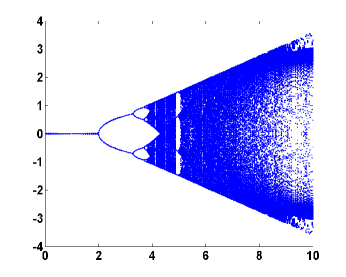
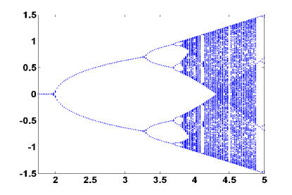
Figure 1: The chaotic map of the iteration formula (26) in the firefly algorithm and the transition between from periodic/multiple states to chaos.

In an even simpler 1-D case, we can set $y_{t}=g-\mbox{\boldmath$x$}_{i}^{t}$, and we have

$$y_{t+1}=y_{t}-\beta_{0}e^{-\gamma y_{t}^{2}}y_{t}.$$ (23)

Using the approximation of $0<\gamma y_{t}^{2}\ll 1$, we have

$$y_{t+1}=y_{t}-\beta_{0}(1-\gamma y_{t}^{2})y_{t}=y_{t}[1-\beta_{0}(1-\gamma y_{t}^{2})].$$ (24)

We can see that $\gamma$ is a scaling parameter which only affects the scales/size of the firefly movement. In fact, we can let $u_{t}=\sqrt{\gamma}y_{t}$ and rewrite the above the equation as

$$u_{t+1}=u_{t}[1-\beta_{0}(1-u_{t}^{2})],$$ (25)

or directly from (23)

$$u_{t+1}=u_{t}[1-\beta_{0}e^{-u_{t}^{2}}].$$ (26)

These equations can be analyzed easily using the same methodology for studying the well-known logistic map

$$u_{t}=\lambda u_{t}(1-u_{t}).$$ (27)

The chaotic map is shown in Fig. 1, and the focus on the transition from periodic multiple states to chaotic behaviour is shown in the same figure.

As we can see from Fig. 1 that convergence can be achieved for $\beta_{0}<2$. There is a transition from periodic to chaos at $\beta_{0}\approx 4$. This may be surprising, as the aim of designing a metaheuristic algorithm is to try to find the optimal solution efficiently and accurately. However, chaotic behaviour is not necessarily a nuisance, in fact, we can use it to the advantage of the firefly algorithm. Simple chaotic characteristics from (27) can often be used as an efficient mixing technique for generating diverse solutions. Statistically, the logistic mapping (27) for $\lambda=4$ for the initial states in (0,1) corresponds a beta distribution

$$B(u,p,q)=\frac{\Gamma(p+q)}{\Gamma(p)\Gamma(q)}u^{p-1}(1-u)^{q-1},$$ (28)

when $p=q=1/2$. Here $\Gamma(z)$ is the Gamma function

$$\Gamma(z)=\int_{0}^{\infty}t^{z-1}e^{-t}dt.$$ (29)

In the case when $z=n$ is an integer, we have $\Gamma(n)=(n-1)!$. In addition, $\Gamma(1/2)=\sqrt{\pi}$. From the algorithm implementation point of view, we can use higher attractiveness $\beta_{0}$ during the early stage of iterations so that the fireflies can explore, even chaotically, the search space more effectively. As the search continues and convergence approaches, we can reduce the attractiveness $\beta_{0}$ gradually, which may increase the overall efficiency of the algorithm. Obviously, more studies are highly needed to confirm this.

4 Essential Components of Metaheuristics

The efficiency of metaheuristic algorithms can be attributed to the fact that they imitate the best features in nature, especially the selection of the fittest in biological systems which have evolved by natural selection over millions of years.

Metaheuristics can be considered as an efficient way to produce acceptable solutions by trial and error to a complex problem in a reasonably practical time. The complexity of the problem of interest makes it impossible to search every possible solution or combination, the aim is to find good feasible solution in an acceptable timescale. There is no guarantee that the best solutions can be found, and we even do not know whether an algorithm will work and why if it does work. The idea is to have an efficient but practical algorithm that will work most the time and is able to produce good quality solutions. Among the found quality solutions, it is expected some of them are nearly optimal, though there is no guarantee for such optimality.

The main components of any metaheuristic algorithms are: intensification and diversification, or exploitation and exploration${}^{{\scriptsize~{}\cite[cite]{[\@@bibref{}{Blum,Yang2}{}{}]}}}$. Diversification means to generate diverse solutions so as to explore the search space on the global scale, while intensification means to focus on the search in a local region by exploiting the information that a current good solution is found in this region. This is in combination with with the selection of the best solutions.

The selection of the best ensures that the solutions will converge to the optimality. On the other hand, the diversification via randomization avoids the solutions being trapped at local optima, while increases the diversity of the solutions. The good combination of these two major components will usually ensure that the global optimality is achievable.

The fine balance between these two components is very important to the overall efficiency and performance of an algorithm. Too little exploration and too much exploitation could cause the system to be trapped in local optima, which makes it very difficult or even impossible to find the global optimum. On the other hand, if too much exploration but too little exploitation, it may be difficult for the system to converge and thus slows down the overall search performance. The proper balance itself is an optimization problem, and one of the main tasks of designing new algorithms is to find a certain balance concerning this optimality and/or tradeoff. Furthermore, just exploitation and exploration are not enough. During the search, we have to use a proper mechanism or criterion to select the best solutions. The most common criterion is to use the survival of the fittest, that is to keep updating the the current best found so far. In addition, certain elitism is often used, and this is to ensure the best or fittest solutions are not lost, and should be passed onto the next generations.

5 Randomization Techniques

As discussed earlier, an important component in swarm intelligence and modern metaheuristics is randomization, which enables an algorithm to have the ability to jump out of any local optimum so as to search globally. Randomization can also be used for local search around the current best if steps are limited to a local region. Fine-tuning the randomness and balance of local search and global search is crucially important in controlling the performance of any metaheuristic algorithm.

Randomization techniques can be a very simple method using uniform distributions, or more complex methods as those used in Monte Carlo simulations${}^{{\scriptsize~{}\cite[cite]{[\@@bibref{}{Sobol}{}{}]}}}$. They can also be more elaborate, from Brownian random walks to Lévy flights.

5.1 Random Walks

A random walk is a random process which consists of taking a series of consecutive random steps. Mathematically speaking, let $S_{N}$ denotes the sum of each consecutive random step $X_{i}$, then $S_{N}$ forms a random walk

$$S_{N}=\sum_{i=1}^{N}X_{i}=X_{1}+...+X_{N},$$ (30)

where $X_{i}$ is a random step drawn from a random distribution. This relationship can also be written as a recursive formula

$$S_{N}=\sum_{i=1}^{N-1}+X_{N}=S_{N-1}+X_{N},$$ (31)

which means the next state $S_{N}$ will only depend the current existing state $S_{N-1}$ and the motion or transition $X_{N}$ from the existing state to the next state. This is typically the main property of a Markov chain to be introduced later. Here the step size or length in a random walk can be fixed or varying. Random walks have many applications in physics, economics, statistics, computer sciences, environmental science and engineering.

In theory, as the number of steps $N$ increases, the central limit theorem implies that the random walk (31) should approaches a Gaussian distribution. In addition, there is no reason why each step length should be fixed. In fact, the step size can also vary according to a known distribution. If the step length obeys the Gaussian distribution, the random walk becomes the Brownian motion${}^{{\scriptsize~{}\cite[cite]{[\@@bibref{}{Gutow,Yang2}{}{}]}}}$.

As the mean of particle locations is obviously zero, their variance will increase linearly with $t$. In general, in the $d$-dimensional space, the variance of Brownian random walks can be written as

$$\sigma^{2}(t)=|v_{0}|^{2}t^{2}+(2dD)t,$$ (32)

where $v_{0}$ is the drift velocity of the system. Here $D=s^{2}/(2\tau)$ is the effective diffusion coefficient which is related to the step length $s$ over a short time interval $\tau$ during each jump.

Therefore, the Brownian motion $B(t)$ essentially obeys a Gaussian distribution with zero mean and time-dependent variance. That is, $B(t)\sim N(0,\sigma^{2}(t))$ where $\sim$ means the random variance obeys the distribution on the right-hand side; that is, samples should be drawn from the distribution. A diffusion process can be viewed as a series of Brownian motion, and the motion obeys the Gaussian distribution. For this reason, standard diffusion is often referred to as the Gaussian diffusion. If the motion at each step is not Gaussian, then the diffusion is called non-Gaussian diffusion. If the step length obeys other distribution, we have to deal with more generalized random walk. A very special case is when the step length obeys the Lévy distribution, such a random walk is called Lévy flight or Lévy walk.

5.2 Lévy Distribution and Lévy Flights

In nature, animals search for food in a random or quasi-random manner. In general, the foraging path of an animal is effectively a random walk because the next move is based on the current location/state and the transition probability to the next location. Which direction it chooses depends implicitly on a probability which can be modelled mathematically. For example, various studies have shown that the flight behaviour of many animals and insects has demonstrated the typical characteristics of Lévy flights${}^{{\scriptsize~{}\cite[cite]{[\@@bibref{}{Pav,Romos,Reynolds,Reynolds2}{}{}]}}}$. For example, a recent study by Reynolds and Frye shows that fruit flies or Drosophila melanogaster, explore their landscape using a series of straight flight paths punctuated by a sudden $90^{o}$ turn, leading to a Lévy-flight-style intermittent scale-free search pattern${}^{{\scriptsize~{}\cite[cite]{[\@@bibref{}{Reynolds}{}{}]}}}$. Subsequently, such behaviour has been applied to optimization and optimal search, and preliminary results show its promising capability ${}^{{\scriptsize~{}\cite[cite]{[\@@bibref{}{Viswan,Pav}{}{}]}}}$.

Broadly speaking, Lévy flights are a random walk whose step length is drawn from the Lévy distribution, often in terms of a simple power-law formula $L(s)\sim|s|^{-1-\beta}$ where $0<\beta\leq 2$ is an index. Mathematically speaking, a simple version of Lévy distribution can be defined as

$$L(s,\gamma,\mu)=\left\{\begin{array}[]{lllll}\sqrt{\frac{\gamma}{2\pi}}\exp[-\frac{\gamma}{2(s-\mu)}]\frac{1}{(s-\mu)^{3/2}},&0<\mu<s<\infty\\ \\ 0&\textrm{otherwise},\end{array}\right.$$ (33)

where $\mu>0$ is a minimum step and $\gamma$ is a scale parameter. Clearly, as $s\rightarrow\infty$, we have

$$L(s,\gamma,\mu)\approx\sqrt{\frac{\gamma}{2\pi}}\frac{1}{s^{3/2}}.$$ (34)

This is a special case of the generalized Lévy distribution${}^{{\scriptsize~{}\cite[cite]{[\@@bibref{}{Gutow,Nol}{}{}]}}}$.

In general, Lévy distribution should be defined in terms of Fourier transform

$$F(k)=\exp[-\alpha|k|^{\beta}],\quad 0<\beta\leq 2,$$ (35)

where $\alpha$ is a scale parameter. The inverse of this integral is not easy, as it does not have analytical form, except for a few special cases.

For the case of $\beta=2$, we have

$$F(k)=\exp[-\alpha k^{2}],$$ (36)

whose inverse Fourier transform corresponds to a Gaussian distribution. Another special case is $\beta=1$, and we have

$$F(k)=\exp[-\alpha|k|],$$ (37)

which corresponds to a Cauchy distribution

$$p(x,\gamma,\mu)=\frac{1}{\pi}\frac{\gamma}{\gamma^{2}+(x-\mu)^{2}},$$ (38)

where $\mu$ is the location parameter, while $\gamma$ controls the scale of this distribution.

For the general case, the inverse integral

$$L(s)=\frac{1}{\pi}\int_{0}^{\infty}\cos(ks)\exp[-\alpha|k|^{\beta}]dk,$$ (39)

can be estimated only when $s$ is large. We have

$$L(s)\rightarrow\frac{\alpha\;\beta\;\Gamma(\beta)\sin(\pi\beta/2)}{\pi|s|^{1+\beta}},\quad s\rightarrow\infty.$$ (40)

Lévy flights are more efficient than Brownian random walks in exploring unknown, large-scale search space. There are many reasons to explain this efficiency, and one of them is due to the fact that the variance of Lévy flights

$$\sigma^{2}(t)\sim t^{3-\beta},\quad 1\leq\beta\leq 2,$$ (41)

increases much faster than the linear relationship (i.e., $\sigma^{2}(t)\sim t$) of Brownian random walks.

From the implementation point of view, the generation of random numbers with Lévy flights consists of two steps: the choice of a random direction and the generation of steps which obey the chosen Lévy distribution. The generation of a direction should be drawn from a uniform distribution, while the generation of steps is quite tricky. There are a few ways of achieving this, but one of the most efficient and yet straightforward ways is to use the so-called Mantegna algorithm for a symmetric Lévy stable distribution${}^{{\scriptsize~{}\cite[cite]{[\@@bibref{}{Mant,Nol}{}{}]}}}$. Here ‘symmetric’ means that the steps can be positive and negative.

A random variable $U$ and its probability distribution can be called stable if a linear combination of its two identical copies (or $U_{1}$ and $U_{2}$) obeys the same distribution. That is, $aU_{1}+bU_{2}$ has the same distribution as $cU+d$ where $a,b>0$ and $c,d\in\Re$. If $d=0$, it is called strictly stable. Gaussian, Cauchy and Lévy distributions are all stable distributions.

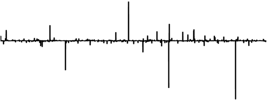
Figure 2: Steps drawn from a Lévy distribution ($\beta=1$) using Mantegna’s algorithm.

In Mantegna’s algorithm${}^{{\scriptsize~{}\cite[cite]{[\@@bibref{}{Mant}{}{}]}}}$, the step length $s$ can be calculated by

$$s=\frac{u}{|v|^{1/\beta}},$$ (42)

where $u$ and $v$ are drawn from normal distributions. That is

$$u\sim N(0,\sigma_{u}^{2}),\quad v\sim N(0,\sigma_{v}^{2}),$$ (43)

where

$$\sigma_{u}=\Big{\{}\frac{\Gamma(1+\beta)\sin(\pi\beta/2)}{\Gamma[(1+\beta)/2]\;\beta\;2^{(\beta-1)/2}}\Big{\}}^{1/\beta},\quad\sigma_{v}=1.$$ (44)

This distribution (for $s$) obeys the expected Lévy distribution for $|s|\geq|s_{0}|$ where $s_{0}$ is the smallest step. In principle, $|s_{0}|\gg 0$, but in reality $s_{0}$ can be taken as a sensible value such as $s_{0}=0.1$ to $1$.

Fig. 2 shows the 250 steps drawn from a Lévy distribution with $\beta=1$, while Fig. 3 shows the path of Lévy flights of 250 steps starting from $(0,0)$. It is worth pointing out that a power-law distribution is often linked to some scale-free characteristics, and Lévy flights can thus show self-similarity and fractal behavior in the flight patterns.

Studies show that Lévy flights can maximize the efficiency of resource searches in uncertain environments. In fact, Lévy flights have been observed among foraging patterns of albatrosses and fruit flies, and spider monkeys${}^{{\scriptsize~{}\cite[cite]{[\@@bibref{}{Pav,Romos,Reynolds,Reynolds2,Viswan}{}{}]}}}$. In addition, Lévy flights have many applications. Many physical phenomena such as the diffusion of fluorenscent molecules, cooling behavior and noise could show Lévy-flight characteristics under the right conditions${}^{{\scriptsize~{}\cite[cite]{[\@@bibref{}{Reynolds2}{}{}]}}}$.

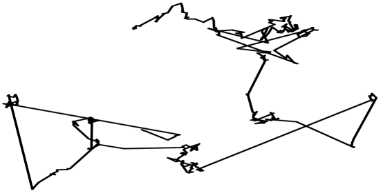
Figure 3: Schematic representation of 2D Lévy flights.

5.3 Step Size in Random Walks

As random walks are widely used for randomization and local search, a proper step size is very important. In the generic equation

$$\mbox{\boldmath$x$}^{t+1}=\mbox{\boldmath$x$}^{t}+s\;\mbox{\boldmath$\epsilon$}_{t},$$ (45)

$\mbox{\boldmath$\epsilon$}_{t}$ is drawn from a standard normal distribution with zero mean and unity standard deviation. Here the step size $s$ determines how far a random walker (e.g., an agent or particle in metaheuristics) can go for a fixed number of iterations.

If $s$ is too large, then the new solution $\mbox{\boldmath$x$}^{t+1}$ generated will be too far away from the old solution (or more often the current best). Then, such a move is unlikely to be accepted. If $s$ is too small, the change is too small to be significant, and consequently such search is not efficient. So a proper step size is important to maintain the search as efficient as possible.

From the theory of simple isotropic random walks, we know that the average distance $r$ traveled in the $d$-dimension space is

$$r^{2}=2dDt,$$ (46)

where $D=s^{2}/2\tau$ is the effective diffusion coefficient. Here $s$ is the step size or distance traveled at each jump, and $\tau$ is the time taken for each jump. The above equation implies that

$$s^{2}=\frac{\tau\;r^{2}}{t\;d}.$$ (47)

For a typical length scale $L$ of a dimension of interest, the local search is typically limited in a region of $L/10$. That is, $r=L/10$. As the iterations are discrete, we can take $\tau=1$. Typically in metaheuristics, we can expect that the number of generations is usually $t=100$ to $1000$, which means that

$$s\approx\frac{r}{\sqrt{td}}=\frac{L/10}{\sqrt{t\;d}}.$$ (48)

For $d=1$ and $t=100$, we have $s=0.01L$, while $s=0.001L$ for $d=10$ and $t=1000$. As step sizes could differ from variable to variable, a step size ratio $s/L$ is more generic. Therefore, we can use $s/L=0.001$ to $0.01$ for most problems.

5.4 Swarm Intelligence and Markov Chains

From the discussion and analysis of metaheuristic algorithms, we know that there is no mathematical framework in general to provide insights into the working mechanisms, the stability and convergence of a give algorithm. Despite the increasing popularity of metaheuristic, mathematical analysis remains fragmental, and many open problems need urgent attention.

From the statistical point of view, most metaheuristic algorithms can be viewed in the framework of Markov chains${}^{{\scriptsize~{}\cite[cite]{[\@@bibref{}{Fishman,Sobol}{}{}]}}}$. For example, simulated annealing${}^{{\scriptsize~{}\cite[cite]{[\@@bibref{}{Kirk}{}{}]}}}$ is a Markov chain, as the next state or new solution in SA only depends on the current state/solution and the transition probability. For a given Markov chain with certain ergodicity, a stability probability distribution and convergence can be achieved. In fact, it has been proved that SA will always converge if the system is cooled down slowly enough and the annealling process runs long enough.

Now if look at the PSO closely using the framework of Markov chain Monte Carlo${}^{{\scriptsize~{}\cite[cite]{[\@@bibref{}{Gamer,Geyer,Ghate}{}{}]}}}$, each particle in PSO essentially forms a Markov chain, though this Markov chain is biased towards to the current best, as the transition probability often leads to the acceptance of the move towards the current global best. In addition, the multiple Markov chains are interacting in terms of partly deterministic attraction movement. Therefore, the mathematical analysis concerning of the rate of convergence of PSO is very difficult, if not impossible. Similarly, other swarm-based metaheuristics such as firefly algorithms and cuckoo search can also be viewed as interacting Markov chains. There is no doubt that any theoretical advance in understanding multiple interacting Markov chains will gain tremendous insight in understanding how the swarm intelligence behaves and may consequently lead to the design of better or new metaheuristics.

6 Discussions

Swarm-based metaheuristics are becoming increasingly popular, though theoretical framework and analysis still lack behind. Many important problems still remain unsolved. Firstly, there is no general convergence analysis for all metaheuristics, apart from some fragmental and yet important work concerning PSO and SA. Secondly, the choice of algorithm-dependent parameters such as population size and probability is currently based on experience and parametric studies. Thirdly, stopping criteria are also a bit arbitrary, though fixed accuracy or maximum number of iterations are widely used.

In addition, there is no agreed measure to compare the performance of any two algorithms. People either compare the number of function evaluations for a given objective value or compare the objective values for a given number of functional evaluations. These results are often affected by algorithm-dependent parameters or way of actual implementation. As randomness is an integrated part of metaheuristics, statistical measures should be used. A general, statistical framework for performance comparison and algorithm evaluations is highly needed.

Furthermore, no-free-lunch theorems${}^{{\scriptsize~{}\cite[cite]{[\@@bibref{}{Wolpert}{}{}]}}}$ may have some important implications in metaheuristics, however, the basic assumptions of these theorems may be questionable. Besides, these theorems are valid for single objective optimization, and they remain open questions for multiobjective.

Finally, the current understanding of swarm intelligence is still very limited. How multiagents interact with simple rules can lead to complex behaviour, self-organization and eventually intelligence still remains a major mystery. Any insight with theoretical basis may have important implications to many areas, not only metaheuristics and optimization, but also neural networks and machine learning. Whatever the future developments will be, there is no doubt that swarm-based algorithms and swarm intelligence will play an ever more important role in science and engineering.

References

- [1] A. Ayesh, Swarm-based emotion modelling, Int. J. Bio-Inspired Computation, 118-124 (2009).
- [2] W. J. Bell, Searching Behaviour: The Behavioural Ecology of Finding Resources, Chapman & Hall, London, (1991).
- [3] C. Blum and A. Roli, Metaheuristics in combinatorial optimization: Overview and conceptural comparison, ACM Comput. Surv., 35, 268-308 (2003).
- [4] A. Chatterjee and P. Siarry, Nonlinear inertia variation for dynamic adapation in particle swarm optimization, Comp. Oper. Research, 33, 859-871 (2006).
- [5] S. Chowdhury, G. S. Dulikravich, R. J. Moral, Modified predator-prey algoirthm for constrained and unconstrained multi-objective optimization, Int. J. Mathematical Modelling and Numerical Optimisation, 1, 1-38 (2009).
- [6] M. Clerc, J. Kennedy, The particle swarm - explosion, stability, and convergence in a multidimensional complex space, IEEE Trans. Evolutionary Computation, 6, 58-73 (2002).
- [7] Cui, Z. H., and Zeng, J. C., A modified particle swarm optimization predicted by velocity, GECCO 2005, pp. 277–278 (2005).
- [8] Cui, Z. H., and Cai, X. J., Integral particle swarm optimization with dispersed accelerator information, Fundam. Inform., 95, 427–447 (2009).
- [9] Dorigo, M., Optimization, Learning and Natural Algorithms, PhD thesis, Politecnico di Milano, Italy, (1992).
- [10] A. P. Engelbrecht, Fundamentals of Computational Swarm Intelligence, Wiley, (2005).
- [11] G. S. Fishman, Monte Carlo: Concepts, Algorithms and Applications, Springer, New York, (1995).
- [12] D. Gamerman, Markov Chain Monte Carlo, Chapman & Hall/CRC, (1997).
- [13] Z. W. Geem and W. E. Roper, Various continuous harmony search algorithms for web-based hydrologic parameter estimation, Int. J. Mathematical Modelling and Numerical Optimisation, 1, 213-226 (2010).
- [14] C. J. Geyer, Practical Markov Chain Monte Carlo, Statistical Science, 7, 473-511 (1992).
- [15] A. Ghate and R. Smith, Adaptive search with stochastic acceptance probabilities for global optimization, Operations Research Lett., 36, 285-290 (2008).
- [16] R. Gross and M. Dorigo, Towards group transport by swarms of robots, Int. J. Bio-Inspired Computation, 1, 1-13 (2009).
- [17] M. Gutowski, Lévy flights as an underlying mechanism for global optimization algorithms, ArXiv Mathematical Physics e-Prints, June, (2001).
- [18] J. Kennedy and R. C. Eberhart, Particle swarm optimization, in: Proc. of IEEE International Conference on Neural Networks, Piscataway, NJ. pp. 1942-1948 (1995).
- [19] J. Holland, Adaptation in Natural and Artificial systems, University of Michigan Press, Ann Anbor, (1975).
- [20] J. Kennedy, R. C. Eberhart, Swarm intelligence, Academic Press, 2001.
- [21] S. Kirkpatrick, C. D. Gellat and M. P. Vecchi, Optimization by simulated annealing, Science, 220, 670-680 (1983).
- [22] R. N. Mantegna, Fast, accurate algorithm for numerical simulation of Levy stable stochastic processes, Physical Review E, 49, 4677-4683 (1994).
- [23] J. P. Nolan, Stable distributions: models for heavy-tailed data, American University, (2009).
- [24] I. Pavlyukevich, Lévy flights, non-local search and simulated annealing, J. Computational Physics, 226, 1830-1844 (2007).
- [25] G. Ramos-Fernandez, J. L. Mateos, O. Miramontes, G. Cocho, H. Larralde, B. Ayala-Orozco, Lévy walk patterns in the foraging movements of spider monkeys (Ateles geoffroyi), Behav. Ecol. Sociobiol., 55, 223-230 (2004).
- [26] A. M. Reynolds and M. A. Frye, Free-flight odor tracking in Drosophila is consistent with an optimal intermittent scale-free search, PLoS One, 2, e354 (2007).
- [27] A. M. Reynolds and C. J. Rhodes, The Lévy fligth paradigm: random search patterns and mechanisms, Ecology, 90, 877-887 (2009).
- [28] I. M. Sobol, A Primer for the Monte Carlo Method, CRC Press, (1994).
- [29] E. G. Talbi, Metaheuristics: From Design to Implementation, Wiley, (2009).
- [30] G. M. Viswanathan, S. V. Buldyrev, S. Havlin, M. G. E. da Luz, E. P. Raposo, and H. E. Stanley, Lévy flight search patterns of wandering albatrosses, Nature, 381, 413-415 (1996).
- [31] D. H. Wolpert and W. G. Macready, No free lunch theorems for optimisation, IEEE Transaction on Evolutionary Computation, 1, 67-82 (1997).
- [32] X. S. Yang, Nature-Inspired Metaheuristic Algorithms, Luniver Press, (2008).
- [33] X. S. Yang, X. Engineering Optimization: An Introduction with Metaheuristic Applications, John Wiley & Sons.
- [34] X. S. Yang, Firefly algorithm, stochastic test functions and design optimisation, Int. J. Bio-Inspired Computation, 2, 78–84 (2010).
- [35] X. S. Yang and S. Deb, Engineering optimization by cuckoo search, Int. J. Math. Modelling & Num. Optimization, 1, 330-343 (2010).
- [36] X. S. Yang, A new metaheuristic bat-inspired algorithm, in: Nature Inspired Cooperative Strategies for Optimization (NICSO 2010) (Eds. J. R. Gonzalez et al.), Springer, SCI 284, 65-74 (2010b).