Higgs Boson Studies at the Tevatron

Abstract

We combine searches by the CDF and D0 Collaborations for the standard model Higgs boson with mass in the range 90–200 GeV$/c^{2}$ produced in the gluon-gluon fusion, $WH$, $ZH$, $t{\bar{t}}H$, and vector boson fusion processes, and decaying in the $H\rightarrow b{\bar{b}}$, $H\rightarrow W^{+}W^{-}$, $H\rightarrow ZZ$, $H\rightarrow\tau^{+}\tau^{-}$, and $H\rightarrow\gamma\gamma$ modes. The data correspond to integrated luminosities of up to 10 fb^-1 and were collected at the Fermilab Tevatron in $p{\bar{p}}$ collisions at $\sqrt{s}=1.96$ TeV. The searches are also interpreted in the context of fermiophobic and fourth generation models. We observe a significant excess of events in the mass range between 115 and 140 GeV/$c^{2}$. The local significance corresponds to 3.0 standard deviations at $m_{H}=125$ GeV/$c^{2}$, consistent with the mass of the Higgs boson observed at the LHC, and we expect a local significance of 1.9 standard deviations. We separately combine searches for $H\to b\bar{b}$, $H\to W^{+}W^{-}$, $H\rightarrow\tau^{+}\tau^{-}$, and $H\rightarrow\gamma\gamma$. The observed signal strengths in all channels are consistent with the presence of a standard model Higgs boson with a mass of 125 GeV/$c^{2}$.

I Introduction

Within the standard model (SM) gws , spontaneous breaking of electroweak symmetry gives mass to the $W$ and $Z$ bosons hig , and to the fundamental fermions via their Yukawa interactions with the Higgs field. In the SM, the symmetry-breaking mechanism predicts the existence of one neutral scalar particle, the Higgs boson, whose mass ($m_{H}$) is a free parameter.

Precision electroweak data, including the recently updated measurements of the $W$-boson and top-quark masses from the CDF and D0 Collaborations top ; w , yield an indirect constraint on the allowed mass of the Higgs boson, $m_{H}<152$ GeV/$c^{2}$ lepewwg , at the 95% confidence level (C.L.) clnote . Direct searches at LEP2 exclude SM Higgs boson masses below 114.4 GeV/$c^{2}$ sm- . The ATLAS and CMS Collaborations at the Large Hadron Collider (LHC) have recently reported the observation of a new boson with mass of around 125 GeV/$c^{2}$ atlas ; cms . Much of the sensitivity of the LHC searches comes from gluon-gluon fusion ($gg\rightarrow H$) production and Higgs boson decays to $\gamma\gamma$, $ZZ$, and $W^{+}W^{-}$. Published searches for associated production $VH\rightarrow Vb{\bar{b}}$ at the LHC, where $V=W$ or $Z$ atl (a); cms (a), have not yet reached sensitivity to SM Higgs boson production. The CDF and D0 Collaborations have recently reported combined evidence for a particle, with a mass consistent with that of the new boson observed at LHC, produced in association with a $W$ or $Z$ boson and decaying to a bottom-antibottom quark pair tevhbbprl .

In this article, we combine the most recent results of SM Higgs boson searches in $p\bar{p}$ collisions at $\sqrt{s}=1.96$ TeV  using the full Tevatron Run II integrated luminosity of up to 10 fb^-1 per experiment. The analyses combined here seek signals of Higgs bosons in the mass range 90–200 GeV/$c^{2}$, produced in association with a vector boson ($q\bar{q}\rightarrow VH$), in association with top quarks, through gluon-gluon fusion, and through vector boson fusion (VBF) ($q\bar{q}\rightarrow q^{\prime}\bar{q}^{\prime}H$). The Higgs boson decay modes studied are $H\rightarrow b{\bar{b}}$, $H\rightarrow W^{+}W^{-}$, $H\rightarrow ZZ$, $H\rightarrow\tau^{+}\tau^{-}$, and $H\rightarrow\gamma\gamma$. For Higgs boson masses greater than 130 GeV$/c^{2}$, searches for $H\rightarrow W^{+}W^{-}$ decays with subsequent leptonic $W$ decays provide the greatest sensitivity. Below 130 GeV$/c^{2}$, sensitivity comes mainly from associated $VH$ production, with the $H$ boson decaying to $b\bar{b}$ and the $W$ or $Z$ boson decaying leptonically. While we present our results in the full mass range, we also focus specifically on the mass hypothesis $m_{H}=125$ GeV/$c^{2}$, due to the recent LHC findings. Specifically, we show the sensitivity of the searches over the full mass range to a SM Higgs boson signal with $m_{H}=125$ GeV/$c^{2}$. Previous Tevatron SM combinations, focused respectively on the $H\rightarrow b{\bar{b}}$ and $H\rightarrow W^{+}W^{-}$ decay modes, are published in Refs. tevhbbprl ; tev (b). The results presented here are based on the combinations of the searches from each experiment as published in Refs. cdfprd ; d0prd .

This article is structured as follows. Section II discusses the simulation methods used to predict the yields from the signal and SM background processes. Section III briefly describes the CDF and D0 detectors. Section IV describes the event selections used by the various analyses and Section V presents the data. Section VI provides a brief introduction to the statistical procedures used and Section VII discusses the different sources of systematic uncertainties and how they are controlled. Sections VIII and IX present the results in the contexts of the SM and extensions to it. Section X summarizes the article.

II Event simulation

Higgs boson signal events are simulated using the leading-order (LO) calculation from pythia pyt , with CTEQ5L (CDF) and CTEQ6L1 (D0) cte parton distribution functions (PDFs). The normalization of these Monte Carlo (MC) samples is obtained using the highest-order cross-section calculation available for the corresponding production process. The cross section for the gluon-gluon fusion process is calculated at next-to-next-to-leading order (NNLO) in quantum chromodynamics (QCD) with soft gluon resummation to next-to-next-to-leading-log (NNLL) accuracy anastasiou ; grazzinideflorian . These calculations include two-loop electroweak corrections, and also three-loop ${\cal{O}}(\alpha\alpha_{s})$ corrections. The WH and ZH cross-section calculations are performed at NNLO precision in QCD and next-to-leading-order (NLO) precision in the electroweak corrections vht . The VBF cross section is computed at NNLO in QCD vbfnnlo , and the electroweak corrections are computed with the hawk program hawk . The $t{\bar{t}}H$ production cross sections are taken from Ref. tth . The signal production cross sections are computed using the MSTW2008 PDF set mstw08 , except for the $t{\bar{t}}H$ production cross section which uses the CTEQ6M cte PDF set. The Higgs boson decay branching fractions are from Ref. lhc (a) and rely on calculations using hdecay hde and prophecy4f pro . The distribution of the transverse momentum ($p_{T}$) of the Higgs boson in the pythia-generated gluon-fusion sample is reweighted to match the $p_{T}$ as calculated by hqt Higgs_pT , at NNLL and NNLO accuracy.

We model SM and instrumental background processes using a mixture of MC and data-driven methods. In the CDF analyses, backgrounds from SM processes with electroweak gauge bosons or top quarks are modeled using pythia, alpgen Man , mc@nlo MC@ , and herwig her . For D0, these backgrounds are modeled using pythia, alpgen, and singletop com . An interface to pythia provides parton showering and hadronization for generators without this functionality.

Diboson (WW, WZ, ZZ) MC samples are normalized using the NLO calculations from mcfm mcf . For top-quark-pair production ($t{\bar{t}}$), we use a production cross section of $7.04\pm 0.49$ pb moc , which is based on a top-quark mass of 173 GeV/$c^{2}$ top and MSTW 2008 PDFs mstw08 . The single-top-quark production cross section is taken to be $3.15\pm 0.31$ pb kid . For many analyses, the V+jet processes are normalized using the NNLO cross section calculations of Ref. v-xs , though in some cases data-driven techniques are used. Likewise, the normalization of the instrumental, multijet and, for the CDF searches, the V+heavy-flavor jet backgrounds hfj are constrained from data samples where the expected signal-to-background ratio is several orders of magnitude smaller than in the search samples. For the D0 searches, the V+light-flavor is normalized to data in a control region, and the V+heavy-flavor normalization, relative to the V+light-flavor, is taken from mcfm. In addition, for the D0 searches, prior to $b$-tagging btag V+jets samples are compared to data and corrections applied to mitigate any discrepancies in kinematic distributions.

All MC samples are processed through a geant geant simulation of the detector, and reconstructed in the same way as data. The effects of instrumental noise and additional $p{\bar{p}}$ interactions are modeled using MC in the CDF analyses, while recorded data from randomly selected beam crossings with the same instantaneous luminosity profile as data are overlaid on to the MC events in the D0 analyses. In the entire Run II data sample, the average number of reconstructed primary vertices is approximately 3 – including the hard scatter.

For the $H\rightarrow W^{+}W^{-}$ analyses, the dominant irreducible background process is diboson production, while the dominant reducible backgrounds are $Z/\gamma^{*}+$jets, $t\bar{t}$, $W$+$\gamma$, $W$+jets, and multijet production where in the latter three cases photons or jets can be misidentified as leptons. For the analyses targeting $H\rightarrow b\bar{b}$ the main backgrounds originate from $V$+heavy-flavor-jets and $t\bar{t}$ production.

III Detectors and object reconstruction

The CDF and D0 detectors have central trackers surrounded by hermetic calorimeters and muon detectors and are designed to study the products of 1.96 TeV proton-antiproton collisions cdf (e); d0d . Most searches combined here use the complete Tevatron data sample, which corresponds to up to 10 fb^-1 depending on the experiment and the search channel, after data-quality requirements. The online event selections (triggers) rely on fast reconstruction of combinations of high-$p_{T}$ lepton candidates, jets, and missing transverse energy ($\not\!\!E_{T}$), defined below. To maximize sensitivity, all events satisfying any trigger requirement from the complete suite of triggers used for data taking are considered whenever possible. For instance, while most of the $H\rightarrow W^{+}W^{-}$ candidate events are selected by single-lepton and dilepton triggers, a gain in efficiency of up to 20%, depending on the channel, is achieved by including events that pass lepton+jets and lepton$+\mbox{$E\kern-6.00006pt/_{T}$}$ triggers.

High-quality electron candidates are identified by associating charged-particle tracks with deposits of energy in the electromagnetic calorimeters when both measurements are available. High-quality muon candidates are identified by associating tracks with hits in the muon detectors surrounding the calorimeters in the CDF and D0 detectors. Lepton candidates are categorized based on the quality of the contributing measurements. Tight selection requirements yield samples of leptons with low background rates from hadrons or jets of hadrons misidentified as leptons. Looser requirements are designed to increase the acceptance for lepton candidates with poorly measured or partially missing information, with resulting higher rates for backgrounds. To optimize the sensitivity of the combined results, events that are selected with high-quality leptons are analyzed separately from those with low-quality leptons.

Jets are clustered from energy deposits in the electromagnetic and hadronic calorimeters and, in some analyses, combine information from charged particle tracks to improve purity or energy resolution. The transverse energy vector ${\vec{E}_{T}}$ of a calorimeter energy deposit is $E\sin\theta{\hat{n}}$, where $E$ is the measured energy, $\theta$ is the angle with respect to the proton beam axis of a line drawn from the collision point to the energy deposit, and ${\hat{n}}$ is a unit vector in the plane perpendicular to the beam pointing along that line. The missing transverse energy $\not\!\!E_{T}$ is the magnitude of the vector opposite to the sum of the ${\vec{E}_{T}}$ vectors measured in the calorimeter, after propagation of all corrections to the calorimetric objects and for identified muons (which deposit only small amounts of energy in the calorimeters) contributing to the signal topology. Further details of the object reconstruction algorithms used in the Higgs boson searches can be found in the references for the individual analyses (see Tables 1 and 2).

IV Event selection

Event selections are similar in the CDF and D0 analyses, typically consisting of a preselection based on event topology and kinematics. Multivariate analysis (MVA) techniques mva are used to combine several discriminating variables into a single final discriminant that is used in the statistical interpretation to compute upper limits, $p$-values, and fitted cross sections. Each channel is divided into exclusive sub-channels according to various lepton, jet multiplicity, and $b$-tagging characterization criteria. This procedure groups events with similar signal-to-background ratio to optimize the overall sensitivity. Such subdivision allows, for example, the efficient use of poorly reconstructed leptons or those in the forward region, the exploitation of the different dominant signal and backgrounds when training the MVAs separately in each sub-channel, or reduction of the impact of systematic uncertainties. The MVAs are trained separately at each value of $m_{H}$ in their respective mass ranges, in 5 GeV/$c^{2}$ steps.

For the analyses exploiting the $H\rightarrow b\bar{b}$ decay, $b$-tagging and dijet mass resolution are of great importance. Both collaborations have developed multivariate approaches to maximize the performance of the $b$-tagging algorithms. The CDF $b$-tagging algorithm is based on an MVA tag , and depending on the chosen operating point provides $b$-tagging efficiencies of 50%–70% with misidentification rates for light ($u$, $d$, $s$, and gluon) jets of 0.5%–6%. In the D0 analyses, the MVA builds and improves upon the previous neural network $b$-tagger Aba ; dzZHv2 and achieves identification efficiencies of about 80% (50%) for $b$ jets for a light jet misidentification rate of about 10% (0.5%).

The decay width of the SM Higgs boson is predicted to be much smaller than the experimental dijet mass resolution, which is typically 15% of the mean reconstructed mass. A SM Higgs boson signal would appear as a broad enhancement in the reconstructed di-$b$-jet mass distribution. The CDF and D0 Collaborations search for $H\rightarrow b{\bar{b}}$ produced in association with a leptonically decaying $W$ boson, or a leptonically or invisibly decaying $Z$ boson. CDF also contributes searches for $WH+ZH\rightarrow jjb{\bar{b}}$ and $t{\bar{t}}H\rightarrow t{\bar{t}}b{\bar{b}}$, where in the latter case one of the top quarks decays to a leptonically decaying $W$ boson.

Both collaborations search for the $H\rightarrow W^{+}W^{-}$ signal in which both $W$ bosons decay leptonically by selecting events with large missing transverse energy and two oppositely-charged, isolated leptons. The presence of neutrinos in the final state prevents reconstruction of the Higgs boson mass. Other observables are used for separating the signal from background. For example, the azimuthal angle between the leptons in signal events is smaller on average than that in background events due to the scalar nature of the Higgs boson and parity violation in $W^{\pm}$ decays. Furthermore, the missing transverse momentum is larger and the total transverse energy of the jets is lower than they are typically in background events. The D0 Collaboration also includes channels in which one of the $W$ bosons in the $H\rightarrow W^{+}W^{-}$ process decays leptonically and the other hadronically.

Although the primary sensitivity at low mass ($m_{H}\leq 130$ GeV/$c^{2}$) is provided by the $H\rightarrow b\bar{b}$ analyses and at high mass ($m_{H}>130$ GeV/$c^{2}$) by the $H\rightarrow W^{+}W^{-}$ analyses, significant additional sensitivity is achieved by the inclusion of other channels. Both collaborations contribute analyses searching for Higgs bosons decaying into tri-lepton final states, tau-lepton pairs and diphoton pairs. The full list of channels included is shown in Tables 1 and 2 which summarize, for the CDF and D0 analyses respectively, the integrated luminosities, the Higgs boson mass ranges over which the searches are performed, and references to further details for each analysis.

Table 1: Luminosities, explored mass ranges, and references for the different processes and final states ($\ell$ = $e$ or $\mu$, and $\tau_{\rm{had}}$ denotes a hadronic tau-lepton decay) for the CDF analyses. The generic labels “$1\times$”, “$2\times$”, “$3\times$”, and “$4\times$” refer to separations based on lepton or photon categories. The analyses are grouped in five categories, corresponding to the Higgs boson decay mode to which the analysis is most sensitive: $H\to b\bar{b}$, $H\to W^{+}W^{-}$, $H\to\tau^{+}\tau^{-}$, $H\to\gamma\gamma$, and $H\to ZZ$.

Channel		Luminosity	$m_{H}$ range	Reference
		(fb-1)	(GeV/$c^{2}$)
$WH\rightarrow\ell\nu b\bar{b}$ 2-jet channels    4$\times$(5 $b$-tag categories)		9.45	90–150	cdfWH
$WH\rightarrow\ell\nu b\bar{b}$ 3-jet channels    3$\times$(2 $b$-tag categories)		9.45	90–150	cdfWH
$ZH\rightarrow\nu\bar{\nu}b\bar{b}$    (3 $b$-tag categories)		9.45	90–150	cdfmetbb
$ZH\rightarrow\ell^{+}\ell^{-}b\bar{b}$ 2-jet channels    2$\times$(4 $b$-tag categories)	$H\rightarrow b\bar{b}$	9.45	90–150	cdfZH
$ZH\rightarrow\ell^{+}\ell^{-}b\bar{b}$ 3-jet channels    2$\times$(4 $b$-tag categories)		9.45	90–150	cdfZH
$WH+ZH\rightarrow jjb{\bar{b}}$     (2 $b$-tag categories)		9.45	100–150	cdfjjbb
$t\bar{t}H\rightarrow W^{+}bW^{-}\bar{b}b\bar{b}$     (4 jets,5 jets,$\geq$6 jets)$\times$(5 $b$-tag categories)		9.45	100-150	cdfttHLep
$H\rightarrow W^{+}W^{-}$    2$\times$(0 jets)+2$\times$(1 jet)+1$\times$($\geq$2 jets)+1$\times$(low-$m_{\ell\ell}$)		9.7	110–200	cdfHWW
$H\rightarrow W^{+}W^{-}$    ($e$-$\tau_{\rm{had}}$)+($\mu$-$\tau_{\rm{had}}$)		9.7	130–200	cdfHWW
$WH\rightarrow WW^{+}W^{-}$    (same-sign leptons)+(tri-leptons)	$H\rightarrow W^{+}W^{-}$	9.7	110–200	cdfHWW
$WH\rightarrow WW^{+}W^{-}$    (tri-leptons with 1 $\tau_{\rm{had}}$)		9.7	130–200	cdfHWW
$ZH\rightarrow ZW^{+}W^{-}$    (tri-leptons with 1 jet,$\geq$2 jets)		9.7	110–200	cdfHWW
$H\rightarrow\tau^{+}\tau^{-}$    (1 jet)+($\geq$2 jets)	$H\rightarrow\tau^{+}\tau^{-}$	6.0	100–150	cdfHtt
$H\rightarrow\gamma\gamma$     1$\times$(0 jet)+1$\times$($\geq$1 jet)+3$\times$(all jets)	$H\rightarrow\gamma\gamma$	10.0	100–150	cdfHgg
$H\rightarrow ZZ$    (four leptons)	$H\rightarrow ZZ$	9.7	120–200	cdfHZZ

Table 2: Luminosities, explored mass ranges, and references for the different processes and final states ($\ell=e$ or $\mu$, and $\tau_{\rm{had}}$ denotes a hadronic tau-lepton decay) for the D0 analyses. The generic labels “$1\times$”, “$2\times$”, “$3\times$”, and “$4\times$” refer to separations based on lepton, photon or background characterization categories. The analyses are grouped in four categories, corresponding to the Higgs boson decay mode to which the analysis is most sensitive: $H\to b\bar{b}$, $H\to W^{+}W^{-}$, $H\to\tau^{+}\tau^{-}$, and $H\to\gamma\gamma$.

Channel		Luminosity	$m_{H}$ range	Reference
		(fb-1)	(GeV/$c^{2}$)
$WH\rightarrow\ell\nu b\bar{b}$ 2-jet channels    2$\times$(4 $b$-tag categories)		9.7	90–150	dzWHl-jul12 ; dzWHl
$WH\rightarrow\ell\nu b\bar{b}$ 3-jet channels    2$\times$(4 $b$-tag categories)		9.7	90–150	dzWHl-jul12 ; dzWHl
$ZH\rightarrow\nu\bar{\nu}b\bar{b}$    (2 $b$-tag categories)	$H\to b\bar{b}$	9.5	100–150	dzZHv2
$ZH\rightarrow\ell^{+}\ell^{-}b\bar{b}$    2$\times$(2 $b$-tag)$\times$(4 lepton categories)		9.7	90–150	dzZHll1-jul12 ; dzZHll1
$H\rightarrow W^{+}W^{-}\rightarrow\ell^{\pm}\nu\ell^{\mp}\nu$    2$\times$(0 jets,1 jet,$\geq$2 jets)		9.7	115–200	dzHWW
$H~{}+~{}X\rightarrow W^{+}W^{-}\rightarrow\mu^{\mp}\nu\tau_{\rm{had}}^{\pm}\nu$    (3 $\tau$ categories)		7.3	115–200	dzVHt1
$H\rightarrow W^{+}W^{-}\rightarrow\ell\bar{\nu}jj$    2$\times$(2 $b$-tag categories)$\times$(2 jets, 3 jets)	$H\to W^{+}W^{-}$	9.7	100–200	dzWHl
$VH\rightarrow e^{\pm}\mu^{\pm}+X$		9.7	100–200	dzWWW2
$VH\rightarrow\ell\ell\ell+X$ ($\mu\mu e$, 3 $\times$ $e\mu\mu$)		9.7	100–200	dzWWW2
$VH\rightarrow\ell\bar{\nu}jjjj$    2$\times$($\geq$4 jets)		9.7	100-200	dzWHl
$VH\rightarrow\tau_{\rm{had}}\tau_{\rm{had}}\mu+X$    (3 $\tau$ categories)	$H\rightarrow\tau^{+}\tau^{-}$	8.6	100-150	dzWWW2
$H$+$X$$\rightarrow$$\ell^{\pm}\tau^{\mp}_{\rm{had}}jj$    2$\times$(3 $\tau$ categories)		9.7	105–150	dzVHt2
$H\rightarrow\gamma\gamma$    (4 categories)	$H\rightarrow\gamma\gamma$	9.6	100-150	dzHgg

V Candidate distribution

The number of contributing channels is large, and several different kinds of discriminating varibles are used. Visual comparison of the observed data with the predictions is challenging in some of the sub-channels due to low data counts. For a more robust comparison, we display the data from all the sub-channels together, aggregating bins with similar signal to background ratios ($s/b$) from all contributing sub-channels. We collect the signal predictions, the background predictions, and the data in narrow bins of $s/b$, summing the contributions from bins in the final discriminant histograms in the sub-channels. A fit of the background model (see Section VI) to the data is performed before this aggregation procedure, in order to provide the best prediction for the background model in bins with the highest sensitivity. The classification of analysis events according to their $s/b$ preserves the importance of each of the events in the histogram, to the extent that they are not added to other events that are selected with different $s/b$. This representation of the data is not used to compute the final results, since the distribution indiscriminately sums unrelated backgrounds which are fit separately. It does, however, provide a guide to how much individual events contribute to the results and how well the signal is separated from backgrounds in the combined search. The resulting distribution of $\log_{10}(s/b)$ is shown for $m_{H}=125$ GeV/$c^{2}$ in Fig. 1, demonstrating agreement with background over five orders of magnitude.

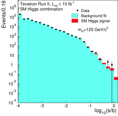
Figure 1: (color online). Distribution of $\log_{10}(s/b)$, for the data from all contributing Higgs boson search channels from CDF and D0, for $m_{H}=125$ GeV/$c^{2}$. The data are shown with points, and the expected signal is shown stacked on top of the backgrounds, which are fit to the data within their systematic uncertainties. The error bars shown on the data correspond in each bin to the square root of the observed data count. Underflows and overflows are collected into the leftmost and rightmost bins, respectively.

VI STATISTICAL TECHNIQUES

The results are interpreted using both Bayesian and modified frequentist techniques, separately at each value of $m_{H}$, as was done previously tev (b); tevhbbprl ; pdg . The two methods yield results that are numerically consistent; limits on the Higgs boson production rate typically agree within 5% at each value of $m_{H}$, and with a 1% deviation when averaged over all positive and negative departures. For simplicity, when summarizing the results, we quote one set of values as the default, and the a priori decision made for the earlier Tevatron combinations to use the Bayesian method is retained here. Both methods use the distributions of the final discriminants, and not only the total event counts passing selection requirements.

Each of the techniques is built on a combined likelihood (including prior probability densities on systematic uncertainties, $\pi({\vec{\theta}})$) based on the product of likelihoods for the individual channels, each of which is a product over histogram bins,

$${\cal{L}}(R,{\vec{s}},{\vec{b}}|{\vec{n}},{\vec{\theta}})\!\times\!\pi({\vec{\theta}})=\prod_{i=1}^{N_{\rm C}}\prod_{j=1}^{N_{\rm bins}}\mu_{ij}^{n_{ij}}\frac{e^{-\mu_{ij}}}{n_{ij}!}\times\prod_{k=1}^{n_{\rm sys}}e^{-\theta_{k}^{2}/2},$$ (1)

where the first product is over the number of channels ($N_{\rm C}$) and the second product is over histogram bins containing $n_{ij}$ events, binned in ranges of the final discriminants used for the individual analyses. The predictions for the bin contents are $\mu_{ij}=R\times s_{ij}({\vec{\theta}})+b_{ij}({\vec{\theta}})$ for channel $i$ and histogram bin $j$, where $s_{ij}$ and $b_{ij}$ represent the expected SM signal and background in the bin, and $R$ is a scaling factor applied to the signal. By scaling all signal contributions by the same factor we assume that the relative contributions of the different processes at each $m_{H}$ are as predicted by the SM. Systematic uncertainties are parametrized by the dependence of $s_{ij}$ and $b_{ij}$ on ${\vec{\theta}}$. Each of the $n_{\rm sys}$ components of ${\vec{\theta}}$, $\theta_{k}$, corresponds to a single independent source of systematic uncertainty scaled by its standard deviation, and each parameter may affect the predictions of several sources of signal and background in different channels, thus accounting for correlations. Gaussian prior densities are assumed for the nuisance parameters, truncated to ensure that no prediction is negative.

In the Bayesian calculation, we assume a uniform prior probability density for non-negative values of $R$ and integrate the likelihood function multiplied by prior densities for the nuisance parameters to obtain the posterior density for $R$. The observed 95% credibility level upper limit on $R$, $R_{95}^{\rm{obs}}$, is the value of $R$ such that the integral of the posterior density of $R$ from zero to $R_{95}^{\rm{obs}}$ corresponds to 95% of the integral of $R$ from zero to infinity. The expected distribution of $R_{95}$ is computed in an ensemble of simulated experimental outcomes assuming no signal is present. In each simulated outcome, random values of the nuisance parameters are drawn from their prior densities. A combined measurement of the cross section for Higgs boson production times the branching fraction ${\cal B}(H\rightarrow XX)$, in units of the SM production rate, is given by $R^{\rm{fit}}$, which is the value of $R$ that maximizes the posterior density. The 68% credibility interval, which corresponds to one standard deviation (s.d.), is quoted as the smallest interval containing 68% of the integral of the posterior.

We also perform calculations with the modified frequentist technique ${\rm CL}_{\rm s}$ pdg , using a log-likelihood ratio (LLR) as the test statistic: LLR$=-2\ln\frac{p({\mathrm{data}}|s+b)}{p({\mathrm{data}}|b)}$, where $p({\mathrm{data}}|s+b)$ and $p({\mathrm{data}}|b)$ are the probabilities that the data (either simulated or experimental data) are drawn from distributions predicted under the signal-plus-background and background-only hypotheses, respectively. The probabilities $p$ are computed using the best-fit values of the parameters $\theta_{k}$, separately for each of the two hypotheses pflh . The use of these fits extends the procedure used at LEP lep , improving the sensitivity when the expected signals are small and the uncertainties on the backgrounds are large. The ${\rm CL}_{\rm s}$ technique involves computing two $p$-values, ${\rm CL}_{\rm b}=p$(LLR $\geq$ LLR${}_{\mathrm{obs}}|b$), where LLR_obs is the value of the test statistic computed for the data, and ${\rm CL}_{\rm s+b}=p$(LLR$\geq$ LLR${}_{\mathrm{obs}}|s+b$). To compute limits, we use the ratio of $p$-values, ${\rm CL}_{\rm s}={\rm CL}_{\rm s+b}/{\rm CL}_{\rm b}$. If ${\rm CL}_{\rm s}<0.05$ for a particular choice of the signal-plus-background hypothesis, parametrized by the signal scale factor $R$, that hypothesis is excluded at least at the 95% C.L. The value of $R_{95}^{\rm{obs}}$ in the CL_s method is the smallest value of $R$ excluded at the 95% C.L. The expected limit is computed using the median LLR value expected in the background-only hypothesis. Systematic uncertainties are included by fluctuating around their Gaussian priors the predictions for $s_{ij}$ and $b_{ij}$ when generating the pseudoexperiments used to compute CL_s+b and CL_b.

In this framework, a second estimate of the signal rate, $R^{\rm{fit}}_{\rm{profile}}$ is computed, maximizing the likelihood as a function of the unconstrained signal rate $R$ and the nuisance parameters $\theta_{k}$. This estimate of the combined signal rate may differ from the Bayesian calculation of $R^{\rm{fit}}$ when the likelihood function deviates from a Gaussian form, since the best fit depends on the likelihood near the maximum and the Bayesian calculation integrates over all values of the nuisance parameters which result in positive signal and background rates in all histogram bins.

VII Systematic Uncertainties

Systematic uncertainties are evaluated for each final state, background, and signal process. Uncertainties that modify only the normalization and uncertainties that change the shape of the final discriminant distribution are included. To study the shape uncertainties on the distributions of the final discriminants, the relevant parameter is varied within one standard deviation of its uncertainty and the full analysis repeated using the modified distribution. For example, for the jet energy scale and resolution, the parameters of the energy scale and resolution are varied within one s.d. of their uncertainties and the analysis carried out using the kinematic distributions of the modified jets, also including the changes in sample composition resulting from the change in the jet energy parameters. No retraining of the MVAs is performed during the propagation of systematic uncertainties to the distributions of the discriminants. Correlations between signal and background, across different channels within an experiment and across the two experiments are taken into account. Full details on the treatment of the systematic uncertainties in the individual channels can be found in the relevant references.

The uncertainties on the inclusive signal production cross sections are estimated from the variations in the factorization and renormalization scale, which include the impact of uncalculated higher-order corrections, uncertainties due to PDFs, and the dependence on the strong coupling constant, $\alpha_{s}$, as recommended by the PDF4LHC working group pdf_uncertainties ; ggH01jetUncert . The resulting uncertainties on the inclusive VH and VBF production rates are taken to be 7% and 5%, respectively vht . Uncertainties on the branching fractions are taken from Ref. HBR-err .

For analyses focusing on $gg\rightarrow H$ production that divide events into categories based on the number of reconstructed jets, the uncertainties associated with the renormalization and factorization scale are estimated following Ref. errMatr . By propagating the uncorrelated uncertainties of the NNLL inclusive anastasiou ; grazzinideflorian , NLO $\geq 1$ jet  ggH01jetUncert , and NLO $\geq 2$ jets campbellh2j cross sections to the exclusive ${gg\to H}+0$ jet, $\geq 1$ jet, and $\geq 2$ jets rates, an uncertainty matrix containing correlated and uncorrelated uncertainty contributions between exclusive jet categories is obtained. The total uncertainty on $gg\rightarrow H$ production originating from these contributions varies from 10% to 35% in individual channels depending on the number of jets in the final state. The PDF uncertainties are evaluated following Refs. anastasiou ; ggH01jetUncert .

Significant sources of uncertainty for all analyses are the integrated luminosities used to normalize the expected signal yield and MC-based backgrounds, and the cross sections for the simulated backgrounds. For the former, uncertainties of 6% (CDF) and 6.1% (D0) are used, with 4% arising from the inelastic $p{\bar{p}}$ cross section which is taken to be 100% correlated between CDF and D0. Cross-section uncertainties of 6% and 7% are used for diboson and $t\bar{t}$ production respectively. The uncertainty on the expected multijet background in each channel is dominated by the statistics of the data sample from which it is estimated and varies from 10% to 30%.

Sources of systematic uncertainty that affect both the normalization and the shape of the final discriminant distribution include jet energy scale (1–4)%, jet energy resolution (1–3)%, lepton identification, trigger efficiencies, and $b$-tagging. Uncertainties on lepton identification and trigger efficiencies range from 2% to 6% and are applied to both the signal and MC-based background predictions. These uncertainties are estimated from data-based methods separately by CDF and D0, and differ based on lepton flavor and identification category. The $b$-tag efficiencies and mistag rates are similarly constrained by auxiliary data samples, such as inclusive jet data or $t{\bar{t}}$ events. The uncertainty on the per-jet $b$-tag efficiency is approximately 4%, and the mistag uncertainties vary between 7% and 15%.

For the analyses targeting the $H\rightarrow b\bar{b}$ decay, the largest sources of uncertainty on the dominant backgrounds are the rates of $V+$heavy flavor jets, which are typically 20–30% of the predicted values. Using constraints from the data, the uncertainties on these rates are typically 8% or less. The data samples in the $V+$jets selections prior to $b$-tagging are used as control samples to constrain systematic uncertainties in the MC modeling of the energies and angles of jets. Any residual discrepancy coming from the difference between light- and heavy-flavor components is shown to be smaller than the systematic uncertainties associated with the generator or the correction procedures themselves.

A total of 326 independent sources of systematic uncertainty are included in the combination of the Higgs boson search results at $m_{H}=125$ GeV/$c^{2}$, not including the independent uncertainties in each bin of each template from limited Monte Carlo (or data) statistics. The uncertainties that are considered correlated between CDF and D0 are those on the differential and inclusive theoretical production cross section predictions for the Higgs boson signals (itemized by PDF$+\alpha_{s}$ and scales), the Higgs boson decay branching fractions, the $t{\bar{t}}$, single top, and diboson background processes, and the correlated part of the luminosity estimate. All other uncertainties are associated with parameters whose central values are estimated using techniques specific to the experiments and the analysis channels. We consider these uncorrelated so as not to extrapolate fit information improperly from one channel or experiment to another where the central value or the uncertainty scale may be different.

VIII Results - Standard model interpretation

VIII.1 Diboson Production

To validate our background modeling and methodology, independent measurements of SM diboson production in the same final states used for the SM Higgs searches are carried out. The high mass analyses measure $p\bar{p}\rightarrow VV^{\prime}$ cross sections, while the low mass analyses target $VZ(\to b\bar{b})$ production. The data sample, reconstruction, process modeling, uncertainties, and sub-channel divisions are identical to those of the SM Higgs boson searches. However, discriminant functions are trained to distinguish the contributions of SM diboson production from those of other backgrounds, and potential contributions from Higgs boson production are not considered. By way of illustration, below, we focus on VZ production.

The NLO SM cross section for VZ production times the branching fraction of $Z\rightarrow b\bar{b}$ is 0.68 $\pm$ 0.05 pb mcf ; pdg . This is about six times larger than the 0.12 $\pm$ 0.01 pb vht ; lhc (a) cross section times branching fraction of $H(\to b\bar{b})V$ for a 125 GeV/$c^{2}$ SM Higgs boson, but the associated background is larger, due to the distribution of the dijet invariant mass in the $V$+jets events. WW production is considered as background. The measured cross section, using the MVA discriminants, for VZ is $3.0\pm 0.6$ (stat) $\pm 0.7$ (syst) pb whereas the SM prediction is $4.4\pm 0.3$ pb mcf . The combined background-subtracted dijet-mass distribution for the VZ analysis is shown in Fig. 2 for illustration.

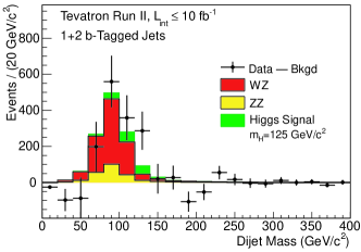
Figure 2: (color online). Background-subtracted distribution of the reconstructed dijet mass, summed over CDF and D0’s channels contributing to the VZ analysis. The VZ signal and the background contributions are fit to the data, and the fitted background is subtracted. The fitted VZ and expected SM Higgs ($m_{H}=125$ GeV/$c^{2}$) contributions are shown with filled histograms. The error bars shown on the data points correspond in each bin to the square root of the sum of the expected signal and background yields.

The VZ signal and the background contributions are fit to the data, and the fitted background is then subtracted. Also shown is the contribution expected from a SM Higgs boson with $m_{H}=125$ GeV/$c^{2}$. The VV^′ boson cross sections measured by the high mass analyses are likewise in good agreement with SM predictions cdfww ; d0prd .

VIII.2 Higgs boson combination using all decay modes

For the search for the Higgs boson, the results produced by the multivariate analyses can be visualized by combining the histograms of the final discriminants, adding the contents of bins with similar signal-to-background ratio ($s/b$) as shown in Fig. 1. Figure 3 shows the signal expectation and the data with the background subtracted, as a function of the $s/b$ of the collected bins, for the combined search for a Higgs boson with mass $m_{H}=125$ GeV/$c^{2}$. The background model is fit to the data, allowing the nuisance parameters to vary within their constraints. The uncertainties on the background predictions in each bin are those after the fit. An excess of events in the highest $s/b$ bins relative to the background-only expectation is observed.

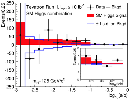
Figure 3: (color online). Background-subtracted distribution of the discriminant histograms, summed for bins with similar signal-to-background ratio ($s/b$) over all contributing Higgs boson search channels from CDF and D0, for $m_{H}=125$ GeV/$c^{2}$. The background is fit to the data, and the uncertainty on the background, shown with the unfilled histogram, is after the fit. The signal model, scaled to the SM expectation, is shown with a filled histogram. The error bars shown on the data points correspond in each bin to the square root of the sum of the expected signal and background yields.

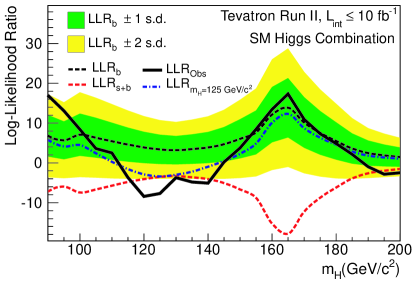
Figure 4: (color online). The log-likelihood ratio LLR as a function of Higgs boson mass for all of CDF and D0’s SM Higgs boson searches in all decay modes combined. The solid line shows the observed LLR values, the dark long-dashed line shows the median expectation assuming no Higgs boson signal is present, and the dark- and light-shaded bands correspond, respectively, to the regions encompassing one and two s.d. fluctuations around the background-only expectation. The red long-dashed line shows the median expectation assuming a SM Higgs boson signal is present at each value of $m_{H}$ in turn. The blue short-dashed line shows the median expected LLR assuming the SM Higgs boson is present at $m_{H}=125$ GeV/$c^{2}$.

Figure 4 displays the LLR distributions for the combined analyses as functions of $m_{H}$. Included are the median of the LLR distributions for the background-only hypothesis (LLR_b), the signal-plus-background hypothesis (LLR_s+b), and the observed value for the data (LLR_obs). For mass hypotheses of 95 GeV/$c^{2}$ and less, fewer channels are available for combination, giving rise to the behavior of the limits shown. The shaded bands represent the one and two s.d. departures for LLR_b centered on the median. These results are listed in Table 3. The separation between the medians of the LLR_b and LLR_s+b distributions provides a measure of the discriminating power of the search. The widths of the one- and two-s.d. LLR_b bands indicate the width of the LLR_b distribution, assuming no signal and that fluctuations originate from statistical fluctuations and systematic effects only. The value of LLR_obs relative to LLR_s+b and LLR_b indicates whether the data distribution more closely resembles the distributions expected if a signal is present (i.e., the LLR_s+b distribution, which is negative by construction) or only background is present. The significance of departures of LLR_obs from LLR_b can be evaluated by the width of the LLR_b bands. The separation of the median signal-plus-background and background-only hypotheses is about two s.d., or greater, for Higgs boson masses up to $\approx$ 185 GeV/$c^{2}$. The data are consistent with the background-only hypothesis (the black dashed line) at masses smaller than $\approx$ 110 GeV/$c^{2}$ and above approximately 145 GeV/$c^{2}$. A slight excess is seen above approximately 195 GeV/$c^{2}$, where our ability to separate the two hypotheses is limited. For $m_{H}$ from 115 to 140 GeV/$c^{2}$, an excess above two s.d. in the data with respect to the SM background expectation has an amplitude consistent with the expectation for a standard model Higgs boson (dashed red line). Additionally, the LLR curve under the hypothesis that a SM Higgs boson is present with $m_{H}=125$ GeV/$c^{2}$ is shown. This signal-injected-LLR curve has a similar shape to the observed one. While the search for a 125 GeV/$c^{2}$ Higgs boson is optimized to find a Higgs boson of that mass, the excess of events over the SM background estimates also affects the results of Higgs boson searches at other masses. Nearby masses are the most affected, but the expected presence of $H\to W^{+}W^{-}$ decays for a 125 GeV/$c^{2}$ Higgs boson implies a small expected excess in the $H\to W^{+}W^{-}$ searches at all masses due to the poor reconstructed mass resolution in this final state.

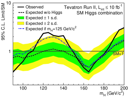
Figure 5: (color online). Observed and median expected (for the background-only hypothesis) 95% C.L. Bayesian upper production limits expressed as multiples of the SM cross section as a function of Higgs boson mass for the combined CDF and D0 searches in all decay modes. The dark- and light-shaded bands indicate, respectively, the one and two s.d probability regions in which the limits are expected to fluctuate in the absence of signal. The blue short-dashed line shows median expected limits assuming the SM Higgs boson is present at $m_{H}=125$ GeV/$c^{2}$.

Table 3: Log-likelihood ratio (LLR) values obtained from the combination of all of CDF and D0’s Higgs boson search channels using the ${\rm CL}_{\rm s}$ method.

$m_{H}$ (GeV/$c^{2}$)	LLRobs	LLRs+b	LLR${}_{b}^{-2\sigma}$	LLR${}_{b}^{-1\sigma}$	LLRb	LLR${}_{b}^{+1\sigma}$	LLR${}_{b}^{+2\sigma}$
90	17.02	$-7.24$	17.31	12.08	6.84	1.61	$-3.62$
95	13.07	$-5.96$	15.21	10.44	5.68	0.91	$-3.85$
100	8.39	$-7.44$	17.73	12.40	7.08	1.76	$-3.56$
105	3.62	$-6.69$	16.38	11.35	6.32	1.29	$-3.74$
110	2.53	$-5.73$	14.79	10.12	5.45	0.78	$-3.89$
115	$-3.67$	$-4.81$	13.17	8.88	4.59	0.31	$-3.98$
120	$-8.44$	$-4.09$	11.76	7.82	3.88	$-0.06$	$-4.00$
125	$-7.72$	$-3.52$	10.76	7.07	3.39	$-0.29$	$-3.97$
130	$-3.74$	$-3.30$	10.31	6.74	3.18	$-0.39$	$-3.95$
135	$-4.81$	$-3.64$	10.89	7.17	3.45	$-0.26$	$-3.98$
140	$-5.08$	$-4.09$	11.72	7.79	3.86	$-0.07$	$-4.00$
145	0.20	$-5.07$	13.35	9.02	4.69	0.36	$-3.97$
150	3.72	$-6.68$	15.87	10.95	6.04	1.12	$-3.79$
155	8.44	$-8.80$	18.72	13.18	7.65	2.12	$-3.41$
160	13.45	$-15.25$	26.04	19.08	12.12	5.15	$-1.81$
165	17.33	$-17.81$	28.76	21.31	13.87	6.42	$-1.03$
170	10.93	$-12.26$	22.87	16.50	10.13	3.77	$-2.60$
175	7.33	$-8.77$	18.50	13.02	7.53	2.04	$-3.45$
180	4.86	$-6.17$	14.87	10.18	5.50	0.81	$-3.88$
185	2.14	$-3.92$	11.23	7.42	3.62	$-0.19$	$-3.99$
190	$-0.99$	$-2.61$	8.73	5.60	2.46	$-0.68$	$-3.81$
195	$-2.83$	$-1.98$	7.34	4.60	1.87	$-0.87$	$-3.60$
200	$-2.50$	$-1.53$	6.29	3.88	1.46	$-0.96$	$-3.37$

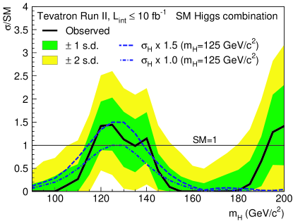
Figure 6: (color online). The best-fit signal cross section expressed as a ratio to the SM cross section as a function of Higgs boson mass for all of CDF and D0’s SM Higgs boson searches in all decay modes combined. The dark- and light-shaded bands show the one and two s.d. uncertainty ranges on the fitted signal, respectively. Also shown with blue lines are the median fitted cross sections expected for a SM Higgs boson with $m_{H}=125$ GeV/$c^{2}$ at signal strengths of 1.0 times (short-dashed) and 1.5 times (long-dashed) the SM prediction.

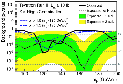
Figure 7: (color online). The solid black line shows the background $p$-value as a function of $m_{H}$ for all of CDF and D0’s SM Higgs boson searches in all decay modes combined. The dotted black line shows the median expected values assuming a SM signal is present, evaluated separately at each $m_{H}$. The associated dark- and light-shaded bands indicate the one and two s.d. fluctuations of possible experimental outcomes under this scenario. The blue lines show the median expected $p$-values assuming the SM Higgs boson is present with $m_{H}$=125 GeV/$c^{2}$ at signal strengths of 1.0 times (short-dashed) and 1.5 times (long-dashed) the SM prediction.

The upper limit on SM Higgs boson production as a function of $m_{H}$ is extracted in the range 90–200 GeV/$c^{2}$ in terms of $R_{95}^{\mathrm{obs}}$, the ratio of the observed limit to the predicted SM rate. The ratios of the 95% C.L. expected and observed limit to the SM cross section using the Bayesian method are shown in Fig. 5 for the combined CDF and D0 analyses. The observed and median-expected ratios are listed for the tested Higgs boson masses in Table 4, as obtained by the Bayesian and the ${\rm CL}_{\rm s}$ methods.

Table 4: Ratios of observed and median expected (for the background-only hypothesis) 95% C.L. upper production limits to the SM cross section as a function of the Higgs boson mass for the combined CDF and D0 searches in all decay modes, obtained using the Bayesian and ${\rm CL}_{\rm s}$ methods.

	Bayesian		${\rm CL}_{\rm s}$
$m_{H}$ (GeV/$c^{2}$)	$R_{95}^{\mathrm{obs}}$	$R_{95}^{\mathrm{exp}}$	$R_{95}^{\mathrm{obs}}$	$R_{95}^{\mathrm{exp}}$
90	0.37	0.74	0.39	0.74
95	0.48	0.80	0.49	0.81
100	0.62	0.72	0.62	0.73
105	0.89	0.77	0.93	0.77
110	1.02	0.82	1.03	0.83
115	1.63	0.90	1.67	0.91
120	2.33	1.00	2.40	0.99
125	2.44	1.06	2.62	1.07
130	2.13	1.11	2.10	1.10
135	2.03	1.04	2.12	1.06
140	2.10	1.01	2.08	1.00
145	1.35	0.88	1.29	0.90
150	0.94	0.79	0.91	0.78
155	0.64	0.69	0.62	0.68
160	0.46	0.51	0.45	0.51
165	0.37	0.47	0.36	0.47
170	0.54	0.57	0.53	0.57
175	0.71	0.68	0.68	0.68
180	0.87	0.81	0.86	0.82
185	1.20	1.02	1.18	1.04
190	1.86	1.29	1.86	1.27
195	2.74	1.44	2.64	1.48
200	3.07	1.66	2.97	1.67

Intersections of piecewise linear interpolations of the observed and expected rate limits with the SM=1 line are used to quote ranges of Higgs boson masses that are excluded and that are expected to be excluded. The regions of Higgs boson masses excluded at the 95% C.L. are 90 $<m_{H}<$ 109 GeV/$c^{2}$ and 149 $<m_{H}<$ 182 GeV/$c^{2}$. The expected exclusion regions are 90 $<m_{H}<$ 120 GeV/$c^{2}$ and 140 $<m_{H}<$ 184 GeV/$c^{2}$.

The observed excess for $m_{H}$ from 115 to 140 GeV/$c^{2}$ is driven by an excess of data events with respect to the background predictions in the most sensitive bins of the discriminant distributions, favoring the hypothesis that a signal is present. To characterize the compatibility of this excess with the signal-plus-background hypothesis, the best-fit rate cross section, $R^{\rm{fit}}$, is computed using the Bayesian calculation, and shown in Fig. 6. The measured signal strength is within 1 s.d. of the expectation for a SM Higgs boson in the range $115<m_{H}<140$ GeV$/c^{2}$, with maximal strength between 120 GeV$/c^{2}$ and 125 GeV$/c^{2}$. At 125 GeV$/c^{2}$, $R^{\rm{fit}}=1.44^{+0.49}_{-0.47}~{}({\rm{stat}})^{+0.33}_{-0.31}~{}({\rm{syst}})\pm 0.10~{}({\rm{theory}})$.

The significance of the excess in the data over the background prediction is computed at each hypothesized Higgs boson mass by calculating the local $p$-value under the background-only hypothesis using $R^{\rm{fit}}_{\rm{profile}}$, chosen a priori, as the test statistic. This $p$-value expresses the probability to obtain the value of $R^{\rm{fit}}_{\rm{profile}}$ observed in the data or larger, assuming a signal is absent. These $p$-values are shown in Fig. 7 along with the expected $p$-values assuming a SM signal is present, separately for each value of $m_{H}$. The median expected $p$-values assuming the SM Higgs boson is present with $m_{H}$=125 GeV/$c^{2}$ for signal strengths of 1.0 and 1.5 times the SM prediction are also shown. The median expected excess at $m_{H}=125$ GeV/$c^{2}$ corresponds to 1.9 standard deviations assuming the SM Higgs boson is present at that mass. The observed local significance at $m_{H}=125$ GeV/$c^{2}$ corresponds to 3.0 standard deviations. The maximum observed local significance is at $m_{H}=120$ GeV/$c^{2}$ and corresponds to 3.1 standard deviations. The fluctuations seen in the observed $p$-value as a function of the tested $m_{H}$ result from excesses seen in different search channels, as well as from point-to-point fluctuations due to the separate discriminants at each $m_{H}$, and are discussed in more detail below. The width of the dip in the observed $p$-values from 115 to 140 GeV/$c^{2}$ is consistent with the resolution of the combination of the $H\to b\bar{b}$ and $H\to W^{+}W^{-}$ channels, as illustrated by the injected signal curves in Fig. 7. The effective resolution of this search comes from two independent sources of information. The reconstructed candidate masses help constrain $m_{H}$, but more importantly, the expected cross sections times the relevant branching ratios for the $H\to b\bar{b}$ and $H\to W^{+}W^{-}$ channels are strong functions of $m_{H}$ in the SM. The observed excess in the $H\to b\bar{b}$ channels coupled with the slight excess in the $H\to W^{+}W^{-}$ channels determine the shape of the observed $p$-value as a function of $m_{H}$.

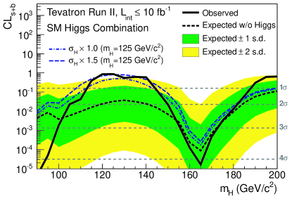
Figure 8: (color online). The solid black line shows the signal-plus-background $p$-value as a function of $m_{H}$ for all of CDF and D0’s SM Higgs boson searches in all decay modes combined. The dotted black line shows the median expected values assuming no SM signal is present, evaluated separately at each $m_{H}$. The associated dark and light-shaded bands indicate the one and two s.d. fluctuations of possible experimental outcomes under this scenario. The blue lines show the median expected $p$-values assuming the SM Higgs boson is present with $m_{H}$=125 GeV/$c^{2}$ at signal strengths of 1.0 times (short-dashed) and 1.5 times (long-dashed) the SM prediction.

Figure 8 shows the quantity ${\rm CL}_{\rm s+b}$, corresponding to the $p$-value for the signal-plus-background hypothesis. The observed value, along with the expected $p$-values assuming a signal is absent, are shown separately for each value of $m_{H}$. The median expected $p$-values assuming the SM Higgs boson is present with $m_{H}$=125 GeV/$c^{2}$ for signal strengths of 1.0 and 1.5 times the SM prediction are also shown. In the mass region from 115 to 140 GeV/$c^{2}$ the observed values above 50% indicate a high level of consistency with the signal-plus-background hypothesis.

We also separate CDF and D0’s searches into combinations focusing on the $H\to b\bar{b}$, $H\to W^{+}W^{-}$, $\ H\to\gamma\gamma$, and $\ H\to\tau^{+}\tau^{-}$ decay modes, and these are discussed in the following sections.

VIII.3 $H\rightarrow b{\bar{b}}$ Decay Mode

Below 130 GeV/$c^{2}$, the $H\rightarrow b{\bar{b}}$ searches contribute the majority of the search sensitivity. The $WH\rightarrow\ell\nu b\bar{b}$, $ZH\rightarrow\nu\bar{\nu}b\bar{b}$, and $ZH\rightarrow\ell^{+}\ell^{-}b\bar{b}$ channels from both experiments are included in this sub-combination. Two of the six contributing channels were updated for this sub-combination compared with that reported in Ref. tevhbbprl . The CDF $ZH\rightarrow\nu\bar{\nu}b\bar{b}$ cdfmetbb-jul12 analysis was updated to use a more powerful MVA b-tagging algorithm tag along with changes to the kinematic selections. The assignment of correlated systematic uncertainties between channels was updated in the D0 $WH\rightarrow\ell\nu b\bar{b}$ analysis dzWHl-jul12 . The observed LLR distribution is shown in Fig. 9, along with its expected values under the background-only and signal-plus-background hypotheses. The hypotheses that a SM Higgs boson is present with $m_{H}=125$ GeV/$c^{2}$ for signal strengths of 1.0 and 1.5 times the SM prediction are also given. The LLR values as a function of Higgs boson mass are listed in Table 5.

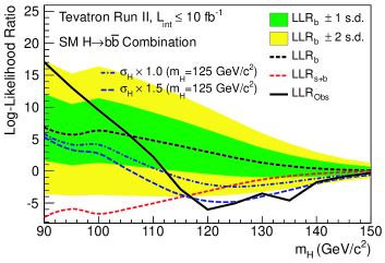
Figure 9: (color online). The log-likelihood ratio LLR as a function of Higgs boson mass from the combination of CDF and D0’s SM Higgs boson searches focusing on the $H\rightarrow b{\bar{b}}$ decay mode. The solid line shows the observed LLR values, the dark short-dashed line shows the median expectation assuming no Higgs boson signal is present, and the dark- and light-shaded bands correspond, respectively, to the regions encompassing one and two s.d. fluctuations around the background-only expectation. The red long-dashed line shows the median expectation assuming a SM Higgs boson signal is present at each value of $m_{H}$ in turn. The blue lines show the median expected LLR assuming the SM Higgs boson is present at $m_{H}=125$ GeV/$c^{2}$ with signal strengths of 1.0 times (short-dashed) and 1.5 times (long-dashed) the SM prediction.

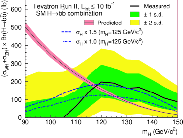
Figure 10: (color online). The best-fit signal cross section times branching ratio $(\sigma_{WH}+\sigma_{ZH})\times\mathcal{B}(H\rightarrow b{\bar{b}})$ as a function of Higgs boson mass from the combination of CDF and D0’s SM Higgs boson searches focusing on the $H\rightarrow b{\bar{b}}$ decay mode. The dark- and light-shaded bands show the one and two s.d. uncertainty ranges on the fitted signal, respectively. Also shown with blue lines are the median fitted cross sections expected for a SM Higgs boson with $m_{H}=125$ GeV/$c^{2}$ at signal strengths of 1.0 times (short-dashed) and 1.5 times (long-dashed) the SM prediction. The SM prediction is shown as the smooth, falling curve where the narrow band indicates the theoretical uncertainty.

Table 5: Log-likelihood ratio (LLR) values obtained from the combination of CDF and D0’s Higgs boson search channels focusing on the $H\rightarrow b{\bar{b}}$ decay mode using the ${\rm CL}_{\rm s}$ method.

$m_{H}$ (GeV/$c^{2}$)	LLRobs	LLRs+b	LLR${}_{b}^{-2\sigma}$	LLR${}_{b}^{-1\sigma}$	LLRb	LLR${}_{b}^{+1\sigma}$	LLR${}_{b}^{+2\sigma}$
90	17.02	$-7.24$	17.31	12.08	6.84	1.61	$-3.62$
95	13.07	$-5.96$	15.21	10.44	5.68	0.91	$-3.85$
100	9.50	$-6.71$	16.41	11.38	6.34	1.30	$-3.73$
105	6.09	$-6.00$	15.12	10.38	5.63	0.88	$-3.86$
110	2.21	$-5.06$	13.52	9.15	4.78	0.41	$-3.97$
115	$-2.84$	$-4.12$	11.83	7.87	3.91	$-0.04$	$-4.00$
120	$-6.05$	$-3.16$	9.91	6.45	2.99	$-0.47$	$-3.93$
125	$-5.05$	$-2.16$	7.88	4.99	2.09	$-0.80$	$-3.69$
130	$-3.53$	$-1.34$	5.89	3.60	1.31	$-0.98$	$-3.27$
135	$-4.60$	$-0.80$	4.28	2.52	0.77	$-0.98$	$-2.74$
140	$-1.77$	$-0.41$	2.93	1.67	0.40	$-0.87$	$-2.13$
145	$-0.86$	$-0.20$	1.95	1.07	0.19	$-0.68$	$-1.56$
150	$-0.31$	$-0.08$	1.23	0.66	0.08	$-0.49$	$-1.07$

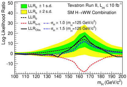
Figure 11: (color online). The log-likelihood ratio LLR as a function of Higgs boson mass from the combination of CDF and D0’s SM Higgs boson searches focusing on the $H\rightarrow W^{+}W^{-}$ decay mode. The solid line shows the observed LLR values, the dark short-dashed line shows the median expectation assuming no Higgs boson signal is present, and the dark- and light-shaded bands correspond, respectively, to the regions encompassing one and two s.d. fluctuations around the background-only expectation. The red long-dashed line shows the median expectation assuming a SM Higgs boson signal is present at each value of $m_{H}$ in turn. The blue lines show the median expected LLR assuming the SM Higgs boson is present at $m_{H}=125$ GeV/$c^{2}$ with signal strengths of 1.0 times (short-dashed) and 1.5 times (long-dashed) the SM prediction.

We multiply the best-fit rate cross section, $R^{\rm{fit}}$, for this sub-combination by the SM prediction for the associated-production cross section times the decay branching ratio ($\sigma_{WH}+\sigma_{ZH})\times\mathcal{B}(H\rightarrow b{\bar{b}})$, to obtain the observed value for this quantity. We show the fitted ($\sigma_{WH}+\sigma_{ZH})\times\mathcal{B}(H\rightarrow b{\bar{b}})$ as a function of $m_{H}$, along with the SM prediction, in Fig. 10. The figure also shows the expected cross section fits for each $m_{H}$, assuming that the SM Higgs boson with $m_{H}=125$ GeV/$c^{2}$ is present, both at the rate predicted by the SM, and also at a multiple of 1.5 times that of the SM. The best-fit rate corresponds to $(\sigma_{WH}+\sigma_{ZH})\times\mathcal{B}(H\rightarrow b{\bar{b}})=0.19^{+0.08}_{-0.09}~{}(\mathrm{stat+syst})$ pb. The shift in this result compared with the value of $0.23\pm 0.09~{}(\mathrm{stat+syst})$ pb obtained previously tevhbbprl is due to the updated $ZH\rightarrow\nu\bar{\nu}b\bar{b}$ analysis from CDF cdfmetbb ; cdfmetbb-jul12 , and corresponds to a change in the central value of 0.5 times the total uncertainty. For $m_{H}=125$ GeV/$c^{2}$, the SM predicts ($\sigma_{WH}+\sigma_{ZH})\times\mathcal{B}(H\rightarrow b{\bar{b}})=0.12\pm$ 0.01 pb.

VIII.4 $H\rightarrow W^{+}W^{-}$ Decay Mode

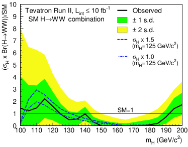
Figure 12: (color online). The best-fit signal cross section expressed as a ratio to the SM cross section as a function of Higgs boson mass from the combination of CDF and D0’s SM Higgs boson searches focusing on the $H\rightarrow W^{+}W^{-}$ decay mode. The dark- and light-shaded bands show the one and two s.d. uncertainty ranges on the fitted signal, respectively. Also shown with blue lines are the median fitted cross sections expected for a SM Higgs boson with $m_{H}=125$ GeV/$c^{2}$ at signal strengths of 1.0 times (short-dashed) and 1.5 times (long-dashed) the SM prediction.

Above 130 GeV/$c^{2}$, the $H\rightarrow W^{+}W^{-}$ channels contribute the majority of the search sensitivity. We combine all $H\to W^{+}W^{-}$ searches from CDF and D0, incorporating potential signal contributions from gluon-gluon fusion, $WH$, $ZH$, and vector boson fusion production. Approximately 75% of the signal comes from the gluon-gluon fusion process, 20% from associated production, and 5% from the VBF process. The LLR distributions are shown in Fig. 11 and the values as a function of Higgs boson mass are listed in Table 6. The data present a one to two s.d. excess in the region from 115 to 140 GeV/$c^{2}$ where there is some separation between the two hypotheses. An excess is also seen in the searches for Higgs bosons with mass $m_{H}>195$ GeV/$c^{2}$, as mentioned in Section VIII.2, but the sensitivity to the SM Higgs boson is not as large at these masses as it is at lower masses. Figure 12 shows the best-fit cross section for the combined $H\rightarrow W^{+}W^{-}$ searches, normalized to the SM prediction, as a function of $m_{H}$, along with the expectations assuming the SM Higgs boson is present at $m_{H}=125$ GeV/$c^{2}$ for signal strengths of 1.0 and 1.5 times the SM prediction.

Table 6: Log-likelihood ratio (LLR) values obtained from the combination of CDF and D0’s Higgs boson search channels focusing on the $H\rightarrow W^{+}W^{-}$ decay mode using the ${\rm CL}_{\rm s}$ method.

$m_{H}$ (GeV/$c^{2}$)	LLRobs	LLRs+b	LLR${}_{b}^{-2\sigma}$	LLR${}_{b}^{-1\sigma}$	LLRb	LLR${}_{b}^{+1\sigma}$	LLR${}_{b}^{+2\sigma}$
100	$-0.42$	$-0.10$	1.36	0.73	0.10	$-0.53$	$-1.16$
105	$-0.72$	$-0.10$	1.34	0.72	0.10	$-0.53$	$-1.15$
110	$-1.07$	$-0.14$	1.62	0.88	0.14	$-0.60$	$-1.34$
115	$-0.80$	$-0.24$	2.18	1.21	0.24	$-0.74$	$-1.71$
120	$-0.98$	$-0.49$	3.26	1.87	0.48	$-0.91$	$-2.30$
125	$-1.69$	$-0.94$	4.73	2.82	0.91	$-1.00$	$-2.91$
130	$-0.59$	$-1.57$	6.44	3.98	1.52	$-0.95$	$-3.41$
135	$-1.11$	$-2.40$	8.36	5.33	2.30	$-0.73$	$-3.77$
140	$-3.38$	$-3.24$	10.09	6.58	3.08	$-0.43$	$-3.94$
145	1.19	$-4.42$	12.23	8.17	4.12	0.06	$-4.00$
150	3.43	$-6.13$	15.01	10.29	5.57	0.85	$-3.87$
155	8.05	$-8.59$	18.45	12.97	7.50	2.02	$-3.46$
160	13.27	$-15.15$	25.92	18.98	12.04	5.10	$-1.84$
165	17.55	$-17.75$	28.69	21.25	13.82	6.38	$-1.05$
170	11.19	$-12.21$	22.80	16.45	10.09	3.74	$-2.61$
175	7.28	$-8.72$	18.44	12.96	7.49	2.02	$-3.46$
180	4.63	$-6.12$	14.80	10.13	5.46	0.78	$-3.89$
185	1.56	$-3.83$	11.05	7.29	3.53	$-0.23$	$-3.99$
190	$-1.39$	$-2.50$	8.51	5.44	2.36	$-0.71$	$-3.79$
195	$-3.24$	$-1.88$	7.12	4.45	1.78	$-0.89$	$-3.56$
200	$-3.23$	$-1.45$	6.08	3.73	1.38	$-0.97$	$-3.32$

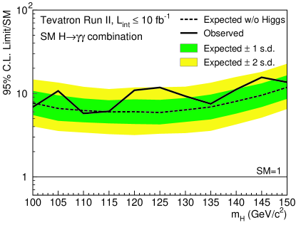
Figure 13: (color online). Observed and median expected (for the background-only hypothesis) 95% C.L. Bayesian upper production limits expressed as multiples of the SM cross section as a function of Higgs boson mass from the combination of CDF and D0’s SM Higgs boson searches focusing on the $H\rightarrow\gamma\gamma$ decay mode. The dark- and light-shaded bands indicate, respectively, the one and two s.d. probability regions in which the limits are expected to fluctuate in the absence of signal.

VIII.5 $H\rightarrow\gamma\gamma$ Decay Mode

We also separately combine CDF and D0’s searches focusing on the $H\rightarrow\gamma\gamma$ decay mode and display the resulting upper limits on the production cross section times the decay branching ratio normalized to the SM prediction in Fig. 13. An excess of approximately two s.d. is seen in these searches at $m_{H}=125$ GeV/$c^{2}$, but its contributions to the fully combined SM cross section and limit are small due to the low expected signal yield in this channel. However, the observed excess in the $H\rightarrow\gamma\gamma$ search channel has a visible impact on Higgs boson coupling constraints as described in Section VIII.7.

VIII.6 $H\rightarrow\tau\tau$ Decay Mode

We also separately combine CDF and D0’s searches focusing on the $H\rightarrow\tau^{+}\tau^{-}$ decay mode and display the resulting upper limits on the production cross section times the decay branching ratio normalized to the SM prediction in Fig. 14.

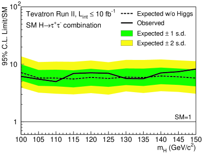
Figure 14: (color online). Observed and median expected (for the background-only hypothesis) 95% C.L. Bayesian upper production limits expressed as multiples of the SM cross section as a function of Higgs boson mass from the combination of CDF and D0’s SM Higgs boson searches focusing on the $H\rightarrow\tau^{+}\tau^{-}$ decay mode. The dark- and light-shaded bands indicate, respectively, the one and two s.d. probability regions in which the limits are expected to fluctuate in the absence of signal.

VIII.7 Compatibility of the Excess with the SM Higgs Boson Hypothesis

The best-fit rate parameters, $R^{\rm{fit}}$, for the full combination of all channels and the combinations of channels focusing on the $H\rightarrow W^{+}W^{-}$, $H\rightarrow b{\bar{b}}$, $H\rightarrow\gamma\gamma$, and $H\rightarrow\tau^{+}\tau^{-}$ decay modes mix are listed in Table 7 as a function of Higgs boson mass over the range 115 $<m_{H}\ <$ 140 GeV/$c^{2}$, where the combined result has sensitivity to a signal and a clear excess exists. For $m_{H}$ = 125 GeV/$c^{2}$, we obtain $R^{\rm{fit}}=1.44^{+0.59}_{-0.56}$ using all decay modes.

Table 7: Best-fit values of $R=(\sigma\times{\cal B})$/SM using the Bayesian method for all SM Higgs boson decay modes combined and the combinations of CDF and D0’s Higgs boson search channels focusing on the $H\rightarrow W^{+}W^{-}$, $H\rightarrow b{\bar{b}}$, $H\rightarrow\gamma\gamma$, and $H\rightarrow\tau^{+}\tau^{-}$ decay modes as a function of Higgs boson mass over the range 115 $<m_{H}<140$ GeV/$c^{2}$. The quoted uncertainties bound the smallest interval containing 68% of the integral of the posterior probability density.

$m_{H}$ (GeV/$c^{2}$)	115	120	125	130	135	140
$R_{\rm{fit}}$(SM)	$0.82^{+0.43}_{-0.46}$	$1.42^{+0.53}_{-0.52}$	$1.44^{+0.59}_{-0.56}$	$1.13^{+0.60}_{-0.60}$	$0.99^{+0.58}_{-0.57}$	$1.15^{+0.57}_{-0.52}$
$R_{\rm{fit}}$($H\rightarrow W^{+}W^{-}$)	$2.22^{+1.65}_{-1.59}$	$1.59^{+1.20}_{-1.15}$	$0.94^{+0.85}_{-0.83}$	$0.49^{+0.69}_{-0.63}$	$0.54^{+0.53}_{-0.52}$	$0.97^{+0.58}_{-0.53}$
$R_{\rm{fit}}$($H\rightarrow b{\bar{b}}$)	$0.72^{+0.47}_{-0.44}$	$1.26^{+0.62}_{-0.55}$	$1.59^{+0.69}_{-0.72}$	$1.82^{+0.91}_{-0.91}$	$2.62^{+1.22}_{-1.21}$	$3.23^{+1.61}_{-1.74}$
$R_{\rm{fit}}$($H\rightarrow\gamma\gamma$)	$0.65^{+2.66}_{-0.54}$	$5.34^{+3.20}_{-2.76}$	$5.97^{+3.39}_{-3.12}$	$3.17^{+2.69}_{-2.81}$	$0.00^{+4.04}_{-0.00}$	$3.31^{+3.30}_{-3.13}$
$R_{\rm{fit}}$($H\rightarrow\tau^{+}\tau^{-}$)	$1.70^{+2.20}_{-1.70}$	$2.00^{+2.22}_{-1.90}$	$1.68^{+2.28}_{-1.68}$	$0.00^{+2.88}_{-0.00}$	$0.00^{+2.83}_{-0.00}$	$1.25^{+2.62}_{-1.15}$

Figure 15 shows the contribution of the four combinations for the different decay modes to the best-fit signal cross section for $m_{H}=125$ GeV/$c^{2}$. The results are consistent with each other, with the full combination, and with the production of the SM Higgs boson at that mass. Figure 16 shows the posterior probability densities obtained for the cross section scale factors from the $H\rightarrow b{\bar{b}}$, $H\rightarrow W^{+}W^{-}$, $H\rightarrow\gamma\gamma$, and $H\rightarrow\tau^{+}\tau^{-}$ combinations.

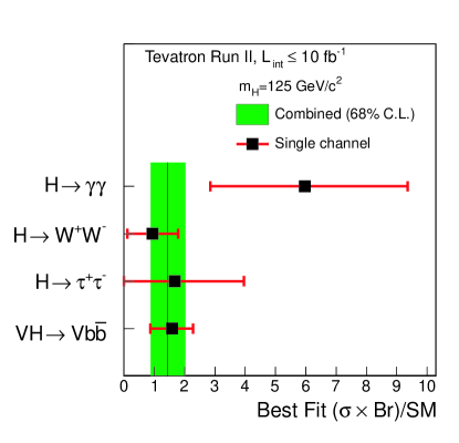
Figure 15: (color online) Best-fit values of $R=(\sigma\times{\cal B})$/SM using the Bayesian method for the combinations of CDF and D0’s Higgs boson search channels focusing on the $H\rightarrow W^{+}W^{-}$, $H\rightarrow b{\bar{b}}$, $H\rightarrow\gamma\gamma$, and $H\rightarrow\tau^{+}\tau^{-}$ decay modes for a Higgs boson mass of 125 GeV/$c^{2}$. The shaded band corresponds to the one s.d. uncertainty on the best-fit value of $R$ for all SM Higgs boson decay modes combined.

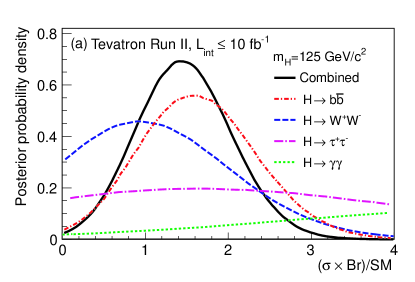
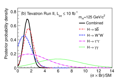
Figure 16: (color online). (a) Posterior probability densities for $R=(\sigma\times{\cal B})$/SM using the Bayesian method from the combinations of CDF and D0’s Higgs boson search channels focusing on the $H\rightarrow W^{+}W^{-}$, $H\rightarrow b{\bar{b}}$, $H\rightarrow\gamma\gamma$, and $H\rightarrow\tau^{+}\tau^{-}$ decay modes and for all SM Higgs boson decay modes combined. The same curves are shown on an expanded scale in (b).

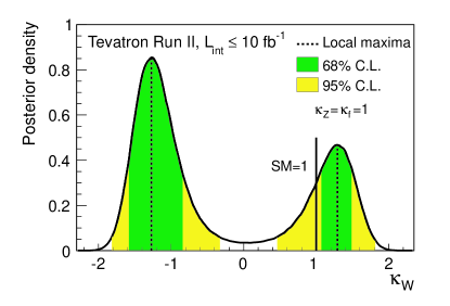
Figure 17: (color online). Posterior probability density for $\kappa_{W}$ from the combination of Tevatron searches for a SM-like Higgs boson with $m_{H}=125$ GeV/$c^{2}$. The couplings of the Higgs boson to fermions and to the $Z$ boson are assumed to be as predicted by the SM. The values that maximize the local posterior probability densities are shown with dashed lines, and the 68% and 95% C.L. intervals are indicated with the dark- and light-shaded regions, respectively. The predicted SM value of $\kappa_{W}$ is indicated by the solid vertical line.

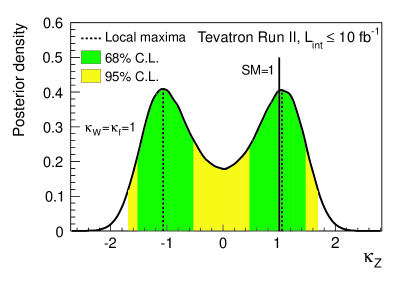
Figure 18: (color online). Posterior probability density for $\kappa_{Z}$ from the combination of Tevatron searches for a SM-like Higgs boson with $m_{H}=125$ GeV/$c^{2}$. The couplings of the Higgs boson to fermions and to the $W^{\pm}$ boson are assumed to be as predicted by the SM. The values that maximize the local posterior probability densities are shown with dashed lines, and the 68% and 95% C.L. intervals are indicated with the dark- and light-shaded regions, respectively. The predicted SM value of $\kappa_{Z}$ is indicated by the solid vertical line.

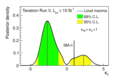
Figure 19: (color online). Posterior probability density for $\kappa_{f}$ from the combination of Tevatron searches for a SM-like Higgs boson with $m_{H}=125$ GeV/$c^{2}$. The couplings of the Higgs boson to the $W^{\pm}$ and $Z$ bosons are assumed to be as predicted by the SM. The values that maximize the local posterior probability densities are shown with dashed lines, and the 68% and 95% C.L. intervals are indicated with the dark- and light-shaded regions, respectively. The predicted SM value of $\kappa_{f}$ is indicated by the solid vertical line.

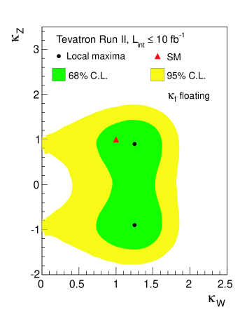
Figure 20: (color online). Two-dimensional constraints in the $(\kappa_{W},\kappa_{Z})$ plane, for the combined Tevatron searches for a SM-like Higgs boson with mass 125 GeV/$c^{2}$ allowing $\kappa_{f}$ to float. The points that maximize the local posterior probability densities are marked with dots, and the 68% and 95% C.L. intervals are indicated with the dark- and light-shaded regions, respectively. The SM prediction for $(\kappa_{W},\kappa_{Z})$ is marked with a triangle.

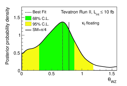
Figure 21: (color online). Posterior probability density for $\theta_{\it WZ}={\rm{tan}}^{-1}(\kappa_{Z}/\kappa_{W})$, from the combination of Tevatron searches for a SM-like Higgs boson with $m_{H}=125$ GeV/$c^{2}$ allowing $\kappa_{f}$ to float. The value that maximizes the posterior probability density is shown with a dashed vertical line, and the 68% and 95% C.L. intervals are indicated with the dark- and light-shaded regions, respectively. The predicted SM value of $\theta_{\it WZ}$ is indicated by the solid vertical line.

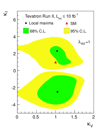
Figure 22: (color online). Two-dimensional constraints in the $(\kappa_{V},\kappa_{f})$ plane, for the combined Tevatron searches for a SM-like Higgs boson with mass 125 GeV/$c^{2}$ assuming Custodial symmetry ($\lambda_{\it WZ}=1$). The points that maximize the local posterior probability densities are marked with dots, and the 68% and 95% C.L. intervals are indicated with the dark- and light-shaded regions, respectively. The SM prediction for $(\kappa_{V},\kappa_{f})$ is marked with a triangle.

The Higgs boson is expected to couple more strongly to more massive particles than to less massive ones, and thus may provide sensitivity to non-SM particles whose interactions become more relevant at higher energies. It is important therefore to study in detail the properties of the new particle. The channel-by-channel values of $R=(\sigma\times{\cal B})$/SM provide useful constraints on the possible couplings of the particle grojean , but their interpretation is ambiguous because signal contributions from multiple sources are simultaneously accepted by each sub-channel. For example, the $ZH\rightarrow\nu{\bar{\nu}}b{\bar{b}}$ channels have sensitivity to both the $WH$ and $ZH$ production modes, and the $H\rightarrow W^{+}W^{-}$ searches are sensitive to gluon-gluon fusion, $WH$, $ZH$, and VBF in different mixtures within independent sub-channels characterized by the number of reconstructed jets.

Most of the searches conducted at the Tevatron are sensitive to the product of fermion and boson coupling strengths. In the $VH\rightarrow Vb{\bar{b}}$ searches, the production depends on the coupling of the Higgs boson to the weak vector bosons, while the decay is to fermions. In the $gg\rightarrow H\rightarrow W^{+}W^{-}$ searches, the production is dominated by the Higgs boson couplings to fermions via the quark loop processes, but the decay is to bosons. A large enhancement of the Higgs boson’s couplings to fermions can thus be masked by a small coupling to bosons, and vice versa, as shown in Fig. 2 of Ref. grojean . However, other less-sensitive channels included in this combination provide additional constraints. The same-sign di-lepton searches, the tri-lepton searches, and some of the searches with tau leptons as decay products of $W$ bosons are primarily sensitive to $VH\rightarrow VW^{+}W^{-}$, an entirely bosonic process, although their results are customarily reported in combination with the other $H\rightarrow W^{+}W^{-}$ searches. The searches for $t{\bar{t}}H\rightarrow t{\bar{t}}b{\bar{b}}$ provide constraints on the fermion couplings with minimal masking from the bosonic couplings.

We follow the notation of Ref. lhccouplingrec and introduce multiplicative scaling factors for the coupling of the Higgs boson to fermions ($\kappa_{f}$) and either to $W$ bosons ($\kappa_{W}$) and $Z$ bosons ($\kappa_{Z}$) or more generically to vector bosons ($\kappa_{V}$). We then search for deviations from the expected SM values of $\kappa_{i}=1$.

The first test assumes $m_{H}=125$ GeV/$c^{2}$, based on the ATLAS and CMS observations, and fits for the $H\rightarrow W^{+}W^{-}$ coupling, holding all other couplings fixed to their SM values. This test corresponds to holding the values of $\kappa_{Z}=\kappa_{f}=1$, while varying $\kappa_{W}$. At each value of $\kappa_{W}$, we recompute the predicted cross sections and decay branching ratios, as described in Ref. lhccouplingrec . We assume a uniform prior density in $\kappa_{W}$, and show the posterior probability distribution in Fig. 17. A negative sign of $\kappa_{W}$ is preferred by the Tevatron data due to the excess seen in the $H\rightarrow\gamma\gamma$ searches. In the SM, this process proceeds at lowest order via a $W$-boson loop or a quark loop (dominated by the top quark), with destructive interference between the two contributions spira95 , as given by $\Gamma(H\rightarrow\gamma\gamma)=\Gamma(H\rightarrow\gamma\gamma)_{SM}\times|1.28~{}\kappa_{V}-0.28~{}\kappa_{f}|^{2}$. If the sign of the $H\rightarrow W^{+}W^{-}$ coupling is negative, then this interference becomes constructive, allowing for a larger prediction of the yield. We obtain a best-fit value of $\kappa_{W}=-1.27$. Our procedure for finding the smallest set of intervals that contain 68% of the integral of the posterior results in two intervals, $-1.56<\kappa_{W}<-0.81$ and $1.04<\kappa_{W}<1.51$. We perform a similar test for $\kappa_{Z}$, assuming $\kappa_{W}=\kappa_{f}=1$. The resulting posterior probability density is shown in Fig. 18. The Higgs boson searches at the Tevatron are sensitive almost exclusively to the square of $\kappa_{Z}$, and thus the posterior density is nearly symmetric in positive and negative couplings. The best-fit values are $\kappa_{Z}=1.05_{-0.55}^{+0.45}$ and $\kappa_{Z}=-1.05_{-0.45}^{+0.55}$. Finally, we perform a similar test for $\kappa_{f}$, the common scale factor on the Higgs boson couplings to fermions, holding $\kappa_{W}=\kappa_{Z}=1$. The resulting posterior probability density is shown in Fig. 19. An asymmetry is seen in this distribution, due again to the outcome in the $H\rightarrow\gamma\gamma$ channels. We obtain a best-fit value of $\kappa_{f}=-2.64_{-1.30}^{+1.59}$. The large magnitude of the fitted value is due to the excesses seen in the $H\rightarrow b{\bar{b}}$ and $H\rightarrow\gamma\gamma$ searches.

We then allow both $\kappa_{W}$ and $\kappa_{Z}$ to vary independently, also allowing $\kappa_{f}$ to vary by integrating the likelihood function times a uniform prior in $\kappa_{f}$ over negative and positive values. The resulting areas in the $(\kappa_{W},\kappa_{Z})$ plane preferred by the Tevatron data are shown in Fig. 20. While we allow either coupling scale factor to be negative, only two quadrants are shown in Fig. 20 due to an overall sign ambiguity. The point $(\kappa_{W},\kappa_{Z})=(0,0)$ corresponds to no Higgs boson production or decay in the most sensitive search modes at the Tevatron and is excluded at more than the 95% C.L. due to the Higgs-boson-like signal in the $H\rightarrow b\bar{b}$ and $H\rightarrow W^{+}W^{-}$ channels. Our best-fit points are $(\kappa_{W},\kappa_{Z})=(1.25,\pm 0.90)$.

We study the ratio $\lambda_{\it WZ}=\kappa_{W}/\kappa_{Z}$ using the same posterior probability density that is used in Fig. 20. We choose a projection onto a one dimensional variable that preserves the uniformity of the prior probability density in the two-dimensional plane. This variable is the angle with respect to the $\kappa_{W}$ axis, $\theta_{\it WZ}={\rm{tan}}^{-1}(\kappa_{Z}/\kappa_{W})={\rm{tan}}^{-1}(1/\lambda_{\it WZ})$. Figure 21 shows the one-dimensional posterior probability density in this variable. This function is symmetric for positive and negative $\theta_{\it WZ}$. We measure $|\theta_{\it WZ}|=0.68_{-0.41}^{+0.21}$, which corresponds to $\lambda_{\it WZ}=1.24^{+2.34}_{-0.42}$.

Assuming that custodial symmetry custodial holds ($\lambda_{\it WZ}=1$), we allow both $\kappa_{V}$ and $\kappa_{f}$ to vary, and show in Fig. 22 the regions preferred at the 68% C.L. and the 95% C.L. in the two-dimensional plane $(\kappa_{V},\kappa_{f})$. The asymmetry induced by the excesses in the $H\rightarrow\gamma\gamma$ searches is visible in this projection as well. The best-fit point is $(\kappa_{V},\kappa_{f})=(1.05,-2.40)$, but a secondary maximum in the posterior density is seen at $(\kappa_{V},\kappa_{f})=(1.05,2.30)$, consistent with the SM expectation, given the large uncertainties. The integral of the posterior density in the (+,+) quadrant is 26% of the total, while the remaining 74% of the integral of the posterior density is contained within the (+,–) quadrant.

IX Results - Non-standard model interpretations

The mechanism of electroweak symmetry breaking may entail a richer phenomenology than expected in the SM. Natural extensions include the addition of a fourth generation of fermions with masses much larger than those of the three known generations or models with several Higgs bosons or models in which the Higgs boson(s) may have modified couplings. We interpret our Higgs boson search results in models with a sequential fourth generation of fermions (SM4) and in the fermiophobic Higgs model (FHM) described below.

IX.1 Fourth Generation Interpretation

With the inclusion of two additional heavy fourth-generation quarks in the SM4 fourthgen , the $gg\rightarrow H$ coupling is enhanced by a factor of roughly three relative to the SM coupling arik ; g4_hdecay ; abf . The partial decay width for $H\rightarrow gg$ is enhanced by the same factor as the production cross section. However, because the $H\rightarrow gg$ decay is mediated by a loop amplitude, the $H\rightarrow W^{+}W^{-}$ decay continues to dominate for Higgs boson masses above 135 GeV/$c^{2}$. Since the expected signal yield is larger in the SM4 model than the SM, the sensitivity of CDF and D0’s Higgs boson searches extends to higher masses. For this reason, the upper end of the search range for the relevant channels is raised to 300 GeV/$c^{2}$ for interpretations associated with this model.

Two scenarios for the masses of the fourth-generation fermions are considered. In the first, the low-mass scenario, we set the mass of the fourth-generation neutrino $m_{\nu 4}=80$ GeV/$c^{2}$ and the mass of the fourth-generation charged lepton $m_{\ell 4}=100$ GeV/$c^{2}$, in order to have the maximum impact on the Higgs boson decay branching ratios and to be compatible with the experimental constraint on the mass of an unstable $\nu_{4}$ L3_lepton . In the case that the $\nu_{4}$ is stable or has a lifetime long enough to escape the search presented in Ref. L3_lepton , $m_{\nu_{4}}$ could be lighter, modifying the decay branching ratios belotsky , resulting in weaker mass limits. In our second scenario, the high-mass scenario, we set $m_{\nu 4}=m_{\ell 4}=1$ TeV/$c^{2}$, so that the fourth-generation leptons do not modify the decay branching ratios of the Higgs boson relative to the SM. In both scenarios, we choose the masses of the quarks to be those of the second scenario in Ref. abf ($m_{d4}$ = 400 GeV/$c^{2}$ and $m_{u4}$ = 450 GeV/$c^{2}$). The next-to-next-to-leading order (NNLO) production cross section calculation of Ref. abf is used, which is a modified version of the NNLO SM calculation. Previous interpretations of SM Higgs boson searches within the context of a fourth generation of fermions at the Tevatron excluded $131<m_{H}<207$ GeV/$c^{2}$ PRDRC . Similar searches have been performed by the ATLAS atlas4g and CMS cms4g Collaborations, excluding $140<m_{H}<185$ GeV/$c^{2}$ and $144<m_{H}<207$ GeV/$c^{2}$, respectively. A more recent search by the CMS Collaboration excluded the mass range $110<m_{H}<600$ GeV/$c^{2}$ cms4g-new .

We combine our searches for a Higgs boson in the processes $gg\rightarrow H\rightarrow W^{+}W^{-}$ and $gg\rightarrow H\rightarrow ZZ$. Limits on the SM4 models and on $\sigma(gg\rightarrow H)\times\mathcal{B}(H\rightarrow W^{+}W^{-})$ are derived. This result is an update of Ref. PRDRC . The analyses are performed equivalently to the SM searches except that $gg\rightarrow H$ production only is considered for the signal. The MVA classifiers are retrained accordingly and, for the specific case of the D0 $H\rightarrow W^{+}W^{-}\rightarrow\ell^{\pm}\nu\ell^{\mp}\nu$ channel, the two-jet bin, which is less sensitive to $gg\rightarrow H$ production, is not included.

The branching ratios for $H\rightarrow W^{+}W^{-}$ are calculated using hdecay hde modified to include fourth-generation fermions g4_hdecay . To include the $gg\rightarrow H\rightarrow ZZ$ searches, we assume the SM value for $\mathcal{B}(H\rightarrow W^{+}W^{-})/\mathcal{B}(H\rightarrow ZZ)$. In setting limits on $\sigma(gg\rightarrow H)\times\mathcal{B}(H\rightarrow W^{+}W^{-})$, the $gg\rightarrow H\rightarrow ZZ$ process is included assuming that its signal yield scales equivalently to that from the $gg\rightarrow H\rightarrow W^{+}W^{-}$ channel.

When setting limits on $\sigma(gg\rightarrow H)\times\mathcal{B}(H\rightarrow W^{+}W^{-})$, the theoretical uncertainty on the prediction of $\sigma(gg\rightarrow H)\times\mathcal{B}(H\rightarrow W^{+}W^{-})$ is not included since these limits are independent of the predictions. However, when setting limits on $m_{H}$ in the context of fourth-generation models, uncertainties on the theoretical predictions are included as described for the SM searches.

The combined limits on $\sigma(gg\rightarrow H)\times\mathcal{B}(H\rightarrow W^{+}W^{-})$ obtained using the Bayesian method are shown in Fig. 23 along with the theory predictions for fourth-generation models in the low- and high-mass scenarios. Limits obtained using both the Bayesian and ${\rm CL}_{\rm s}$ methods are listed as a function of Higgs boson mass in Table 8. A broad, moderate excess above the background expectation is seen for masses above 200 GeV/$c^{2}$.

Production limits obtained for the two SM4 scenarios using the Bayesian method are shown in Fig. 24. The limits are presented as ratios relative to SM4 low-mass scenario predictions as a function of the Higgs boson mass. In the low-mass scenario, which gives the smaller excluded mass range, a SM-like Higgs boson with a mass in the range 121–225 GeV/$c^{2}$ is excluded at the 95% C.L. The expected excluded mass range is 118–270 GeV/$c^{2}$. In the high-mass scenario, the mass range 121–232 GeV/$c^{2}$ is excluded, with an expected excluded mass range of 118–290 GeV/$c^{2}$.

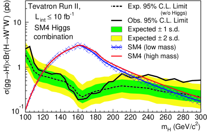
Figure 23: (color online). Observed and median expected (for the background-only hypothesis) 95% C.L. Bayesian upper limits on the cross section times branching ratio $\sigma(gg\rightarrow H)\times\mathcal{B}(H\rightarrow W^{+}W^{-})$ from the combination of CDF and D0’s Higgs boson search channels focusing on this production and decay mode. The dark and light-shaded bands indicate, respectively, the one and two s.d. probability regions in which the limits are expected to fluctuate in the absence of signal. Theoretical predictions for SM4 in the low- and high-mass scenarios are shown with blue and red lines, respectively. The hatched band indicates the theoretical uncertainty associated with the SM4 low-mass scenario.

Table 8: Observed and median expected (for the background-only hypothesis) 95% C.L. upper limits on the cross section times branching ratio $\sigma(gg\rightarrow H)\times\mathcal{B}(H\rightarrow W^{+}W^{-})$ from the combination of CDF and D0’s Higgs boson search channels focusing on this production and decay mode, obtained using the Bayesian and ${\rm CL}_{\rm s}$ methods.

	Bayesian		${\rm CL}_{\rm s}$
$m_{H}$	Observed	Expected	Observed	Expected
(GeV/$c^{2}$)	limit (pb)	limit (pb)	limit (pb)	limit (pb)
100	2.56	1.89	2.58	1.87
105	2.87	1.33	2.62	1.32
110	1.24	0.81	1.27	0.82
115	0.88	0.68	0.90	0.70
120	0.81	0.63	0.81	0.66
125	0.75	0.61	0.77	0.61
130	0.70	0.57	0.70	0.58
135	0.72	0.53	0.75	0.54
140	0.70	0.50	0.72	0.52
145	0.56	0.48	0.55	0.48
150	0.33	0.40	0.32	0.42
155	0.28	0.34	0.30	0.35
160	0.19	0.25	0.20	0.26
165	0.19	0.22	0.20	0.22
170	0.20	0.24	0.21	0.25
175	0.26	0.27	0.26	0.27
180	0.26	0.29	0.26	0.29
185	0.28	0.31	0.29	0.31
190	0.38	0.32	0.40	0.33
195	0.47	0.33	0.47	0.34
200	0.48	0.36	0.49	0.37
210	0.71	0.38	0.73	0.39
220	0.59	0.37	0.60	0.37
230	0.60	0.36	0.61	0.36
240	0.69	0.34	0.69	0.34
250	0.61	0.30	0.60	0.30
260	0.51	0.28	0.49	0.29
270	0.55	0.27	0.56	0.27
280	0.46	0.25	0.47	0.25
290	0.50	0.24	0.48	0.24
300	0.52	0.22	0.50	0.22

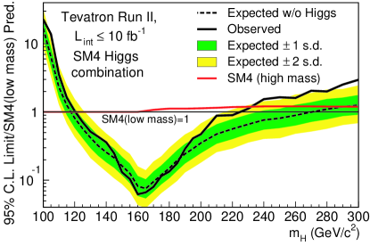
Figure 24: (color online). Observed and median expected (for the background-only hypothesis) 95% C.L. Bayesian upper production limits expressed as multiples of the SM4 (low-mass scenario) cross section as a function of Higgs boson mass from the combination of CDF and D0’s Higgs boson searches focusing on the $gg\rightarrow H$ production and $H\rightarrow W^{+}W^{-}$ decay modes. Uncertainties associated with theoretical cross section and branching ratio predictions are incorporated in the limit. The dark and light-shaded bands indicate, respectively, the one and two s.d. probability regions in which the limits are expected to fluctuate in the absence of signal. The red line shows the prediction for the signal rate in the high-mass scenario, divided by that of the low-mass scenario.

IX.2 Fermiophobic Interpretation

In the FHM, the lightest Higgs boson does not couple to fermions at tree level, but aside from this one difference, its behavior is indistinguishable from that of the SM Higgs boson. In the FHM, the production of Higgs bosons, $H_{f}$, at hadron colliders via the process $gg\rightarrow H_{f}$ is suppressed to a negligible rate and is ignored in the context of this interpretation. The associated production mechanisms $p{\bar{p}}\rightarrow WH_{f}+X$ and $p{\bar{p}}\rightarrow ZH_{f}+X$, as well as the vector-boson-fusion (VBF) processes $q\bar{q}\rightarrow q^{\prime}\bar{q}^{\prime}H_{f}$, remain nearly unchanged relative to the corresponding processes in the SM. Thus, the corresponding SM cross sections and associated uncertainties described previously are also used here. In the FHM, direct decays to fermions are forbidden; the decays to $W^{+}W^{-}$, $\gamma\gamma$, $ZZ$, and $Z\gamma$ account for nearly the entire decay width. For the mass range under investigation the $W^{+}W^{-}$ decay mode has the largest branching fraction. The branching fraction ${\cal{B}}(H_{f}\rightarrow\gamma\gamma$) is greatly enhanced over ${\cal{B}}(H_{\rm{SM}}\rightarrow\gamma\gamma$) for all $m_{H}$, and the clean signature and excellent mass resolution of this channel provide most of the search sensitivity for $m_{H_{f}}<120$ GeV/$c^{2}$. The analyses combined here seek Higgs boson decays to $W^{+}W^{-}$, $\gamma\gamma$, and $ZZ$. Previous searches for a fermiophobic Higgs boson at the Tevatron excluded signals with masses smaller than 119 GeV/$c^{2}$ prevtevfhm ; the expected exclusion was also $m_{H_{f}}<119$ GeV/$c^{2}$. The ATLAS and CMS Collaborations excluded $m_{H_{f}}$ in the ranges 110.0–118.0 GeV/$c^{2}$ and 119.5–121.0 GeV/$c^{2}$ using diphoton final states atlasfhm and in the range 110–194 GeV/$c^{2}$ by combining multiple final states cmsfhm .

The SM $H\rightarrow\gamma\gamma$ analyses are reoptimized as the kinematic distributions of the Higgs bosons, their decay products, and the particles produced in association with the Higgs bosons differ between the FHM and the SM. Events contain either an associated $W$ or $Z$ boson, or recoiling quark jets in the case of VBF and thus the transverse momentum ($p_{T}$) of the Higgs boson is on average greater than it is in the SM. The analyses combined here update previous searches for the Higgs boson in the FHM prevcdffhm ; prevd0fhm . Similarly, SM searches in $H\rightarrow W^{+}W^{-}$ channels cannot be interpreted directly in the FHM due to the different mixture of production modes. Signal contributions from $gg\rightarrow H_{f}$ production to the MVA discriminant distributions are ignored, and the remaining contributions from other production mechanisms are scaled by the ratio of branching ratio predictions ${\cal{B}}(H_{f}\rightarrow VV)/{\cal{B}}(H_{\rm{SM}}\rightarrow VV)$. The existing subdivision of channels based on the number of reconstructed jets accompanying the leptons and missing transverse energy in the event naturally optimizes the search within the FHM interpretation. Hence, the development of a separate set of analysis channels as in the case of $H_{f}\rightarrow\gamma\gamma$ is not required, though the MVAs are retrained.

The combined limits on Higgs boson production normalized to FHM predictions obtained from both the Bayesian and CL_s methods are listed in Table 9 as a function of Higgs boson mass. The expected limits assume no Higgs boson production. The limits obtained using the Bayesian method are shown in Fig. 25. Fermiophobic Higgs bosons in the mass range 100–116 GeV/$c^{2}$ are excluded at the 95% C.L.; the expected excluded mass range is 100–135 GeV/$c^{2}$.

Table 9: Ratios of observed and median expected (for the background-only hypothesis) 95% C.L. upper limits on the production rate of a Fermiophobic Higgs boson relative to the FHM prediction as a function of the Higgs boson mass for the combination of CDF and D0’s searches, obtained using the Bayesian and ${\rm CL}_{\rm s}$ methods.

	Bayesian		${\rm CL}_{\rm s}$
$m_{H_{f}}$ (GeV/$c^{2}$)	$R_{95}^{\mathrm{obs}}$	$R_{95}^{\mathrm{exp}}$	$R_{95}^{\mathrm{obs}}$	$R_{95}^{\mathrm{exp}}$
100	0.21	0.13	0.21	0.13
105	0.36	0.22	0.37	0.23
110	0.40	0.37	0.36	0.37
115	0.95	0.54	0.88	0.53
120	1.13	0.69	1.06	0.68
125	1.41	0.83	1.44	0.81
130	1.21	0.91	1.06	0.90
135	1.26	1.00	1.16	0.97
140	1.65	1.11	1.48	1.06
145	1.47	1.15	1.30	1.13
150	1.33	1.21	1.19	1.17
155	1.30	1.19	1.17	1.18
160	1.20	1.17	1.11	1.14
165	0.98	1.17	0.94	1.11
170	1.49	1.31	1.35	1.26
175	1.96	1.48	1.76	1.43
180	2.34	1.72	2.04	1.60
185	3.13	1.96	2.58	1.93
190	3.75	2.36	3.24	2.32
195	4.58	2.62	3.92	2.54
200	5.43	2.85	4.64	2.77

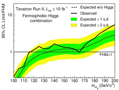
Figure 25: (color online). Observed and median expected (for the background-only hypothesis) 95% C.L. Bayesian upper production limits expressed as multiples of the FHM cross section as a function of Higgs boson mass for the combined CDF and D0 searches. The dark and light-shaded bands indicate, respectively, the one and two s.d. probability regions in which the limits are expected to fluctuate in the absence of signal.

X Conclusions

The search for the standard model Higgs boson at the Tevatron is challenging due to the small expected signal and the need to accurately model large background contributions. We have developed advanced tools to search for the Higgs boson in the leading production and decay modes predicted by the SM and control the impact of systematic uncertainties using constraints from the observed data. We have combined searches by the CDF and D0 Collaborations for the standard model Higgs boson in the mass range 90–200 GeV$/c^{2}$ using Tevatron $p{\bar{p}}$ collision data corresponding to up to 10 fb^-1 of integrated luminosity collected at $\sqrt{s}=1.96$ TeV. The results of searches focusing on the $H\rightarrow b{\bar{b}}$, $H\rightarrow W^{+}W^{-}$, $H\rightarrow ZZ$, $H\rightarrow\tau^{+}\tau^{-}$, and $H\rightarrow\gamma\gamma$ decay modes are included in the combination. The results are also interpreted in fermiophobic and fourth generation models. Fermiophobic Higgs bosons in the mass range 100–116 GeV/$c^{2}$ are excluded at the 95% C.L., and a SM-like Higgs boson in the presence of a fourth sequential generation of fermions is excluded in the mass range 121–225 GeV/$c^{2}$ at the 95% C.L. The SM Higgs boson is excluded, at the 95% C.L., from 90 to 109 GeV/$c^{2}$, and from 149 to 182 GeV/$c^{2}$. The expected exclusion regions in the absence of signal are 90–120 GeV/$c^{2}$ and 140–184 GeV/$c^{2}$. The results of the $H\to b\bar{b}$ searches were validated through a measurement of the diboson ($WZ+ZZ$) production cross section using the same data samples and analysis techniques, treating those diboson processes as signal. The resulting diboson cross-section measurement is in agreement with the SM prediction. We observe a significant excess of events in the mass range between 115 and 140 GeV/$c^{2}$. The local significance at $m_{H}=125$ GeV/$c^{2}$ corresponds to 3.0 standard deviations, with a median expected significance, assuming the SM Higgs boson is present at $m_{H}=125$ GeV/$c^{2}$, of 1.9 standard deviations. with a best-fit signal strength of $1.44^{+0.59}_{-0.56}$ times the SM expectation. We also separately combined searches focusing on the $H\to b\bar{b}$, $H\to W^{+}W^{-}$, $H\rightarrow\tau^{+}\tau^{-}$, and $H\rightarrow\gamma\gamma$ decay modes. The observed best-fit signal strengths obtained from each of these combinations are consistent with the expectations for a SM Higgs boson at $m_{H}=125$ GeV/$c^{2}$. We performed tests of the compatibility of the observed excess with the expectations for the couplings of a SM Higgs boson and saw no significant deviations.

XI ACKNOWLEDGMENTS

We thank the Fermilab staff and technical staffs of the participating institutions for their vital contributions. We acknowledge support from the DOE and NSF (USA), ARC (Australia), CNPq, FAPERJ, FAPESP and FUNDUNESP (Brazil), NSERC (Canada), NSC, CAS and CNSF (China), Colciencias (Colombia), MSMT and GACR (Czech Republic), the Academy of Finland, CEA and CNRS/IN2P3 (France), BMBF and DFG (Germany), DAE and DST (India), SFI (Ireland), INFN (Italy), MEXT (Japan), the Korean World Class University Program and NRF (Korea), CONACyT (Mexico), FOM (Netherlands), MON, NRC KI and RFBR (Russia), the Slovak R&D Agency, the Ministerio de Ciencia e Innovación, and Programa Consolider-Ingenio 2010 (Spain), The Swedish Research Council (Sweden), SNSF (Switzerland), STFC and the Royal Society (United Kingdom), the A.P. Sloan Foundation (USA), and the EU community Marie Curie Fellowship contract 302103.

References

- (1) S. L. Glashow, Nucl. Phys. 22, 579 (1961); S. Weinberg, Phys. Rev. Lett. 19, 1264 (1967); A. Salam, Elementary Particle Theory, ed. N. Svartholm (Almqvist & Wiksell, Stockholm), 367 (1968).
- (2) F. Englert and R. Brout, Phys. Rev. Lett. 13, 321 (1964); P. W. Higgs, Phys. Rev. Lett. 13, 508 (1964); G. S. Guralnik, C. R. Hagen, and T. W. B. Kibble, Phys. Rev. Lett. 13, 585 (1964); P. W. Higgs, Phys. Rev. 145, 1156 (1966).
- (3) T. Aaltonen et al. (CDF and D0 Collaborations), arXiv:1204.0042 (2012).
- (4) T. Aaltonen et al. (CDF and D0 Collaborations), Phys. Rev. D 86, 092003 (2012).
- (5) The ALEPH, CDF, D0, DELPHI, L3, OPAL, and SLD Collaborations, the LEP Electroweak Working Group, the Tevatron Electroweak Working Group, and the SLD Electroweak and Heavy Flavour Working Groups, arXiv:1012.2367v2 (2011). The most recent values from March 2012, as quoted, are available from http://lepewwg.web.cern.ch/LEPEWWG/.
- (6) In this article, C.L. denotes confidence level for frequentist and modified frequentist results, and credibility level for Bayesian results.
- (7) The ALEPH, DELPHI, L3 and OPAL Collaborations, and the LEP Working Group for Higgs Boson Searches, Phys. Lett. B 565, 61 (2003).
- (8) G. Aad et al. (ATLAS Collaboration), Phys. Lett. B 716, 1 (2012).
- (9) S. Chatrchyan et al. (CMS Collaboration), Phys. Lett. B 716, 30 (2012).
- atl (a) G. Aad et al. (ATLAS Collaboration), Phys. Lett. B 718, 369 (2012).
- cms (a) S. Chatrchyan et al. (CMS Collaboration), Phys. Lett. B 710, 284 (2012).
- (12) T. Aaltonen et al. (CDF and D0 Collaborations), Phys. Rev. Lett. 109, 071804 (2012).
- tev (b) T. Aaltonen et al. (CDF and D0 Collaborations), Phys. Rev. Lett. 104, 061802 (2010).
- (14) T. Aaltonen et al. (CDF Collaboration), arXiv:1301.6668 (2013), accepted by Phys. Rev. D.
- (15) V. M. Abazov et al. (D0 Collaboration), arXiv:1303.0823 (2013), accepted by Phys. Rev. D.
- (16) T. Sjöstrand, S. Mrenna, and P. Skands, J. High Energy Phys. 05 (2006) 026. We use pythia version 6.216 to generate the Higgs boson signals.
-
(17)
H. L. Lai et al., Eur. Phys. J. C 12, 375 (2000);
J. Pumplin et al., J. High Energy Phys. 07 (2002) 012. - (18) C. Anastasiou, R. Boughezal, and F. Petriello, J. High Energy Phys. 04 (2009) 003.
- (19) D. de Florian and M. Grazzini, Phys. Lett. B 674, 291 (2009).
- (20) J. Baglio and A. Djouadi, J. High Energy Phys. 10 (2010) 064; O. Brein, R. V. Harlander, M. Weisemann, and T. Zirke, Eur. Phys. J. C 72, 1868 (2012).
- (21) P. Bolzoni, F. Maltoni, S.-O. Moch, and M. Zaro, Phys. Rev. Lett. 105, 011801 (2010).
- (22) M. Ciccolini, A. Denner, and S. Dittmaier, Phys. Rev. Lett. 99, 161803 (2007); Phys. Rev. D 77, 013002 (2008).
-
(23)
W. Beenakker, S. Dittmaier, M. Krämer, B. Plümper,
M. Spira, and P. M. Zerwas, Phys. Rev. Lett. 87, 201805 (2001);
L. Reina and S. Dawson, Phys. Rev. Lett. 87, 201804 (2001). - (24) A. D. Martin, W. J. Stirling, R. S. Thorne, and G. Watt, Eur. Phys. J. C 63, 189 (2009).
- lhc (a) S. Dittmaier et al. (LHC Higgs Cross Section Working Group), arXiv:1201.3084 (2012).
- (26) A. Djouadi, J. Kalinowski, and M. Spira, Comput. Phys. Commun. 108, 56 (1998). We use hdecay Version 3.53.
- (27) A. Bredenstein, A. Denner, S. Dittmaier, and M. M. Weber, Phys. Rev. D 74, 013004 (2006); A. Bredenstein, A. Denner, S. Dittmaier, A. Mück, and M. M. Weber, J. High Energy Phys. 02 (2007) 080.
- (28) G. Bozzi, S. Catani, D. de Florian, and M. Grazzini, Phys. Lett. B 564, 65 (2003); Nucl. Phys. B737, 73 (2006).
- (29) M. Mangano, M. Moretti, F. Piccinini, R. Pittau, and A. Polosa, J. High Energy Phys. 07 (2003) 001.
- (30) S. Frixione and B.R. Webber, J. High Energy Phys. 06 (2002) 029.
- (31) G. Corcella, I. G. Knowles, G. Marchesini, S. Moretti, K. Odagiri, P. Richardson, M. H. Seymour, and B. R. Webber, J. High Energy Phys. 01 (2001) 010.
- (32) E. Boos, V. Bunichev, M. Dubinin, L. Dudko, V. Ilyin, A. Kryukov, V. Edneral, V. Savrin, A. Semenov, and A. Sherstnev, Nucl. Instrum. Methods Phys. Res., Sect. A 534, 250 (2004); E. E. Boos, V. E. Bunichev, L. V. Dudko, V. I. Savrin, and A. V. Sherstnev, Phys. Atom. Nucl. 69, 1317 (2006).
- (33) J. M. Campbell and R. K. Ellis, Phys. Rev. D 60, 113006 (1999).
- (34) U. Langenfeld, S. Moch, and P. Uwer, Phys. Rev. D 80, 054009 (2009).
- (35) N. Kidonakis, Phys. Rev. D 74, 114012 (2006).
- (36) R. Hamberg, W. L. van Neerven, and T. Matsuura, Nucl. Phys. B359, 343 (1991) [Erratum-ibid. B644, 403 (2002)].
- (37) A heavy-flavor jet is a reconstructed cluster of calorimeter energies associated with particles produced in the hadronization and decay of a bottom or charm quark.
- (38) A -tagged jet is one identified to have originated from the decay of a heavy flavor quark.
- (39) R. Brun and F. Carminati, CERN Program Library Long Writeup W5013, 1993 (unpublished).
- cdf (e) D. Acosta et al. (CDF Collaboration), Phys. Rev. D 71, 032001 (2005); A. Abulencia et al. (CDF Collaboration), J. Phys. G Nucl. Part. Phys. 34, 2457 (2007).
- (41) V. M. Abazov et al. (D0 Collaboration), Nucl. Instrum. Methods Phys. Res., Sect. A 565, 463 (2006); M. Abolins et al., Nucl. Instrum. Methods Phys. Res., Sect. A 584, 75 (2008); R. Angstadt et al., Nucl. Instrum. Methods Phys. Res., Sect. A 622, 298 (2010).
- (42) For a recent review, see P. C. Bhat, Ann. Rev. Nucl. Part. Sci. 61, 281 (2011). The specific details of the MVA for each analysis are described in the respective references.
- (43) J. Freeman et al., Nucl. Instrum. Methods Phys. Res., Sect. A 697, 64 (2013); D. Acosta et al. (CDF Collaboration), Phys. Rev. D 71, 052003 (2005); A. Abulencia et al. (CDF Collaboration), Phys. Rev. D 74, 072006 (2006).
- (44) V. M. Abazov et al., Nucl. Instrum. Methods Phys. Res., Sect. A 620, 490 (2010).
- (45) V. M. Abazov et al. (D0 Collaboration), Phys. Lett. B 716, 285 (2012).
- (46) Statistics in K. Nakamura et al. (Particle Data Group), J. Phys. G 37, 075021 (2010).
- (47) T. Aaltonen et al. (CDF Collaboration), Phys. Rev. Lett 104, 201801 (2010); T. Aaltonen et al. (CDF Collaboration), Phys. Rev. Lett 108, 101801 (2012); D. Acosta et al., Phys. Rev. D 86, 031104(R)(2012).
- (48) T. Aaltonen et al. (CDF Collaboration), Phys. Rev. Lett 109, 111804 (2012).
- (49) T. Aaltonen et al. (CDF Collaboration), arXiv:1301.4440 (2013), accepted by Phys. Rev. D.
- (50) T. Aaltonen et al. (CDF Collaboration), Phys. Rev. Lett 109, 111803 (2012).
- (51) T. Aaltonen et al. (CDF Collaboration), J. High Energy Phys. 02 (2013) 004.
- (52) T. Aaltonen et al. (CDF Collaboration), Phys. Rev. Lett. 109, 181802 (2012).
- (53) T. Aaltonen et al. (CDF Collaboration), arXiv:1306.0023 (2013), submitted to Phys. Rev. D.
- (54) T. Aaltonen et al. (CDF Collaboration), Phys. Rev. Lett. 108, 181804 (2012).
- (55) T. Aaltonen et al. (CDF Collaboration), Phys. Lett. B 717, 173 (2012).
- (56) T. Aaltonen et al. (CDF Collaboration), Phys. Rev. D 86, 072012 (2012).
- (57) V. M. Abazov et al. (D0 Collaboration), Phys. Rev. Lett 109, 121804 (2012).
- (58) V. M. Abazov et al. (D0 Collaboration), arXiv:1301.6122 (2013), accepted by Phys. Rev. D.
- (59) V. M. Abazov et al. (D0 Collaboration), Phys. Rev. Lett 109, 121803 (2012).
- (60) V. M. Abazov et al. (D0 Collaboration), arXiv:1303.3276 (2013), accepted by Phys. Rev. D.
- (61) V. M. Abazov et al. (D0 Collaboration), arXiv:1301.1243 (2013), accepted by Phys. Rev. D.
- (62) V. M. Abazov et al. (D0 Collaboration), Phys. Lett. B 714, 237 (2012).
- (63) V. M. Abazov et al. (D0 Collaboration), arXiv:1302.5723 (2013), accepted by Phys. Rev. D.
- (64) V. M. Abazov et al. (D0 Collaboration), arXiv:1211.6993 (2012), accepted by Phys. Rev. D.
- (65) V. M. Abazov et al. (D0 Collaboration), arXiv:1301.5358 (2013), accepted by Phys. Rev. D.
- (66) W. Fisher, FERMILAB-TM-2386-E (2006).
- (67) T. Junk, Nucl. Instrum. Methods Phys. Res., Sect. A 434, 435 (1999); A. L. Read, J. Phys. G 28, 2693 (2002).
- (68) S. Alekhin et al. [PDF4LHC Working Group], arXiv:1101.0536 (2011); M. Botje et al. [PDF4LHC Working Group], arXiv:1101.0538 (2011).
- (69) C. Anastasiou, G. Dissertori, M. Grazzini, F. Stöckli, and B. R. Webber, J. High Energy Phys. 08 (2009) 099.
- (70) J. Baglio and A. Djouadi, J. High Energy Phys. 03 055 (2011).
- (71) I. W. Stewart and F. J. Tackmann, Phys. Rev. D 85, 034011 (2012).
- (72) J. M. Campbell, R. K. Ellis, and C. Williams, Phys. Rev. D 81, 074023 (2010).
- (73) K. Nakamura et al. (Particle Data Group), J. Phys. G 37, 075021 (2010).
- (74) T. Aaltonen et al. (CDF Collaboration), Phys. Rev. Lett 109, 111805 (2012).
- (75) As discussed later, a particular decay mode defined by an experimental signature as done here may be an admixture of several decay modes, though dominated by the one denoted.
- (76) J. R. Espinosa, C. Grojean, M. Mühlleitner, and M. Trott, J. High Energy Phys. 12 (2012) 045.
- (77) A. David, et al. (LHC Higgs Cross Section Working Group), arXiv:1209.0040 (2012).
- (78) M. Spira, A. Djouadi, D. Graudenz, and P. M. Zerwas, Nucl. Phys. B 453, 17 (1995).
- (79) P. Sikivie, L. Susskind, M. B. Voloshin and V. Zakarov, Isospin Breaking in Technicolor Models , Nucl. Phys. B 173, 189 (1980).
- (80) B. Holdom, W. S. Hou, T. Hurth, M. L. Mangano, S. Sultansoy and G. Unel, PMC Phys. A 3, 4 (2009).
- (81) E. Arik, O. Cakir, S. A. Cetin, and S. Sultansoy, Acta Phys. Pol. B 37, 2839 (2006).
- (82) G. D. Kribs, T. Plehn, M. Spannowsky, and T. M. P. Tait, Phys. Rev. D 76, 075016 (2007).
- (83) C. Anastasiou, R. Boughezal, and E. Furlan, J. High Energy Phys. 09 (2010) 101.
- (84) P. Achard et al. (L3 Collaboration), Phys. Lett. B 517, 75 (2001).
- (85) K. Belotsky, D. Fargion, M. Khlopov, R. Konoplich, and K. Shibaev, Phys. Rev. D 68, 054027 (2003).
- (86) T. Aaltonen et al. (CDF and D0 Collaborations), Phys. Rev. D 82, 011102 (2010).
- (87) G. Aad et al. (ATLAS Collaboration), Eur. Phys. J. C 71, 1728 (2011).
- (88) S. Chatrchyan et al. (CMS Collaboration), Phys. Lett. B 699, 25 (2011).
- (89) S. Chatrchyan et al. (CMS Collaboration), arXiv:1302.1764 (2013), submitted to Phys. Lett. B.
- (90) T. Aaltonen et al. (CDF and D0 Collaborations), arXiv:1109.0576 (2011).
- (91) G. Aad et al. (ATLAS Collaboration), Eur. Phys. J. C 72, 2157 (2012).
- (92) S. Chatrchyan et al. (CMS Collaboration), J. High Energy Phys. 09 (2012) 111.
- (93) T. Aaltonen et al. (CDF Collaboration), Phys. Rev. Lett. 103, 061803 (2009).
- (94) V. M. Abazov et al. (D0 Collaboration), Phys. Rev. Lett. 102, 231801 (2009).