Medium effects on the viscosities of a pion gas

Abstract

The bulk and shear viscosities of a pion gas is obtained by solving the relativistic transport equation in the Chapman-Enskog approximation. In-medium effects are introduced in the $\pi\pi$ cross-section through one-loop self-energies in the propagator of the exchanged $\rho$ and $\sigma$ mesons. The effect of early chemical freeze-out in heavy ion collisions is implemented through a temperature dependent pion chemical potential. These are found to affect the temperature dependence of the bulk and shear viscosities significantly.

I Introduction

The study of transport coefficients and non-equilibrium dynamics in general has assumed a great significance in recent times. The impetus in this direction has been provided by the recent results from the Relativistic Heavy Ion Collider (RHIC), in particular the elliptic flow which seems to be rather well described by nearly ideal hydrodynamics with a very low value of $\eta/s$, close to the quantum bound $1/4\pi$ KSS , $\eta$ and $s$ being the coefficient of shear viscosity and entropy density respectively. This led to the description of quark gluon plasma as the most perfect fluid known Csernai . This bound is however found to be violated, e.g. in the case of a strongly coupled anisotropic plasma Rebhan .

Of the two viscosities used to parametrize the leading order corrections to the stress tensor the shear viscosity $\eta$ is more commonly discussed, the magnitude of $\zeta$ the bulk viscosity usually being much smaller in comparison. The latter actually vanishes as in the case of systems with conformal invariance e.g. a gas of non-interacting highly relativistic particles. Breaking of conformal invariance of QCD due to quantum effects shows up through non-zero values of $\zeta$ which is related to the trace of the energy momentum tensor. An estimate of this can be obtained from the interaction measure determined from lattice calculations Cheng . The behaviour of $\zeta$ and $\eta$ as a function of temperature is particularly relevant in the context of non-ideal hydrodynamic simulations of heavy ion collisions. Whereas $\eta/s$ as a function of $T$ is expected to go through a minimum Csernai at or near the critical value for crossover from the partonic phase, it is believed that $\zeta/s$ may be large Kharzeev or even diverging close to this value. These have been studied in the linear sigma model in the large-$N$ limit Dobado1 ; Dobado2 and for a massless pion gas in Chen2 .

The viscosities of a pion gas have received some attention in recent times. In the diagrammatic approach, one uses the Kubo formula which relates the transport coefficients to retarded two-point functions Zubarev ; Sakagami . The shear viscosity of a pion gas in this approach was evaluated in Lang ; Mallik_kubo . However, the kinetic theory approach being computationally more efficient Jeon , has been mostly used to obtain the viscous coefficients. The $\pi\pi$ cross-section is a crucial dynamical input in these calculations. Scattering amplitudes evaluated using chiral perturbation theory Weinberg1 ; Gasser to lowest order have been used in Santalla ; Chen and unitarization improved estimates of the amplitudes were used in Dobado3 to evaluate the shear viscosity. Phenomenological scattering cross-section using experimental phase shifts have been used in Prakash ; Chen ; Davesne ; Itakura . While in Moore the effect of number changing processes on the bulk viscosity of a pion gas has been studied, in Fraile unitarized chiral perturbation theory was used to demonstrate the breaking of conformal symmetry by the pion mass.

Our aim in this work is to construct the $\pi\pi$ cross-section in the medium and study its effect on the temperature dependence of the viscous coefficients. For this purpose we employ an effective Lagrangian approach which incorporates $\rho$ and $\sigma$ meson exchange in $\pi\pi$ scattering. A motivating factor is the role of the $\rho$ pole in $\pi\pi$ scattering in preserving the quantum bound on $\eta/s$ for a pion gas as demonstrated through use of the phenomenological Bertsch1 ; Prakash and unitarized Dobado3 cross-section in Dobado_kss . Medium effects are then introduced in the $\rho$ and $\sigma$ propagators through one-loop self-energy diagrams. Now, the hadronic matter produced in highly relativistic heavy ion collisions is known to undergo early chemical freeze-out. Number changing (inelastic) processes having much larger relaxation times go out of equilibrium at this point and a temperature dependent chemical potential results for each species so as to conserve the number corresponding to the measured particle ratios. We thus evaluate the bulk and shear viscosity of a pion gas below the crossover temperature in heavy ion collisions considering only elastic $\pi\pi$ scattering in the medium with a temperature dependent pion chemical potential. In the process we extend our estimation of the shear viscosity at vanishing chemical potential Sukanya where a significant effect of the medium on the temperature dependence was observed.

In the next section, we briefly recapitulate the expressions for the viscosities obtained by solving the transport equation in the Chapman-Enskog approximation. In section III we describe the $\pi\pi$ cross-section in the medium. Numerical results are provided in section IV followed by summary and conclusions in section V. Various details concerning the solution of the transport equation are provided in Appendices A, B and C.

II The bulk and shear viscosity in the Chapman-Enskog approximation

The evolution of the phase space distribution of the pions is governed by the equation

$$p^{\mu}\partial_{\mu}f(x,p)=C[f]$$ (1)

where $C[f]$ is the collision integral. For binary elastic collisions $p+k\to p^{\prime}+k^{\prime}$ which we consider, this is given by Davesne

$$C[f] = \int d\Gamma_{k}\ d\Gamma_{p^{\prime}}\ d\Gamma_{k^{\prime}}[f(x,p^{\prime})f(x,k^{\prime})\{1+f(x,p)\}\{1+f(x,k)\}$$ (2)

$$-f(x,p)f(x,k)\{1+f(x,p^{\prime})\}\{1+f(x,k^{\prime})\}]\ W$$

where the interaction rate,

$$W=\frac{s}{2}\ \frac{d\sigma}{d\Omega}(2\pi)^{6}\delta^{4}(p+k-p^{\prime}-k^{\prime})$$

and $d\Gamma_{q}=\frac{d^{3}q}{(2\pi)^{3}E}$ with $E=\sqrt{\vec{p}^{2}+m_{\pi}^{2}}$. The $1/2$ factor comes from the indistinguishability of the initial state pions.

For small deviation from local equilibrium we write, in the first Chapman-Enskog approximation

$$f(x,p)=f^{(0)}(x,p)+\delta f(x,p),~{}~{}~{}\delta f(x,p)=f^{(0)}(x,p)[1+f^{(0)}(x,p)]\phi(x,p)$$ (3)

where the equilibrium distribution function is given by

$$f^{(0)}(x,p)=\left[e^{\frac{p^{\mu}u_{\mu}(x)-\mu_{\pi}(x)}{T(x)}}-1\right]^{-1},$$ (4)

with $T(x)$, $u_{\mu}(x)$ and $\mu_{\pi}(x)$ representing the local temperature, flow velocity and pion chemical potential respectively. Note that the metric $diag(1,-1,-1,-1)$ is used. Also, we take $u_{\mu}u^{\mu}=1$ where $u_{\mu}=(1,\vec{0})$ in the local rest frame. Putting (3) in (1) the deviation function $\phi(x,p)$ is seen to satisfy

$$p^{\mu}\partial_{\mu}f^{(0)}(x,p)=-{\cal L}[\phi]$$ (5)

where the linearized collision term

$${\cal L}[\phi]= f^{(0)}(x,p)\int d\Gamma_{k}\ d\Gamma_{p^{\prime}}\ d\Gamma_{k^{\prime}}f^{(0)}(x,k)\{1+f^{(0)}(x,p^{\prime})\}\{1+f^{(0)}(x,k^{\prime})\}$$ (6)

$$[\phi(x,p)+\phi(x,k)-\phi(x,p^{\prime})-\phi(x,k^{\prime})]\ W~{}.$$

The form of $f^{(0)}(x,p)$ as given in (4) is used on the left side of (5) and the time derivatives are eliminated with the help of equilibrium thermodynamic laws. As detailed in Appendix-B this leads us to the equation

$$[Q\partial_{\nu}u^{\nu}+p_{\mu}\Delta^{\mu\nu}(p\cdot u-h)(T^{-1}\partial_{\nu}T-Du_{\nu})-\langle p_{\mu}p_{\nu}\rangle\langle\partial^{\mu}u^{\nu}\rangle]f^{(0)}(1+f^{(0)})=-T{\cal L}[\phi]$$ (7)

where $D=u^{\mu}\partial_{\mu}$, $\nabla_{\mu}=\Delta_{\mu\nu}\partial^{\nu}$, $\Delta_{\mu\nu}=g_{\mu\nu}-u_{\mu}u_{\nu}$ and the notation $\langle t^{\mu\nu}\rangle\equiv[\frac{1}{2}(\Delta^{\mu\alpha}\Delta^{\nu\beta}+\Delta^{\nu\alpha}\Delta^{\mu\beta})-\frac{1}{3}\Delta^{\mu\nu}\Delta^{\alpha\beta}]t_{\alpha\beta}$ indicates a space-like symmetric and traceless form of the tensor $t^{\mu\nu}$. In this equation

$$Q=-\frac{1}{3}m_{\pi}^{2}+(p\cdot u)^{2}\{\frac{4}{3}-\gamma^{\prime}\}+p\cdot u\{(\gamma^{\prime\prime}-1)h-\gamma^{\prime\prime\prime}T\}$$ (8)

where

$$\gamma^{\prime}=\frac{(S_{2}^{0}/S_{2}^{1})^{2}-(S_{3}^{0}/S_{2}^{1})^{2}+4z^{-1}S_{2}^{0}S_{3}^{1}/(S_{2}^{1})^{2}+z^{-1}S_{3}^{0}/S_{2}^{1}}{(S_{2}^{0}/S_{2}^{1})^{2}-(S_{3}^{0}/S_{2}^{1})^{2}+3z^{-1}S_{2}^{0}S_{3}^{1}/(S_{2}^{1})^{2}+2z^{-1}S_{3}^{0}/S_{2}^{1}-z^{-2}}$$ (9)

$$\gamma^{\prime\prime}=1+\frac{z^{-2}}{(S_{2}^{0}/S_{2}^{1})^{2}-(S_{3}^{0}/S_{2}^{1})^{2}+3z^{-1}S_{2}^{0}S_{3}^{1}/(S_{2}^{1})^{2}+2z^{-1}S_{3}^{0}/S_{2}^{1}-z^{-2}}$$ (10)

$$\gamma^{\prime\prime\prime}=\frac{S_{2}^{0}/S_{2}^{1}+5z^{-1}S_{3}^{1}/S_{2}^{1}-S_{3}^{0}S_{3}^{1}/(S_{2}^{1})^{2}}{(S_{2}^{0}/S_{2}^{1})^{2}-(S_{3}^{0}/S_{2}^{1})^{2}+3z^{-1}S_{2}^{0}S_{3}^{1}/(S_{2}^{1})^{2}+2z^{-1}S_{3}^{0}/S_{2}^{1}-z^{-2}}$$ (11)

with $z=m_{\pi}/T$ and $h=m_{\pi}S_{3}^{1}/S_{2}^{1}$. The terms $S_{n}^{\alpha}$ are integrals over Bose functions and are defined in Appendix-A. The left hand side of (5) is thus expressed in terms of the thermodynamic forces $\partial\cdot u$, $\Delta^{\mu\nu}(T^{-1}\partial_{\nu}T-Du_{\nu})$ and $\langle\partial^{\mu}u^{\nu}\rangle$ which have different tensorial ranks, representing a scalar, vector and tensor respectively. In order to be a solution of this equation $\phi$ must also be a linear combination of the corresponding thermodynamic forces. It is typical to take $\phi$ as

$$\phi=A\partial\cdot u+B_{\mu}\Delta^{\mu\nu}(T^{-1}\partial_{\nu}T-Du_{\nu})-C_{\mu\nu}\langle\partial^{\mu}u^{\nu}\rangle$$ (12)

which on substitution into (7) and comparing coefficients of the (independent) thermodynamic forces on both sides, yields the set of equations

$${\cal L}[A]=-Qf^{(0)}(p)\{1+f^{(0)}(p)\}/T$$ (13)

$${\cal L}[C_{\mu\nu}]=-\langle p_{\mu}p_{\nu}\rangle f^{(0)}(p)\{1+f^{(0)}(p)\}/T$$ (14)

ignoring the equation for $B_{\mu}$ which is related to thermal conductivity. These integral equations are to be solved to get the coefficients $A$ and $C_{\mu\nu}$. It now remains to link these to the viscous coefficients $\zeta$ and $\eta$. This is achieved by means of the dissipative part of the energy-momentum tensor resulting from the use of the non-equilibrium distribution function (3) in

$$T^{\mu\nu}=\int d\Gamma_{p}\ p^{\mu}p^{\nu}f(p)=T^{{\mu\nu}(0)}+\Delta T^{{\mu\nu}}$$ (15)

where

$$\Delta T^{\mu\nu}=\int d\Gamma_{p}f^{(0)}(1+f^{(0)})C_{\alpha\beta}\langle p^{\alpha}p^{\beta}\rangle\langle\partial^{\mu}u^{\nu}\rangle+\int d\Gamma_{p}f^{(0)}(1+f^{(0)})QA\Delta^{\mu\nu}\partial\cdot u$$ (16)

Again, for a small deviation $\phi(x,p)$, close to equilibrium, so that only first order derivatives contribute, the dissipative tensor can be generally expressed in the form Purnendu ; Polak

$$\Delta T^{\mu\nu}=-2\eta\langle\partial^{\mu}u^{\nu}\rangle-\zeta\Delta^{\mu\nu}\partial\cdot u~{}.$$ (17)

Comparing, we obtain the expressions of shear and bulk viscosity,

$$\eta=-\frac{1}{10}\int d\Gamma_{p}\ C_{\mu\nu}\langle p^{\mu}p^{\nu}\rangle f^{(0)}(p)\{1+f^{(0)}(p)\}$$ (18)

and

$$\zeta=-\int d\Gamma_{p}\ QAf^{(0)}(p)\{1+f^{(0)}(p)\}~{}.$$ (19)

The coefficients $A$ and $C_{\mu\nu}$ are perturbatively obtained from (13) and (14) by expanding in terms of orthogonal polynomials which reduces the integral equations to algebraic ones. This elaborate procedure using Laguerre polynomials, is described in Polak ; Davesne . A brief account is provided in Appendix C. Finally, the first approximation to shear and bulk viscosity come out as

$$\eta=\frac{T}{10}\ \frac{\gamma_{0}^{2}}{c_{00}}$$ (20)

and

$$\zeta=T\frac{\alpha_{2}^{2}}{a_{22}}$$ (21)

where

$$\gamma_{0} = -10\frac{S_{3}^{2}(z)}{S_{2}^{1}(z)}~{},$$

$$c_{00} = 16\{I_{1}(z)+I_{2}(z)+\frac{1}{3}I_{3}(z)\}~{},$$ (22)

and

$$\alpha_{2} = \frac{z^{3}}{2}[\frac{1}{3}(\frac{S_{3}^{0}}{S_{2}^{1}}-z^{-1})+(\frac{S_{2}^{0}}{S_{2}^{1}}+\frac{3}{z}\frac{S_{3}^{1}}{S_{2}^{1}})\{(1-\gamma^{\prime\prime})\frac{S_{3}^{1}}{S_{2}^{1}}+\gamma^{\prime\prime\prime}z^{-1}\}$$

$$- (\frac{4}{3}-\gamma^{\prime})\{\frac{S_{3}^{0}}{S_{2}^{1}}+15z^{-2}\frac{S_{3}^{2}}{S_{2}^{1}}+2z^{-1}\}]~{},$$

$$a_{22} = 2z^{2}I_{3}(z)~{}.$$ (23)

The integrals $I_{\alpha}(z)$ appearing in the above expressions are defined as

$$I_{\alpha}(z) = \frac{z^{4}}{[S_{2}^{1}(z)]^{2}}\ e^{(-2\mu_{\pi}/T)}\int_{0}^{\infty}d\psi\ \cosh^{3}\psi\sinh^{7}\psi\int_{0}^{\pi}d\Theta\sin\Theta\frac{1}{2}\frac{d\sigma}{d\Omega}(\psi,\Theta)\int_{0}^{2\pi}d\phi$$ (24)

$$\int_{0}^{\infty}d\chi\sinh^{2\alpha}\chi\int_{0}^{\pi}d\theta\sin\theta\frac{e^{2z\cosh\psi\cosh\chi}}{(e^{E}-1)(e^{F}-1)(e^{G}-1)(e^{H}-1)}\ M_{\alpha}(\theta,\Theta)$$

in which the functions $M_{\alpha}(\theta,\Theta)$ represent

$$M_{1}(\theta,\Theta) = 1-\cos^{2}\Theta~{},$$

$$M_{2}(\theta,\Theta) = \cos^{2}\theta+\cos^{2}\theta^{\prime}-2\cos\theta\cos\theta^{\prime}\cos\Theta~{},$$

$$M_{3}(\theta,\Theta) = [\cos^{2}\theta-\cos^{2}\theta^{\prime}]^{2}~{}.$$ (25)

Note that the differential cross-section which appears in the denominator is the dynamical input in the expressions for $\eta$ and $\zeta$. It is this quantity we turn to in the next section.

III The $\pi\pi$ cross-section with medium effects

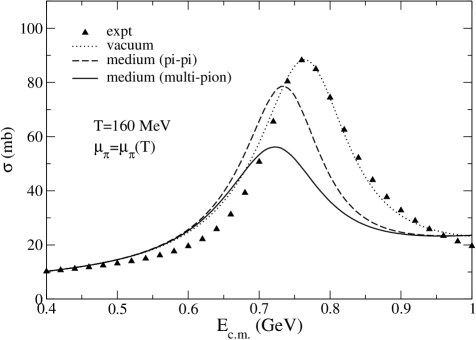
Figure 1: The $\pi\pi$ cross-section as a function of centre of mass energy. The dotted line indicates the cross-section obtained using eq. (29) which agrees well with the experimental values (eq. (26)) shown by filled triangles. The dashed and solid lines depict the in-medium cross-section for $\pi\pi$ and $\pi h~{}(=\pi,\omega,h_{1},a_{1})$ loops respectively in the $\rho$ and $\sigma$ self-energies evaluated at $T$=160 MeV with temperature dependent pion chemical potential.

The strong interaction dynamics of the pions enters the collision integrals through the cross-section. In Fig. 1 we show the $\pi\pi$ cross-section as a function of the centre of mass energy of scattering. The different curves are explained below. The filled triangles referred to as experiment is a widely used resonance saturation parametrization Bertsch1 ; Welke of isoscalar and isovector phase shifts obtained from various empirical data involving the $\pi\pi$ system. The isospin averaged differential cross-section is given by

$$\frac{d\sigma(s)}{d\Omega}=\frac{4}{q_{cm}^{2}}\left[\frac{1}{9}\sin^{2}\delta^{0}_{0}+\frac{5}{9}\sin^{2}\delta^{2}_{0}+\frac{1}{3}\cdot 9\sin^{2}\delta_{1}^{1}\cos^{2}\theta\right]$$ (26)

where

$$\delta^{0}_{0} = \frac{\pi}{2}+\arctan\left(\frac{E-m_{\sigma}}{\Gamma_{\sigma}/2}\right)$$

$$\delta_{1}^{1} = \frac{\pi}{2}+\arctan\left(\frac{E-m_{\rho}}{\Gamma_{\rho}/2}\right)$$

$$\delta^{2}_{0} = -0.12p/m_{\pi}~{}.$$ (27)

The widths are given by $\Gamma_{\sigma}=2.06p$ and $\Gamma_{\rho}=0.095p\left(\frac{p/m_{\pi}}{1+(p/m_{\rho})^{2}}\right)^{2}$ with $m_{\sigma}=5.8m_{\pi}$ and $m_{\rho}=5.53m_{\pi}$ . As seen in Fig. 2 these phase shifts agree quite well with those obtained from solutions of the Roy equations as given in Anantha . The bands bordered by the dotted lines represent the uncertainties in the solution. The experimentally measured phase shifts (not shown) have error bars Anantha which are not reflected in the parametrizations (27) plotted in Fig. 1.

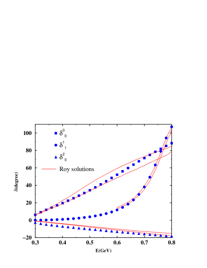
Figure 2: (Color online) The $\pi\pi$ phaseshifts (27) as a function of $E$ compared to Roy equation solutions given in Ref. Anantha

Our objective now is to set up a dynamical model which agrees reasonably with the above parametrization in vacuum and is amenable to the incorporation of medium effects using many body techniques. We thus evaluate the $\pi\pi$ cross-section involving $\rho$ and $\sigma$ meson exchange processes using the interaction Lagrangian

$${\cal L}=g_{\rho}\vec{\rho}^{\mu}\cdot\vec{\pi}\times\partial_{\mu}\vec{\pi}+\frac{1}{2}g_{\sigma}m_{\sigma}\vec{\pi}\cdot\vec{\pi}\sigma$$ (28)

where $g_{\rho}=6.05$ and $g_{\sigma}=2.5$. In the matrix elements corresponding to $s$-channel $\rho$ and $\sigma$ exchange diagrams which appear for total isospin $I=1$ and 0 respectively, we introduce a decay width in the corresponding propagator. We get Sukanya ,

$${\cal M}_{I=0} = g_{\sigma}^{2}m_{\sigma}^{2}\left[\frac{3}{s-m_{\sigma}^{2}+im_{\sigma}\Gamma_{\sigma}}+\frac{1}{t-m_{\sigma}^{2}}+\frac{1}{u-m_{\sigma}^{2}}\right]+2g_{\rho}^{2}\left[\frac{s-u}{t-m_{\rho}^{2}}+\frac{s-t}{u-m_{\rho}^{2}}\right]$$

$${\cal M}_{I=1} = g_{\sigma}^{2}m_{\sigma}^{2}\left[\frac{1}{t-m_{\sigma}^{2}}-\frac{1}{u-m_{\sigma}^{2}}\right]+g_{\rho}^{2}\left[\frac{2(t-u)}{s-m_{\rho}^{2}+im_{\rho}\Gamma_{\rho}}+\frac{t-s}{u-m_{\rho}^{2}}-\frac{u-s}{t-m_{\rho}^{2}}\right]$$

$${\cal M}_{I=2} = g_{\sigma}^{2}m_{\sigma}^{2}\left[\frac{1}{t-m_{\sigma}^{2}}+\frac{1}{u-m_{\sigma}^{2}}\right]+g_{\rho}^{2}\left[\frac{u-s}{t-m_{\rho}^{2}}+\frac{t-s}{u-m_{\rho}^{2}}\right]~{}.$$ (29)

The differential cross-section is then obtained from $\frac{d\sigma}{d\Omega}=\overline{|{\cal M}|^{2}}/64\pi^{2}s$ where the isospin averaged amplitude is given by $\overline{|{\cal M}|^{2}}=\frac{1}{9}\sum(2I+1)\overline{|{\cal M}_{I}|^{2}}$.

Considering the isoscalar and isovector contributions which involves $s$-channel $\sigma$ and $\rho$ meson exchange respectively, the integrated cross-section, shown by the dotted line (indicated by ’vacuum’) in Fig. 1 is seen to agree reasonably well with the experimental cross-section up to a centre of mass energy of about 1 GeV beyond which the theoretical estimate gives higher values. We hence use the experimental cross-section beyond this energy. Inclusion of the non-resonant $I=2$ contribution results in an overestimation and is ignored in this normalization of the model to experimental data. It is essential at this point to emphasize that the present approach of introducing finite decay widths for the exchanged resonances explicitly is not consistent with the well-known chiral low energy theorems concerning the amplitude for $\pi\pi$ scattering Weinberg_PRL as well as the scattering lengths.

We now construct the in-medium cross-section by introducing the effective propagator for the $\rho$ and $\sigma$ mesons in the above expressions for the matrix elements. We first discuss the case of the $\rho$ followed by the relatively simpler case of the $\sigma$ meson.

The in-medium propagator of the $\rho$ is obtained in terms of the self-energy by solving the Dyson equation and is given by

$$D_{\mu\nu}=D^{(0)}_{\mu\nu}+D^{(0)}_{\mu\sigma}\Pi^{\sigma\lambda}D_{\lambda\nu}$$ (30)

where $D^{(0)}_{\mu\nu}$ is the vacuum propagator for the $\rho$ meson and $\Pi^{\sigma\lambda}$ is the self energy function obtained from one-loop diagrams shown in Fig. 3. The standard procedure Bellac to solve this equation in the medium is to decompose the self-energy into transverse and longitudinal components. For the case at hand the difference between these components is found to be small and is hence ignored. We work with the polarization averaged self-energy function defined as

$$\Pi=\frac{1}{3}(2\Pi^{T}+q^{2}\Pi^{L})$$ (31)

where

$$\Pi^{T}=-\frac{1}{2}(\Pi_{\mu}^{\mu}+\frac{q^{2}}{\bar{q}^{2}}\Pi_{00}),~{}~{}~{}~{}\Pi^{L}=\frac{1}{\bar{q}^{2}}\Pi_{00},~{}~{}~{}\Pi_{00}\equiv u^{\mu}u^{\nu}\Pi_{{\mu\nu}}~{}.$$ (32)

The in-medium propagator is then written as

$$D_{\mu\nu}(q_{0},\vec{q})=\frac{-g_{\mu\nu}+q_{\mu}q_{\nu}/q^{2}}{q^{2}-m_{\rho}^{2}-{\rm Re}\Pi(q_{0},\vec{q})+i{\rm Im}\Pi(q_{0},\vec{q})}~{}.$$ (33)

The scattering, decay and regeneration processes which cause a gain or loss of $\rho$ mesons in the medium are responsible for the imaginary part of its self-energy. The real part on the other hand modifies the position of the pole of the spectral function.

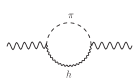
Figure 3: Self-energy diagrams where $h$ stands for $\pi,\omega,h_{1},a_{1}$ mesons.

In the real-time formulation of thermal field theory the self-energy assumes a 2$\times$2 matrix structure of which the 11-component is given by

$$\Pi_{{\mu\nu}}^{11}(q)=i\int\frac{d^{4}k}{(2\pi)^{4}}N_{{\mu\nu}}(q,k)D_{\pi}^{11}(k)D_{h}^{11}(q-k)$$ (34)

where $D^{11}$ is the 11-component of the scalar propagator given by $D^{11}(k)=\Delta(k)+2\pi if^{(0)}(k)\delta(k^{2}-m^{2})$. It turns out that the real and imaginary parts of the self-energy function which appear in eq. (33) can be obtained in terms of the 11-component through the relations Bellac ; Mallik_RT

$${\rm Re}\,\Pi_{{\mu\nu}} = {\rm Re}\,\Pi_{{\mu\nu}}^{11}$$

$${\rm Im}\Pi_{{\mu\nu}} = \epsilon(q_{0})\tanh(\beta q_{0}/2){\rm Im}\,\Pi_{{\mu\nu}}^{11}~{}.$$ (35)

Tensor structures associated with the two vertices and the vector propagator are included in $N_{{\mu\nu}}$ and are available in Ghosh1 where the interactions were taken from chiral perturbation theory. It is easy to perform the integral over $k_{0}$ using suitable contours to obtain

$${\Pi}^{{\mu\nu}}(q_{0},\vec{q}) = \int\frac{d^{3}k}{(2\pi)^{3}}\frac{1}{4\omega_{\pi}\omega_{h}}\left[\frac{(1+f^{(0)}(\omega_{\pi}))N^{{\mu\nu}}_{1}+f^{(0)}(\omega_{h})N^{{\mu\nu}}_{3}}{q_{0}-\omega_{\pi}-\omega_{h}+i\eta\epsilon(q_{0})}+\frac{-f^{(0)}(\omega_{\pi})N^{{\mu\nu}}_{1}+f^{(0)}(\omega_{h})N^{{\mu\nu}}_{4}}{q_{0}-\omega_{\pi}+\omega_{h}+i\eta\epsilon(q_{0})}\right.$$ (36)

$$+\left.\frac{f^{(0)}(\omega_{\pi})N^{{\mu\nu}}_{2}-f^{(0)}(\omega_{h})N^{{\mu\nu}}_{3}}{q_{0}+\omega_{\pi}-\omega_{h}+i\eta\epsilon(q_{0})}+\frac{-f^{(0)}(\omega_{\pi})N^{{\mu\nu}}_{2}-(1+f^{(0)}(\omega_{h}))N^{{\mu\nu}}_{4}}{q_{0}+\omega_{\pi}+\omega_{h}+i\eta\epsilon(q_{0})}\right]$$

where $f^{(0)}(\omega)=\frac{1}{e^{(\omega-\mu_{\pi})/T}-1}$ is the Bose distribution function with arguments $\omega_{\pi}=\sqrt{\vec{k}^{2}+m_{\pi}^{2}}$ and $\omega_{h}=\sqrt{(\vec{q}-\vec{k})^{2}+m_{h}^{2}}$. Note that this expression is a generalized form for the in-medium self-energy obtained by Weldon Weldon . The subscript $i(=1,..4)$ on $N^{{\mu\nu}}$ in (36) correspond to its values for $k_{0}=\omega_{\pi},-\omega_{\pi},q_{0}-\omega_{h},q_{0}+\omega_{h}$ respectively. It is easy to read off the real and imaginary parts from (36). The angular integration can be carried out using the $\delta$-functions in each of the four terms in the imaginary part which define the kinematically allowed regions in $q_{0}$ and $\vec{q}$ where scattering, decay and regeneration processes occur in the medium leading to the loss or gain of $\rho$ mesons Ghosh1 . The vector mesons $\omega$, $h_{1}$ and $a_{1}$ which appear in the loop have negative $G$-parity and have substantial $3\pi$ and $\rho\pi$ decay widths PDG . The (polarization averaged) self-energies containing these unstable particles in the loop graphs have thus been folded with their spectral functions,

$$\Pi(q,m_{h})=\frac{1}{N_{h}}\int^{(m_{h}+2\Gamma_{h})^{2}}_{(m_{h}-2\Gamma_{h})^{2}}dM^{2}\frac{1}{\pi}{\rm Im}\left[\frac{1}{M^{2}-m_{h}^{2}+iM\Gamma_{h}(M)}\right]\Pi(q,M)$$ (37)

with $N_{h}=\displaystyle\int^{(m_{h}+2\Gamma_{h})^{2}}_{(m_{h}-2\Gamma_{h})^{2}}dM^{2}\frac{1}{\pi}{\rm Im}\left[\frac{1}{M^{2}-m_{h}^{2}+iM\Gamma_{h}(M)}\right]$. The contributions from the loops with heavy mesons (the $\pi h$ loops) may then be considered as a multi-pion contribution to the $\rho$ self-energy.

The medium effect on propagation of the $\sigma$ meson is estimated analogously as above. The effective propagator in this case is given by

$$D(q_{0},\vec{q})=\frac{-1}{q^{2}-m_{\sigma}^{2}-{\rm Re}\Pi(q_{0},\vec{q})+i{\rm Im}\Pi(q_{0},\vec{q})}~{}.$$ (38)

Following the steps outlined above the expression for the self-energy of the $\sigma$ is given by

$${\Pi}(q_{0},\vec{q}) = N\int\frac{d^{3}k}{(2\pi)^{3}}\frac{1}{4\omega_{\pi}\omega_{\pi}^{\prime}}\left[\frac{1+f^{(0)}(\omega_{\pi})+f^{(0)}(\omega_{\pi}^{\prime})}{q_{0}-\omega_{\pi}-\omega_{\pi}^{\prime}+i\eta\epsilon(q_{0})}+\frac{f^{(0)}(\omega_{\pi}^{\prime})-f^{(0)}(\omega_{\pi})}{q_{0}-\omega_{\pi}+\omega_{\pi}^{\prime}+i\eta\epsilon(q_{0})}\right.$$ (39)

$$+\left.\frac{f^{(0)}(\omega_{\pi})-f^{(0)}(\omega_{\pi}^{\prime})}{q_{0}+\omega_{\pi}-\omega_{\pi}^{\prime}+i\eta\epsilon(q_{0})}-\frac{1+f^{(0)}(\omega_{\pi})+f^{(0)}(\omega_{\pi}^{\prime})}{q_{0}+\omega_{\pi}+\omega_{\pi}^{\prime}+i\eta\epsilon(q_{0})}\right]$$

where $\omega_{\pi}^{\prime}=\sqrt{(\vec{q}-\vec{k})^{2}+m_{\pi}^{2}}$. The imaginary part for the kinematic region of our interest in this case receives contribution only from the first term which essentially describes the decay of the $\sigma$ into two pions minus the reverse process of formation.

The in-medium cross-section is now obtained by using the full $\rho$ and $\sigma$ propagators given by (33) and (38) respectively in place of the vacuum propagators in the scattering amplitudes. The long dashed line in Fig. 1 shows a suppression of the peak when only the $\pi\pi$ loop in the $\rho$ and $\sigma$ self-energies are considered. This effect is magnified when the $\pi h$ loops containing heavier mesons in the $\rho$ self-energy are taken into account and is depicted by the solid line indicated by multi-pion. This is also accompanied by a small shift in the peak position. Extension to the case of finite baryon density can be done using the spectral function computed in Ghosh2 where an extensive list of baryon (and anti-baryon) loops are considered along with the mesons. A similar modification of the $\pi\pi$ cross-section for a hot and dense system was seen also in Bertsch2 .

Figure 4: The pion chemical potential as a function of temperature Hirano .

We end this section with a discussion of the pion chemical potential. As mentioned in the introduction, in heavy ion collisions pions get out of chemical equilibrium early at $T\sim$ 170 MeV and a corresponding chemical potential starts building up with decrease in temperature. The kinetics of the gas is then dominated by elastic collisions including resonance formation such as $\pi\pi\leftrightarrow\rho$ etc. At still lower temperature, $T\sim$ 100 MeV elastic collisions become rarer and the momentum distribution gets frozen resulting in kinetic freeze-out. This scenario is quite compatible with the treatment of medium modification of the $\pi\pi$ cross-section being employed in this work where the $\pi\pi$ interaction is mediated by $\rho$ and $\sigma$ exchange and the subsequent propagation of these mesons are modified by two-pion and effective multi-pion fluctuations. We take the temperature dependent pion chemical potential from Ref. Hirano which implements the formalism described in Bebie and reproduces the slope of the transverse momentum spectra of identified hadrons observed in experiments. Here, by fixing the ratio $s/n$ where $s$ is the entropy density and $n$ the number density to the value at chemical freeze-out where $\mu_{\pi}=0$, one can go down in temperature up to the kinetic freeze-out by increasing the pion chemical potential. This provides the temperature dependence leading to $\mu_{\pi}(T)$ which is shown in Fig. 4. In this partial chemical equilibrium scenario of Bebie the chemical potentials of the heavy mesons are determined from elementary processes. The $\omega$ chemical potential e.g. is given by $\mu_{\omega}=3\times 0.88\mu_{\pi}$, as a consequence of the processes $\omega\leftrightarrow\pi\pi\pi$ occurring in the medium. The branching ratios are taken from PDG .

IV Results

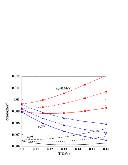
Figure 5: (Color online)The bulk viscosity in various scenarios as a function of $T$. The upper (with circles), middle (with triangles) and lower sets of curves correspond to $\mu_{\pi}=85$ MeV, $\mu_{\pi}=\mu_{\pi}(T)$ and $\mu_{\pi}=0$ respectively. In each set the solid line represents use of vacuum cross-section, the dotted line for in-medium modification due to pion loop and the dashed line for loops with heavy particles in addition.

We begin with the results for bulk viscosity $\zeta$ as a function of temperature $T$. In Fig. 5 the three sets of curves correspond to different values of the pion chemical potential. The uppermost set of curves (with circles) show the bulk viscosity calculated with a pion chemical potential $\mu_{\pi}\sim 85$ MeV. The corresponding curves in the lowermost set are evaluated with $\mu_{\pi}=0$. These values are representative of the kinetic and chemical freeze-out in heavy ion collisions respectively. The solid line in the lowermost set represents the case where the vacuum cross-section given by eq. (29) is used and agrees with the estimate in Davesne . The set of curves with triangles depicts the situation when $\mu_{\pi}$ is a (decreasing) function of temperature as shown in Fig. 4. This resembles the situation encountered in the later stages of heavy ion collisions and interpolates between the results with the constant values of the pion chemical potential discussed before. The three curves in each set show the effect of medium on the $\pi\pi$ cross-section. The short-dashed lines in each of the sets depict medium effects for pion loops in the $\rho$ propagator and the long dashed lines correspond to the situation when the heavy mesons are included i.e. for $\pi h$ loops where $h=\pi,\omega,h_{1},a_{1}$. The clear separation between the curves in each set displays a significant effect brought about by the medium dependence of the cross-section. A large dependence on the pion chemical potential is also inferred since the three sets of curves appear nicely separated.

Figure 6: The entropy density of an interacting pion gas as a function of $T$ for different values of the pion chemical potential.

Figure 7: $\zeta/s$ as a function of $T$ for different $\pi\pi$ cross-section. The temperature dependent pion chemical potential has been used in all cases.

Viscosities for relativistic fluids are generally expressed in terms of a dimensionless ratio obtained by dividing with the entropy density. The latter is obtained from the thermodynamic relation

$$Ts=\epsilon+P-n\mu_{\pi}~{}.$$ (40)

For a free pion gas, we get on using the relations for the energy density $\epsilon$, pressure $P$ and number density $n$ from Appendix-A,

$$s=\frac{g_{\pi}}{2\pi^{2}}\ m_{\pi}^{2}[m_{\pi}S_{3}^{1}(z)-\mu_{\pi}S_{2}^{1}(z)]~{}.$$ (41)

Here $g_{\pi}=3$, $z=m_{\pi}/T$ and the functions $S_{n}^{\alpha}(z)$ are given in Appendix-A . Interactions between pions lead to corrections to this formula. To $O(T^{6})$ this has been calculated for finite pion chemical potential in Nicola using chiral perturbation theory to give

$$\Delta s=-\frac{3m_{\pi}^{4}}{16\pi^{4}f_{\pi}^{2}}S_{1}^{1}(z)[m_{\pi}S_{2}^{0}(z)-\mu_{\pi}S_{1}^{0}(z)]$$ (42)

where $f_{\pi}=93$ MeV. It is easily verified that this expression reduces for $\mu_{\pi}=0$ to those given in Gerber ; Lang . This correction is $\sim 1-2\%$ for values of $\mu_{\pi}$ and $T$ considered here. In Fig. 6 the entropy density of an interacting pion gas as a function of temperature is shown for three values of the pion chemical potential as discussed in the context of Fig. 5.

In Fig. 7 we show $\zeta/s$ as a function of $T$ using the temperature dependent pion chemical potential. The medium dependence is clearly observed when we compare the results obtained with the vacuum cross-section with the ones where the $\sigma$ and $\rho$ propagation is modified due to $\pi\pi$ and $\pi h$ (multi-pion) loops. The decreasing trend with increasing temperature was observed also in Moore and Dobado_bulk .

Figure 8: $\eta$ as a function of $T$ for different values of the $\pi\pi$ cross-section. The temperature dependent pion chemical potential has been used in all cases.

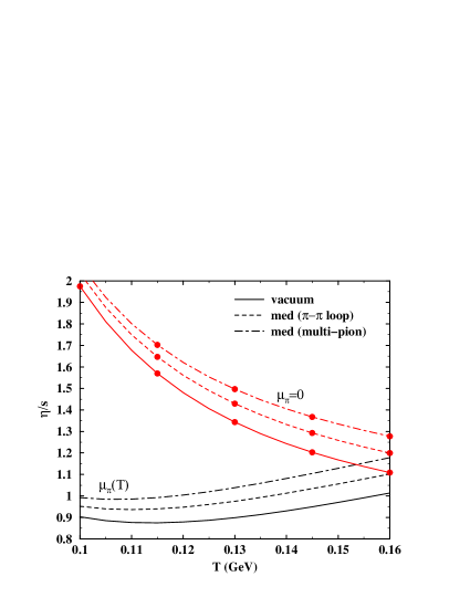
Figure 9: (Color online)$\eta/s$ as a function of $T$. The upper set of curves with circles correspond to $\mu_{\pi}=0$ and the lower set corresponds to $\mu_{\pi}=\mu_{\pi}(T)$.

We now turn to the shear viscosity. Here we extend the work in Ref. Sukanya to include the effect of the pion chemical potential. Shown in Fig. 8 is the shear viscosity as a function of $T$ where the results with $\pi\pi$ and $\pi h$ loops are contrasted with the case where the vacuum cross-section is used. The result with the vacuum cross-section agrees with Dobado3 and Davesne for $\mu_{\pi}=0$. A noticeable medium effect is observed as indicated by the short and long-dashed lines.

Finally, in Fig. 9 we show results for $\eta/s$. For $\mu_{\pi}=0$ the upper set of curves with filled circles show the usual decreasing trend as seen, for example in Nakano . This trend is reversed when $\mu_{\pi}(T)$ is used and $\eta/s$ increases with $T$ in contrast to $\zeta/s$ which decreases. The values in all cases remain well above $1/4\pi$.

V Summary and Outlook

In this work we have evaluated the viscosities of a pion gas by solving the Uehling-Uhlenbeck transport equation in the Chapman-Enskog approximation to leading order with an aim to study the effect of a medium dependent cross-section. The $\pi\pi$ cross-section which goes as an input to these calculations is evaluated from $\sigma$ and $\rho$ exchange processes. Spectral modifications of the $\rho$ and $\sigma$ propagators implemented through $\pi h$ and $\pi\pi$ self-energy diagrams respectively show a significant effect on the cross-section and consequently on the temperature dependence of transport coefficients. The effect of early chemical freeze-out in heavy ion collisions is implemented through a temperature dependent pion chemical potential which also enhances the medium effect. Results for $\zeta/s$ and $\eta/s$ also show a significant medium dependence in this scenario.

The viscous coefficients and their temperature dependence could affect the quantitative estimates of signals of heavy ion collisions particularly where hydrodynamic simulations are involved. For example, it has been argued in Dusling that corrections to the freeze-out distribution due to bulk viscosity can be significant. As a result the hydrodynamic description of the $p_{T}$ spectra and elliptic flow of hadrons could be improved by including a realistic temperature dependence of the viscous coefficients. Studies in this direction are in progress.

VI Appendix A

The integrals over Bose functions which appear in the definitions of thermodynamic quantities like energy density, pressure, entropy etc. of a pion gas can be expressed in terms of the functions $S_{n}^{\alpha}(z)$ where $z=m/T$. Some of these which appear in various expressions in this work are given by

$$S_{1}^{1}(z) = \frac{2\pi^{2}}{zT^{2}}\int\ d\Gamma_{p}f^{(0)}(p)$$

$$S_{2}^{1}(z) = \frac{2\pi^{2}}{z^{2}T^{3}}\int\ d\Gamma_{p}\ E\ f^{(0)}(p)$$

$$S_{3}^{2}(z) = \frac{2\pi^{2}}{3z^{3}T^{5}}\int\ d\Gamma_{p}\ p^{2}E\ f^{(0)}(p)$$ (A.1)

where $E=\sqrt{p^{2}+m^{2}}$, $f^{(0)}(p)=[e^{\beta(E-\mu)}-1]^{-1}$ and $d\Gamma_{p}=d^{3}p/(2\pi)^{3}E$. Using the formula $[a-1]^{-1}=\displaystyle\sum_{n=1}^{\infty}(a^{-1})^{n}$ these integrals can be converted to sums over infinite series and can be compactly expressed as $S_{n}^{\alpha}(z)=\displaystyle\sum_{k=1}^{\infty}e^{k\mu/T}k^{-\alpha}K_{n}(kz)$, $K_{n}(x)$ denoting the modified Bessel function of order $n$ given by

$$K_{n}(x)=\frac{2^{n}n!}{(2n)!\ x^{n}}\int_{x}^{\infty}\ d\tau(\tau^{2}-x^{2})^{n-\frac{1}{2}}e^{-\tau}$$ (A.2)

or

$$K_{n}(x)=\frac{2^{n}n!(2n-1)}{(2n)!\ x^{n}}\int_{x}^{\infty}\ \tau d\tau(\tau^{2}-x^{2})^{n-\frac{3}{2}}e^{-\tau}~{}.$$ (A.3)

Using now the property

$$\frac{\partial}{\partial(\mu/T)}S_{n}^{\alpha}(z)=S_{n}^{\alpha-1}(z)$$ (A.4)

the remaining integrals may be easily obtained. The equilibrium formulae for the number density, pressure, energy density and enthalpy density are respectively given by

$$n = g\int d\Gamma_{p}E_{p}f^{(0)}(p)=\frac{g}{2\pi^{2}}z^{2}T^{3}S_{2}^{1}(z),$$

$$P = g\int d\Gamma_{p}\frac{\vec{p}^{2}}{3}f^{(0)}(p)=\frac{g}{2\pi^{2}}z^{2}T^{4}S_{2}^{2}(z),$$

$$\epsilon=ne = g\int d\Gamma_{p}E_{p}^{2}f^{(0)}(p)=\frac{g}{2\pi^{2}}z^{2}T^{4}[zS_{3}^{1}(z)-S_{2}^{2}(z)]$$

$$H = nh=nzT\frac{S_{3}^{1}(z)}{S_{2}^{1}(z)}~{},$$ (A.5)

where for a pion gas $g=3$. In these appendices we have suppressed the subscript ’$\pi$’ on $m$ and $\mu$ for brevity.

VII Appendix B

Here we show how the left side of the linearized transport equation (5) given by

$$p^{\mu}\partial_{\mu}f^{(0)}(x,p)=-{\cal L}[\phi]$$ (B.1)

can be expressed in terms of thermodynamic forces. We write $\partial_{\mu}=u_{\mu}u^{\nu}\partial_{\nu}+\Delta_{\mu\nu}\partial^{\nu}\equiv u_{\mu}D+\nabla_{\mu}$ separating the time derivative $D$ and the gradient $\nabla_{\mu}$. Note that $D\to\partial/\partial t$ and $\nabla_{\mu}\to\partial_{i}$ in the local rest frame. On differentiating $f^{(0)}$

$$(p\cdot u)\left[\frac{p\cdot u}{T^{2}}DT+D(\frac{\mu}{T})-\frac{p^{\mu}}{T}Du_{\mu}\right]+p^{\mu}\left[\frac{p\cdot u}{T^{2}}\nabla_{\mu}T+\nabla_{\mu}(\frac{\mu}{T})-\frac{p^{\nu}}{T}\nabla_{\mu}u_{\nu}\right]=-\frac{{\cal L}[\phi]}{f^{(0)}(1+f^{(0)})}~{}.$$ (B.2)

The terms $DT$ and $D(\frac{\mu}{T})$ do not appear in the expression of the thermodynamic forces and are to be eliminated using equilibrium laws. From the equation of continuity

$$\partial_{\mu}N^{\mu}=0$$

where $N^{\mu}=nu^{\mu}$, we get

$$Dn=-n\partial_{\mu}u^{\mu}~{}.$$ (B.3)

Again, contracting the equation for energy-momentum conservation with $u_{\mu}$ i.e.

$$u_{\mu}\partial_{\nu}T^{{\mu\nu}\,(0)}=0$$

where $T^{{\mu\nu}\,(0)}=n[(e+\frac{P}{n})u^{\mu}u^{\nu}-g^{\mu\nu}\frac{P}{n}]$ results in the relation

$$De=-\frac{P}{n}\partial_{\mu}u^{\mu}~{}.$$ (B.4)

Further, contracting with the projector $\Delta^{\mu\nu}$,

$$\Delta^{\mu}_{\nu}\partial_{\alpha}T^{\nu\alpha\,(0)}=0$$

yields

$$Du^{\mu}=\frac{1}{nh}\nabla^{\mu}P~{}.$$ (B.5)

Making use of the relativistic Gibbs-Duhem relation

$$\partial^{\mu}P=nT\partial^{\mu}(\frac{\mu}{T})+nhT^{-1}\partial^{\mu}T$$

and (B.4) in (B.5) we get

$$Dh=TD(\frac{\mu}{T})+hT^{-1}DT~{}.$$ (B.6)

Using now the expansions

$$De = \left.\frac{\partial e}{\partial T}\right|_{\mu/T}DT+\left.\frac{\partial e}{\partial(\mu/T)}\right|_{T}D(\frac{\mu}{T})$$

$$Dh = \left.\frac{\partial h}{\partial T}\right|_{\mu/T}DT+\left.\frac{\partial h}{\partial(\mu/T)}\right|_{T}D(\frac{\mu}{T})$$ (B.7)

on the left hand sides of eqs. (B.4) and (B.6) results in a coupled set of equations for $DT$ and $D(\mu/T)$. These are easily solved to arrive at

$$DT = \frac{(P/n)\left[T-\left.\frac{\partial h}{\partial(\mu/T)}\right|_{T}\right]\partial_{\mu}u^{\mu}}{\left.\frac{\partial e}{\partial(\mu/T)}\right|_{T}\left[hT^{-1}-\left.\frac{\partial h}{\partial T}\right|_{\mu/T}\right]-\left.\frac{\partial e}{\partial T}\right|_{\mu/T}\left[T-\left.\frac{\partial h}{\partial(\mu/T)}\right|_{T}\right]}$$

$$D(\frac{\mu}{T}) = \frac{-(P/n)\left[hT^{-1}-\left.\frac{\partial h}{\partial T}\right|_{\mu/T}\right]\partial_{\mu}u^{\mu}}{\left.\frac{\partial e}{\partial(\mu/T)}\right|_{T}\left[hT^{-1}-\left.\frac{\partial h}{\partial T}\right|_{\mu/T}\right]-\left.\frac{\partial e}{\partial T}\right|_{\mu/T}\left[T-\left.\frac{\partial h}{\partial(\mu/T)}\right|_{T}\right]}~{}.$$ (B.8)

We next evaluate the partial derivatives of $e$ and $h$ with respect $T$ and $(\mu/T)$ using the relations in Appendix-A. We get

$$\left.\frac{\partial h}{\partial T}\right|_{\mu/T} = z\left[5\frac{S_{3}^{1}}{S_{2}^{1}}+z\frac{S_{2}^{0}}{S_{2}^{1}}-z\frac{S_{3}^{1}S_{3}^{0}}{(S_{2}^{1})^{2}}\right]$$

$$\left.\frac{\partial e}{\partial T}\right|_{\mu/T} = 4z\frac{S_{3}^{1}}{S_{2}^{1}}+z\frac{S_{2}^{2}S_{3}^{0}}{(S_{2}^{1})^{2}}-\frac{S_{2}^{2}}{S_{2}^{1}}+z^{2}\left[\frac{S_{2}^{0}}{S_{2}^{1}}-\frac{S_{3}^{1}S_{3}^{0}}{(S_{2}^{1})^{2}}\right]$$

$$\left.\frac{\partial h}{\partial(\mu/T)}\right|_{T} = Tz\left[\frac{S_{3}^{0}}{S_{2}^{1}}-\frac{S_{3}^{1}S_{2}^{0}}{(S_{2}^{1})^{2}}\right]$$

$$\left.\frac{\partial e}{\partial(\mu/T)}\right|_{T} = -T\left[1-\frac{S_{2}^{2}S_{2}^{0}}{(S_{2}^{1})^{2}}\right]+Tz\left[\frac{S_{3}^{0}}{S_{2}^{1}}-\frac{S_{3}^{1}S_{2}^{0}}{(S_{2}^{1})^{2}}\right]~{}.$$ (B.9)

Putting these in (B.8) we get

$$T^{-1}DT = (1-\gamma^{\prime})\partial_{\mu}u^{\mu}$$

$$TD(\frac{\mu}{T}) = \left[(\gamma^{\prime\prime}-1)h-\gamma^{\prime\prime\prime}T\right]\partial_{\mu}u^{\mu}$$ (B.10)

where

$$\gamma^{\prime}=\frac{(S_{2}^{0}/S_{2}^{1})^{2}-(S_{3}^{0}/S_{2}^{1})^{2}+4z^{-1}S_{2}^{0}S_{3}^{1}/(S_{2}^{1})^{2}+z^{-1}S_{3}^{0}/S_{2}^{1}}{(S_{2}^{0}/S_{2}^{1})^{2}-(S_{3}^{0}/S_{2}^{1})^{2}+3z^{-1}S_{2}^{0}S_{3}^{1}/(S_{2}^{1})^{2}+2z^{-1}S_{3}^{0}/S_{2}^{1}-z^{-2}}$$ (B.11)

$$\gamma^{\prime\prime}=1+\frac{z^{-2}}{(S_{2}^{0}/S_{2}^{1})^{2}-(S_{3}^{0}/S_{2}^{1})^{2}+3z^{-1}S_{2}^{0}S_{3}^{1}/(S_{2}^{1})^{2}+2z^{-1}S_{3}^{0}/S_{2}^{1}-z^{-2}}$$ (B.12)

$$\gamma^{\prime\prime\prime}=\frac{S_{2}^{0}/S_{2}^{1}+5z^{-1}S_{3}^{1}/S_{2}^{1}-S_{3}^{0}S_{3}^{1}/(S_{2}^{1})^{2}}{(S_{2}^{0}/S_{2}^{1})^{2}-(S_{3}^{0}/S_{2}^{1})^{2}+3z^{-1}S_{2}^{0}S_{3}^{1}/(S_{2}^{1})^{2}+2z^{-1}S_{3}^{0}/S_{2}^{1}-z^{-2}}$$ (B.13)

We now come back to eq. (B.2) in which we replace $DT$, $D(\frac{\mu}{T})$ and $Du^{\mu}$ using eqs. (B.8) and (B.5) to get

$$(p\cdot u)p_{\mu}\left[\frac{\nabla^{\mu}T}{T}-\frac{\nabla^{\mu}P}{nh}\right]+Tp_{\mu}\nabla^{\mu}(\frac{\mu}{T})-p_{\mu}p_{\nu}\left[\nabla^{\mu}u^{\nu}-\frac{1}{3}\Delta^{\mu\nu}\nabla\cdot u\right]+$$

$$\left[(p.u)^{2}(1-\gamma^{\prime})+p\cdot u\left\{(\gamma^{\prime\prime}-1)h-\gamma^{\prime\prime\prime}T\right\}-\frac{1}{3}p_{\mu}p_{\nu}\Delta^{\mu\nu}\right]\partial\cdot u=-\frac{T{\cal L}[\phi]}{f^{(0)}(1+f^{(0)})}$$ (B.14)

which on further simplification and rearrangement gives

$$[Q\partial\cdot u+p_{\mu}\Delta^{\mu\nu}(p\cdot u-h)(T^{-1}\partial_{\nu}T-Du_{\nu})-\langle p_{\mu}p_{\nu}\rangle\langle\partial^{\mu}u^{\nu}\rangle]f^{(0)}(1+f^{(0)})=-T{\cal L}[\phi]$$ (B.15)

where the abbreviation

$$Q=-\frac{1}{3}m^{2}+(p\cdot u)^{2}\{\frac{4}{3}-\gamma{{}^{\prime}}\}+p\cdot u\{(\gamma{{}^{\prime\prime}}-1)h-\gamma{{}^{\prime\prime\prime}}T\}~{}.$$ (B.16)

and

$$\langle\partial^{\mu}u^{\nu}\rangle = \left[\nabla^{\mu}u^{\nu}-\frac{1}{3}\Delta^{\mu\nu}\nabla\cdot u\right]$$

$$\langle p_{\mu}p_{\nu}\rangle = p_{\mu}p_{\nu}-\frac{p^{2}}{3}\Delta_{\mu\nu}-p\cdot u(p_{\mu}u_{\nu}+p_{\nu}u_{\mu}-\frac{1}{3}g_{\mu\nu}p\cdot u)+\frac{2}{3}(p\cdot u)^{2}u_{\mu}u_{\nu}~{}.$$ (B.17)

VIII Appendix C

Here we briefly describe how the leading order expressions for the viscosities are obtained from the integral equations (13) and (14). Let us first consider the bulk viscosity $\zeta$. Following Polak ; Davesne we multiply both sides of eq. (13) by Laguerre polynomial of order 1/2 and degree $n$ and integrate over $d\Gamma_{p}$ to get

$$[A(\tau),L_{n}^{{1}/{2}}(\tau)]=\frac{\alpha_{n}}{n}$$ (C.1)

where $\tau=\beta(p\cdot u-m)$ and

$$\alpha_{n}=-\frac{1}{nT}\int d\Gamma_{p}f^{(0)}(p)\{1+f^{(0)}(p)\}QL_{n}^{{1}/{2}}(\tau)~{}.$$ (C.2)

and the abreviation

$$[F,G]=\frac{1}{4n^{2}}\int d\Gamma_{p}d\Gamma_{k}d\Gamma_{p^{\prime}}\ d\Gamma_{k^{\prime}}f^{(0)}(p)f^{(0)}(k)\{1+f^{(0)}(p^{\prime})\}\{1+f^{(0)}(k^{\prime})\}\delta(F)\delta(G)\ W$$ (C.3)

with

$$\delta(F) = F(p)+F(k)+F(p^{\prime})+F(k^{\prime})$$

$$\delta(G) = G(p)+G(k)+G(p^{\prime})+G(k^{\prime})~{}.$$ (C.4)

Expanding $A$ as

$$A(\tau)=\sum_{m=0}^{\infty}a_{m}L_{m}^{{1}/{2}}(\tau)$$ (C.5)

and putting in (C.1) the expression for bulk viscosity to first order is obtained as

$$\zeta=T\frac{\alpha_{2}^{2}}{a_{22}}$$ (C.6)

where $\alpha_{2}$ is given by eq. (C.2) with $n=2$. The denominator $a_{22}$ in (21) can be expressed using (C.3) as

$$a_{22}=[L_{2}^{{1}/{2}}(\tau),L_{2}^{{1}/{2}}(\tau)]$$ (C.7)

and involves a 12-dimensional integral. This is considerably simplified by making a change of variables as described in Davesne ; Polak reducing the number of integrations essentially to five so that

$$a_{22} = \frac{m^{6}}{2\pi^{4}n^{2}}\int_{0}^{\infty}d\chi\int_{0}^{\infty}d\psi\int_{0}^{\pi}d\theta\int_{0}^{2\pi}d\phi\int_{0}^{\pi}d\Theta$$ (C.8)

$$\times f^{(0)}(p)f^{(0)}(k)\{1+f^{(0)}(p^{\prime})\}\{1+f^{(0)}(k^{\prime})\}$$

$$\times \delta\{L_{2}^{{1}/{2}}(\tau)\}\delta\{L_{2}^{{1}/{2}}(\tau)\}\frac{1}{2}\frac{d\sigma}{d\Omega}(\psi,\Theta)$$

$$\times \sinh^{2}\chi\sinh^{3}\psi\cosh^{3}\psi\sin\Theta\sin\theta~{}.$$

Using now

$$f^{(0)}(p)f^{(0)}(k)\{1+f^{(0)}(p^{\prime})\}\{1+f^{(0)}(k^{\prime})\}=\frac{e^{-2\mu/T}e^{2z\cosh\psi\cosh\chi}}{(e^{E}-1)(e^{F}-1)(e^{G}-1)(e^{H}-1)}$$

where the exponents in the Bose functions are given by

$$E = z(\cosh\psi\cosh\chi-\sinh\psi\sinh\chi\cos\theta)-\mu/T$$

$$F = z(\cosh\psi\cosh\chi-\sinh\psi\sinh\chi\cos\theta^{\prime})-\mu/T$$

$$G = E+2z\sinh\psi\sinh\chi\cos\theta$$

$$H = F+2z\sinh\psi\sinh\chi\cos\theta^{\prime}$$ (C.9)

and

$$\delta\{L_{2}^{{1}/{2}}(\tau)\}\delta\{L_{2}^{{1}/{2}}(\tau)\}=z^{4}(\sinh\psi\sinh\chi)^{4}(\cos^{2}\theta-\cos^{2}\theta^{\prime})^{2}$$ (C.10)

we finally get

$$a_{22}=2z^{2}I_{3}(z)~{}.$$ (C.11)

The relative angle $\theta^{\prime}$ is defined by, $\cos\theta^{\prime}=\cos\theta\cos\Theta-\sin\theta\sin\Theta\cos\phi~{}.$ Also, on simplification, the integral $\alpha_{2}$ is finally given by

$$\alpha_{2} = \frac{z^{3}}{2}[\frac{1}{3}(\frac{S_{3}^{0}}{S_{2}^{1}}-z^{-1})+(\frac{S_{2}^{0}}{S_{2}^{1}}+\frac{3}{z}\frac{S_{3}^{1}}{S_{2}^{1}})\{(1-\gamma^{\prime\prime})\frac{S_{3}^{1}}{S_{2}^{1}}+\gamma^{\prime\prime\prime}z^{-1}\}$$ (C.12)

$$- (\frac{4}{3}-\gamma^{\prime})\{\frac{S_{3}^{0}}{S_{2}^{1}}+15z^{-2}\frac{S_{3}^{2}}{S_{2}^{1}}+2z^{-1}\}]~{}.$$

The calculation for the shear viscosity $\eta$ follows a similar procedure and is more involved because of the tensorial nature of $C_{\mu\nu}=C\langle p_{\mu}p_{\nu}\rangle$. In this case eq. (14) is multiplied by Laguerre polynomial of order $5/2$ on both sides and then integrated over $d\Gamma_{p}$ to get the formal expression

$$[C(\tau)\langle p_{\mu}p_{\nu}\rangle,L_{n}^{{5}/{2}}(\tau)\langle p^{\mu}p^{\nu}\rangle]=\frac{m}{n}T\gamma_{n}$$ (C.13)

where

$$\gamma_{n}=-\frac{1}{mnT^{2}}\int d\Gamma_{p}f^{(0)}(p)\{1+f^{(0)}(p)\}L_{n}^{{5}/{2}}(\tau)\langle p_{\mu}p_{\nu}\rangle\langle p^{\mu}p^{\nu}\rangle~{}.$$ (C.14)

Writing in this case

$$C(\tau)=\sum_{m=0}^{\infty}c_{m}L_{m}^{{5}/{2}}(\tau)$$ (C.15)

and putting in (C.13), the first approximation to $\eta$ is obtained as

$$\eta=\frac{T}{10}\ \frac{\gamma_{0}^{2}}{c_{00}}$$ (C.16)

where

$$c_{00}=\frac{1}{m^{2}T^{2}}[L_{0}^{{5}/{2}}(\tau)\langle p_{\mu}p_{\nu}\rangle,L_{0}^{{5}/{2}}(\tau)\langle p^{\mu}p^{\nu}\rangle]~{}.$$ (C.17)

Simplification along the lines of Davesne ; Polak finally yields

$$\gamma_{0} = -10\frac{S_{3}^{2}(z)}{S_{2}^{1}(z)}~{},$$

$$c_{00} = 16I_{1}(z)+16I_{2}(z)+\frac{16}{3}I_{3}(z)~{}.$$ (C.18)

The integrals $I_{\alpha}(z)$ are defined as

$$I_{\alpha}(z) = \frac{z^{4}}{[S_{2}^{1}(z)]^{2}}\ e^{(-2\mu/T)}\int_{0}^{\infty}d\psi\ \cosh^{3}\psi\sinh^{7}\psi\int_{0}^{\pi}d\Theta\sin\Theta\frac{1}{2}\frac{d\sigma}{d\Omega}(\psi,\Theta)\int_{0}^{2\pi}d\phi$$ (C.19)

$$\int_{0}^{\infty}d\chi\sinh^{2\alpha}\chi\int_{0}^{\pi}d\theta\sin\theta\frac{e^{2z\cosh\psi\cosh\chi}}{(e^{E}-1)(e^{F}-1)(e^{G}-1)(e^{H}-1)}\ M_{\alpha}(\theta,\Theta)$$

where the functions $M_{\alpha}$ stand for

$$M_{1}(\theta,\Theta) = 1-\cos^{2}\Theta~{},$$

$$M_{2}(\theta,\Theta) = \cos^{2}\theta+\cos^{2}\theta^{\prime}-2\cos\theta\cos\theta^{\prime}\cos\Theta~{},$$

$$M_{3}(\theta,\Theta) = [\cos^{2}\theta-\cos^{2}\theta^{\prime}]^{2}$$ (C.20)

References

- (1) P. Kovtun, D. T. Son and A. O. Starinets, Phys. Rev. Lett. 94, 111601 (2005).
- (2) L. P. Csernai, J. I. Kapusta and L. D. McLerran, Phys. Rev. Lett. 97, 152303 (2006).
- (3) A. Rebhan and D. Steineder, Phys. Rev. Lett. 108 (2012) 021601
- (4) M. Cheng et al., Phys. Rev. D 81 (2010) 054504
- (5) D. Kharzeev and K. Tuchin, JHEP 0809 (2008) 093
- (6) A. Dobado, F. J. Llanes-Estrada and J. M. Torres-Rincon, Phys. Rev. D 80 (2009) 114015
- (7) A. Dobado and J. M. Torres-Rincon, Phys. Rev. D 86 (2012) 074021
- (8) J. -W. Chen and J. Wang, Phys. Rev. C 79 (2009) 044913
- (9) D. N. Zubarev, Non-equilibrium Statistical Thermodynamics (Consultants Bureau, NN, 1974).
- (10) A. Hosoya, M. a. Sakagami and M. Takao, Annals Phys. 154 (1984) 229.
- (11) R. Lang, N. Kaiser and W. Weise, Eur. Phys. J. A 48 (2012) 109
- (12) S. Mallik and S. Sarkar, arXiv:1211.2588 [nucl-th].
- (13) S. Jeon and L. G. Yaffe, Phys. Rev. D 53, 5799 (1996).
- (14) S. Weinberg, Physica A 96 (1979) 327.
- (15) J. Gasser and H. Leutwyler, Annals Phys. 158, 142 (1984).
- (16) A. Dobado and S. N. Santalla, Phys. Rev. D 65, 096011 (2002).
- (17) J. W. Chen, Y. H. Li, Y. F. Liu and E. Nakano, Phys. Rev. D 76, 114011 (2007)
- (18) A. Dobado and F. J. Llanes-Estrada, Phys. Rev. D 69, 116004 (2004).
- (19) K. Itakura, O. Morimatsu and H. Otomo, Phys. Rev. D 77, 014014 (2008).
- (20) M. Prakash, M. Prakash, R. Venugopalan and G. Welke, Phys. Rept. 227 (1993) 321.
- (21) D. Davesne, Phys. Rev. C 53, 3069 (1996).
- (22) E. Lu and G. D. Moore, Phys. Rev. C 83 (2011) 044901
- (23) D. Fernandez-Fraile and A. Gomez Nicola, Phys. Rev. Lett. 102 (2009) 121601
- (24) G. Bertsch, M. Gong, L. D. McLerran, P. V. Ruuskanen and E. Sarkkinen, Phys. Rev. D 37 (1988) 1202.
- (25) A. Dobado and F. J. Llanes-Estrada, Eur. Phys. J. C 49 (2007) 1011
- (26) S. Mitra, S. Ghosh and S. Sarkar, Phys. Rev. C 85 (2012) 064917
- (27) P. Chakraborty and J. I. Kapusta, Phys. Rev. C 83 (2011) 014906.
- (28) W. A. Van Leeuwen, P. H. Polak and S. R. De Groot, Physica 66, 455 (1973).
- (29) G. M. Welke, R. Venugopalan and M. Prakash, Phys. Lett. B 245 (1990) 137.
- (30) B. Ananthanarayan, G. Colangelo, J. Gasser and H. Leutwyler, Phys. Rept. 353 (2001) 207
- (31) S. Weinberg, Phys. Rev. Lett. 17 (1966) 616.
- (32) M. Le Bellac, Thermal Field Theory (Cambridge University Press, Cambridge, 1996).
- (33) S. Mallik and S. Sarkar, Eur. Phys. J. C 61, 489 (2009).
- (34) S. Ghosh, S. Sarkar and S. Mallik, Eur. Phys. J. C 70, 251 (2010).
- (35) H. A. Weldon, Phys. Rev. D 28 (1983) 2007.
- (36) K. Nakamura et al. [Particle Data Group], J. Phys. G 37 (2010) 075021.
- (37) S. Ghosh and S. Sarkar, Nucl. Phys. A 870-871, 94 (2011)
- (38) H. W. Barz, H. Schulz, G. Bertsch and P. Danielewicz, Phys. Lett. B 275 (1992) 19.
- (39) T. Hirano and K. Tsuda, Phys. Rev. C 66 (2002) 054905
- (40) H. Bebie, P. Gerber, J. L. Goity and H. Leutwyler, Nucl. Phys. B 378 (1992) 95.
- (41) D. Fernandez-Fraile and A. Gomez Nicola, Phys. Rev. D 80 (2009) 056003
- (42) P. Gerber and H. Leutwyler, Nucl. Phys. B 321 (1989) 387.
- (43) A. Dobado, F. J. Llanes-Estrada and J. M. Torres-Rincon, Phys. Lett. B 702 (2011) 43
- (44) E. Nakano, hep-ph/0612255.
- (45) K. Dusling and T. Schafer, Phys. Rev. C 85 (2012) 044909