Slow modulations of periodic waves in Hamiltonian PDEs, with application to capillary fluids
Abstract
Since its elaboration by Whitham, almost fifty years ago, modulation theory has been known to be closely related to the stability of periodic traveling waves. However, it is only recently that this relationship has been elucidated, and that fully nonlinear results have been obtained. These only concern dissipative systems though: reaction-diffusion systems were first considered by Doelman, Sandstede, Scheel, and Schneider [Mem. Amer. Math. Soc. 2009], and viscous systems of conservation laws have been addressed by Johnson, Noble, Rodrigues, and Zumbrun [preprint 2012]. Here, only nondissipative models are considered, and a most basic question is investigated, namely the expected link between the hyperbolicity of modulated equations and the spectral stability of periodic traveling waves to sideband perturbations. This is done first in an abstract Hamiltonian framework, which encompasses a number of dispersive models, in particular the well-known (generalized) Korteweg–de Vries equation, and the less known Euler–Korteweg system, in both Eulerian coordinates and Lagrangian coordinates. The latter is itself an abstract framework for several models arising in water waves theory, superfluidity, and quantum hydrodynamics. As regards its application to compressible capillary fluids, attention is paid here to untangle the interplay between traveling waves/modulation equations in Eulerian coordinates and those in Lagrangian coordinates. In the most general setting, it is proved that the hyperbolicity of modulated equations is indeed necessary for the spectral stability of periodic traveling waves. This extends earlier results by Serre [Comm. Partial Differential Equations 2005], Oh and Zumbrun [Arch. Ration. Mech. Anal. 2003], and Johnson, Zumbrun and Bronski [Phys. D 2010]. In addition, reduced necessary conditions are obtained in the small amplitude limit. Then numerical investigations are carried out for the modulated equations of the Euler–Korteweg system with two types of ‘pressure’ laws, namely the quadratic law of shallow water equations, and the nonmonotone van der Waals pressure law. Both the evolutionarity and the hyperbolicity of the modulated equations are tested, and regions of modulational instability are thus exhibited.
Keywords:
Whitham modulated equations, traveling wave, spectral stability, modulational instability, Lagrangian coordinates.
AMS Subject Classifications:
35B10; 35B35; 35Q35; 35Q51; 35Q53; 37K05; 37K45.
1 Introduction
This work is motivated by the nonlinear waves analysis of the so-called Euler–Korteweg system, which arises in the modelling of capillary fluids – these comprise liquid-vapor mixtures (for instance highly pressurized and hot water in nuclear reactors cooling system, in which the presence of vapor is actually dramatic), superfluids (Helium near absolute zero), or even regular fluids at sufficiently small scales (think of ripples on shallow water or other thin films). In one space dimension, the most general form of the Euler–Korteweg system we consider is
| (1) |
in Eulerian coordinates, its counterpart in mass Lagrangian coordinates being
| (2) |
where is the fluid density, its specific volume, its velocity, viewed either as a function of or as a function of , where is the mass Lagrangian coordinate (by definition, ). The energy density in (1) and the specific energy {cursive}e in (2) are related through , or equivalently , and are regarded as functions of and respectively. In those systems, the notation stands for the Euler operator, that is
where and mean total derivatives. A widely used class of energies, dating back to Korteweg’s theory of capillarity, read
| (3) |
or equivalently
| (4) |
with the relationships , , and with various choices of (as far as (2) is concerned, is often chosen to be constant, whereas quantum hydrodynamics equations correspond to constant).
Abstract framework
Equations (1) and (2) fall into the class of abstract Hamiltonian systems of evolution PDEs of the form
| (5) |
where is a skew-symmetric differential operator, being a symmetric, nonsingular matrix with constant coefficients, is a functional involving first order derivatives only, and denotes again the Euler operator:
if has components. Equation (5) being space-invariant, it admits a conserved quantity called an impulse, say such that
and since is nonsingular we can explicitly take for the quadratic quantity
For further use, let us mention that associated with is the local conservation law
| (6) |
satisfied along any smooth solution of (5), where
| (7) |
The dot here above is just for the ‘canonical’ inner product in , and the letter stands for the Legendre transform (even though it is considered in the original variables ). In its definition we have used Einstein’s convention of summation over repeated indices, and we shall do so repeatedly in the sequel.
Examples
The Euler–Korteweg system (1) fits into this framework with
as well as the system in Lagrangian coordinates (2), with
An even simpler example is the scalar equation
| (8) |
with , comprising the generalized Korteweg–de Vries equation (gKdV),
| (9) |
if we take
In this case, - and (6) is the well-known conservation law for when is solution to (gKdV).
We will focus on the ’generic’ situation in which the abstract system (5) admits a family of periodic traveling wave solutions parametrized, up to translations, by their speed and constants of integration. This rather large number of degrees of freedom makes the stability of periodic waves a difficult problem. Furthermore, in the context of Hamiltonian PDEs we can only hope for neutral stability, namely that the full spectrum of linearized equations lies on the imaginary axis. On the one hand, this kind of spectral stability makes the nonlinear stability analysis more delicate to tackle than in situations involving dissipation processes that are likely to push the spectrum – except for the null eigenvalue linked to translation invariance – into the left half plane. (Nonlinear results have recently been obtained concerning reaction-diffusion systems [7], and viscous systems of conservation laws [15].) On the other hand, the underlying variational framework can be of great help to prove nonlinear stability results. This has been done for a wide variety of solitary waves, see [1] and references therein. The literature on the stability of periodic waves is much more limited, and nonlinear results are limited to stability under perturbations of the same period [1]. Up to our knowledge, spectral stability has been proved for periodic wave solutions to the (standard) Korteweg–de Vries equation by using its integrability to compute explicitly the spectrum [4], and for small amplitude periodic wave solutions to a limited number of dispersive equations, comprising the nonlinear Schrödinger equation and the generalized Korteweg–de Vries equation [10]. It is still a wide open problem for large amplitude periodic wave solutions to more general, dispersive PDEs.
As regards spectral stability, it is more tractable if sideband perturbations only are considered. There are indeed several analytical tools – like for instance Evans functions and associated winding numbers – to look for possible spectrum in the vicinity of zero. A related topic is modulational stability, in connection with Whitham’s approach of slow modulations to periodic waves (the most famous modulational instability being the one shown by Benjamin and Feir for Stokes water waves).
By – at least formal – asymptotic analysis, we can see that slow modulations to periodic waves are governed by a system of averaged equations. Its size is the dimension of the periodic orbits’ manifold, here . This will be made more precise in Section 2, of which the main purpose is to extend to our abstract framework a result previously known for (gKdV) [14] and for viscous systems of conservation laws [17, 18, 19]. This result gives a quantitative relationship between the sideband stability of periodic traveling waves and the spectral properties of modulated equations. In particular, it shows that a necessary condition for the stability of a given periodic traveling wave is the (weak) hyperbolicity of modulated equations at the corresponding point in parameters’ space. In other words, we give a rigorous proof that modulational stability is necessary for spectral stability, a result that is often taken for granted in the physics literature – back to 1970, Whitham himself was indeed saying that ‘the relation of the stability of the periodic wave with the type of the [modulated equations is] given in the previous papers’ [20]. In addition, we investigate in some detail how the modulated equations degenerate in the small amplitude limit, and receive a reduced system coupled with a system for the wavenumber and the amplitude of the wave. This extends to our abstract framework observations that were made by Whitham [21]. Unsurprisingly, when applied for instance to the Euler-Korteweg system, that limit gives as a reduced system the lower-order, Euler equations. Hence a stability condition for small amplitude periodic waves: the Euler system must be hyperbolic at the mean value of the wave. This rather natural condition does not seem to have been pointed out earlier. A reason is certainly that modulated equations have mostly been considered for scalar models, like KdV or the Klein-Gordon equation in [21], for which the hyperbolicity of the reduced model - the inviscid Burgers equation for KdV, the wave equation for Klein-Gordon - is trivial.
In Section 3, we concentrate on the Euler–Korteweg system. We derive modulated equations in both kinds of coordinate systems, namely the Eulerian one (1), and the mass Lagrangian one (2). In addition, we point out a nice – if not surprising — relationship between them. To be precise we show that, away from vacuum, the modulated system for (2) is equivalent to the modulated system for (1) through a mass Lagrangian change of coordinates, hence the following commutative diagram.
mass Lagrangian change of coordinates (1) (2) Whitham’s averaging
Then in Section 4 we go further into specialized cases and investigate in more details the periodic orbits’ manifold when the energy is of Korteweg type (3). In this case, the nature of the phase portrait associated with profile equations for traveling waves highly depends on the monotonicity and convexity properties of pressure in terms of volume [3]. We have considered two types of pressure laws, each one being motivated by a specific physical application. At first, we have taken a quadratic pressure with respect to density, which corresponds to shallow water equations – the Korteweg part of the energy then taking into account surface tension on the water surface. A more involved case arises with van der Waals type pressure laws, typically corresponding to liquid-vapor mixtures (with capillarity effects). In both cases – shallow water and van der Waals – , we have investigated numerically the hyperbolicity of Whitham’s equations associated with various families of periodic waves. We have found rather large regions of hyperbolicity. Failure of hyperbolicity occurs for waves ‘close to’ unstable constant states/solitary waves or/and with sufficiently large periods.
2 Periodic waves and modulated equations
2.1 General material
Traveling wave solutions
A traveling wave solution to (5) of speed is characterized by the profile equations
| (10) |
where the components of are merely constants of integration. As was observed by Benjamin [2], the impulse flux is involved in the Hamiltonian associated with the Euler–Lagrange equations (10), which turns out to be . In other words, solutions of (10) must satisfy
| (11) |
for some new (scalar) parameter . The profile may be viewed as a stationary solution of the abstract Hamiltonian system (5) rewritten in a frame moving with speed , that is
| (12) |
We may also note that in this moving frame the additional conservation law (6) reads
which obviously admits the profile as a stationary solution, according to (11).
Linearized problem
In order to investigate the stability of as a solution of (12), we start by linearizing this system about , which yields
| (13) |
The Hessians here above are given by
whatever , and
where all second order derivatives of are evaluated at . By differentiating the profile equations (10) with respect to we observe as usual with translation-invariant problems that , hence also . Furthermore, we have several parameters, namely the speed , and the constants of integration , . If they are all independent, as is typically the case with periodic traveling waves, we receive remarkable identities by differentiating the profile equations (10) with respect to those parameters. This yields
(Here above we have denoted by the -th vector of the ‘canonical’ basis in the -space, and the subscripts , , stand for partial derivatives with respect to those parameters.) When is periodic, say of period , this period of course depends on the parameters , , , and thus the derivatives , , have no reason to be periodic. However, as pointed out in [6], we can set up the generalized kernel of in the space of -periodic functions with linear combinations of those derivatives. As a matter of fact, and are all in the -periodic kernel of , while
is also -periodic, and such that
Here above we have used the same convenient notation as in [6]
and the brackets stand for mean values on a period. The periodicity of the linear combinations mentioned above follows from the identity
which holds true whatever the parameter . Note that we find in this way at most independent elements of the generalized kernel of in the space of -periodic functions if is the dimension of the -space, even though we have used candidates.
Modulated equations
Following Whitham’s ‘two-timing method’ [20], we search for solutions of (5) having an asymptotic expansion of the form
where and are -periodic in their third variable (subsequently denoted by ). Denoting by , the rescaled space variable and time respectively,
the very existence of a twice differentiable phase requires that
| (14) |
Plugging the asymptotic expansion in (5) and using that , , we formally receive the following equations
| (15) |
| (16) |
where the components , of and are given by
all derivatives of being evaluated at , and those of at . The zeroth order equation in (15) yields constant, which just amounts to the traveling wave profile equation (10). More precisely, requires that, at fixed , solves (10). The first order equation in (16) yields the averaged equation over
| (17) |
Together with the compatibility equation (14), this is the main set of modulated equations. There is an additional one associated with translation invariance of the original system. The fastest way to obtain it is to use the conservation law in (6), which yields
| (18) |
where
the derivative of being again evaluated at . The other way is the main reason why we have written down in details. As a matter of fact, Equation (18) can be obtained by averaging the inner product of (16) with . The first term in this operation is simply
On the right-hand side of , we first have
In order to deal with the other term, we can split into
where and are both linear differential operators with coefficients that are functions of , and moreover Equation (15) means that
This implies that
hence
Therefore, it remains to check that
or equivalently,
Now, recalling the definition of and making an integration by parts we get
Finally, recalling the definition of and making an integration by parts, we have
thanks to another integration by parts.
Low frequency analysis
We assume that is a given periodic traveling wave profile of period , and that the set of nearby periodic traveling wave profiles is a dimensional manifold if the dimension of the -space. As explained above, natural parameters for this manifold are the speed of waves, the constants of integration for as well as showing up in the profile equations (10)-(11). In fact, we shall prefer a parametrization that is more natural in connection with Whitham’s modulated equations, and assume that the manifold of periodic traveling wave profiles is parametrized by their wave number (inverse of period), and the mean values
| (19) |
For a discussion of this assumption, see Appendix B.2. In addition, we rescale all periodic profiles into -periodic ones, in such a way that appears explicitly in the profile equations. For simplicity we still denote by the profile now viewed as a function of , and similarly any nearby profile is viewed as a function of . The latter must therefore satisfy
| (20) |
Our previous assumption means that for all close to there is a unique speed and a unique profile up to translations that is -periodic, close111We say that two -periodic functions are close to each other if their distance with respect to the sup norm up to translations is small. to , and solution to (19)-(20). For simplicity again, we just denote by the differential operator considered in the previous paragraph with replaced by (which amounts to where is replaced by ), and by the operator
More explicitly, we have
Equation (20) equivalently reads . Besides, this equation implies that
where the subscript stands for a partial derivative with respect to any parameter among and . According to our assumption on the parametrization of periodic profiles, this makes at least independent elements of the generalized kernel of in the space of -periodic functions, and in fact counting . Let us mention straightforward identities for the formal adjoint
We clearly have indeed
(Recall that is just a constant vector in the -space.) Now, we are not only interested in the spectrum of in the space of -periodic functions but in the whole space of bounded functions. This is why we introduce the Bloch operators
of which the spectra in the space of -periodic functions give the one of on :
2.2 Modulational stability vs spectral stability
Given the material introduced in §2.1, we can show the following.
Theorem 1.
Let us assume that is the profile of a periodic traveling wave solution to (5) of period and speed , and that the set of nearby periodic traveling wave profiles of speed close to is a dimensional manifold parametrized by , where is their period and
Let us consider the modulated system
| (21) |
where
We also assume that the generalized kernel of in the space of -periodic functions is of dimension . Then a necessary condition for to be stable is that the system (21) be ‘weakly hyperbolic’ at , in the sense that all its characteristic speeds must be real.
Proof.
It is based on a perturbation calculation, which relates the matrix of (21) at to the one of restricted by spectral projection to a dimensional invariant subspace. We first introduce the expansion
where is just viewed as an operator acting on -periodic functions, as well as is just acting on -periodic functions,
Differentiating (20) with respect to we find that
| (22) |
Indeed, we find at once that for all ,
hence
which is equivalent to (22) since .
As already mentioned,
all belong to – and span – the generalized kernel of , while
belong to – and span – the kernel of . By definition of the mean values and in (19), those functions are such that
Therefore, we can add in a function such that be dual to the basis of the generalized kernel of , and span the generalized kernel of . Recall that by our main assumption, is an isolated eigenvalue of of algebraic multiplicity equal to . Therefore, since our structural assumptions ensure that is a relatively compact perturbation of depending analytically on (see Appendix B.1), there exist an analytic mapping where is a spectral projector for of finite rank , and coincides with the orthogonal projector onto at . By Kato’s perturbation method [16, pp. 99-100], we thus construct dual bases and of, respectively, and , which depend analytically on in a real neighborhood of zero. The part of on the finite dimensional subspace is determined by the matrix
Similarly as , this matrix has an expansion
By using that
and , we get that
Using in addition Eq. (22), which equivalently reads
| (23) |
we see that for all ,
hence
(Here above, we have also used that for all , and for all .) Moreover, we claim that the upper-left entry of is
Indeed, this equality comes from (23), and the only other nontrivial term in the upper-left entry of is
Since belongs to , that term will cancel out provided that for all ,
| (24) |
This we can arrange, up to a harmless modification of . Let us explain how. Using that , we see by expanding
that
or, using again (23) and that ,
This shows that
hence
This means that there exist numbers such that
If we substitute
for , we thus have that
(In order to keep duality we also substitute
for with .) Forgetting the tilda, this implies (24) for all because
As to the other diagonal block in , it reduces to
because for . It remains to compute the first column, starting from second row, in . At -th row we find
where in fact the middle term is zero because of (24) and the fact that
by duality. Collecting together the results of the above computations, we get that
tends to
when goes to zero. We are now going to check that the matrix of the modulated system (21) linearized about is nothing but . Since
with
the existence of a non-real eigenvalue of would imply the existence of an eigenvalue of bifurcating from zero into the right-half plane. Before linearizing it, let write (21) in the simplest abstract form
| (25) |
where
In quasilinear form, (25) reads
| (26) |
The right-hand side in the first row here above is indeed the first component of
It remains to identify the other rows. If denotes any one of the variables or , we have
Recalling that
and observing that
we thus find that
Besides, we have
where we have also used that
This shows that the second row in (25) equivalently reads in quasilinear form
in which the right-hand side clearly coincides with the -th components, , of
In order to check the last component, we first compute that
where again all derivatives of are evaluated at , and in fact the last four terms cancel out by definition of . Therefore, using the symmetry of , we obtain that
and
Concerning the derivative , the computation is similar, with a few more terms:
after another integration by parts and by definition of (plus the symmetry of ). ∎
2.3 Small amplitude wave trains
A natural question is whether at least small amplitude waves are stable. Our main purpose here is to extend to our general, abstract framework, the necessary stability conditions that were exhibited by Whitham [21, pp. 489-491,512-513], basically for scalar problems. Small amplitude wave trains correspond to a near-linear situation. More precisely, solutions to (5) involving only small oscillations (with bounded wavenumber) around a mean value are expected to be well approximated by solutions to the linearized system
| (27) |
with
where all second order derivatives of are evaluated at .
Let us concentrate for a while on periodic wave solutions to (5) of small amplitude, that is of the form with being a -periodic function, , and small. If in addition we assume that is an even function of (which is always the case when the contribution of to comes from a kinetic energy), the equations governing
| (28) |
with , are obviously symmetric under . In this case, we may assume without loss of generality that is an even function of . Then, denoting by an approximate amplitude of the wave, successive Lyapunov-Schmidt reduction arguments show that can be expanded for small values of as
| (29) |
with for all , for , whatever the matrix (in fact, since is even, , and ), and the frequency can also be expanded as
| (30) |
where is the frequency of periodic wave solutions to (27), determined by the (linear) dispersion relation
all derivatives of being evaluated at . Furthermore, can be expressed in terms of mean values involving and as
| (31) |
where and denote respectively the third and fourth order variational derivatives of (up to this point, we have preferred the notation for the first derivative , and for the second order one ). The actual derivation of (31) follows the lines of computations made by Whitham in [21, pp. 472–475]222We warn the reader that we have taken the opposite sign for compared to the one chosen by Whitham and normalized periods of profiles to one instead of ., first for KdV and then for water waves in arbitrary depth, except that here we have no explicit formula for . The reader may check that (31) is consistent with values found by Whitham, namely for (gKdV) with (see [21, pp. 463,473]), and also for (gKdV) with , the zero-mean periodic solutions of which are basically governed by the same equation as periodic solutions to the Klein-Gordon equation considered in [21, pp. 486–487].
Derivation of (31).
By plugging (29) and (30) in (28), we get successively, by increasing order in powers of ,
By taking the inner product of the last equation with , we see that the left hand side vanishes because of the first equation and of the self-adjointness of the operator , hence (31). Note that for the very same reason, one can draw information on from the first equation. Indeed, by differentiating it with respect to and taking the inner product with , the term involving vanishes, and we find that
| (32) |
More explicitly, the numerator here above reduces to
Returning to a more general small amplitude modulated wave train, the previous remarks show that we can expand its lower order term , which we merely denote by in what follows, as
Our aim is to show that, for small , the modulated system (21) associated with decouples into the lower order system
| (33) |
and the system (pointed out in [21, p. 490] when )
| (34) |
As a consequence, a necessary condition for (21) to be hyperbolic in the small amplitude limit is that both (33) and the lef-hand side of (34) with frozen mean be hyperbolic. Regarding the latter, this requires that be positive, in which case the characteristic velocities of (34) are perturbations () of . As to the former system (33), it is for instance nothing but the first order conservation law
| (35) |
if the original equation is (gKdV), that is Eq. (9). Of course (35) is always hyperbolic, as any (real) first order conservation law. However, the hyperbolicity of the reduced system (33) is not automatic in general. In particular, when we start from the Euler–Korteweg system, we receive as (33) the Euler system. Therefore, a necessary condition for the modulated system to be hyperbolic in the small amplitude limit is that the mean value of the wave train be a stable state of the Euler system. According to Theorem 1, this implies that small amplitude periodic solutions whose mean value is an unstable state of the Euler system are themselves (spectrally) unstable.
Derivation of (33) and (34).
There is not much to do about the first equation in (34). Indeed, the first equation in (21) together with the fact that yield
and the terms and are negligible compared to the perturbation of we are expecting (this was already pointed out in [21, p. 490]). So the main points consist in showing that the middle equations in (21) do reduce to (33) when goes to zero, and that together with the last equation in (21) they simplify into an equation for whose principal part amounts to
Let us start by expanding in powers of . Note that we shall need an expansion not only for but also for , which arises in . Recall indeed that
We thus see that
with
and
since is a constant-coefficient differential operator, and , , as well of course as their derivatives, have zero mean values. Therefore, it just remains
By neglecting all the in , we thus receive (33). Let us turn to the expansions of and . The expansion of is readily seen to be given by
and we also find that
(We have used again that and have zero mean values.) Furthermore, we have
and finally
hence
Now, taking the inner product with of and subtracting to we see that
As expected, the zeroth order terms in the right-hand side cancel out, and we receive after several simplifying operations
In order to conclude, let us recall (32) hence, since the dependency of is a cosine function,
Therefore, the equation above reads
The factor can now be eliminated by using the equation on .
3 Application to the Euler–Korteweg system
In this section, we concentrate on the Euler–Korteweg equations, (1) in Eulerian coordinates, and (2) in mass Lagrangian coordinates. We derive Whitham’s modulation equations for both systems, and show that away from vacuum, the modulated systems are equivalent through a mass Lagrangian change of coordinates. Thus, it is sufficient to check the hyperbolicity of modulation equations for either one of these systems in order to determine whether our necessary condition for the spectral stability of periodic waves under small wave number perturbations is satisfied.
3.1 Periodic traveling waves
Periodic traveling wave solutions to (1) and (2) are respectively of the form and , with a one-to-one correspondance between the two frameworks encoded by
Up to translations, these periodic traveling waves generically arise as four-parameter families. Natural parameters are
-
•
their speed, that is in Eulerian coordinates, and in Lagrangian coordinates,
-
•
a first constant of integration, which turns out to be in Eulerian coordinates, and in Lagrangian coordinates.
-
•
two other constants of integration/Lagrange multipliers, which we denote by and , in the profile equations.
To be more precise, the profile equations read
| (36) |
where the Lagrangians and are defined by
| (37) |
and
are (obvious) first integrals of the Euler–Lagrange equations and respectively. In addition, there is a simple relationship between the mean values of Eulerian profiles and of Lagrangian profiles. Indeed, if is the period of a traveling wave in Eulerian coordinates, the period of its counterpart in Lagrangian coordinates is (if is chosen so that ), and we have
hence the remarkable identities
Note that these relations are of course compatible with the profile equations , . We warn the reader that for convenience we denote by the same brackets the mean values with respect to and those with respect to . This should not be too much confusing since we use different notations for the Eulerian and the Lagrangian dependent variables.
3.2 Whitham’s modulated equations
As done previously in the abstract case, we look for solutions of (1) and (2) having asymptotic expansions of the form
where the profiles , , , and are -periodic in their third variable . Denoting by , , , and the rescaled variables (, , , and ), we introduce the further notations
The existence of smooth phases and requires the standard compatibility conditions
| (38) |
We obtain equations for the leading profiles in both Eulerian and Lagrangian coordinates by plugging the asymptotic expansions in (1) and (2), using that
and retaining only the leading order terms. As expected, we recover the traveling profile equations (36)-(37), up to the rescaling that makes their period equal to one. In Eulerian coordinates, this gives
| (39) |
where
while in Lagrangian coordinates,
| (40) |
where
The next order leads to Whitham’s modulated equations. Indeed, collecting all the terms of order one in (1) and (2) we get
| (41) |
| (42) |
where
Integrating (41) and (42) with respect to over , we get the modulated equations
| (43) |
| (44) |
(Observe that the terms and , the only ones involving cross derivatives of the leading profiles, play no role at this level.) Now, taking into account the compatibility conditions in (38), we only need to find a fourth averaged equation to have a complete set of modulated equations. We can proceed in two ways.
As mentioned in the abstract case, the fastest way consists in averaging additional conservation laws satisfied (at least formally) by solutions of (1) and (2). Two possible choices are the conservation law of total energy (associated with invariance with respect to time translations, via Noether’s theorem), and the (local) conservation law of Benjamin’s impulse (associated with invariance with respect to spatial translations). These conservation laws read
| (45) |
| (46) |
in the Eulerian framework, and
| (47) |
| (48) |
in the Lagrangian framework. Upon plugging the asymptotic expansions and averaging we get
| (49) |
| (50) |
in the Eulerian framework, and
| (51) |
| (52) |
in the Lagrangian one. For simplicity, we have denoted by and the energies evaluated at and respectively. At first glance it may look like we have five modulated equations in each framework, namely the compatibility condition in (38), the two equations in either (43) or (44), as well as (49)-(50) or (51)-(52). In fact, the profile equations in (39) imply that the averaged energy equation (49) is a consequence of (38) and (43) (50), and similarly (40)-(44)-(52) imply (51).
A more indirect way to derive a fourth modulated equation consists in taking the inner product of (41) and (42) with and respectively. Accordingly with the abstract case considered in Section 2, those choices are dictated by Benjamin’s impulses and , of which the variational derivatives are respectively and , see Appendix A for more details.
To summarize, we have the following.
Proposition 1.
Now, we may go further and make the link between the Eulerian (53) and the Lagrangian (55) modulated equations. Interestingly, even though it is all but a surprise, (55) can be viewed as a Lagrangian reformulation of (53). More precisely, we are going to show the following.
Theorem 2.
Away from vacuum, there is a mass Lagrangian system of coordinates changing System (53) into (55). In particular, these systems are simultaneously hyperbolic. A sufficient condition for the hyperbolicity of (53) and (55) is that
be a strictly convex function of , or equivalently that
be a strictly convex function of , where
Proof.
Let us recall that is a -periodic solution of (64) if and only if is a -periodic solution of (65), with
This implies in particular that
| (57) |
These observations enable us to make the relationship between (53) and (55) in the same way as it is usually done between the fluid equations in Eulerian coordinates and those in mass Lagrangian coordinates. As a matter of fact, the second equation in (53) states that is a closed differential form, and thus an exact form in a simply connected domain. We thus introduce the ‘rescaled mass Lagrangian coordinate’ defined (up to a constant) by
Setting , this equivalently reads thanks to the last two relations in (57),
hence the second equation in (55). We can proceed similarly with the other equations. The first one in (53) states that
is an exact differential form. Using the second relation in (57) and that , we get that is exact, hence the first equation in (55). As regards the other equations, the third one in (53) gives the fourth one in (55), and the fourth one in (53) gives the third one in (55) (this interplay between momentum and velocity equations is well-known for standard fluids motion, in which the conservation law of the momentum in Eulerian coordinates is associated with a conservation law for the velocity in Lagrangian coordinates, the other way round going from a conservation law for in Lagrangian coordinates to a conservation law for in Eulerian coordinates being less classical but still true, as far as smooth solutions are concerned). In order to justify the correspondence, it is convenient to rewrite these equations in a simpler way. This is done by using the profile equations, which give
so that the last two equations in (53) and (55) respectively read
| (58) |
| (59) |
The first equation in (58) means that
is exact, which is equivalent to the second conservation law in (59). The second equation in (58) means that
is exact, which is equivalent to the first conservation law in (58). This finishes to prove the equivalence between the two modulated systems (53) and (55) (as long as and do not vanish). As a consequence, these two first order systems of conservation laws are simultaneously hyperbolic. A sufficient condition for the hyperbolicity of (55) has been pointed out by Gavrilyuk and Serre [12] in terms of the average energy
which satisfies the generalized Gibbs relation
| (60) |
with , , and
| (61) |
Namely, it is shown in [12] (alternatively, the reader might take a look at [3]) that, if is a strictly convex function of then (55) is Godunov-symmetrizable and thus hyperbolic. We may note in addition that, by a standard argument on convex functions (viewed as supremum envelopes of affine functions), the convexity of as a function of is equivalent to the convexity of as a function of . An easy calculation (using relations in (57) and similar ones) shows that
This shows that a sufficient condition for the hyperbolicity of (53) is the strict convexity of as a function of where , . Of course our generalised Gibbs relation has its counterpart in terms of . It reads
| (62) |
where
| (63) |
Equation (62) can be derived from (60) as follows. Using that
we readily get that
It just remains to express the factor of in terms of ‘Eulerian’ mean values. Indeed, we can see the ‘temperature’ either as a ‘Lagrangian’ mean value (by definition, see Eq. (61)) or as an ‘Eulerian’ one: it turns out that
As a matter fact, by the Eulerian profile equation we have
by the relationship between Eulerian mean values and Lagrangian mean values we already used several times, hence by the Lagrangian profile equation
We can now work out the factor of by observing that
so that by definition
In addition we have that
since
Therefore,
and by our usual trick,
where has to be expressed in Eulerian coordinates in the right-hand side. This amounts to writing
using once more the profile equations. So we have
and noting that
we eventually obtain the claimed formula (62) with defined by (63). ∎
Still, it is not obvious at this stage that (53) or (55) are really evolution systems in closed form. We shall observe on numerical experiments that evolutionarity may indeed fail. For the moment, let us just note that if evolutionarity happens to fail, it does so ‘simultaneously’ for (53) and (55). As a matter of fact, at fixed , we know that
where the profile is a -periodic solution to
| (64) |
Here above, the sign means equalities for functions of only. The quadruplet is a natural set of parameters in (64), which we expect to determine properly the wave number as well as the -periodic solution to (64), up to translations, hence also all mean values involved in (53) (54). Similarly,
and all mean values involved in (55) (56) are expected to be fully determined by through the profile equations
| (65) |
By the one-to-one correspondence we have pointed out between Eulerian and Lagrangian periodic orbits, the mapping will be locally invertible if and only if is so. Again, this is not exactly always the case, as we shall see on specific examples in the next section.
4 Nature of modulated equations in practice
Our purpose here is to investigate the hyperbolicity of Whitham’s modulated equations for the Euler–Korteweg system. First of all, let us point out that the parameter does not play any role in that matter. This is due to Galilean invariance of the Euler–Korteweg system, unsurprisingly. To be more precise, let us rewrite the modulated equations in natural coordinates from the ‘thermodynamical’ point of view. In the Lagrangian framework they read
| (66) |
together with the generalized Gibbs relation (60) . We easily check that (66) is invariant by translations of the form
for any (constant) velocity . Substituting for , we thus see that the equations in (66) are unchanged if is replaced by . Therefore, the eigenvalues of the linearized equations about a reference ‘state’ , and those about the translated one coincide. A similar argument works in the Eulerian framework too, see Appendix C for more details.
From now on, we concentrate on the Euler–Korteweg system in mass Lagrangian coordinates (2), with an energy of the form (4). We recall from (65) that a periodic traveling wave solution to (2)-(4) is characterized by a periodic profile that must be solution of
| (67) |
where , , and are constant of integrations.
Remark 1.
The phase portrait of the ODE on in (67) does not depend on the specific capillarity function , provided that it stays positive. In fact, up to a rescaling in , that ODE reduces to
Remarkably enough, this equation is also the integrated profile equation for traveling wave solutions of speed to the generalized Korteweg–de Vries equation (gKdV)
(This relationship between the traveling waves of the Euler–Korteweg equations in Lagrangian coordinates and those of the generalized Korteweg–de Vries equation has been known for a long time, and is investigated in more details for instance in [13].) However, when one turns to specific examples for in the generalized Korteweg–de Vries equation, it is most often to consider power laws . By contrast, we consider here laws that go to infinity at zero, or more generally at some co-volume , and to zero at infinity.
Using in particular the first equation in (67) above to substitute for in (55), and reformulating the last two equations in (55) as in (59), we can write the modulated equations as
| (68) | |||||
| (69) | |||||
| (70) | |||||
| (71) |
This is just an alternative formulation of (66) in terms of the ‘natural’ parameters . Our main purpose is to investigate the hyperbolicity of (68-71), which by Theorem 1 is a necessary condition for stability of the periodic wave, provided that nearby periodic waves be parametrized by . We can hardly check these properties - evolutionarity and hyperbolicity - analytically, since neither the wave number nor the wave profile is known explicitly in terms of . However, it is not difficult to check them numerically. To make numerical computations more transparent, we are going to change for more convenient parameters, under suitable assumptions on the pressure law . In this respect, we shall start with shallow water type pressure laws, and turn to the more complicated, Van der Waals type pressure laws afterward. We shall see that the form of the capillarity also plays a role - if a rescaling along orbits does not change the phase portrait, it does change mean values. Our minimal assumption will be that is a smooth function for some nonnegative ‘co-volume’ .
Before going into specific examples, let us say a few words about two asymptotic limits, namely the small amplitude regime, and the solitary wave limit. The former has been analyzed in some detail in 2.3. In particular, it has been pointed out that a necessary condition for the hyperbolicity of modulated equations about a small amplitude periodic wave for the Euler–Korteweg system is that the Euler equations be hyperbolic at the mean value of this wave. This is why we shall not try to get too close to center points of the wave profile equations in the numerical computations that follow: we readily know that the small amplitude wave trains about those points where the Euler equations are not hyperbolic are unstable. (As to the other necessary condition, namely the positivity of , we leave it aside for the moment.) The solitary wave limit corresponds to when the wavenumber tends to zero. As noticed in earlier work (see for instance [8, 9]) for which explicit computations can be made – involving elliptic integrals – , we expect modulational instability for waves of small wavenumber when the endpoint of the limiting solitary wave is an unstable state of the Euler equations. Thus we shall not try, in numerical computations, to get too close to solitary wave orbits either.
4.1 Shallow water type pressure laws
4.1.1 Parametrization of periodic waves
Here we assume that is smooth and strictly convex, with
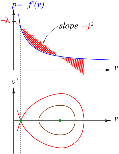
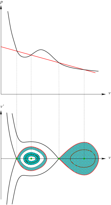
hence in particular is monotonically decaying to zero at infinity. The shallow water case is the main application we have in mind. If is to denote the endpoint of a solitary wave with and as constants of integration, it must satisfy
in which case there is exactly one other solution to Now, inside the homoclinic loop connecting to itself, there is a collection of periodic orbits surrounding , which are determined for instance by their trough (see Figure 1). More precisely, if there is a unique periodic orbit passing through and solving the ODE
Let us consider the mapping
with
It is a diffeomorphism onto the open subset of made of parameters for which we do have a periodic wave. From now on, we parametrize periodic waves by instead of . Given and there is a unique (the peak of the periodic wave) greater than such that
The wave number of the corresponding periodic wave is given by
and mean values can be computed by quadrature in a similar way. In particular, we have
An elegant way to remove (integrable) singularities at endpoints in the integrals above has been pointed out in [5]. Indeed, factorizing the denominator as
and introducing the change of variables
we find that
Note that in the shallow water case ,
hence is explicitly given by
First of all, we want to check whether (68)-(71) is an evolutionary system, or in other words if the Jacobian matrix of the mapping
is nonsingular. This can be done numerically. Next, we can rewrite (68)-(71) in the more compact form
from which we easily infer the quasilinear form
| (72) |
with , i.e.
By ‘change of frame’ , the hyperbolicity of (72) at is equivalent to the hyperbolicity of
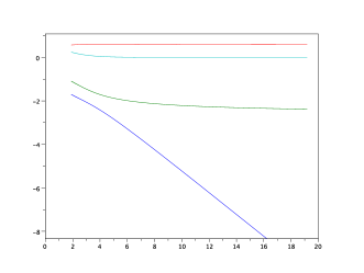
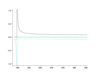
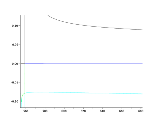
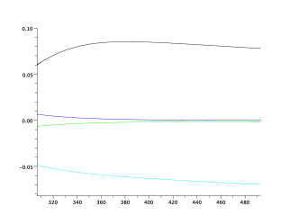
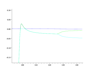
at . Once is known to be nonsingular, a sufficient condition for hyperbolicity is that the eigenvalues of have four distinct real parts, because then they must be real and distinct. We comment below on a series of numerical results obtained with the shallow water pressure law , in which we have computed mean values by using the trapezoidal rule with points of discretization, and the Jacobian matrices by means of a finite difference method and a discretization step . In each picture, we have plotted the real part of the eigenvalues of as a function of the period : the modulated equations are hyperbolic for a given if we find four distinct real parts. When two curves collide, there is a set of complex conjugate eigenvalue and the system is not hyperbolic any more.
4.1.2 Numerical results
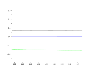
We have checked the hyperbolicity of the modulated equations in the cases and various values of and in the case , . Since the hyperbolicity does not depend on , we have set in and . In both cases we found a similar scenario. Let us describe the case . If , the Whitham equations are hyperbolic for all periodic waves (see figure 2).
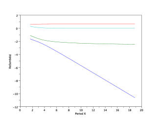
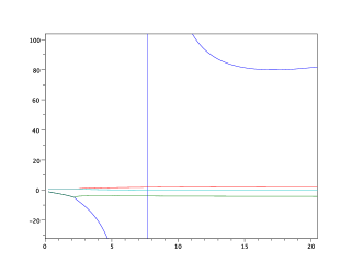
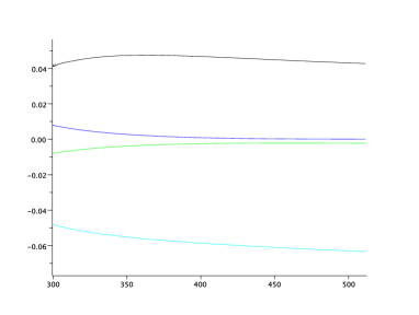
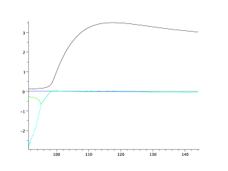
If , one finds a range of periodic wave periods for which the Whitham equations are not hyperbolic, and thus periodic waves are spectrally unstable; see figure 3 (left). Moreover, if , there is one eigenvalue that diverges to which means that there exists such that and the modulation equations are not of evolution type. If , the scenario is similar to the previous case: there is a range of unstable periodic waves; see figure 3 (right).

4.2 Van der Waals type pressure laws
4.2.1 Parametrization of periodic waves
We consider in this section pressure laws that are possibly nonconvex, and even nonmonotone. A typical example is the van der Waals pressure law
which exhibits various types of behaviors depending on the temperature (compared to , where is the perfect gas constant, and , , are parameters of the specific fluid). More precisely, defining
we easily see that
-
1.
for , is monotonically decaying and convex,
-
2.
for , is monotonically decaying and admits two inflection points,
-
3.
for , admits one local minimum, one local maximum, and two inflection points.
After nondimensionalization this pressure law reduces to
with . As seen above, transition values of are
and .
In what follows, we have chosen to deal with the case of a non monotone pressure and with and roughly corresponding to water,
so that .
If we choose such that , and take as in the previous subsection , the phase portrait of the travelling wave ODE
is certainly independent of the function , but heavily depends on the values of and when the pressure is non monotone.
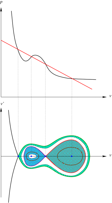
Depending on areas delimited by the pressure curve and by the so-called Rayleigh line, of equation in the plane, two typical phase portraits arise, which may be described as follows (see figure 4).
- Two fish
-
There are two disconnected homoclinic loops (the ‘fish’), one ending at and one with another endpoint, and all the trajectories outside these loops are unbounded; thus there are two types of periodic orbits, surrounded by either one of the homoclinic ones;
- Eyes-and-guitar
-
There are two homoclinic loops (the ‘eyes’) ending at the same point (maybe ), and a third homoclinic loop (the ‘guitar’) surrounds them; there are three types of periodic orbits, those inside the eyes, and those in between the eyes and the guitar.
A series of numerical investigations in various cases is reported below.
4.2.2 Numerical results in the eyes-and-guitar case
We have first considered the case , and checked the hyperbolicity of Whitham’s equations with a simple form of the capillary coefficient: . Here, we have an “eyes and guitar” type phase portrait. There are three families of periodic waves. The first one that is ‘above’ the doubly homoclinic orbit. In this case, there exists such that the modulation system is not of evolution type. Furthermore, there exists , such that if and , the modulated equations are hyperbolic and thus periodic waves are stable under large wavelength perturbations (see figure 5). On the other hand, we found that the periodic waves we could compute in the loops of the doubly homoclinic orbit are stable under large scale perturbations (here Whitham’s equations are hyperbolic); see figure 6. In the smallest loop, we stopped the computations at : below this value, the amplitude of periodic waves is too small in comparison to the precision we fixed. Anyway, as explained at the beginning, we expect that these periodic waves are unstable for sufficiently small amplitudes, since the Euler equations are not hyperbolic at the center point (pressure is nondecreasing at that point). We have tested and the situation is the same.
4.2.3 Numerical results in the two-fish case
Here, we have chosen and : in this case there are two separated homoclinic orbits. The first one is homoclinic to and the second one is homoclinic to . In this latter homoclinic, there is a center at from which bifurcates a family of periodic orbits. We have checked numerically the hyperbolicity of Whitham’s equations associated with this family: the modulation system is always hyperbolic (see figure 7).
In the homoclinic orbit to , there is a center at from which bifurcates the second family of periodic orbits. The picture is a bit more complicated: if , the modulation system is hyperbolic. Again, we stopped computations at in the smallest loop since amplitude of the waves are too small (for the precision of computations fixed here): it is expected that for sufficiently small amplitudes, periodic waves are unstable since the Euler equations are not hyperbolic there. Then if , the system is not hyperbolic and the associated periodic waves are unstable. Finally, if , the Whitham equations are hyperbolic again (see figure 8).
4.2.4 Conclusion from numerical investigations
We have found, in the cases where a doubly homoclinic orbit occurs, that periodic waves that are inside a homoclinic loop are always spectrally stable under long wave length perturbations or, more precisely, that the
modulation equations are hyperbolic. There is an additional family of periodic waves for which we observed that there is a critical period where the modulated equations are not of evolution type. Moreover, we found that there is such that Whitham’s equations are hyperbolic only if .
If there are two separated homoclinic orbits, we found that periodic waves which correspond to the larger solutions pass our stability test whereas there are range of periods where Whitham’s equations are not hyperbolic for the smaller solutions.
Appendix A A concrete computation
We derive here the averaged equations associated with Benjamin’s impulses and for (1) and (2) respectively. This computation is given for concreteness, even though it is contained in the abstract computation made in Section 2. Taking the inner product of (41) and (42) with and respectively, then averaging and integrating by parts in , we receive
All terms with index one here above cancel out because of the profile equations (39) and (40), which imply indeed that
This is straightforward for the equations on the left, and for the ones on the right we observe that the second order differential operators and have been defined in such a way that
Finally, we recover the equations in (50) and (52) obtained by averaging the impulses’ conservation laws by checking that
Let us check the first equality, the second one being identical through the symmetry . We have
Recalling the definition of and integrating once by parts (in of course), we get
So it just remains to show that
Once again, this follows from integrations by parts. Indeed,
Appendix B A convenient structural assumption
Our purpose here is to check that, under a reasonable structure assumption on the Hamiltonian , the operator behaves properly, and if the kernel of has the expected size, our parametrization hypothesis for periodic profiles is met.
Structure of the Hamiltonian
To go further into the analysis of the abstract equation (5), we need to be more specific about the form of the Hamiltonian . Inspired by our examples (1)(3), (2)(4), and (9), we write the -space as for some integer , , require that
and assume that is uniformly strongly convex in both and on the range of -values and speeds under consideration. Note that a simple way to make this assumption independent of is to assume that has a block structure of the form
as is the case for the Euler-Korteweg system.
B.1 Compactness of resolvents
We briefly sketch here a proof of the fact that our structural assumption on ensures that with domain have a nonempty resolvent set and compact resolvents. In turn, this implies that, for all , is a relatively compact perturbation of .
Our structural assumptions readily yield
with , ,
with and being uniformly positive definite. Then, standard energy estimates enable us to show that
where is a positive constant independent of . From this we obtain that there exist and such that if then
| (73) |
This already shows that, for such a , has a closed range and is one-to-one with a continuous inverse. To check that the previous range is dense, we only need to examine whether the formal adjoint is indeed one-to-one (on smooth functions). This amounts to show that
| (74) |
has no nontrivial smooth solution . Applying the operator to (74), we deduce from (73) applied to and that , which in turn implies , because of (74) and the fact that is nonzero. This proves that for the above , if then lies in the resolvent set of .
Since we have not used any Poincaré inequality in our previous arguments, they apply mutatis mutandis to with domain , and show that it has a nonempty resolvent set.
B.2 Parametrization of periodic orbits
Let us prove that, under our structural assumption on , there is no restriction in assuming, as done in Theorem 1, that Whitham’s parametrization by is admissible. More precisely, we are going to show that, if nearby periodic traveling wave profiles form a dimensional manifold, and if the generalized kernel of is of dimension , then those nearby profiles are parametrized by . This extends to our Hamiltonian framework a result previously shown for parabolic conservation laws by Serre [19].
To set things on a more formal ground, we define on some open neighborhood of wave values the map
where denotes the jump , and is the solution of
We identify in the usual way nearby periodic traveling wave profiles with elements of the zero set of .
Proposition 2.
Assume that is non trivial and that has constant rank . Then the generalized kernel of is of dimension if and only if, up to translation, nearby periodic traveling wave profiles may be regularly parametrized by .
Proof.
Our proof is based upon the fact that the dimension of the generalized kernel of is the algebraic multiplicity of zero as a root of some Evans function (see [11]). Indeed, viewing spectral problem
| (75) |
for as a system of coupled differential equations of third-order in and first-order in , we may introduce its fundamental solution normalized by and define
Then the condition on the dimension of the generalized kernel of reads
for some nonzero [11]. We want to convert this into some information about profiles parametrization.
Let us denote by the solution to (75) corresponding to the -th column of the matrix , that is solves (75) and is the -th vector of the canonical basis of . The Evans function is then written
where we have dropped the marks and on jumps. To go further, using our structural assumptions, we write333We warn the reader that, because of factors, these notations are not compatible with the ones of the previous section of the present Appendix.
with , ,
and being uniformly positive definite. Integrating (75) from to yields
Therefore, up to a nonzero multiplicative constant, is also written
Now, corresponding to the impulse equation, we also have
where the convention is as before that linearization and derivatives are taken at . By integrating the relation here above, we obtain
We still need to check that it is not a trivial relation. But, since is non trivial, there is a point where is nonzero, otherwise would be constant thus and would also be constant, a contradiction. Then, since assumptions of the proposition and terms of the equivalence we are currently proving are invariant by translation, we may assume that is nonzero. Now let us pick such that the -th component of is nonzero and, for any , denote by the vector of obtained from by deleting the -th component. Then, up to a nonzero multiplicative constant, is
Up to a change of basis we may assume that , for and is a basis of the linear span of . With this choice, after setting , is written up to a nonzero multiplicative constant
Since satisfies , it differs from by an element of the kernel of which is spanned by . This yields that, up to a multiplicative nonzero constant and an additive remainder , reads
or
We are ready to complete the proof by observing the latter determinant. Indeed our assumption on implies that the -st rows of the above matrix are linearly independent. Furthermore, the kernel of the corresponding linear map is the tangent space at of the profiles manifold (profiles being identified when equal up to translation). Thus the differential map of is invertible on this tangent space if and only if the above determinant is non zero. Consequently, this map is full-rank if and only if the generalized kernel of is of dimension . ∎
Appendix C Galilean invariance
In order to check that the hyperbolicity of the Euler–Korteweg modulation equations (53) does not depend on , it is convenient to rewrite those equations in a form that is similar to (66) for (55). Substituting for the mean momentum in (53), and manipulating the remaining mean values as in the proof of Theorem 2, we receive the system
| (76) |
together with the generalized Gibbs relation (62) . Then, we easily check that (76) is invariant by the Galilean transformation
for any . Since this transformation leaves invariant all the ‘thermodynamic’ variables , it leaves (76) invariant just because it does so for the reduced system
Acknowledgement.
This work has been partly supported by the European Research Council \hrefhttp://math.univ-lyon1.fr/ filbet/nusikimo/nusikimo.htmERC Starting Grant 2009, project 239983- NuSiKiMo.
References
- [1] J. Angulo Pava. Nonlinear dispersive equations, volume 156 of Mathematical Surveys and Monographs. American Mathematical Society, Providence, RI, 2009. Existence and stability of solitary and periodic travelling wave solutions.
- [2] T. B. Benjamin. Impulse, flow force and variational principles. IMA J. Appl. Math., 32(1-3):3–68, 1984.
- [3] S. Benzoni Gavage. Planar traveling waves in capillary fluids. Differential Integral Equations, 26(3-4):433Ð478, 2013.
- [4] Nate Bottman and Bernard Deconinck. KdV cnoidal waves are spectrally stable. Discrete Contin. Dyn. Syst., 25(4):1163–1180, 2009.
- [5] J. C. Bronski and M. A. Johnson. The modulational instability for a generalized Korteweg-de Vries equation. Arch. Ration. Mech. Anal., 197(2):357–400, 2010.
- [6] J. C. Bronski, M. A. Johnson, and T. Kapitula. An index theorem for the stability of periodic traveling waves of Korteweg-de Vries type. Proc. Roy. Soc. Edinburgh Sect. A, 141(6):1141–1173, 2011.
- [7] A. Doelman, B. Sandstede, A. Scheel, and G. Schneider. The dynamics of modulated wave trains. Mem. Amer. Math. Soc., 199(934):viii+105, 2009.
- [8] G. A. El. Resolution of a shock in hyperbolic systems modified by weak dispersion. Chaos, 15(3):037103, 21, 2005.
- [9] G. A. El, R. H. J. Grimshaw, and N. F. Smyth. Unsteady undular bores in fully nonlinear shallow-water theory. Physics of Fluids, 18(2):027104, February 2006.
- [10] Th. Gallay and M. Hărăguş. Stability of small periodic waves for the nonlinear Schrödinger equation. J. Differential Equations, 234(2):544–581, 2007.
- [11] R. A. Gardner. On the structure of the spectra of periodic travelling waves. J. Math. Pures Appl. (9), 72(5):415–439, 1993.
- [12] S. L. Gavrilyuk and D. Serre. A model of a plug-chain system near the thermodynamic critical point: connection with the Korteweg theory of capillarity and modulation equations. In Waves in liquid/gas and liquid/vapour two-phase systems (Kyoto, 1994), volume 31 of Fluid Mech. Appl., pages 419–428. Kluwer Acad. Publ., Dordrecht, 1995.
- [13] J. Höwing. Stability of large- and small-amplitude solitary waves in the generalized Korteweg-de Vries and Euler-Korteweg / Boussinesq equations. J. Differential Equations, 251(9):2515–2533, 2011.
- [14] M. A. Johnson, K. Zumbrun, and J. C. Bronski. On the modulation equations and stability of periodic generalized Korteweg-de Vries waves via Bloch decompositions. Phys. D, 239(23-24):2057–2065, 2010.
- [15] M.A. Johnson, P. Noble, L.M. Rodrigues, and K. Zumbrun. Behavior of periodic solutions of viscous conservation laws under localized and nonlocalized perturbations. arXiv:1211.2156, 2012.
- [16] T. Kato. Perturbation theory for linear operators. Springer-Verlag New York, Inc., New York, 1966. Die Grundlehren der mathematischen Wissenschaften, Band 132.
- [17] M. Oh and K. Zumbrun. Stability of periodic solutions of conservation laws with viscosity: analysis of the Evans function. Arch. Ration. Mech. Anal., 166(2):99–166, 2003.
- [18] M. Oh and K. Zumbrun. Stability of periodic solutions of conservation laws with viscosity: pointwise bounds on the Green function. Arch. Ration. Mech. Anal., 166(2):167–196, 2003.
- [19] D. Serre. Spectral stability of periodic solutions of viscous conservation laws: large wavelength analysis. Comm. Partial Differential Equations, 30(1-3):259–282, 2005.
- [20] G. B. Whitham. Two-timing, variational principles and waves. J. Fluid Mech., 44:373–395, 1970.
- [21] G. B. Whitham. Linear and nonlinear waves. John Wiley & Sons Inc., New York, 1999. Reprint of the 1974 original, A Wiley-Interscience Publication.