Abstract: We describe an algorithm to construct an intrinsic Delaunay triangulation of a smooth closed submanifold of Euclidean space. Using results established in a companion paper on the stability of Delaunay triangulations on $\delta$-generic point sets, we establish sampling criteria which ensure that the intrinsic Delaunay complex coincides with the restricted Delaunay complex and also with the recently introduced tangential Delaunay complex. The algorithm generates a point set that meets the required criteria while the tangential complex is being constructed. In this way the computation of geodesic distances is avoided, the runtime is only linearly dependent on the ambient dimension, and the Delaunay complexes are guaranteed to be triangulations of the manifold.

Key-words: Delaunay triangulation, submanifolds, Riemannian geometry

Construire des triangulations de Delaunay intrinsèque pour les sous-variétés

Résumé : Nous montrons que, pour toute sous variété M suffisamment régulière de l’espace euclidien et pour tout échantillon P de points de M qui satisfait une condition locale de delta-généricité et de epsilon-densité, P admet une triangulation de Delaunay intrinsèque qui est égale à la triangulation de Delaunay restreinte à M et aussi au complexe de Delaunay tangent. Nous montrons également comment produire de tels ensembles de points.

Mots-clés : triangulation de Delaunay, sous-variétés, géométrie riemannienne

1 Introduction

This paper addresses the problem of constructing an intrinsic Delaunay triangulation of a smooth closed submanifold $\mathcal{M}\subset\mathbb{R}^{N}$. We present an algorithm which generates a point set $\mathcal{P}\subset\mathcal{M}$ and a simplicial complex on $\mathcal{P}$ that is homeomorphic to $\mathcal{M}$ and has a connectivity determined by the Delaunay triangulation of $\mathcal{P}$ with respect to the intrinsic metric of $\mathcal{M}$.

For a submanifold of Euclidean space, the restricted Delaunay complex [ES97], which is defined by the ambient metric restricted to the submanifold, was employed by Cheng et al. [CDR05] as the basis for a triangulation. However, it was found that sampling density alone was insufficient to ensure a triangulation, and manipulations of the complex were employed.

In an earlier work, Leibon and Letscher [LL00] announced sampling density conditions which would ensure that the Delaunay complex defined by the intrinsic metric of the manifold was a triangulation. In fact, as shown in Section 2.4.3 and Appendix A, the stated result is incorrect: sampling density alone is insufficient to guarantee an intrinsic Delaunay triangulation (see Theorem A.3). Topological defects can arise when the vertices lie too close to a degenerate or “quasi-cospherical” configuration.

Our interest in the intrinsic Delaunay complex stems from its close relationship with other Delaunay-like structures that have been proposed in the context of non-homogeneous metrics. For example, anisotropic Voronoi diagrams [LS03] and anisotropic Delaunay triangulations emerge as natural structures when we want to mesh a domain of $\mathbb{R}^{m}$ while respecting a given metric tensor field.

This paper builds over preliminary results on anisotropic Delaunay meshes [BWY11] and manifold reconstruction using the tangential Delaunay complex [BG11]. The central idea in both cases is to define Euclidean Delaunay triangulations locally and to glue these local triangulations together by removing inconsistencies between them. We view the inconsistencies as arising from instability in the Delaunay triangulations, and exploit the results of a companion paper [BDG12] to define sampling conditions under which these inconsistencies cannot arise.

The algorithm is based on the tangential Delaunay complex [BG11], and is an adaptation of a Delaunay refinement algorithm designed to avoid poorly shaped “sliver” simplices [Li03, BG10]. The tangential Delaunay complex is defined with respect to local Delaunay triangulations restricted to the tangent spaces at sample points. We demonstrate that the algorithm produces sampling conditions such that the tangential Delaunay complex coincides with the restricted Delaunay complex and the intrinsic Delaunay complex. The refinement algorithm avoids the problem of slivers without the need to resort to a point weighting strategy [CDE⁺00, CDR05, BG11], which alters the definition of the restricted Delaunay complex.

We present background and foundational material in Section 2. Then, in Section 3, we exploit results established in [BDG12] to demonstrate sampling conditions under which the intrinsic Delaunay complex, the restricted Delaunay complex, and the tangential Delaunay complex coincide and are manifold. The algorithm itself is presented in Section 4, and the analysis of the algorithm is presented in Section 5.

2 Background

Within the context of the standard $m$-dimensional Euclidean space $\mathbb{R}^{m}$, when distances are determined by the standard norm, $\left\|\cdot\right\|$, we use the following conventions. The distance between a point $p$ and a set $X\subset\mathbb{R}^{m}$, is the infimum of the distances between $p$ and the points of $X$, and is denoted $d_{\mathbb{R}^{m}}(p,X)$. We refer to the distance between two points $a$ and $b$ as $\left\|b-a\right\|$ or $d_{\mathbb{R}^{m}}(a,b)$ as convenient. A ball $B_{\mathbb{R}^{m}}(c,r)=\{x\,|\,\left\|x-c\right\|<r\}$ is open, and $\overline{B}_{\mathbb{R}^{m}}(c,r)$ is its topological closure. Generally, we denote the topological closure of a set $X$ by $\overline{X}$, the interior by $\operatorname{int}(X)$, and the boundary by $\partial{X}$. The convex hull is denoted $\operatorname{conv}(X)$, and the affine hull is $\operatorname{aff}(X)$.

We will make use of other metrics besides the Euclidean one. A generic metric is denoted $d$, and the associated open and closed balls are $B(c,r)$, and $\overline{B}(c,r)$. If a specific metric is intended, it will be indicated by a subscript, for example in Section 3 we introduce $d_{\mathcal{M}}$, the intrinsic metric on a manifold $\mathcal{M}$, which has associated balls $B_{\mathcal{M}}(c,r)$.

If $A$ is a $k\times j$ matrix, we denote its $i^{th}$ singular value by $s_{i}(A)$. We use the operator norm $\left\|A\right\|=s_{1}(A)=\sup_{\left\|x\right\|=1}\left\|Ax\right\|$.

If $U$ and $V$ are vector subspaces of $\mathbb{R}^{m}$, with $\dim U\leq\dim V$, the angle between them is defined by

$$\sin\angle(U,V)=\sup_{u\in U}\left\|u-\pi_{V}u\right\|,$$

where $\pi_{V}$ is the orthogonal projection onto $V$. This is the largest principal angle between $U$ and $V$. The angle between affine subspaces $K$ and $H$ is defined as the angle between the corresponding parallel vector subspaces.

2.1 Sampling parameters and perturbations

The structures of interest will be built from a finite set $\mathsf{P}\subset\mathbb{R}^{m}$, which we consider to be a set of sample points. If $D\subset\mathbb{R}^{m}$ is a bounded set, then $\mathsf{P}$ is an $\epsilon$-sample set for $D$ if $d_{\mathbb{R}^{m}}(x,\mathsf{P})<\epsilon$ for all $x\in\overline{D}$. We say that $\epsilon$ is a sampling radius for $D$ satisfied by $\mathsf{P}$. If no domain $D$ is specified, we say $\mathsf{P}$ is an $\epsilon$-sample set if $d(x,\mathsf{P}\cup\partial{\operatorname{conv}(\mathsf{P})})<\epsilon$ for all $x\in\operatorname{conv}(\mathsf{P})$. Equivalently, $\mathsf{P}$ is an $\epsilon$-sample set if it satisfies a sampling radius $\epsilon$ for

$$D_{\epsilon}(\mathsf{P})=\{x\in\operatorname{conv}(\mathsf{P})\,|\,d_{\mathbb{R}^{m}}(x,\partial{\operatorname{conv}(\mathsf{P})})\geq\epsilon\}.$$

In particular, if $\mathcal{P}$ is an $\epsilon$-sample set for $U$, and $\mathsf{P}=U\cap\mathcal{P}$, and $\operatorname{conv}(\mathsf{P})\subset U$, then $\mathsf{P}$ is an $\epsilon$-sample set.

A set $\mathsf{P}$ is $\lambda$-sparse if $d_{\mathbb{R}^{m}}(p,q)>\lambda$ for all $p,q\in\mathsf{P}$. We usually assume that the sparsity of a $\epsilon$-sample set is proportional to $\epsilon$, thus: $\lambda=\mu_{0}\epsilon$.

We consider a perturbation of the points $\mathsf{P}\subset\mathbb{R}^{m}$ given by a function $\zeta:\mathsf{P}\to\mathbb{R}^{m}$. If $\zeta$ is such that $d_{\mathbb{R}^{m}}(p,\zeta(p))\leq\rho$, we say that $\zeta$ is a $\rho$-perturbation. As a notational convenience, we frequently define $\tilde{\mathsf{P}}=\zeta(\mathsf{P})$, and let $\tilde{p}$ represent $\zeta(p)\in\tilde{\mathsf{P}}$. We will only be considering $\rho$-perturbations where $\rho$ is less than half the sparsity of $\mathsf{P}$, so $\zeta:\mathsf{P}\to\tilde{\mathsf{P}}$ is a bijection.

Points in $\mathsf{P}$ which are not on the boundary of $\operatorname{conv}(\mathsf{P})$ are interior points of $\mathsf{P}$.

2.2 Simplices

Given a set of $j+1$ points $\{p_{0},\ldots,p_{j}\}\subset\mathsf{P}\subset\mathbb{R}^{m}$, a (geometric) $j$-simplex $\sigma=[p_{0},\ldots,p_{j}]$ is defined by the convex hull: $\sigma=\operatorname{conv}(\{p_{0},\ldots,p_{j}\})$. The points $p_{i}$ are the vertices of $\sigma$. Any subset $\{p_{i_{0}},\ldots,p_{i_{k}}\}$ of $\{p_{0},\ldots,p_{j}\}$ defines a $k$-simplex $\tau$ which we call a face of $\sigma$. We write $\tau\leq\sigma$ if $\tau$ is a face of $\sigma$, and $\tau<\sigma$ if $\tau$ is a proper face of $\sigma$, i.e., if the vertices of $\tau$ are a proper subset of the vertices of $\sigma$.

The boundary of $\sigma$, is the union of its proper faces: $\partial{\sigma}=\bigcup_{\tau<\sigma}\tau$. In general this is distinct from the topological boundary defined above, but we denote it with the same symbol. The interior of $\sigma$ is $\operatorname{int}(\sigma)=\sigma\setminus\partial{\sigma}$. Again this is generally different from the topological interior. Other geometric properties of $\sigma$ include its diameter (the length of its longest edge), $\Delta(\sigma)$, and the length of its shortest edge, $L(\sigma)$. If $\sigma$ is a $0$-simplex, we define $L(\sigma)=\Delta(\sigma)=0$.

For any vertex $p\in\sigma$, the face oppposite $p$ is the face determined by the other vertices of $\sigma$, and is denoted $\sigma_{p}$. If $\tau$ is a $j$-simplex, and $p$ is not a vertex of $\tau$, we may construct a $(j+1)$-simplex $\sigma={p}*{\tau}$, called the join of $p$ and $\tau$. It is the simplex defined by $p$ and the vertices of $\tau$, i.e., $\tau=\sigma_{p}$.

Our definition of a simplex has made an important departure from standard convention: we do not demand that the vertices of a simplex be affinely independent. A $j$-simplex $\sigma$ is a degenerate simplex if $\dim\operatorname{aff}(\sigma)<j$. If we wish to emphasise that a simplex is a $j$-simplex, we write $j$ as a superscript: $\sigma^{j}$; but this always refers to the combinatorial dimension of the simplex.

If $\sigma$ is non-degenerate, then it has a circumcentre, $C(\sigma)$, which is the centre of the smallest circumscribing ball for $\sigma$. The radius of this ball is the circumradius of $\sigma$, denoted $R(\sigma)$. A degenerate simplex may or may not have a circumcentre and circumradius. We write $R(\sigma)$ to indicate that a simplex has a circumcentre. We will make use of the affine space $N(\sigma)$ composed of the centres of the balls that circumscribe $\sigma$. We sometimes refer to a point $c\in N(\sigma)$ as a centre for $\sigma$. The space $N(\sigma)$ is orthogonal to $\operatorname{aff}(\sigma)$ and intersects it at the circumcentre of $\sigma$. Its dimension is $m-\dim\operatorname{aff}(\sigma)$.

The altitude of $p$ in $\sigma$ is $D(p,\sigma)=d_{\mathbb{R}^{m}}(p,\operatorname{aff}(\sigma_{p}))$. A poorly-shaped simplex can be characterized by the existence of a relatively small altitude. The thickness of a $j$-simplex $\sigma$ is the dimensionless quantity

$$\Upsilon(\sigma)=\begin{cases}1&\text{if $j=0$}\\ \min_{p\in\sigma}\frac{D(p,\sigma)}{j\Delta(\sigma)}&\text{otherwise.}\end{cases}$$

We say that $\sigma$ is $\Upsilon_{0}$-thick, if $\Upsilon(\sigma)\geq\Upsilon_{0}$. If $\sigma$ is $\Upsilon_{0}$-thick, then so are all of its faces. Indeed if $\tau\leq\sigma$, then the smallest altitude in $\tau$ cannot be smaller than that of $\sigma$, and also $\Delta(\tau)\leq\Delta(\sigma)$.

Although he worked with volumes rather than altitudes, Whitney [Whi57, p. 127] proved that the affine hull of a thick simplex makes a small angle with any hyperplane which lies near all the vertices of the simplex. We can state this [BDG12, Lemma 2.5] as:

Lemma 2.1 (Whitney angle bound).

Suppose $\sigma$ is a $j$-simplex whose vertices all lie within a distance $\eta$ from a $k$-dimensional affine space, $H\subset\mathbb{R}^{m}$, with $k\geq j$. Then

$$\sin\angle(\operatorname{aff}(\sigma),H)\leq\frac{2\eta}{\Upsilon(\sigma)\Delta(\sigma)}.$$

2.2.1 Simplex perturbation

We will make use of two results displaying the robustness of thick simplices with respect to small perturbations of their vertices. The first observation bounds the change in thickness itself under small perturbations:

Lemma 2.2 (Thickness under perturbation).

Let $\sigma=[p_{0},\ldots,p_{j}]$ and $\tilde{\sigma}=[\tilde{p}_{0},\ldots,\tilde{p}_{j}]$ be $j$-simplices such that $\left\|\tilde{p}_{i}-p_{i}\right\|\leq\rho$ for all $i\in\{0,\ldots,j\}$. For any positive $\eta\leq 1$, if

$$\rho\leq\frac{(1-\eta)\Upsilon(\sigma)^{2}L(\sigma)}{14},$$ (1)

then

$$D(\tilde{p}_{i},\tilde{\sigma})\geq\eta D(p_{i},\sigma),$$

for all $i\in\{0,\ldots,j\}$. It follows that

$$\Upsilon(\tilde{\sigma})\Delta(\tilde{\sigma})\geq\eta\Upsilon(\sigma)\Delta(\sigma),$$

and

$$\Upsilon(\tilde{\sigma})\geq\left(1-\frac{2\rho}{\Delta(\sigma)}\right)\eta\Upsilon(\sigma)\geq\frac{6}{7}\eta\Upsilon(\sigma).$$

Proof.

Let $p,q\in\sigma$ with $\tilde{p},\tilde{q}$ the corresponding vertices of $\tilde{\sigma}$. Let $v=p-q$ and $\tilde{v}=\tilde{p}-\tilde{q}$. Define $\theta=\angle(v,\operatorname{aff}(\sigma_{p}))$ and $\tilde{\theta}=\angle(\tilde{v},\operatorname{aff}(\tilde{\sigma}_{\tilde{p}}))$. Since $\Upsilon(\sigma)\leq\Upsilon(\sigma_{p})$, Whitney’s Lemma 2.1 lets us bound $\angle(\operatorname{aff}(\sigma_{p}),\operatorname{aff}(\tilde{\sigma}_{\tilde{p}}))$ by the angle $\alpha$ defined by

$$\sin\alpha=\frac{2\rho}{\Upsilon(\sigma){\Delta(\sigma)}}.$$

Also, by an elementary geometric argument,

$$\sin\gamma=\frac{2\rho}{\left\|v\right\|}$$

defines $\gamma$ as an upper bound on the angle between the lines generated by $v$ and $\tilde{v}$.

Thus we have

$$D(\tilde{p},\tilde{\sigma})=\left\|\tilde{v}\right\|\sin\tilde{\theta}\geq(\left\|v\right\|-2\rho)\sin(\theta-\alpha-\gamma).$$

Using the addition formula for sine together with the facts that for $x,y\in[0,\frac{\pi}{2}]$, $(1-x)\leq\cos x$; $2\sin x\geq x$; and $\sin x+\sin y\geq\sin(x+y)$, we get

$$D(\tilde{p},\tilde{\sigma})\geq(\left\|v\right\|-2\rho)\left[\left(1-2\left(\frac{2\rho}{\Upsilon(\sigma)\Delta(\sigma)}+\frac{2\rho}{\left\|v\right\|}\right)\right)\frac{D(p,\sigma)}{\left\|v\right\|}-\left(\frac{2\rho}{\Upsilon(\sigma)\Delta(\sigma)}+\frac{2\rho}{\left\|v\right\|}\right)\right].$$

For convenience, define $\mu=\frac{2\rho}{L(\sigma)}\geq\frac{2\rho}{\left\|v\right\|}\geq\frac{2\rho}{\Delta(\sigma)}$. Then

$$\begin{split}D(\tilde{p},\tilde{\sigma})&\geq\left\|v\right\|(1-\mu)\left[\left(1-2\left(1+\frac{1}{\Upsilon(\sigma)}\right)\mu\right)\frac{D(p,\sigma)}{\left\|v\right\|}-\left(1+\frac{1}{\Upsilon(\sigma)}\right)\mu\right]\\ &\geq(1-\mu)\left[\left(1-\frac{4\mu}{\Upsilon(\sigma)}\right)D(p,\sigma)-\frac{2\mu\left\|v\right\|}{\Upsilon(\sigma)}\right]\\ &\geq(1-\mu)\left[\left(1-\frac{4\mu}{\Upsilon(\sigma)}\right)D(p,\sigma)-\frac{2\mu\left\|v\right\|}{\Upsilon(\sigma)^{2}\Delta(\sigma)}D(p,\sigma)\right]\\ &\geq(1-\mu)\left(1-\frac{4\mu}{\Upsilon(\sigma)}-\frac{2\mu}{\Upsilon(\sigma)^{2}}\right)D(p,\sigma)\\ &\geq\left(1-\frac{7\mu}{\Upsilon(\sigma)^{2}}\right)D(p,\sigma)\\ &\geq KD(p,\sigma)\qquad\qquad\text{ when }\mu\leq\frac{(1-K)\Upsilon(\sigma)^{2}}{7}.\end{split}$$

The condition on $\mu$ is satisfied when $\rho$ satisfies Inequality (1).

The bound on $\Upsilon(\tilde{\sigma})\Delta(\tilde{\sigma})$ follows immediately from the bounds on the $D(\tilde{p},\tilde{\sigma})$, and the bound on $\Upsilon(\tilde{\sigma})$ itself follows from the observation that

$$\frac{\Delta(\sigma)}{\Delta(\tilde{\sigma})}\geq\frac{\Delta(\sigma)}{\Delta(\sigma)+2\rho}\geq\left(1-\frac{2\rho}{\Delta(\sigma)}\right)\geq\left(1-\frac{\Upsilon(\sigma)^{2}}{7}\right)\geq\frac{6}{7},$$

when $\rho$ satisfies Inequality (1).

We will also make use of a bound relating circumscribing balls of a simplex that undergoes a perturbation:

Lemma 2.3 (Circumscribing balls under perturbation).

Let $\sigma=[p_{0},\ldots,p_{j}]$ and $\tilde{\sigma}=[\tilde{p}_{0},\ldots,\tilde{p}_{j}]$ be $j$-simplices such that $\left\|\tilde{p}_{i}-p_{i}\right\|\leq\rho$ for all $i\in\{0,\ldots,j\}$. Suppose $B=B_{\mathbb{R}^{m}}(c,r)$, with $r<\epsilon$, is a circumscribing ball for $\sigma$. If

$$\rho\leq\frac{\Upsilon(\sigma)^{2}L(\sigma)}{28},$$

then there is a circumscribing ball $\tilde{B}=B_{\mathbb{R}^{d}}(\tilde{c},\tilde{r})$ for $\tilde{\sigma}$ with

$$\left\|\tilde{c}-c\right\|<\left(\frac{8\epsilon}{\Upsilon(\sigma)\Delta(\sigma)}\right)\rho$$ (2)

and

$$\left|\tilde{r}-r\right|<\left(\frac{9\epsilon}{\Upsilon(\sigma)\Delta(\sigma)}\right)\rho.$$

If, in addition, we have that $\tilde{p}_{0}=p_{0}$, then $\left|\tilde{r}-r\right|\leq\left\|\tilde{c}-c\right\|$, and (2) serves also as a bound on $\left|\tilde{r}-r\right|$.

Proof.

By the perturbation bounds, the distances between $c$ and the vertices of $\tilde{\sigma}$ differ by no more than $2\rho$. Also, $\left\|c-p_{i}\right\|<\tilde{\epsilon}=\epsilon+\rho$, and so by [BDG12, Lemma 4.3] we have

$$d_{\mathbb{R}^{m}}(c,N(\tilde{\sigma}))<\frac{2\tilde{\epsilon}\rho}{\Upsilon(\tilde{\sigma})\Delta(\tilde{\sigma})}.$$

The bound on $\rho$ allows us to apply Lemma 2.2 with $K=\frac{1}{2}$, so $\Upsilon(\tilde{\sigma})\Delta(\tilde{\sigma})\geq\frac{1}{2}\Upsilon(\sigma)\Delta(\sigma)$, and we obtain the bound on $\left\|\tilde{c}-c\right\|$ with the observation that $\tilde{\epsilon}\leq 2\epsilon$. Indeed, $\rho\leq\epsilon$ because $L(\sigma)\leq 2\epsilon$.

By the triangle inequality $\left|\tilde{r}-r\right|\leq\left\|\tilde{p}_{0}-p_{0}\right\|+\left\|\tilde{c}-c\right\|$, and the stated bound on $\left|\tilde{r}-r\right|$ follows from the observation that $\frac{\epsilon}{\Upsilon(\sigma)\Delta(\sigma)}\geq 1$ if $j>1$. Under the assumption that $\tilde{p}_{0}=p_{0}$, the bound on $\left\|\tilde{c}-c\right\|$ also serves as a bound on $\left|\tilde{r}-r\right|$.

2.2.2 Flakes

For algorithmic reasons, it is convenient to have a more structured constraint on simplex geometry than that provided by a simple thickness bound. A simplex that is not thick has a relatively small altitude, but we wish to exploit a family of bad simplices for which all the altitudes are relatively small. As shown by Lemma 2.7 below, the $\Gamma_{0}$-flakes form such a family. The flake parameter $\Gamma_{0}$ is a positive real number smaller than one.

Definition 2.4 ($\Gamma_{0}$-good simplices and $\Gamma_{0}$-flakes).

A simplex $\sigma$ is $\Gamma_{0}$-good if $\Upsilon(\sigma^{j})\geq\Gamma_{0}^{j}$ for all $j$-simplices $\sigma^{j}\leq\sigma$. A simplex is $\Gamma_{0}$-bad if it is not $\Gamma_{0}$-good. A $\Gamma_{0}$-flake is a $\Gamma_{0}$-bad simplex in which all the proper faces are $\Gamma_{0}$-good.

Observe that a flake must have dimension at least $2$, since $\Upsilon(\sigma^{j})=1$ for $j<2$. A flake that has an upper bound on the ratio of its circumradius to its shortest edge is called a sliver. The flakes we will be considering have no upper bound on their circumradius, and in fact they may be degenerate and not even have a circumradius.

Ensuring that all simplices are $\Gamma_{0}$-good is the same as ensuring that there are no flakes. Indeed, if $\sigma$ is $\Gamma_{0}$-bad, then it has a $j$-face $\sigma^{j}\leq\sigma$ that is not $\Gamma_{0}^{j}$-thick. By considering such a face with minimal dimension we arrive at the following important observation:

Lemma 2.5.

A simplex is $\Gamma_{0}$-bad if and only if it has a face that is a $\Gamma_{0}$-flake.

We obtain an upper bound on the altitudes of a $\Gamma_{0}$-flake through a consideration of dihedral angles. In particular, we observe the following general relationship between simplex altitudes:

Lemma 2.6.

If $\sigma$ is a $j$-simplex with $j\geq 2$, then for any two vertices $p,q\in\sigma$, the dihedral angle between $\sigma_{p}$ and $\sigma_{q}$ defines an equality between ratios of altitudes:

$$\sin\angle(\operatorname{aff}(\sigma_{p}),\operatorname{aff}(\sigma_{q}))=\frac{D(p,\sigma)}{D(p,\sigma_{q})}=\frac{D(q,\sigma)}{D(q,\sigma_{p})}.$$

Proof.

Let $\sigma_{pq}=\sigma_{p}\cap\sigma_{q}$, and let $p_{*}$ be the projection of $p$ into $\operatorname{aff}(\sigma_{pq})$. Taking $p_{*}$ as the origin, we see that $\frac{p-p_{*}}{D(p,\sigma_{q})}$ has the maximal distance to $\operatorname{aff}(\sigma_{p})$ out of all the unit vectors in $\operatorname{aff}(\sigma_{q})$, and this distance is $\frac{D(p,\sigma)}{D(p,\sigma_{q})}$. By definition this is the sine of the angle between $\operatorname{aff}(\sigma_{p})$ and $\operatorname{aff}(\sigma_{q})$. A symmetric argument is carried out with $q$ to obtain the result.

We arrive at the following important observation about flake simplices:

Lemma 2.7 (Flakes have small altitudes).

If a $k$-simplex $\sigma$ is a $\Gamma_{0}$-flake, then for every vertex $p\in\sigma$, the altitude satisfies the bound

$$D(p,\sigma)<\frac{k\Delta(\sigma)^{2}\Gamma_{0}}{(k-1)L(\sigma)}.$$

Proof.

Recalling Lemma 2.6 we have

$$D(p,\sigma)=\frac{D(q,\sigma)D(p,\sigma_{q})}{D(q,\sigma_{p})},$$

and taking $q$ to be a vertex with minimal altitude, we have

$$D(q,\sigma)=k\Upsilon(\sigma)\Delta(\sigma)<k\Gamma_{0}^{k}\Delta(\sigma),$$

and

$$D(q,\sigma_{p})\geq(k-1)\Upsilon(\sigma_{p})\Delta(\sigma_{p})\geq(k-1)\Gamma_{0}^{k-1}L(\sigma),$$

and

$$D(p,\sigma_{q})\leq\Delta(\sigma_{q})\leq\Delta(\sigma),$$

and the bound is obtained.

2.3 Complexes

Given a finite set $\mathsf{P}$, an abstract simplicial complex is a set of subsets $K\subset 2^{\mathsf{P}}$ such that if $\sigma\in K$, then every subset of $\sigma$ is also in $K$. The Delaunay complexes we study are abstract simplicial complexes, but their simplices carry a canonical geometry induced from the inclusion map $\iota:\mathsf{P}\hookrightarrow\mathbb{R}^{m}$. (We assume $\iota$ is injective on $\mathsf{P}$, and so do not distinguish between $\mathsf{P}$ and $\iota(\mathsf{P})$.) To each abstract simplex $\sigma\in K$, we have an associated geometric simplex $\operatorname{conv}(\iota(\sigma))$, and normally when we write $\sigma\in K$, we are referring to this geometric object. Occasionally, when it is convenient to emphasise a distinction, we will write $\iota(\sigma)$ instead of $\sigma$.

Thus we view such a $K$ as a set of simplices in $\mathbb{R}^{m}$, and we refer to it as a complex, but it is not generally a (geometric) simplicial complex. A geometric simplicial complex is a finite collection $G$ of non-degenerate simplices in $\mathbb{R}^{N}$ such that if $\sigma\in G$, then all of the faces of $\sigma$ also belong to $G$, and if $\sigma,\tilde{\sigma}\in G$ and $\tau=\sigma\cap\tilde{\sigma}^{\neq}\emptyset$, then $\tau\leq\sigma$ and $\tau\leq\tilde{\sigma}$. An abstract simplicial complex is defined from a geometric simplicial complex in an obvious way. A geometric realization of an abstract simplicial complex $K$ is a geometric simplicial complex whose associated abstract simplicial complex may be identified with $K$. A geometric realization always exists for any complex. Details can be found in algebraic topology textbooks; the book by Munkres [Mun84] for example.

The carrier of an abstract complex $K$ is the underlying topological space $\left|K\right|$, associated with a geometric realization of $K$. Thus if $G$ is a geometric realization of $K$, then $\left|K\right|=\bigcup_{\sigma\in G}\sigma$. For our complexes, the inclusion map $\iota$ induces a continous map $\iota:\left|K\right|\to\mathbb{R}^{m}$, defined by barycentric interpolation on each simplex. If this map is injective, we say that $K$ is embedded. In this case $\iota$ also defines a geometric realization of $K$, and we may identify the carrier of $K$ with the image of $\iota$.

A subset $K^{\prime}\subset K$ is a subcomplex of $K$ if it is also a complex. The star of a subcomplex $K^{\prime}\subseteq K$ is the subcomplex generated by the simplices incident to $K^{\prime}$. I.e., it is all the simplices that share a face with a simplex of $K^{\prime}$, plus all the faces of such simplices. This is a departure from a common usage of this same term in the topology literature. The star of $K^{\prime}$ is denoted $\operatorname{star}(K^{\prime})$ when there is no risk of ambiguity, otherwise we also specify the parent complex, as in $\operatorname{star}(K^{\prime};K)$.

A triangulation of $\mathsf{P}\subset\mathbb{R}^{m}$ is an embedded complex $K$ with vertices $\mathsf{P}$ such that $\left|K\right|=\operatorname{conv}(\mathsf{P})$.

Definition 2.8 (Triangulation at a point).

A complex $K$ is a triangulation at $p\in\mathbb{R}^{m}$ if:

• $p$ is a vertex of $K$.

• $\operatorname{star}(p)$ is embedded.

• $p$ lies in $\operatorname{int}(\left|\operatorname{star}(p)\right|)$.

• For all $\tau\in K$, and $\sigma\in\operatorname{star}(p)$, if $\operatorname{int}(\tau)\cap\sigma\neq\emptyset$, then $\tau\in\operatorname{star}(p)$.

A complex $K$ is a $j$-manifold complex if the star of every vertex is isomorphic to the star of a triangulation of $\mathbb{R}^{j}$.

If $\sigma$ is a simplex with vertices in $\mathsf{P}$, then any map $\zeta:\mathsf{P}\to\tilde{\mathsf{P}}\subset\mathbb{R}^{m}$ defines a simplex $\zeta(\sigma)$ whose vertices in $\tilde{\mathsf{P}}$ are the images of vertices of $\sigma$. If $K$ is a complex on $\mathsf{P}$, and $\tilde{K}$ is a complex on $\tilde{\mathsf{P}}$, then $\zeta$ induces a simplicial map $K\to\tilde{K}$ if $\zeta(\sigma)\in\tilde{K}$ for every $\sigma\in K$. We denote this map by the same symbol, $\zeta$. We are interested in the case when $\zeta$ is an isomorphism, which means it establishes a bijection between $K$ and $\tilde{K}$. We then say that $K$ and $\tilde{K}$ are isomorphic, and write $K\cong\tilde{K}$, or $K\overset{\zeta}{\cong}\tilde{K}$ if we wish to emphasise that the correspondence is given by $\zeta$.

We use the following local version of a standard result [BDG12, Lemma 2.7]:

Lemma 2.9.

Suppose $K$ is a complex with vertices $\mathsf{P}\subset\mathbb{R}^{m}$, and $\tilde{K}$ a complex with vertices $\tilde{\mathsf{P}}\subset\mathbb{R}^{m}$. Suppose also that $K$ is a triangulation at $p\in\mathsf{P}$, and that $\zeta:\mathsf{P}\to\tilde{\mathsf{P}}$ induces an injective simplicial map $\operatorname{star}(p)\to\operatorname{star}(\zeta(p))$. If $\tilde{K}$ is a triangulation at $\zeta(p)$, then

$$\zeta(\operatorname{star}(p))=\operatorname{star}(\zeta(p)).$$

2.4 The Delaunay complex

An empty ball is one that contains no point from $\mathsf{P}$.

Definition 2.10 (Delaunay complex).

A Delaunay ball is a maximal empty ball. Specifically, $B=B_{\mathbb{R}^{m}}(x,r)$ is a Delaunay ball if any empty ball centred at $x$ is contained in $B$. A simplex $\sigma$ is a Delaunay simplex, if there exists some Delaunay ball $B$ such that the vertices of $\sigma$ belong to $\partial{B}\cap\mathsf{P}$. The Delaunay complex is the set of Delaunay simplices, and is denoted $\operatorname{Del}(\mathsf{P})$.

The Delaunay complex has the combinatorial structure of an abstract simplicial complex, but $\operatorname{Del}(\mathsf{P})$ is embedded only when $\mathsf{P}$ satisfies appropriate genericity requirements [BDG12].

2.4.1 Protection

A Delaunay simplex $\sigma$ is $\delta$-protected if it has a Delaunay ball $B$ such that $d_{\mathbb{R}^{m}}(q,\partial{B})>\delta$ for all $q\in\mathsf{P}\setminus\sigma$. We say that $B$ is a $\delta$-protected Delaunay ball for $\sigma$. If $\tau<\sigma$, then $B$ is also a Delaunay ball for $\tau$, but it cannot be a $\delta$-protected Delaunay ball for $\tau$. We say that $\sigma$ is protected to mean that it is $\delta$-protected for some unspecified $\delta>0$.

Definition 2.11 ($\delta$-generic).

A finite set of points $\mathsf{P}\subset\mathbb{R}^{m}$ is $\delta$-generic if all the Delaunay $m$-simplices are $\delta$-protected. The set $\mathsf{P}$ is simply generic if it is $\delta$-generic for some unspecified $\delta>0$.

We have previously demonstrated [BDG12] that $\delta$-generic point sets impart a quantifiable stability on the Delaunay complex. In Section 3 we review the main stability result and develop it to define the sampling conditions that will be met by the algorithm that we introduce in Section 4.

2.4.2 The Delaunay complex in other metrics

We will also consider the Delaunay complex defined with respect to a metric $d$ on $\mathbb{R}^{m}$ which differs from the Euclidean one. Specifically, if $\mathsf{P}\subset U\subset\mathbb{R}^{m}$ and $d:U\times U\to\mathbb{R}$ is a metric, then we define the Delaunay complex $\operatorname{Del}_{d}(\mathsf{P})$ with respect to the metric $d$.

The definitions are exactly analogous to the Euclidean case: A Delaunay ball is a maximal empty ball $B(x,r)$ in the metric $d$. The resulting Delaunay complex $\operatorname{Del}_{d}(\mathsf{P})$ consists of all the simplices which are circumscribed by a Delaunay ball with respect to the metric $d$. The simplices of $\operatorname{Del}_{d}(\mathsf{P})$ are, possibly degenerate, geometric simplices in $\mathbb{R}^{m}$. As for $\operatorname{Del}(\mathsf{P})$, $\operatorname{Del}_{d}(\mathsf{P})$ has the combinatorial structure of an abstract simplicial complex, but unlike $\operatorname{Del}(\mathsf{P})$, $\operatorname{Del}_{d}(\mathsf{P})$ may fail to be embedded even when there are no degenerate simplices.

2.4.3 Obtaining Delaunay triangulations in other metrics

Delaunay [Del34] showed that if $\mathsf{P}\subset\mathbb{R}^{m}$ is generic, then $\operatorname{Del}(\mathsf{P})$ is a triangulation. Point sets that are not generic are often dismissed in theoretical work, because an arbitrarily small perturbation of the points can be made which will yield a generic point set. Thus in the sense of the standard measure in the configuration space $\mathbb{R}^{m\times\left|\mathsf{P}\right|}$, almost all point sets will yield a Delaunay triangulation. However, when the metric is no longer Euclidean, this is no longer true.

In contrast to the purely Euclidean case, topological problems arise in point sets that are “near degenerate” , i.e., point sets that are not $\delta$-generic for a sufficiently large $\delta$. How large $\delta$ needs to be depends on how much the metric differs from the Euclidean one. Indeed, this was the initial motivation for the introduction of $\delta$-generic point sets [BDG12], which are central to the results presented in this paper.

As we show here with a qualitative argument, the problem can be viewed as arising from the fact that when $m$ is greater than two, the intersection of two metric spheres is not uniquely specified by $m$ points. We demonstrate the issue in the context of Delaunay balls. The problem is developed quantitatively in terms of the Voronoi diagram in Appendix A.

We work exclusively on a three dimensional domain, and we are not concerned with “boundary conditions”; we are looking at a coordinate patch on a densely sampled compact $3$-manifold.

One core ingredient in Delaunay’s triangulation result [Del34] is that any triangle $\tau$ is the face of exactly two tetrahedra. This follows from the observation that a triangle has a unique circumcircle, and that any circumscribing sphere for $\tau$ must include this circle. The affine hull of $\tau$ cuts space into two components, and if $\tau\in\operatorname{Del}(\mathsf{P})$, then it will have an empty circumsphere centred at a point $c$ on the line through the circumcentre and orthogonal to $\operatorname{aff}(\tau)$. The point $c$ is contained on an interval on this line which contains all the empty spheres for $\tau$. The endpoints of the interval are the circumcentres of the two tetrahedra that share $\tau$ as a face.

The argument hinges on the assumption that the points are in general position, and the uniqueness of the circumcircle for $\tau$. If there were a fourth vertex lying on that circumcircle, then there would be three tetrahedra that have $\tau$ as a face, but this configuration would violate the assumption of general position.

Now if we allow the metric to deviate from the Euclidean one, no matter how slightly, the guarantee of a well defined unique circumcircle for $\tau$ is lost. In particular, If three spheres $S_{1}$, $S_{2}$ and $S_{3}$ all circumscribe $\tau$, their pairwise intersections will be different in general. I.e.,

$$S_{1}\cap S_{3}\neq S_{2}\cap S_{3}.$$

Although these intersections may be topological circles that are “arbitrarily close” assuming the deviation of the metric from the Euclidean one is small enough, “arbitrarily close” is not good enough when the only genericity assumption allows configurations that are arbitrarily bad.

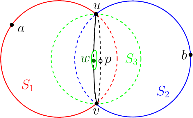
Figure 1: In three dimensions, three closed geodesic balls can all touch three points, $u,v,p$, on their boundary and yet no one of them is contained in the union of the other two.

An attempt to illustrate the problem is given in Figure 1, where $\tau=\{u,v,p\}$. Here, the sphere $S_{3}$ would be contained inside the spheres $S_{1}$ and $S_{2}$ if the metric were Euclidean, but any aberration in the metric may leave a part of $S_{3}$ exposed to the outside. This means that in principle another sample point $w$ could lie on $S_{3}$, while $S_{1}$ and $S_{2}$ remain empty. Thus there are three tetrahedra that share $\tau$ as a face.

The essential difference between dimension 2 and the higher dimensions can be observed by examining the topological intersection properties of spheres. Specifically, two $(m-1)$-spheres intersect transversely in an $(m-2)$-sphere. For a non-Euclidean metric, even if this property holds for sufficently small geodesic spheres, only in dimension two is the sphere of intersection of the Delaunay spheres of two adjacent $m$-simplices uniquely determined by the vertices of the shared $(m-1)$-simplex. See Figure 1.

2.4.4 The Voronoi diagram

We will occasionally make reference to the Voronoi diagram, which is a structure dual to the Delaunay complex. It offers an alternative way to interpret observations made with respect to the Delaunay complex.

The Voronoi cell associated with $p\in\mathsf{P}$ with respect to the metric $d:U\times U\to\mathbb{R}$ is given by

$$\mathcal{V}_{d}(p)=\{x\in U\,|\,d(x,p)\leq d(x,q)\text{ for all }q\in\mathsf{P}\}.$$

More generally, a Voronoi face is the intersection of a set of Voronoi cells: given $\{p_{0},\ldots,p_{k}\}\subset\mathsf{P}$, let $\sigma$ denote the corresponding abstract simplex. We define the associated Voronoi face as

$$\mathcal{V}_{d}(\sigma)=\bigcap_{i=0}^{k}\mathcal{V}_{d}(p_{i}).$$

It follows that $\sigma$ is a Delaunay simplex if and only if $\mathcal{V}_{d}(\sigma)\neq\emptyset$. In this case, every point in $\mathcal{V}_{d}(\sigma)$ is the centre of a Delaunay ball for $\sigma$. Thus every Voronoi face corresponds to a Delaunay simplex. The Voronoi cells give a decomposition of $U$, denoted $\operatorname{Vor}_{d}(\mathsf{P})$, called the Voronoi diagram. Our definition of the Delaunay complex of $\mathsf{P}$ corresponds to the nerve of the Voronoi diagram.

3 Equating Delaunay structures

We now turn to the task of triangulating $\mathcal{M}$, a smooth, compact $m$-manifold, without boundaries embedded in $\mathbb{R}^{N}$. In this section we demonstrate our main structural result, Theorem 3.5, which is stated at the end of Section 3.1. It says that the complex constructed by the algorithm we describe in Section 4 is in fact an intrinsic Delaunay triangulation of the manifold, which we introduce next.

3.1 Delaunay structures on manifolds

The restricted Delaunay complex is the Delaunay complex $\operatorname{Del}_{\mathbb{R}^{N}|_{\mathcal{M}}}(\mathcal{P})$ obtained when distances on the manifold are measured with the metric $d_{{\mathbb{R}^{N}|_{\mathcal{M}}}}$. This is the Euclidean metric of the ambient space, restricted to the submanifold $\mathcal{M}$. In other words, $d_{{\mathbb{R}^{N}|_{\mathcal{M}}}}(x,y)=d_{\mathbb{R}^{N}}(x,y)$. We use this notation to avoid ambiguities in conjunction with the local Euclidean metrics discussed below. The Delaunay complex $\operatorname{Del}_{\mathbb{R}^{N}|_{\mathcal{M}}}(\mathcal{P})$ is a substructure of $\operatorname{Del}_{\mathbb{R}^{N}}(\mathcal{P})$.

Alternatively, distances on the manifold may be measured with $d_{\mathcal{M}}$, the intrinsic metric of the manifold. This metric defines the distance between $x$ and $y$ as the infimum of the lengths of the paths on $\mathcal{M}$ which connect $x$ and $y$. Since the length of a path on $\mathcal{M}$ is defined as its length as a curve in $\mathbb{R}^{N}$, this metric is also induced from $d_{\mathbb{R}^{N}}$. The intrinsic Delaunay complex is the Delaunay structure $\operatorname{Del}_{\mathcal{M}}(\mathcal{P})$ associated with this metric.

Although neither of these metrics are Euclidean, the idea is that locally, in a small neighbourhood of any point, these metrics may be well approximated by $d_{\mathbb{R}^{m}}$. Then, if the sampling satisfies appropriate $\delta$-generic and $\epsilon$-dense criteria in these local Euclidean metrics, the global Delaunay complex in the metric of the manifold will coincide locally with a Euclidean Delaunay triangulation, and we can thus guarantee a manifold complex.

3.1.1 Local Euclidean metrics

A local coordinate chart at a point $p\in\mathcal{M}$, is a pair $(W,\phi_{p})$, where $W\subset\mathcal{M}$ is an open neighbourhood of $p$, and $\phi_{p}:W\to U=\phi_{p}(W)\subset\mathbb{R}^{m}$ is a homeomorphism onto its image, with $\phi_{p}(p)=0$. A local coordinate chart allows us to pull back the Euclidean metric to $W$. For all $x,y\in W$, the metric $d_{{\phi_{p}}}(x,y)=d_{\mathbb{R}^{m}}(\phi_{p}(x),\phi_{p}(y))$ is a a local Euclidean metric for $p$ on $W$. This metric depends upon the choice of $\phi_{p}$; there are different ways to impose a Euclidean metric on $W$.

It is convenient to take the reciprocal point of view, and work with a local parameterization at a point $p\in\mathcal{M}$. This is a pair $(U,\psi_{p})$, such that $U\subset\mathbb{R}^{m}$, and $(W,\psi_{p}^{-1})$ is a local coordinate chart for $p$, where $W=\psi_{p}(U)$. We can then use $\psi_{p}$ to pull back the metric of the manifold to $U$, and to simplify the notation we write $d_{\mathcal{M}}(x,y)$ for $x,y\in U$, where it is to be understood that this means $d_{\mathcal{M}}(\psi_{p}(x),\psi_{p}(y))$, and likewise for $d_{{\mathbb{R}^{N}|_{\mathcal{M}}}}(x,y)$. Indeed, once $W$ and $U$ have been coupled together by a homeomorphism, we can transfer the metrics between them and the distinction becomes only one of perspective; the standard metric $d_{\mathbb{R}^{m}}$ on $U$ is a local Euclidean metric for $p$.

We wish to generate a sample set $\mathcal{P}\subset\mathcal{M}$ that will allow us to exploit the stability results for Delaunay triangulations [BDG12]. We consider the stability of a Delaunay triangulation in a local Euclidean metric. The following definition is convenient when stating the stability results:

Definition 3.1 (Secure simplex).

A simplex $\sigma\in\operatorname{Del}(\mathsf{P})$ is secure if it is a $\delta$-protected $m$-simplex that is $\Upsilon_{0}$-thick and satisfies $R(\sigma)<\epsilon$ and $L(\sigma)\geq\mu_{0}\epsilon$.

We will make reference to the following result [BDG12, Theorem 4.17]:

Theorem 3.2 (Metric stability assuming thickness).

Suppose $\operatorname{conv}(\mathsf{P})\subseteq U\subset\mathbb{R}^{m}$ and the metric $d:U\times U\to\mathbb{R}$ is such that $\left|d(x,y)-d_{\mathbb{R}^{m}}(x,y)\right|\leq\rho$ for all $x,y\in U$. Suppose also that $\mathsf{P}_{J}\subseteq\mathsf{P}$ is such that every $m$-simplex $\sigma\in\operatorname{star}(\mathsf{P}_{J};\operatorname{Del}(\mathsf{P}))$ is secure and satisfies $d_{\mathbb{R}^{m}}(p,\partial{U})\geq 2\epsilon$ for every vertex $p\in\sigma$. If

$$\rho\leq\frac{\Upsilon_{0}\mu_{0}}{36}\delta,$$

then

$$\operatorname{star}(\mathsf{P}_{J};\operatorname{Del}_{d}(\mathsf{P}))=\operatorname{star}(\mathsf{P}_{J};\operatorname{Del}(\mathsf{P})).$$

In our context the point set $\mathsf{P}$ used in Theorem 3.2 will come from a larger point set $\mathcal{P}$, such that $\mathsf{P}=W\cap\mathcal{P}$. We will write $\mathsf{P}_{W}$ in order to emphasise this dependence on $W$. We want to ensure that

$$\operatorname{star}(\mathsf{P}_{J};\operatorname{Del}_{d}(\mathsf{P}_{W}))=\operatorname{star}(\mathsf{P}_{J};\operatorname{Del}_{d}(\mathcal{P})).$$ (3)

This requirement is attained by demanding that $\mathcal{P}$ satisfy a sampling radius of $\epsilon$ with respect to the metric $d_{\mathcal{M}}$. Since $d_{\mathbb{R}^{m}}(x,y)\leq d_{\mathcal{M}}(x,y)$ for all $x,y\in U\cong W$, by our particular choice of $\psi_{p}$, we will have that $\mathsf{P}_{W}$ is an $\epsilon$-sample set with respect to the metric $d_{\mathbb{R}^{m}}$. We ensure that $U$ is large enough so that $d_{\mathbb{R}^{m}}(p,\partial{U})\geq 4\epsilon$ for all $p\in\mathsf{P}_{J}$. It then follows that $R(\sigma)<\epsilon$ for any simplex $\sigma\in\operatorname{star}(\mathsf{P}_{J};\operatorname{Del}(\mathsf{P}_{W}))$, because $\mathsf{P}_{W}$ is an $\epsilon$-sample set [BDG12, Lemma 3.6], and thus $d_{\mathbb{R}^{m}}(q,\partial{U})\geq 2\epsilon$ for any $q\in\sigma$. It follows that $d_{\mathcal{M}}(q,\partial{U})\geq 2\epsilon$ as well, and thus the sampling radius on $\mathcal{P}$ ensures that Equation (3) is satisfied. For our purposes $\mathsf{P}_{J}$ will consist of a single point $p$, and the sampling radius $\epsilon$ is constrained by the requirement that $U$ be small enough that the metric distortion introduced by $\psi_{p}$ meets the requirements of Theorem 3.2.

3.1.2 The tangential Delaunay complex

The algorithm we describe in Section 4 is a variation of the algorithm described by Boissonnat and Ghosh [BG10]. This algorithm builds the tangential Delaunay complex, which we denote by $\operatorname{Del}_{T\mathcal{M}}(\mathcal{P})$. This is not a Delaunay complex as we have defined them, since it cannot be defined by the Delaunay empty ball criteria with respect to any single metric. However, it is a Delaunay-type structure, and as with $\operatorname{Del}_{\mathbb{R}^{N}|_{\mathcal{M}}}(\mathcal{P})$, the tangential Delaunay complex is a substructure of $\operatorname{Del}_{\mathbb{R}^{N}}(\mathcal{P})$. We will demonstrate sampling conditions which ensure that $\operatorname{Del}_{T\mathcal{M}}(\mathcal{P})=\operatorname{Del}_{\mathcal{M}}(\mathcal{P})=\operatorname{Del}_{\mathbb{R}^{N}|_{\mathcal{M}}}(\mathcal{P})$.

Definition 3.3 (Tangential Delaunay complex).

The tangential Delaunay complex for $\mathcal{P}\subset\mathcal{M}\subset\mathbb{R}^{N}$ is defined by the criterion that $\sigma\in\operatorname{Del}_{T\mathcal{M}}(\mathcal{P})$ if it has an empty circumscribing ball $B_{\mathbb{R}^{N}}(c,r)$ such that $c\in T_{p}{\mathcal{M}}$ for some vertex $p\in\sigma$.

We define some local complexes to facilitate discussions of the tangential Delaunay complex. For all $p\in\mathcal{P}$, let

$$K(p)=\{\sigma\;|\;\mathcal{V}_{\mathbb{R}^{N}}(\sigma)\cap T_{p}{\mathcal{M}}\neq\emptyset\},$$

and define

$$\operatorname{star}(p)=\operatorname{star}(p;K(p)).$$ (4)

Then the tangential Delaunay complex is the union of the complexes $\operatorname{star}(p)$ for all $p\in\mathcal{P}$.

Boissonnat et al. [BG11, Lemma 2.3] showed that $\mathcal{V}_{\mathbb{R}^{N}}(\mathcal{P})\cap T_{p}\mathcal{M}$ is equal to the $m$-dimensional weighted Voronoi diagram of $\mathcal{P}^{\prime}\subset T_{p}\mathcal{M}$, where $\mathcal{P}^{\prime}$ is the orthogonal projection of $\mathcal{P}$ onto $T_{p}\mathcal{M}$ and the squared weight of a point $p_{i}^{\prime}\in\mathcal{P}^{\prime}$ is $-\|p_{i}-p_{i}^{\prime}\|^{2}$. Therefore, $K(p)$ is isomorphic to a dual complex (the nerve) of the $k$-dimensional weighted Voronoi diagram of $\mathcal{P}^{\prime}$.

3.1.3 Power protection

The algorithm introduced in Section 4.2 will ensure that for every simplex $\sigma$ in the tangential Delaunay complex, and every vertex $p\in\sigma$, there is a Delaunay ball for $\sigma$ that is centred on $T_{p}{\mathcal{M}}$ and is protected in the following sense:

Definition 3.4 (Power protection).

A simplex $\sigma$ with Delaunay ball $B_{\mathbb{R}^{N}}(C,R)$ is $\check{\delta}^{2}$-power-protected if $d_{\mathbb{R}^{N}}(C,q)^{2}-R^{2}>\check{\delta}^{2}$ for all $q\in\mathcal{P}\setminus\sigma$.

Observe that, if $C\not\in\mathcal{M}$, the ball $B_{\mathbb{R}^{N}}(C,R)$ is not an object that can be described by the metric $d_{{\mathbb{R}^{N}|_{\mathcal{M}}}}$. In the context of the tangential Delaunay complex we use power-protection rather than the protection described in Section 2.4.1 because working with squared distances is convenient when we consider the Delaunay complex restricted to an affine subspace.

3.1.4 Main structural result

The rest of Section 3 is devoted to the proof of Theorem 3.5 below. It says that for the point set generated by our algorithm, the tangential Delaunay complex is isomorphic with the intrinsic Delaunay complex of $\mathcal{M}$. It then follows, from a previously published result [BG10, Theorem 5.1], that the intrinsic Delaunay complex is in fact homeormorphic to $\mathcal{M}$; it is an intrinsic Delaunay triangulation.

Thus we obtain a partial recovery of the kind of results attempted by Leibon and Letscher [LL00]. Our sampling conditions, and our algorithm (existence proof) rely on the embedding of $\mathcal{M}$ in $\mathbb{R}^{N}$; we leave purely intrinsic sampling conditions for future work.

Theorem 3.5 (Intrinsic Delaunay triangulation).

Suppose $\mathcal{P}\subset\mathcal{M}$ is $(\tilde{\mu}_{0}\epsilon)$-sparse with respect to $d_{\mathbb{R}^{N}}$, and every $m$-simplex $\tilde{\sigma}\in\operatorname{Del}_{T\mathcal{M}}(\mathcal{P})$ is $\tilde{\Upsilon}_{0}$-thick, and has, for every vertex $p\in\tilde{\sigma}$, a $\check{\delta}^{2}$-power-protected empty ball of radius less than $\epsilon$ centred on $T_{p}{\mathcal{M}}$, with $\check{\delta}\geq\delta_{0}\tilde{\mu}_{0}\epsilon$. If $\delta_{0}^{2}\tilde{\mu}_{0}^{2}\leq\frac{1}{7}$, and

$$\epsilon\leq\frac{\tilde{\Upsilon}_{0}^{2}\tilde{\mu}_{0}^{3}\delta_{0}^{2}\text{rch}(\mathcal{M})}{1.5\times 10^{6}},$$

then

$$\operatorname{Del}_{T\mathcal{M}}(\mathcal{P})=\operatorname{Del}_{\mathbb{R}^{N}|_{\mathcal{M}}}(\mathcal{P})=\operatorname{Del}_{\mathcal{M}}(\mathcal{P}),$$

and for $\epsilon$ sufficiently small, these will be homeomorphic to $\mathcal{M}$:

$$\left|\operatorname{Del}_{\mathcal{M}}(\mathcal{P})\right|\cong\mathcal{M}.$$

3.2 Choice of local Euclidean metric

A local parameterization at $p\in\mathcal{M}$ will be constructed with the aid of the orthogonal projection

$$\pi_{p}:\mathbb{R}^{N}\rightarrow T_{p}{\mathcal{M}},$$ (5)

restricted to $\mathcal{M}$. As shown in Lemma B.4, Niyogi et al. [NSW08, Lemma 5.4] demonstrated that if $r<\frac{\text{rch}(\mathcal{M})}{2}$, then $\pi_{p}$ is a diffeomorphism from $W=B_{\mathbb{R}^{N}|_{\mathcal{M}}}(p,r)$ onto its image $U\subset T_{p}{\mathcal{M}}$. We will identify $T_{p}{\mathcal{M}}$ with $\mathbb{R}^{m}$, and define the homeomorphism

$$\psi_{p}=\pi_{p}|_{W}^{-1}:U\longrightarrow W.$$ (6)

Using $\psi_{p}$ to pull back the metrics $d_{\mathcal{M}}$ and $d_{{\mathbb{R}^{N}|_{\mathcal{M}}}}$ to $\mathbb{R}^{m}$, we can view them as perturbations of $d_{\mathbb{R}^{m}}$. The magnitude of the perturbation is governed by the radius of the ball used to define $W$.

Definition 3.6.

We call a neighbourhood $W$ of $p\in\mathcal{M}$ admissible if $W\subseteq B_{\mathbb{R}^{N}|_{\mathcal{M}}}(p,r)$, with $r\leq\frac{\text{rch}(\mathcal{M})}{100}$.

In all that follows, any mention of a local Euclidean metric refers to the one defined by $\pi_{p}$ restricted to an admissible neighbourhood. The requirement $r\leq\frac{\text{rch}(\mathcal{M})}{100}$ is simply a convenient bound that yields a small integer constant in the perturbation bound of the following lemma, and does not constrain subsequent results. The bound could be relaxed to $r\leq\frac{\text{rch}(\mathcal{M})}{4}$ at the expense of a weaker bound on the perturbation.

Lemma 3.7 (Metric distortion).

Suppose $(U,\psi_{p})$ is a local parameterisation at $p\in W\subset\mathcal{M}$ with $W=\psi_{p}(U)$. If $W\subseteq B_{\mathbb{R}^{N}|_{\mathcal{M}}}(p,r)$, with $r\leq\frac{\text{rch}(\mathcal{M})}{100}$, then for all $x,y\in U$,

$$\left|d_{{\mathbb{R}^{N}|_{\mathcal{M}}}}(x,y)-d_{\mathbb{R}^{m}}(x,y)\right|\leq\left|d_{\mathcal{M}}(x,y)-d_{\mathbb{R}^{m}}(x,y)\right|\leq\frac{23r^{2}}{\text{rch}(\mathcal{M})}.$$

Proof.

Let $u,v\in W\subset B_{\mathbb{R}^{N}|_{\mathcal{M}}}(p,r)$, and let $\theta$ be the angle between the line segments $[u,v]$ and $[\pi_{p}(u),\pi_{p}(v)]$, $\theta_{1}$ the angle between $[u,v]$ and $T_{u}{\mathcal{M}}$, and $\theta_{2}$ the angle between $T_{p}{\mathcal{M}}$ and $T_{u}{\mathcal{M}}$. Thus $\theta\leq\theta_{1}+\theta_{2}$, and $d_{\mathbb{R}^{m}}(\pi_{p}(u),\pi_{p}(v))=d_{\mathbb{R}^{N}}(u,v){\cos\theta}$. Defining $\eta=\frac{r}{\text{rch}(\mathcal{M})}$, Lemma B.5 yields

$$d_{\mathcal{M}}(u,v)\leq d_{\mathbb{R}^{N}}(u,v)\left(1+4\eta\right),$$ (7)

and so

$$d_{\mathbb{R}^{m}}(\pi_{p}(u),\pi_{p}(v))\geq\frac{d_{\mathcal{M}}(u,v)\,\cos\theta}{1+4\eta}.$$

Using Lemma B.1, we find $\sin\theta_{1}\leq\eta$, and Lemma B.3, yields $\sin\theta_{2}\leq 6\eta$. Therefore, since $\sin\theta\leq\sin\theta_{1}+\sin\theta_{2}$, we have $\cos\theta=(1-\sin^{2}\theta)^{1/2}\geq 1-\sin\theta\geq 1-7\eta$ and we get

$$\begin{split}d_{\mathbb{R}^{m}}(\pi_{p}(u),\pi_{p}(v))&\geq{d_{\mathcal{M}}(u,v)}\left(\frac{1-7\eta}{1+4\eta}\right)\\ &\geq{d_{\mathcal{M}}(u,v)}\left(1-7\eta\right)(1-4\eta)\\ &\geq{d_{\mathcal{M}}(u,v)}(1-11\eta).\end{split}$$

Using Equation (7) we find $d_{\mathcal{M}}(u,v)\leq\frac{208r}{100}$, so $d_{\mathbb{R}^{m}}(\pi_{p}(u),\pi_{p}(v))\geq d_{\mathcal{M}}(u,v)-23\frac{r^{2}}{\text{rch}(\mathcal{M})}$, and the result follows since $d_{\mathcal{M}}(u,v)\geq d_{{\mathbb{R}^{N}|_{\mathcal{M}}}}(u,v)\geq d_{\mathbb{R}^{m}}(\pi_{p}(u),\pi_{p}(v))$.

Our sampling radius is constrained by the size of a Euclidean ball that can be contained in an admissible neighbourhood. The following lemma gives a convenient expression for this:

Lemma 3.8.

If $1<a\leq 10^{4}$ and $a\epsilon\leq\frac{\text{rch}(\mathcal{M})}{100}$, and $U=B_{\mathbb{R}^{m}}(p,(a-1)\epsilon)$, then $\psi_{p}(U)=W\subseteq B_{\mathbb{R}^{N}|_{\mathcal{M}}}(p,a\epsilon)$.

Proof.

Using Lemma B.1, we have that $B_{\mathbb{R}^{m}}(p,r)\subseteq\pi_{p}(B_{\mathbb{R}^{N}|_{\mathcal{M}}}(p,a\epsilon))$ if

$$\begin{split}r^{2}\leq a^{2}\epsilon^{2}-\left(\frac{a^{2}\epsilon^{2}}{2\text{rch}(\mathcal{M})}\right)^{2}&=a^{2}\epsilon^{2}\left(1-\left(\frac{a\epsilon}{2\text{rch}(\mathcal{M})}\right)^{2}\right)\\ &\leq a^{2}\epsilon^{2}\left(1-\left(\frac{1}{200}\right)^{2}\right).\end{split}$$

Thus we require $r\leq\sqrt{\frac{200^{2}-1}{200^{2}}}a\epsilon,$ which is satisfied by $r=(a-1)\epsilon$ if $a\leq 79999$.

Lemmas 3.7 and 3.8 lead to a sampling radius which allows us to employ Theorem 3.2, and so obtain an equivalence between Delaunay structures:

Proposition 3.9 (Equating Delaunay complexes).

Suppose $\mathcal{P}\subset\mathcal{M}$ is an $\epsilon$-sample set with respect to $d_{{\mathbb{R}^{N}|_{\mathcal{M}}}}$, and that for every $p\in\mathcal{P}$, in the local Euclidean metric on $W=B_{\mathbb{R}^{N}|_{\mathcal{M}}}(p,5\epsilon)$, every $m$-simplex in $\operatorname{star}(p;\operatorname{Del}(\mathsf{P}_{W}))$ is secure, where $\mathsf{P}_{W}=\mathcal{P}\cap W$, and $\delta=\nu_{0}\epsilon$. If

$$\epsilon\leq\frac{\Upsilon_{0}\mu_{0}\nu_{0}\text{rch}(\mathcal{M})}{20700}$$

then

$$\operatorname{star}(p;\operatorname{Del}(\mathsf{P}_{W}))=\operatorname{star}(p;\operatorname{Del}_{\mathbb{R}^{N}|_{\mathcal{M}}}(\mathsf{P}_{W}))=\operatorname{star}(p;\operatorname{Del}_{\mathcal{M}}(\mathsf{P}_{W})).$$ (8)

Thus

$$\operatorname{Del}_{\mathbb{R}^{N}|_{\mathcal{M}}}(\mathcal{P})=\operatorname{Del}_{\mathcal{M}}(\mathcal{P}),$$

and they are manifold complexes.

Proof.

As usual, let $U=\pi_{p}(W)$. Then by Lemma 3.8 $B_{\mathbb{R}^{m}}(p,4\epsilon)\subseteq U$, and thus $d_{\mathbb{R}^{m}}(q,\partial{U})\geq 2\epsilon$ for any vertex $q$ of a simplex in $\operatorname{star}(p;\operatorname{Del}(\mathsf{P}_{W}))$. Thus Lemma 3.7 allows us to apply Theorem 3.2 provided

$$\frac{23a^{2}\epsilon^{2}}{\text{rch}(\mathcal{M})}\leq\frac{\Upsilon_{0}\mu_{0}\nu_{0}\epsilon}{36},$$

when $a=5$, and we obtain the required bound on $\epsilon$. Thus the star of every vertex in $\operatorname{Del}_{\mathcal{M}}(\mathcal{P})$ is equal to the star of that point in the local Euclidean metric, and likewise for $\operatorname{Del}_{\mathbb{R}^{N}|_{\mathcal{M}}}(\mathcal{P})$. The claim follows since $\sigma\in\operatorname{Del}_{\mathcal{M}}(\mathcal{P})$ if and only if it is in the local Euclidean Delaunay triangulation of every one of its vertices, and likewise for the simplices in $\operatorname{Del}_{\mathbb{R}^{N}|_{\mathcal{M}}}(\mathcal{P})$.

3.3 The protected tangential complex

We obtain Theorem 3.5 by means of Theorem 3.2 via the observation that power protection of the ambient Delaunay balls translates into protection in the local Euclidean metrics. We must distinguish between the geometry of a simplex defined with respect to the Euclidean metric $d_{\mathbb{R}^{N}}$ of the ambient space, as opposed to a local Euclidean metric $d_{\mathbb{R}^{m}}$. In general, we use a tilda to indicate simplices in the ambient space, and their properties.

Lemma 3.10 (Protection under projection).

Suppose $\mathcal{P}\subset\mathcal{M}$ and that $\tilde{\sigma}\in\operatorname{Del}_{\mathbb{R}^{N}}(\mathcal{P})$ is an $\tilde{\Upsilon}_{0}$-thick $m$-simplex, with $L(\tilde{\sigma})\geq\tilde{\mu}_{0}\epsilon$ and $B_{\mathbb{R}^{N}}(C,R)$ is a $\check{\delta}^{2}$-power-protected empty ball for $\tilde{\sigma}$, with respect to the metric $d_{\mathbb{R}^{N}}$, where $\check{\delta}^{2}\geq\delta_{0}^{2}\tilde{\mu}_{0}^{2}\epsilon^{2}$. Suppose also that $C\in T_{p}{\mathcal{M}}$, for some vertex $p\in\tilde{\sigma}$.

If $R<\epsilon$, with

$$\epsilon\leq\frac{\tilde{\Upsilon}_{0}^{2}\tilde{\mu}_{0}^{3}\delta_{0}^{2}\text{rch}(\mathcal{M})}{512},$$ (9)

then $\sigma=\pi_{p}(\tilde{\sigma})$ has a $\delta$-protected Delaunay ball $B_{\mathbb{R}^{m}}(c,r)$ with respect to the local Euclidean metric $d_{\mathbb{R}^{m}}$ for $p$ on any admissible neighbourhood $W$ that contains $B_{\mathbb{R}^{N}|_{\mathcal{M}}}(p,3\epsilon)$, and $\delta=\nu_{0}\epsilon$, with

$$\nu_{0}=\frac{\delta_{0}^{2}\tilde{\mu}_{0}^{2}}{8}.$$ (10)

Proof.

We first find a bound for $d_{\mathbb{R}^{m}}(C,c)$ and $r$. Let $\tilde{\sigma}=[\tilde{p}_{0},\ldots,\tilde{p}_{m}]$, and $\sigma=[p_{0},\ldots,p_{m}]$ so that $\pi_{p}(\tilde{p}_{i})=p_{i}$, and $p=p_{0}=\tilde{p}_{0}$. We will first show that, near $C$, there is a circumcentre $c$ for $\sigma$ in the metric $d_{\mathbb{R}^{m}}$. For any $p_{i}\in\sigma$, $d_{\mathbb{R}^{N}}(p,p_{i})<2R$, and so by Lemma B.1 we have

$$d_{\mathbb{R}^{N}}(\tilde{p}_{i},p_{i})\leq\frac{2R^{2}}{\text{rch}(\mathcal{M})}<\frac{2\epsilon^{2}}{\text{rch}(\mathcal{M})}.$$

In order to apply Lemma 2.3 we require $\frac{2\epsilon^{2}}{\text{rch}(\mathcal{M})}\leq\frac{\tilde{\Upsilon}_{0}^{2}\tilde{\mu}_{0}\epsilon}{28}$, or

$$\epsilon\leq\frac{\tilde{\Upsilon}_{0}^{2}\tilde{\mu}_{0}\text{rch}(\mathcal{M})}{56},$$

which is satisfied by Equation (9). Since $\operatorname{aff}(\sigma)=T_{p}{\mathcal{M}}$, the circumcentre $c\in T_{p}{\mathcal{M}}$ is the closest point in $N(\sigma)$ to $C$, Lemma 2.3 yields

$$\left|R-r\right|\leq d_{\mathbb{R}^{m}}(C,c)=d_{\mathbb{R}^{N}}(C,c)<\frac{16\epsilon^{2}}{\tilde{\Upsilon}_{0}\tilde{\mu}_{0}\text{rch}(\mathcal{M})}.$$

Now we seek a lower bound on the protection of $B_{\mathbb{R}^{m}}(c,r)$. Suppose $\tilde{q}\in\mathcal{P}\setminus\tilde{\sigma}$. We wish to establish a lower bound on $d_{\mathbb{R}^{m}}(c,q)-r$, where $q=\pi_{p}(\tilde{q})$. We may assume that $d_{\mathbb{R}^{N}}(C,\tilde{q})<3\epsilon$, since otherwise $q$ will lie outside of our region of interest.

Let $z=\frac{(3\epsilon)^{2}}{2\text{rch}(\mathcal{M})}$ be the upper bound on $d_{\mathbb{R}^{N}}(\tilde{q},q)$ given by Lemma B.1. Then $d_{\mathbb{R}^{m}}(C,q)^{2}\geq d_{\mathbb{R}^{N}}(C,\tilde{q})^{2}-z^{2}>R^{2}+\check{\delta}^{2}-z^{2}$. Thus

$$d_{\mathbb{R}^{m}}(C,q)-R>\frac{\check{\delta}^{2}-z^{2}}{d_{\mathbb{R}^{m}}(C,q)+R}>\frac{\check{\delta}^{2}-z^{2}}{4\epsilon},$$

since $R<\epsilon$. Then $d_{\mathbb{R}^{m}}(c,q)-r\geq(d_{\mathbb{R}^{m}}(C,q)-d_{\mathbb{R}^{m}}(C,c))-(R+\left|R-r\right|)>\frac{\check{\delta}^{2}-z^{2}}{4\epsilon}-2d_{\mathbb{R}^{m}}(C,c)$. Putting this together, using $\check{\delta}^{2}\geq\delta_{0}^{2}\tilde{\mu}_{0}^{2}\epsilon^{2}$, we get

$$d_{\mathbb{R}^{m}}(c,q)-r>\left(\frac{1}{4}\delta_{0}^{2}\tilde{\mu}_{0}^{2}-\frac{81\epsilon^{2}}{16\text{rch}(\mathcal{M})^{2}}-\frac{32\epsilon}{\tilde{\Upsilon}_{0}\tilde{\mu}_{0}\text{rch}(\mathcal{M})}\right)\epsilon.$$

In order to simplify away the final term, we demand

$$\frac{32\epsilon}{\tilde{\Upsilon}_{0}\tilde{\mu}_{0}\text{rch}(\mathcal{M})}\leq\frac{1}{16}\delta_{0}^{2}\tilde{\mu}_{0}^{2},$$

which is satisfied by Equation (9). Under this constraint, the central term is also seen to be less than $\frac{1}{16}\delta_{0}^{2}\tilde{\mu}_{0}^{2}$, and we obtain

$$\delta\geq\frac{1}{8}\delta_{0}^{2}\tilde{\mu}_{0}^{2}\epsilon.$$

Proposition 3.9 requires a thickness $\Upsilon_{0}$ and shortest edge bound $\mu_{0}\epsilon$ for the simplex $\sigma\subset\mathbb{R}^{m}$, but Lemma 3.10 is expressed in terms of the corresponding quantities $\tilde{\Upsilon}_{0}$ and $\tilde{\mu}_{0}\epsilon$ for the corresponding simplex $\tilde{\sigma}\subset\mathbb{R}^{N}$.

Lemma 3.11 (Simplex distortion under projection).

Let $\tilde{\sigma}\in\operatorname{Del}_{\mathbb{R}^{N}}(\mathcal{P})$ be an $m$-simplex as described in Lemma 3.10, and let $\sigma=\pi_{p}(\tilde{\sigma})$ be its projection in the local Euclidean metric for $p$ on any admissible neighbourhood that contains $B_{\mathbb{R}^{N}|_{\mathcal{M}}}(p,2\epsilon)$, where $p$ is a vertex of $\tilde{\sigma}$. If $\epsilon$ satisfies Equation (9), and $\delta_{0}^{2}\tilde{\mu}_{0}^{2}\leq\frac{1}{7}$, then $L(\sigma)>\mu_{0}\epsilon$, where

$$\mu_{0}=\frac{20}{21}\tilde{\mu}_{0},$$

and $\Upsilon(\sigma)>\Upsilon_{0}$, where

$$\Upsilon_{0}=\frac{6}{49}\tilde{\Upsilon}_{0}.$$

Proof.

Since $\pi_{p}(B_{\mathbb{R}^{N}|_{\mathcal{M}}}(p,2\epsilon))\subseteq B_{\mathbb{R}^{m}}(p,2\epsilon)$, it is sufficient to apply the Metric distortion lemma 3.8 with $a=3$.

For the shortest edge length, we find

$$\begin{split}L(\sigma)&\geq L(\tilde{\sigma})-\frac{3^{2}\times 23\epsilon^{2}}{\text{rch}(\mathcal{M})}\\ &=\tilde{\mu}_{0}\left(1-\frac{207\tilde{\Upsilon}_{0}^{2}\delta_{0}^{2}\tilde{\mu}_{0}^{2}}{512}\right)\epsilon\\ &>\tilde{\mu}_{0}\left(1-\frac{\tilde{\Upsilon}_{0}^{2}\delta_{0}^{2}\tilde{\mu}_{0}^{2}}{3}\right)\epsilon\\ &>\frac{20}{21}\tilde{\mu}_{0}\epsilon.\end{split}$$

For the thickness bound, in order to apply Lemma 2.2, using $\tilde{\eta}=(1-\eta)$, we require

$$\frac{207\tilde{\Upsilon}_{0}^{2}\delta_{0}^{2}\tilde{\mu}_{0}^{3}}{512}\leq\frac{\tilde{\eta}\tilde{\Upsilon}_{0}^{2}\tilde{\mu}_{0}}{14},$$

which is satisfied if we choose

$$\tilde{\eta}>6\delta_{0}^{2}\tilde{\mu}_{0}^{2}.$$

Then Lemma 2.2 yields

$$\Upsilon(\sigma)\geq\frac{6}{7}\left(1-6\delta_{0}^{2}\tilde{\mu}_{0}^{2}\right)\Upsilon(\tilde{\sigma})>\frac{6}{49}\Upsilon(\tilde{\sigma}).$$

We can now express the sampling conditions in terms of the output parameters of the tangential complex algorithm, and this allows us to apply Proposition 3.9 and obtain our main structural result:

of Theorem 3.5.

We first translate the sampling requirements of Proposition 3.9 in terms of properties of simplices in the ambient metric $d_{\mathbb{R}^{N}}$. Using Lemma 3.11, together with Equation (10), the upper bound on the sampling radius demanded by Proposition 3.9 becomes

$$\epsilon\leq\frac{20\times 6\tilde{\Upsilon}_{0}\delta_{0}^{2}\tilde{\mu}_{0}^{3}\text{rch}(\mathcal{M})}{21\times 49\times 8\times 20700}.$$

We obtain the stated sampling radius bound after multiplying by $\tilde{\Upsilon}_{0}$ in order to ensure that the demand of Equation (9) is also met. Thus the stated sampling radius satisfies the requirements of both Lemma 3.10 and Proposition 3.9.

The fact that the structures are isomorphic follows from the fact that they are all locally isomorphic to the Delaunay triangulation in the local Euclidean metric. To see that $\operatorname{star}(p;\operatorname{Del}_{T\mathcal{M}}(\mathcal{P}))\cong\operatorname{star}(p;\operatorname{Del}(\mathsf{P}_{W}))$, observe that Lemma 3.10 implies that there is an injective simplicial map $\operatorname{star}(p;\operatorname{Del}_{T\mathcal{M}}(\mathcal{P}))\to\operatorname{star}(p;\operatorname{Del}(\mathsf{P}_{W}))$. The isomorphism is established by Lemma 2.9, once it is established that $\operatorname{star}(p;\operatorname{Del}_{T\mathcal{M}}(\mathcal{P}))$ is a triangulation at $p$. In fact $\operatorname{star}(p;\operatorname{Del}_{T\mathcal{M}}(\mathcal{P}))$ is isomorphic to the star of $p$ in a regular triangulation of the projected points $\mathsf{P}_{W}$; it is a weighted Delaunay triangulation [BG10], and with our choice of $W$, the point $p$ is an interior point in this triangulation [BG10, Lemma 2.7(1)]. Thus $\operatorname{star}(p;\operatorname{Del}_{T\mathcal{M}}(\mathcal{P}))$ is a triangulation at $p$, and it follows that

$$\operatorname{star}(p;\operatorname{Del}_{T\mathcal{M}}(\mathcal{P}))\cong\operatorname{star}(p;\operatorname{Del}(\mathsf{P}_{W})).$$

The equality of the Delaunay complexes now follows from Proposition 3.9, Equation (8).

The homeomorphism assertion follows from previous work [BG10, Theorem 5.1].

4 Algorithm

In this section we introduce a Delaunay refinement algorithm which, while constructing a tangential Delaunay complex, will transform the input sample set into one which meets the requirements of Theorem 3.5. In particular we wish to construct a tangential Delaunay complex in which every $m$-simplex $\sigma$ is $\tilde{\Upsilon}_{0}$-thick and for every $p\in\sigma$, there is a $\check{\delta}^{2}$-power-protected Delaunay ball for $\sigma$ centred on $T_{p}{\mathcal{M}}$. We demand $\check{\delta}\geq\delta_{0}\tilde{\mu}_{0}\epsilon$, where $\epsilon$ provides a strict upper bound on the radius of these Delaunay balls, and $\tilde{\mu}_{0}\epsilon$ provides a lower bound on the shortest edge length of any simplex in $\operatorname{Del}_{T\mathcal{M}}(\mathcal{P})$. The constants $\delta_{0}$ and $\tilde{\mu}_{0}$ are both positive and smaller than one.

The algorithm is in the same vein as that of Boissonnat and Ghosh [BG10], which is in turn an adaptation of the algorithm introduced by Li [Li03]. It is described in Section 4.2, after we introduce terminology and constructs which are used in the algorithm in Section 4.1.

4.1 Components of the algorithm

We now introduce the primary concepts that are used as building blocks of the algorithm.

4.1.1 Elementary weight functions

Elementary weight functions are a convenient device to facilitate the identification of simplices $\sigma$ that are not $\check{\delta}^{2}$-power-protected for $\check{\delta}=\delta_{0}L(\sigma)$.

In order to emphasise that we are considering a function defined only on the set of vertices of a simplex, we denote by $\mathring{\sigma}$ the set $\{p_{0},\,\dots,\,p_{k}\}$ of vertices of $\sigma=[p_{0}\,\dots\,p_{k}]$. We will call $\omega_{\sigma}:\mathring{\sigma}\rightarrow[0,\infty)$ an elementary weight function if it satisfies the following conditions:

1. There exists $p_{i}\in\mathring{\sigma}$ such that $\omega_{\sigma}(p_{i})\in[0,\,\delta_{0}L(\sigma)]$, and

2. for all $p_{j}\in\mathring{\sigma}\setminus p_{i}$, $\omega_{\sigma}(p_{j})=0$.

For a given $\sigma=[p_{0},\,\dots,\,p_{k}]$ and elementary weight function $\omega_{\sigma}$, we define $N(\sigma,\omega_{\sigma})$ as the set of solutions to the following system of $k$ equations:

$$\|x-p_{i}\|^{2}-\|x-p_{0}\|^{2}=\omega_{\sigma}(p_{i})^{2}-\omega_{\sigma}(p_{0})^{2}.$$

In direct analogy with the space $N(\sigma)$ of centres of $\sigma$, the set $N(\sigma,\omega_{\sigma})$ is an affine space of dimension $m-\dim\operatorname{aff}(\sigma)$ that is orthogonal to $\operatorname{aff}(\sigma)$. We denote by $C(\sigma,\omega_{\sigma})$ the unique point in $N(\sigma,\omega_{\sigma})\cap\operatorname{aff}(\sigma)$, and we define

$$R(\sigma,\omega_{\sigma})^{2}=\|p_{0}-C(\sigma,\omega_{\sigma})\|^{2}-\omega_{\sigma}(p_{0})^{2},$$

where the notation is chosen to emphasise the close relationship with the circumcentre $C(\sigma)$ and circumradius $R(\sigma)$. The following lemma exposes some properties of $R(\sigma,\omega_{\sigma})$ in this spirit:

Lemma 4.1.

For a given $\sigma=[p_{0},\dots,p_{k}]$, with $k\geq 1$, and elementary weight function $\omega_{\sigma}$, we have:

1. If $\sigma_{1}\leq\sigma$ then $\omega_{\sigma_{1}}=\omega_{\sigma}\mid_{\mathring{\sigma}_{1}}$ is an elementary weight function, and

   $$R(\sigma_{1},\omega_{\sigma_{1}})\leq R(\sigma,\omega_{\sigma}).$$

2. $\Delta(\sigma)\leq\frac{2}{1-\delta^{2}_{0}}\,R(\sigma,\omega_{\sigma})$.

3. If $\Upsilon(\sigma)>0$, then

   $$1-\eta\;\leq\;\frac{R(\sigma,\omega_{\sigma})}{R(\sigma)}\;\leq\;1+\eta,$$

   with $\eta=\frac{\delta^{2}_{0}}{\Upsilon(\sigma)}$.

Proof.

1. That $\omega_{\sigma_{1}}$ is an elementary weight function follows from the observation that $L(\sigma_{1})\geq L(\sigma)$. Since $N(\sigma,\omega_{\sigma})\subseteq N(\sigma_{1},\omega_{\sigma_{1}})$, the projection of $C(\sigma,\omega_{\sigma})$ into $\operatorname{aff}(\sigma_{1})$ is $C(\sigma_{1},\omega_{\sigma_{1}})$. The result then follows from the Pythagorean theorem.

2. Let $e=[p_{0},p_{1}]$ be the longest edge of $\sigma$, and let $c$ denote the projection of $C(\sigma,\omega_{\sigma})$ onto $\operatorname{aff}(e)$. Without loss of generality we assume that $\omega(p_{0})=0$.

We have

$$\begin{split}\left\|p_{0}-c\right\|^{2}&=\left\|p_{1}-c\right\|^{2}-\omega_{\sigma}(p_{1})^{2}\\ &=\left\|(p_{1}-p_{0})-(c-p_{0})\right\|^{2}-\omega_{\sigma}(p_{1})^{2}\\ &=\Delta(\sigma)^{2}-2(p_{1}-p_{0})\cdot(c-p_{0})+\left\|p_{0}-c\right\|^{2}-\omega_{\sigma}(p_{1})^{2}.\\ \end{split}$$

Since $p_{0}$, $p_{1}$, and $c$ are colinear, we have $2(p_{1}-p_{0})\cdot(c-p_{0})=2\Delta(\sigma)\left\|p_{0}-c\right\|$, and using the fact that $\omega_{\sigma}(p_{1})\leq\delta_{0}L(\sigma)$, we get

$$\begin{split}\|p_{0}-c\|&=\frac{\Delta(\sigma)}{2}\left(1-\frac{\omega_{\sigma}(p_{1})^{2}}{\Delta(\sigma)^{2}}\right)\\ &\geq\frac{(1-\delta^{2}_{0})\Delta(\sigma)}{2}.\end{split}$$

The result follows from the fact that $R(\sigma,\omega_{\sigma})\geq\|p_{0}-c\|$.

3. Using the fact that $\omega_{\sigma}(p)=0$ for all vertices $p\in\mathring{\sigma}$, except at most one, we get $p_{i}\in\partial B_{\mathbb{R}^{k}}(C(\sigma,\omega_{\sigma}),R(\sigma,\omega_{\sigma}))$ for all $p_{i}\in\mathring{\sigma}$ except at most one.

Let $\eta=\|C(\sigma,\omega_{\sigma})-C(\sigma)\|$, and assume, without loss of generality, that the vertex $p_{0}\in\partial B(C(\sigma,\omega_{\sigma}),R(\sigma,\omega_{\sigma}))$. Therefore,

$$\|C(\sigma)-p_{0}\|-\eta\;\;\leq \|C(\sigma,\omega_{\sigma})-p_{0}\| \leq\;\;\|C(\sigma)-p_{0}\|+\eta$$

$$R(\sigma)+\eta\;\;\leq R(\sigma,\omega_{\sigma}) \leq\;\;R(\sigma)+\eta.$$ (11)

Since the point in $N(\sigma)$ that is closest to $C(\sigma,\omega_{\sigma})$ is $C(\sigma)$, and $\Upsilon(\sigma)>0$, we obtain the following bound using Lemma 4.1 from [BDG12]:

$$\eta \leq \frac{\delta_{0}^{2}L(\sigma)^{2}}{2\Upsilon(\sigma)\Delta(\sigma)}$$ (12)

$$\leq \frac{\delta^{2}_{0}}{\Upsilon(\sigma)}R(\sigma),~{}~{}~{}~{}\mbox{since $L(\sigma)\leq\Delta(\sigma)\leq 2R(\sigma)$.}$$

The result now follows from Eq. (4.1.1) and (12).

If $\sigma={p}*{\sigma_{p}}$, and $\omega_{\sigma}$ is an elementary weight function that vanishes on $\mathring{\sigma_{p}}$, then $N(\sigma,\omega_{\sigma})\subseteq N(\sigma_{p})$, but no point in $N(\sigma,\omega_{\sigma})$ can be the centre of a $\check{\delta}^{2}$-power-protected Delaunay ball for $\sigma_{p}$ for any $\check{\delta}\geq\delta_{0}L(\sigma)$. In other words, $\sigma$ and $\omega_{\sigma}$ define a quasi-cospherical configuration that is an obstruction to the power protection of $\sigma_{p}$ at all points in $N(\sigma,\omega_{\sigma})$.

4.1.2 Quasicospherical configurations

We now define the family of simplices that our algorithm must eliminate in order to ensure that the final point set has the desired protection properties.

Recalling the definition (4) of $\operatorname{star}(p)$, we have the following [BG10, Lemma 2.7 (1)]:

Lemma 4.2.

Let $\mathcal{P}\subset\mathcal{M}$ satisfy a sampling radius of $\epsilon$ with respect to $d_{\mathbb{R}^{N}}$ such that $\epsilon\leq{\text{rch}(\mathcal{M})}/{16}$. Then for all $x\in\mathcal{V}_{\mathbb{R}^{N}}(p)\cap T_{p}\mathcal{M}$, we have $\|p-x\|\leq 4\epsilon$. In particular, for all $p\in\mathcal{P}$, and every $m$-simplex $\sigma\in\operatorname{star}(p)$, we have $R_{p}(\sigma)\leq 4\epsilon$.

Since by Lemma 4.2, the Voronoi cell of $p$ restricted to $T_{p}{\mathcal{M}}$ is bounded, we get:

Lemma 4.3.

If $\epsilon\leq\frac{\text{rch}(\mathcal{M})}{16}$, then the combinatorial dimension of the maximal simplices in $\operatorname{star}(p)$ is at least $m$.

We will always assume that $\mathcal{P}$ satisfies a sampling radius of $\epsilon\leq\frac{\text{rch}(\mathcal{M})}{16}$. If $\sigma$ is a maximal simplex in $\operatorname{star}(p)$, then $\mathcal{V}_{\mathbb{R}^{N}}(\sigma)$ intersects $T_{p}{\mathcal{M}}$ at a single point. Indeed, since $\mathcal{V}_{\mathbb{R}^{N}}(\sigma)\subset\mathcal{V}_{\mathbb{R}^{N}}(p)$, by Lemma 4.2 the convex set $\mathcal{V}_{\mathbb{R}^{N}}(\sigma)\cap T_{p}{\mathcal{M}}$ is bounded, and if it had a nonempty interior, then $\sigma$ would not be maximal. Let $\sigma$ be a maximal simplex in $\operatorname{star}(p)$. Then, for all $\sigma^{m}\leq\sigma$, the unique point in $\mathcal{V}_{\mathbb{R}^{N}}(\sigma)\,\cap\,T_{p}\mathcal{M}\,.$ will be denoted by $c_{p}(\sigma^{m})$. We denote the radius of the circumscribing ball centred at $c_{p}(\sigma^{m})$ by $R_{p}(\sigma^{m})$, i.e., $R_{p}(\sigma^{m})=\left\|p-c_{p}(\sigma^{m})\right\|$.

In our algorithm we will use the following complex, whose definition employs a particular elementary weight function:

$$\operatorname{cosph}^{\delta_{0}}(p) =\Bigg{\{}~{}\sigma^{m+1}=p_{m+1}*\sigma^{m}\;\big{|}\;\sigma^{m}\in\operatorname{star}(p),\,R_{p}(\sigma^{m})<\epsilon,$$

$$\quad\quad~{}\sigma^{m}~{}\mbox{is $\Gamma_{0}$-good, and }\exists\,\omega_{\sigma^{m+1}}\mbox{ with }\omega_{\sigma^{m+1}}|_{\mathring{\sigma}^{m}}=0$$

$$\quad\quad~{}\mbox{and}~{}c_{p}(\sigma^{m})\in N(\sigma^{m+1},\omega_{\sigma^{m+1}})\Bigg{\}}.$$ (13)

The $(m+1)$-dimensional simplices in $\operatorname{cosph}^{\delta_{0}}(p)$ are analogous to inconsistent configurations defined in [BG10, BG11].

Unless otherwise stated, whenever $\sigma^{m+1}=p_{m+1}*\sigma^{m}\in\operatorname{cosph}^{\delta_{0}}(p)$, with $\sigma^{m}\in\operatorname{star}(p)$, the mention of $\omega_{\sigma^{m+1}}$ will refer to the elementary weight function identified in Equation (4.1.2). In particular,

$$\omega_{\sigma^{m+1}}(p_{i})=0\text{ for all }p_{i}\in\mathring{\sigma}^{m+1}\setminus p_{m+1},$$

and

$$\omega_{\sigma^{m+1}}(p_{m+1})\in[0,\delta_{0}L(\sigma^{m+1})]$$

satisfies

$$\|c_{p}(\sigma^{m})-p\|^{2}=\|c_{p}(\sigma^{m})-p_{m+1}\|^{2}-\omega_{\sigma^{m+1}}(p_{m+1})^{2}.$$

We will exploit the following observations:

Lemma 4.4.

If $\sigma^{m+1}={p_{m+1}}*{\sigma^{m}}\in\operatorname{cosph}^{\delta_{0}}(p)$ with $\sigma^{m}\in\operatorname{star}(p)$, then

$$R(\sigma^{m+1},\omega_{\sigma^{m+1}})\leq R_{p}(\sigma^{m})$$

and

$$\Delta(\sigma^{m+1})\leq\frac{2}{1-\delta^{2}_{0}}R_{p}(\sigma^{m})$$

Proof.

Since $c_{p}(\sigma^{m})\in N(\sigma^{m+1},\omega_{\sigma^{m+1}})$, it follows that $C(\sigma^{m+1},\omega_{\sigma^{m+1}})$ is the projection of $c_{p}(\sigma^{m})$ into $\operatorname{aff}(\sigma^{m+1})$, and therefore $R_{p}(\sigma^{m})\geq R(\sigma^{m+1},\omega_{\sigma^{m+1}})$. The bound on $\Delta(\sigma^{m+1})$ now follows directly from Lemma 4.1.

Boissonnat et al. [BG11], using Lemma 4.2, showed that we can compute $\operatorname{star}(p)$ by computing a weighted Delaunay triangulation on $T_{p}{\mathcal{M}}$ of the points obtained by projecting $\mathcal{P}$ onto $T_{p}\mathcal{M}$. Once $\operatorname{star}(p)$ has been computed, we can compute $\operatorname{cosph}^{\delta_{0}}(p)$ by a simple distance computation.

The importance of $\operatorname{cosph}^{\delta_{0}}(p)$ lies in the observation that if an $m$-simplex $\sigma^{m}\in\operatorname{star}(p)$ is not sufficiently power-protected, then there will be a simplex in $\operatorname{cosph}^{\delta_{0}}(p)$ that is a witness to this. It is a direct consequence of the definitions, but we state it explicitly for reference:

Lemma 4.5.

If $\mathcal{P}$ is $\tilde{\mu}_{0}\epsilon$-sparse, and $\operatorname{cosph}^{\delta_{0}}(p)=\emptyset$, then every $\sigma^{m}\in\operatorname{star}(p)$ is $\delta_{0}^{2}\tilde{\mu}_{0}^{2}\epsilon^{2}$-power protected on $T_{p}\mathcal{M}$.

4.1.3 Unfit configurations and the picking region

The refinement algorithm, at each step, kills an unfit configuration by inserting a new point $x=\psi_{p}(x^{\prime})$ where $x^{\prime}$ belongs to the so-called picking region of the unfit configuration, and $\psi_{p}$ is the inverse projection defined in Equation (6). We use the term unfit configuration to distinguish the elements under consideration from other simplices. An unfit configuration $\phi$ may be one of two types:

Big configuration:

An $m$-simplex $\phi=\sigma^{m}$ in $\operatorname{star}(p)$ is a big configuration if $R_{p}(\sigma^{m})\geq\epsilon$.

Bad configuration:

A simplex $\phi$ is a bad configuration if it is $\Gamma_{0}$-bad and it is either an $m$-simplex $\phi=\sigma^{m}\in\operatorname{star}(p)$ that is not a big configuration, or it is an $(m+1)$-simplex $\phi=\sigma^{m+1}\in\operatorname{cosph}^{\delta_{0}}(p)$.

We will show in Section 5.2, Lemma 5.13, that in fact every $(m+1)$-simplex in $\operatorname{cosph}^{\delta_{0}}(p)$ is a bad configuration.

The size of the picking region is governed by a positive parameter $\alpha<1$ called the picking ratio.

Definition 4.6 (Picking region).

The picking region of a bad configuration, $\sigma^{m}\in\operatorname{star}(p)$ or $p_{m+1}*\sigma^{m}\in\operatorname{cosph}^{\delta_{0}}(p)$ with $\sigma^{m}\in\operatorname{star}(p)$, denoted by $P(\sigma^{m},p)$ and $P(\sigma^{m+1},p)$ respectively, is defined to be the $m$-dimensional ball

$$B_{\mathbb{R}^{N}}(c_{p}(\sigma^{m}),\alpha R_{p}(\sigma^{m}))\cap~{}T_{p}{\mathcal{M}}.$$

We choose a point in the picking region so as to minimize the introduction of new unfit configurations. We are able to avoid creating new bad configurations provided that the radius of the potential configuration is not too large. To this end, we introduce the parameter $\beta>1$.

Definition 4.7 (Hitting sets and good points).

Let $\phi=\sigma^{m}\in\operatorname{star}(p)$ or $\phi=q*\sigma^{m}\in\operatorname{cosph}^{\delta_{0}}(p)$ with $\sigma^{m}\in\operatorname{star}(p)$, and $x=\psi_{p}(y)$ where $y\in P(\phi,p)$. A set $\sigma\subset\mathcal{P}$ of size $k$, with $k\leq m+1$, is called a hitting set of $x$ if

a. $\tau=x*\sigma$ is a $k$-dimensional $\Gamma_{0}$-flake

and there exists an elementary weight function $\omega_{\tau}$ satisfying the following condition:

b. $R(\tau,\omega_{\tau})<\beta R_{p}(\sigma^{m})$

The elementary weight function $\omega_{\tau}$ is called a hitting map, and we sometimes say $\sigma$ hits $x$.

A point $x=\psi_{p}(y)$, where $y\in P(\phi,p)$, is said to be a good point if it is not hit by any set $\sigma\subset\mathcal{P}$ with $|\sigma|\leq m+1$.

A simplex $\sigma$ which defines a hitting set of $x$, is necessarily $\Gamma_{0}$-good. This follows from the requirement that ${x}*{\sigma}$ be a $\Gamma_{0}$-flake.

4.2 The refinement algorithm

In this section, we show that we can refine an $\epsilon$-net of $\mathcal{M}$ so that the simplices of the Delaunay tangential complex of the refined sample $\operatorname{Del}_{T\mathcal{M}}(\mathcal{P})$ are power-protected. An $\epsilon$-net is a point sample ${\mathcal{P}}\subset\mathcal{M}$ that is an $\epsilon$-sparse $\epsilon$-sample set of $\mathcal{M}$ for the metric $d_{\mathbb{R}^{N}}$. One can obtain an $\epsilon$-net by using a farthest point strategy to select a subset of a sufficiently dense sample set. We will assume that we know the dimension $m$ of the submanifold $\mathcal{M}$ and the tangent space $T_{p}\mathcal{M}$ at any point $p$ in $\mathcal{M}$.

The algorithm takes as input $\mathcal{P}_{0}$, an $\epsilon$-net of $\mathcal{M}$, and the positive input parameters $\epsilon$, $\Gamma_{0}$, $\alpha<\frac{1}{2}$, $\beta>1$ and $\delta_{0}<\frac{1}{4}$. The algorithm refines the input point sample such that:

1. The output sample $\mathcal{P}\supseteq\mathcal{P}_{0}$ is an $\tilde{\mu}_{0}\epsilon$-sparse $\epsilon$-sample set of $\mathcal{M}$ with respect to $d_{\mathbb{R}^{N}}$, where $\mu_{0}=\frac{1}{9}$.

2. For all $p\in\mathcal{P}$, every $m$-simplex $\sigma^{m}\in\operatorname{star}(p;\operatorname{Del}_{T\mathcal{M}}(\mathcal{P}))$, $\sigma^{m}$ is $\Gamma_{0}$-good and $\delta_{0}^{2}\tilde{\mu}_{0}^{2}\epsilon^{2}$-power protected on $T_{p}{\mathcal{M}}$.

Algorithm 1 Refinement algorithm

  Input     $\epsilon$-net ${\mathcal{P}_{0}}$ of $\mathcal{M}$, and input parameters $\Gamma_{0}$, $\alpha$ and $\delta_{0}$;

  Initalize  $\mathcal{P}\leftarrow\mathcal{P}_{0}$, and calculate $\operatorname{Del}_{T\mathcal{M}}(\mathcal{P})$;

  Rule (1) Big configuration ($\epsilon$-big radius):            if $\exists\;p\in\mathcal{P}$ such that $\exists\;\sigma^{m}\in\operatorname{star}(p)$ with $R_{p}(\sigma^{m})\geq\epsilon$,            then Insert$(\psi_{p}(c_{p}(\sigma^{m})))$;

  Rule (2) Bad configuration ($\Gamma_{0}$-bad):            if $\exists\;p\in\mathcal{P}$ and $\exists\;\sigma^{m}\in\operatorname{star}(p)$ s.t. $\sigma^{m}$ is $\Gamma_{0}$-bad,             then Insert$({\rm Pick\_valid}(\sigma^{m},p))$;            if $\exists\;p\in\mathcal{P}$ and $\exists\;\sigma^{m+1}\in\operatorname{cosph}^{\delta_{0}}(p)$ s.t. $\sigma^{m+1}$ is $\Gamma_{0}$-bad,             then Insert$({\rm Pick\_valid}(\sigma^{m+1},p))$;

  Output  $\operatorname{Del}_{T\mathcal{M}}(\mathcal{P})=\cup_{p\in\mathcal{P}}\;\operatorname{star}(p)$;

The algorithm, described in Algorithm 1, applies two rules with a priority order: Rule (2) is applied only if Rule (1) cannot be applied. The algorithm ends when no rule applies any more. Each rule inserts a new point to kill an unfit configuration: either a big configuration or a bad configuration.

A crucial procedure, that selects the location of the point to be inserted, is Pick_valid, given in Algorithm 2. Pick_valid$(\phi,p)$ returns a good point $\psi_{p}(y)$ where $y\in P(\phi,p)$.

Algorithm 2 Pick_valid$(\sigma,p)$

  // Assume that $\sigma$ is either equal to $\sigma^{m}\in\operatorname{star}(p)$

  // or $\sigma^{m+1}=p_{m+1}*\sigma^{m}\in\operatorname{cosph}^{\delta_{0}}(p)$ with $\sigma^{m}\in\operatorname{star}(p)$

  Step 1. Pick randomly $y\in P(\sigma^{m},p)$ (or $P(\sigma^{m+1},p)$);

  // Recall that $\psi_{p}$ projects points from $T_{p}\mathcal{M}$ onto $\mathcal{M}$ along $N_{p}\mathcal{M}$

  Step 2. $x\leftarrow\psi_{p}(y)$;

  Step 3. Avoid hitting sets:            // $|\tilde{\sigma}|$ denotes the cardinality of $\tilde{\sigma}$           if $\exists\;\tilde{\sigma}\subset\mathcal{P}$, with $|\tilde{\sigma}|\leq m+1$, which is a hitting set of $x$,           then discard $x$, and go back to Step 1;

  Step 4. Return $x$;

The refinement algorithm will also use the procedure Insert$(p)$, given in Algorithm 3.

Algorithm 3 Insert$(p)$

  Step 1. Add $p$ to $\mathcal{P}$;

  Step 2. Compute $\operatorname{star}(p)$ and $\operatorname{cosph}^{\delta_{0}}(p)$;

  Step 3. For all $x\in\mathcal{P}\setminus\{p\}$, update $\operatorname{star}(x)$ and $\operatorname{cosph}^{\delta_{0}}(x)$;

5 Analysis of the algorithm

We now turn to the demonstration of the correctness of Algorithm 1. In Section 5.1 we show that the algorithm must terminate, and in Section 5.2 we show that the output of the algorithm meets the requirements of Theorem 3.5. In order to complete the demonstrations we impose a number of requirements on the input parameters, listed as Hypotheses $\mathcal{H}0$ to $\mathcal{H}5$ below.

Recall that our input parameters are the following positive numbers: $\epsilon$, which is the sampling radius and sparsity bound satisfied by $\mathcal{P}_{0}$, the input $\epsilon$-net sample set; $\delta_{0}$, which is used to describe the amount of power-protection enjoyed by the $m$-simplices in the final complex; $\Gamma_{0}$, which is used to quantify the quality of the output simplices; $\beta$, which is used to describe an upper bound on the radius of the bad configurations that we will avoid; and $\alpha$, which governs the relative size of the picking region.

It is often convenient to represent the sampling radius by a dimension-free parameter that has the reach of the manifold factored out. We define

$$\tilde{\epsilon}=\frac{\epsilon}{\text{rch}(\mathcal{M})}.$$

The volume of the $m$-dimensional Euclidean unit-ball is denoted $V_{m}$. In order to state the hypotheses on the input parameters, we use some additional symbols:

$$\tilde{\epsilon}_{0} =\frac{1}{2^{4}(2^{4}+1)^{2}},$$

$$B =4+2(1+2^{7}3^{2}\beta^{2})^{2},$$

$$\beta^{\prime} =\frac{\beta}{1-2^{4}\tilde{\epsilon}_{0}},$$

as well as $\xi$, $E$, and $D$. The term $\xi$ is introduced in Lemma 5.5, and depends on $m$ and $\text{rch}(\mathcal{M})$, and the term $E$, defined in Equation (17), depends on $\xi$ and $\beta$. The symbol $D$ is introduced in Lemma 5.8, where it is said to depend on $m$ and $\beta$.

In order to guarantee termination, we demand the following hypotheses on the input parameters:

${\mathcal{H}0}$.

$\alpha<1/2$

${\mathcal{H}1}$.

$\beta\geq\frac{2}{(1-\delta^{2}_{0})(1-\alpha-4.5\,\tilde{\epsilon}_{0})}$

${\mathcal{H}2}$.

$\Gamma_{0}<\min\left\{\frac{V_{m}\alpha^{m}}{E^{m+1}\beta^{m}D},\frac{1}{B+1}\right\}$

${\mathcal{H}3}$.

$\delta^{2}_{0}\leq\Gamma^{m+1}_{0}$

${\mathcal{H}4}$.

$\tilde{\epsilon}\leq\min\left\{\frac{\xi}{2(\beta+\beta^{\prime})\text{rch}(\mathcal{M})},\,\frac{\Gamma^{m+1}_{0}}{8\beta}\right\}$

To meet the quality requirements of Theorem 3.5 we demand an additional constraint on the sampling radius:

${\mathcal{H}5.}$

$\tilde{\epsilon}\leq\frac{\delta^{2}_{0}\Gamma^{2m}_{0}}{1.1\times 10^{9}}$

The make use of the following observation:

Lemma 5.1.

From hypotheses ${\mathcal{H}0}$ to ${\mathcal{H}4}$ we have $\tilde{\epsilon}<\tilde{\epsilon}_{0}$ and $\delta^{2}_{0}<2^{4}\,\tilde{\epsilon}_{0}$, and

$$\frac{(1-\delta^{2}_{0})(1-\alpha-4.5\tilde{\epsilon}_{0})\epsilon}{4}>\frac{\epsilon}{9}\stackrel{{\scriptstyle{\rm def}}}{{=}}\tilde{\mu}_{0}\epsilon.$$ (14)

Proof.

From ${\mathcal{H}}1$ we have $\beta>2$ and using the fact that $B>\beta^{4}$ and ${\mathcal{H}}2$ we have $\Gamma_{0}<\frac{1}{2^{4}+1}$. And using the fact, from ${\mathcal{H}4}$, that

$$\tilde{\epsilon}\leq\frac{\Gamma_{0}^{m+1}}{8\beta}\leq\frac{\Gamma_{0}^{2}}{8\beta}<\frac{1}{2^{4}(2^{4}+1)^{2}}=\tilde{\epsilon}_{0}.$$

Similarly the bound on $\delta^{2}_{0}$ follows from ${\mathcal{H}}3$.

Inequality (14) follows from $\mathcal{H}0$ and the definition of $\tilde{\epsilon}_{0}$.

From Equation (14) we can see that we require $\beta\geq 4.5$. Given $\alpha$ satisfying $\mathcal{H}0$, and a valid choice for $\beta$, the hypotheses $\mathcal{H}2$ to $\mathcal{H}4$ sequentially yield upper bounds on the parameters $\Gamma_{0}$, $\delta_{0}$, and $\tilde{\epsilon}$; we are able to choose parameters that satisfy all of the hypotheses.

The main result of this section can now be summarised:

Theorem 5.2 (Algorithm guarantee).

If the input parameters satisfy hypotheses $\mathcal{H}0$ to $\mathcal{H}5$, then Algorithm 1 terminates after producing an intrinsic Delaunay complex $\operatorname{Del}_{\mathcal{M}}(\mathcal{P})$ that triangulates $\mathcal{M}$.

5.1 Termination of the algorithm

This subsection is devoted to the proof of the following theorem:

Theorem 5.3 (Algorithm termination).

Under hypotheses $\mathcal{H}0$ to $\mathcal{H}4$, the application of Rule $(1)$ or Rule $(2)$ on a big or a bad configuration $\phi$ always leaves the interpoint distance greater than

$$\tilde{\mu}_{0}\epsilon=\frac{\epsilon}{9},$$

and if $\phi$ is a bad configuration then there exists $x\in P(\phi,p)$ such that $\psi_{p}(x)$ is a good point. Since $\mathcal{M}$ is a compact manifold this implies that the refinement algorithm terminates and returns a point sample $\mathcal{P}$ which is an $\tilde{\mu}_{0}\epsilon$-sparse $\epsilon$-sample of the manifold $\mathcal{M}$.

We will prove that at every step the algorithm maintains the following two invariants:

Sparsity:

Whenever a refinement rule inserts a new point $x=\psi_{p}(y)$, the distance between $x$ and the existing point set $\mathcal{P}$ is greater than $\tilde{\mu}_{0}\epsilon$.

Good points:

For a bad configuration $\phi$ refined by Rule (2), there exists a set of positive volume $G\subseteq P(\phi,p)$ such that if $x\in G$, then $\psi_{p}(x)$ is a good point.

The Termination Theorem 5.3 is a direct consequence of these two algorithmic invariants. We first prove the sparsity invariant in Section 5.1.1, using an induction argument that relies on the fact that the algorithm only inserts good points. The existence of good points is then established in Section 5.1.2, using the sparsity invariant and a volumetric argument. Termination must follow since $\mathcal{M}$ is compact and therefore can only support a finite number of sample points satisfying a minimum interpoint distance.

5.1.1 The sparsity invariant

The proof of the sparsity invariant employs the following observation, which serves to bound the distance between a point inserted by Rule (2) and the existing point set:

Lemma 5.4.

Assume Hypotheses ${\mathcal{H}0}$ to ${\mathcal{H}4}$. Let $\phi=\sigma^{m}\in\operatorname{star}(p)$ or $\phi=p_{m+1}*\sigma^{m}\in\operatorname{cosph}^{\delta_{0}}(p)$ be a bad configuration being refined by Rule (2). Then for all $x\in P(\phi,p)$ we have

$$d_{\mathbb{R}^{N}}(c_{p}(\sigma^{m}),\psi_{p}(x))<(\alpha+4.5\tilde{\epsilon}_{0})R_{p}(\sigma^{m})$$

and

$$d_{\mathbb{R}^{N}}(\psi_{p}(x),\mathcal{P})>(1-\alpha-4.5\tilde{\epsilon}_{0})R_{p}(\sigma^{m})>\frac{R_{p}(\sigma^{m})}{3}.$$

Proof.

Using the facts that $\alpha<\frac{1}{2}$, and $\tilde{\epsilon}<\tilde{\epsilon}_{0}$, and $R_{p}(\sigma^{m})<\epsilon$, we have that for all $x\in P(\phi,p)$

$$\|p-x\|<(1+\alpha)R_{p}(\sigma^{m})<\frac{3\epsilon}{2}<\frac{3\,\tilde{\epsilon}_{0}}{2}<\frac{1}{4},$$

and so we may apply Lemma B.2 to get

$$\|x-\psi_{p}(x)\|\leq\frac{2\|p-x\|^{2}}{\text{rch}(\mathcal{M})}\leq\frac{2(1+\alpha)^{2}R_{p}(\sigma^{m})^{2}}{\text{rch}(\mathcal{M})}\leq 4.5\,\tilde{\epsilon}_{0}R_{p}(\sigma^{m}),$$

and

$$\|c_{p}(\sigma^{m})-\psi_{p}(x)\| \leq \|c_{p}(\sigma^{m})-x\|+\|x-\psi_{p}(x)\|$$ (15)

$$\leq \left(\alpha+4.5\,\tilde{\epsilon}_{0}\right)\,R_{p}(\sigma^{m}).$$

Let $S_{p}=\partial B_{\mathbb{R}^{N}}(c_{p}(\sigma^{m});R_{p}(\sigma^{m}))$. From Eq. (15) we have for $x\in P(\phi,p)$

$$d_{\mathbb{R}^{N}}(\psi_{p}(x);\mathcal{P}) \geq d_{\mathbb{R}^{N}}(\psi_{p}(x),S_{p})$$

$$> \left(1-\alpha-4.5\,\tilde{\epsilon}_{0}\right)\,R_{p}(\sigma^{m})$$

$$> \frac{R_{p}(\sigma^{m})}{3},$$

where the final inequality follows from $\mathcal{H}0$ and the definition of $\tilde{\epsilon}_{0}$.

We introduce some additional terminology to facilitate the demonstration of the sparsity invariant. An abstract simplex in the initial sample set $\sigma\subset\mathcal{P}_{0}$ is called an original simplex, otherwise $\sigma\subset\mathcal{P}$ is called a created simplex.

Let $\phi$ be an unfit configuration that was refined by inserting a point $x$. We say that $x$ created $\sigma$ if $x\in\sigma$ and $x$ is the last inserted vertex of the simplex $\sigma$, i.e., $\sigma\setminus\{x\}$ already existed just before the refinement of the unfit configuration $\phi$. The unfit configuration $\phi$ is called the parent of $\sigma$ and will be denoted ${\rm p}(\sigma)$.

Let $\sigma$ denote the simplex being refined by the refinement algorithm. We will denote by ${\rm e}(\sigma)$ the distance between the point newly inserted to refine $\sigma$ and the current sample set.

The sparsity invariant is demonstrated by induction. We use a case analysis according to the type of unfit configuration being refined; it is necessary to consider sub-cases. The induction hypothesis is employed only in the sub-case Case 2(b)(ii) and the implicit similar Case 3(b)(ii). The base for the induction hypothesis, i.e., the insertion of the first point, cannot involve Case 2(b) or Case 3(b).

Case 1.

Let $\phi=\sigma^{m}\in\operatorname{star}(p)$ be a big configuration being refined by Rule (1).

Since $\mathcal{P}_{0}$ ($\subseteq\mathcal{P}$) is an $\epsilon$-net, we have from the fact that $\tilde{\epsilon}\leq\tilde{\epsilon}_{0}<\frac{1}{16}$ and Lemma 4.2, $R_{p}(\sigma^{m})\leq 4\epsilon$. Rule (1) will refine $\sigma$ by inserting $\psi_{p}(c_{p}(\sigma^{m}))$. Using the fact that $\tilde{\epsilon}<\tilde{\epsilon}_{0}<\frac{1}{16}$, $R_{p}(\sigma^{m})\leq 4\epsilon$ and $R_{p}(\sigma^{m})\geq\epsilon$ (since $\sigma^{m}$ is being refined by Rule (1)), and Lemma B.2, the distance between $\psi_{p}(c_{p}(\sigma^{m}))$ and any vertex inserted before $\psi_{p}(c_{p}(\sigma^{m}))$ is not less than

$$R_{p}(\sigma)-\|c_{p}(\sigma)-\psi_{p}(c_{p}(\sigma))\| \geq R_{p}(\sigma)-\frac{2R_{p}(\sigma)^{2}}{\text{rch}(\mathcal{M})}$$

$$>(1-8\,\tilde{\epsilon}_{0})\,\epsilon$$

$$>\frac{\epsilon}{2},$$

which establishes the sparsity invariant for this case.

Case 2.

Consider now the case where $\phi=p_{m+1}*\sigma^{m}\in\operatorname{cosph}^{\delta_{0}}(p)$, with $\sigma^{m}\in\operatorname{star}(p)$, is being refined by Rule (2). In this case, recalling Lemma 2.5, we have

• $R_{p}(\sigma^{m})<\epsilon$, and

• there exists a face of $\phi$ that is a $\Gamma_{0}$-flake.

Let $\sigma_{1}\subseteq\phi$ denote a face of $\phi$ that is a $\Gamma_{0}$-flake. We have to now consider two cases:

1. $\sigma_{1}$ is an original simplex

2. $\sigma_{1}$ is a created simplex

Case 2(a).

If $\sigma_{1}$ is an original simplex then $\sigma_{1}\subseteq\mathcal{P}_{0}$, and since $\mathcal{P}_{0}$ is an $\epsilon$-net, $L(\sigma_{1})\geq\epsilon$. Since a flake must have at least three vertices, $\sigma_{1}$ and $\sigma^{m}$ must share at least two vertices, and therefore $R(\sigma^{m})\geq\epsilon/2$.

Let $x=\psi_{p}(x^{\prime})$ be point inserted to refine $\phi$ where $x^{\prime}\in P(\phi,p)$. Using Lemma 5.4 and the fact that $R(\sigma^{m})\geq\epsilon/2$, we therefore have

$$d_{\mathbb{R}^{N}}(x,\mathcal{P}) >(1-\alpha-4.5\,\tilde{\epsilon}_{0})R_{p}(\sigma^{m})$$

$$\geq(1-\alpha-4.5\,\tilde{\epsilon}_{0})R(\sigma^{m})$$

$$\geq\frac{(1-\alpha-4.5\,\tilde{\epsilon}_{0})\epsilon}{2}$$

$$>\tilde{\mu}_{0}\epsilon.$$

where the final inequality follows from Inequality (14). Hence the sparsity invariant is maintained on the refinement of $\phi$ if $\sigma_{1}$ is an original simplex.

Case 2(b)

We will now consider the case when $\sigma_{1}$ is a created simplex. We denote by ${\rm p}(\sigma_{1})$ the parent simplex whose refinement gave birth to $\sigma_{1}$.

We will bound the distance between $x=\psi_{p}(x^{\prime})$, where $x^{\prime}\in P(\phi,p)$, and the point set $\mathcal{P}$. Let $x^{*}$ denote the point whose insertion killed ${\rm p}(\sigma_{1})$. By definition $x^{*}$ is a vertex of $\sigma_{1}$, and hence also of $\phi$ since $\sigma_{1}\leq\phi$. We distinguish the following two cases:

Case 2(b)(i)

Suppose $p(\sigma_{1})$ was a big configuration refined by the application of Rule (1). According to Case 1, the lengths of the edges incident to $x^{*}$ in $\sigma_{1}$ are greater than $\epsilon/2$. Therefore

$$d_{\mathbb{R}^{N}}(x,\mathcal{P}) \geq(1-\alpha-4.5\,\tilde{\epsilon}_{0})R_{p}(\sigma^{m})\quad$$ by Lemma 5.4

$$\geq\frac{(1-\delta^{2}_{0})(1-\alpha-4.5\,\tilde{\epsilon}_{0})\Delta(\phi)}{2}$$ by Lemma 4.4

$$\geq\frac{(1-\delta^{2}_{0})(1-\alpha-4.5\,\tilde{\epsilon}_{0})\Delta(\sigma_{1})}{2} \sigma_{1}\leq\phi$$ since

$$>\frac{(1-\delta^{2}_{0})(1-\alpha-4.5\,\tilde{\epsilon}_{0})\epsilon}{4}$$ by Case 1

$$>\tilde{\mu}_{0}\epsilon \text{Inequality~{}\ref{eq:sparsity.bound}},$$

and the sparsity invariant is maintained.

Case 2(b)(ii)

Suppose ${\rm p}(\sigma_{1})$ was a bad configuration refined by Rule (2). Thus ${\rm p}(\sigma_{1})$ was either an $m$-simplex $\sigma^{m}_{2}\in\operatorname{star}(q)$ or an $(m+1)$-simplex $q_{m+1}*\sigma_{2}^{m}\in\operatorname{cosph}^{\delta_{0}}(q)$ with $\sigma_{2}^{m}\in\operatorname{star}(q)$.

Consider the elementary weight function $\omega_{\sigma_{1}}=\omega_{\phi}|_{\mathring{\sigma_{1}}}$, where $\omega_{\phi}$ is the weight function (4.1.2) identifying $\phi$ as a member of $\operatorname{cosph}^{\delta_{0}}(p)$. From Lemma 4.1(1), and Lemma 4.4 we have that $R_{p}(\sigma^{m})\geq R(\sigma_{1},\omega_{\sigma_{1}})$. We also have that $R(\sigma_{1},\omega_{\sigma_{1}})\geq\beta\,R_{q}(\sigma_{2}^{m})$. Indeed, otherwise $\sigma_{1}\setminus\{x^{*}\}$ would be a hitting set for $x^{*}$, contradicting the hypothesis that ${\rm p}(\sigma_{1})$ was refined according to Rule (2) by the insertion of a good point $x^{*}$. Thus we have

$$d_{\mathbb{R}^{N}}(x,\mathcal{P}) >(1-\alpha-4.5\tilde{\epsilon}_{0})R_{p}(\sigma^{m})$$

$$\geq(1-\alpha-4.5\tilde{\epsilon}_{0})R(\sigma_{1},\omega_{\sigma_{1}})$$

$$\geq(1-\alpha-4.5\tilde{\epsilon}_{0})\,\beta\,R_{q}(\sigma_{2}^{m})$$

$$\geq\frac{(1-\delta_{0}^{2})(1-\alpha-4.5\tilde{\epsilon}_{0})\beta\Delta(\sigma_{2}^{m})}{2}$$ from Lemma 4.4

$$>\Delta(\sigma_{2}^{m}) {\mathcal{H}}1 \beta$$ from Hypotheses  on

$$>\tilde{\mu}_{0}\epsilon,$$

where the last inequality follows from the induction hypothesis. Again the sparsity invariant is maintained after refinement of $\phi$.

Case 3

The proof for the case of a bad configuration $\phi=\sigma^{m}\in\operatorname{star}(p)$ to be refined by Rule (2) is similar to Case 2, and the lower bound on the interpoint distances is the same.

This completes the demonstration of the sparsity invariant.

5.1.2 The good points invariant

We will now show that the good point invariant is maintained if $\phi$ is a bad configuration being refined by Rule (2). Without loss of generality, we will assume that $\phi$ is either equal to $\sigma^{m}\in\operatorname{star}(p)$ or to $q*\sigma^{m}\in\operatorname{cosph}^{\delta_{0}}(p)$, with $\sigma^{m}\in\operatorname{star}(p)$.

Recall the picking region $P(\phi,p)$ introduced in Definition 4.6. We will show that there exists $y\in P(\phi,p)$ such that $x=\psi_{p}(y)$ is a good point. Let $Y\subseteq P(\phi,p)$ be the set of points that $\psi_{p}$ maps to a point with a hitting set:

$$Y=\{y\in P(\phi,p)\,|\,\psi_{p}(y)\text{ is not a good point}\}.$$

We will show that the volume of $P(\phi,p)$ exceeds the volume of $Y$. To this end, we will first bound the number of simplices that could hit some point in $\psi_{p}(Y)$. Then we will bound the volume that each potential hitting set can contribute to $Y$.

In order to bound the number of hitting sets, we will use the sparsity invariant together with the following lemma [BG10, Lemma 4.7] to bound the number of points that can be a vertex of a hitting set:

Lemma 5.5 (Bound on sparse points).

For a point $p\in\mathcal{M}$ and $R>0$, let $V$ be a maximal set of points in $B_{\mathbb{R}^{N}|_{\mathcal{M}}}(p,R)$ such that the smallest interpoint distance is not less than $2r$. There exists $\xi$ that depends on $m$ and $\text{rch}(\mathcal{M})$, and $A$ that depends on $m$, such that if $R+r\leq\xi$, then

$$|V|\leq\frac{1+A\xi}{1-A\xi}\left(\frac{R}{r}+1\right)^{m}.$$

We obtain the following bound on the number of hitting sets:

Lemma 5.6.

Let ${\bf S}(\phi)$ denote the set of simplices contained in ${\bf B^{+}}\cap\mathcal{P}$ that can hit a point in $\psi_{p}(Y)$. Then

$$|\mathbf{S}(\phi)|\leq\frac{E^{m+1}}{2^{m}},$$ (16)

where

$$E\stackrel{{\scriptstyle{\rm def}}}{{=}}\;2\left(\frac{1+A\xi}{1-A\xi}\right)\left(18(\alpha+2\beta^{\prime}+6.5\tilde{\epsilon}_{0})+1\right)^{m}.$$ (17)

Proof.

Suppose $\sigma\subseteq\mathcal{P}$ is a hitting set of a point $x=\psi_{p}(y)$, where $y\in P(\phi,p)$, with $|\sigma|=k$ and $k\leq m+1$. Let $\tilde{\sigma}=x*\sigma$, and let $\omega_{\tilde{\sigma}}$ denote the corresponding hitting map (see Definition 4.7). Therefore, we have $R(\tilde{\sigma},\omega_{\tilde{\sigma}})<\beta R_{p}(\sigma^{m})$, and it follows from Lemma 4.1(2) that $\Delta(\tilde{\sigma})\leq\frac{2\beta}{1-\delta_{0}^{2}}R_{p}(\sigma^{m})$. Thus from Lemma 5.4 and the Triangle inequality we have $\sigma\subset\mathbf{B}^{-}\stackrel{{\scriptstyle{\rm def}}}{{=}}B_{\mathbb{R}^{N}}(c_{p}(\sigma^{m}),r^{-})$, where

$$r^{-}=4.5\tilde{\epsilon}_{0}R_{p}(\sigma^{m})+\alpha R_{p}(\sigma^{m})+\frac{2\beta}{1-\delta^{2}_{0}}R_{p}(\sigma^{m}).$$

Let $c=\psi_{p}(c_{p}(\sigma^{m}))$. Then using Lemma B.2 and the fact that $R_{p}(\sigma^{m})<\epsilon<\tilde{\epsilon}_{0}\,\text{rch}(\mathcal{M})$ we have

$$\|c_{p}(\sigma^{m})-c\|\leq\frac{2R_{p}(\sigma^{m})^{2}}{\text{rch}(\mathcal{M})}<2\tilde{\epsilon}R_{p}(\sigma^{m})\leq 2\tilde{\epsilon}_{0}R_{p}(\sigma^{m}).$$

Using $\delta_{0}^{2}<2^{4}\tilde{\epsilon}_{0}$ from Lemma 5.1, and $\beta^{\prime}=\frac{\beta}{1-2^{4}\tilde{\epsilon}_{0}}$, and $R_{p}(\sigma^{m})<\epsilon$, we find

$$\begin{split}\left\|c_{p}(\sigma^{m})-c\right\|+r^{-}&\leq\alpha R_{p}(\sigma^{m})+6.5\tilde{\epsilon}_{0}\,R_{p}(\sigma^{m})+\frac{2\beta}{1-\delta^{2}_{0}}\,R_{p}(\sigma^{m})\\ &\leq\left(\alpha+2\beta^{\prime}+6.5\,\tilde{\epsilon}_{0}\right)\epsilon\\ &\stackrel{{\scriptstyle{\rm def}}}{{=}}R.\end{split}$$

Thus $\mathbf{B^{-}}\subseteq\mathbf{B^{+}}\stackrel{{\scriptstyle{\rm def}}}{{=}}B_{\mathbb{R}^{N}}(c,R)$, and $y\in Y$ if and only if there exists $\sigma\subset\mathbf{B}^{+}\cap\mathcal{P}$ such that $\sigma$ hits $\psi_{p}(y)$.

Using Lemma 5.5 we will bound the number of sample points in ${\mathbf{B}^{+}}\cap\mathcal{P}$. Set $r=\frac{\tilde{\mu}_{0}\epsilon}{2}=\frac{\epsilon}{18}$ and observe that

$$R+r=\left(\frac{1}{18}+\alpha+2\beta^{\prime}+6.5\,\tilde{\epsilon}_{0}\right)\,\epsilon\leq(2\beta^{\prime}+1)\epsilon\leq\xi,$$

by Hypothesis ${\mathcal{H}4}$. The sparsity invariant and Lemma 5.5 then yields

$$|{\bf B}^{+}\cap\mathcal{P}|\leq\frac{1+A\xi}{1-A\xi}\times\left(\frac{(\alpha+2\beta^{\prime}+6.5\tilde{\epsilon}_{0})}{1/18}+1\right)^{m}=\frac{E}{2}.$$

Since the number of $k$-simplices is less than $\left(\frac{E}{2}\right)^{k+1}$, and the maximum dimension of a hitting set is $m$, we have $|\mathbf{S}(\phi)|\leq\frac{E^{m+1}}{2^{m}}$.

We now turn to the problem of bounding the volume of $Y$. We will consider the contribution of each $\sigma\in\mathbf{S}(\phi)$. The following definition characterises the set of points in $\mathcal{M}$ that can be hit by $\sigma$:

Definition 5.7 (Forbidden region).

For a $k$-simplex $\sigma$ with vertices in $\mathcal{M}$ with $k\leq m$ and parameter $t<\epsilon$, the forbidden region, $F(\sigma,t)$, is the set of points $x\in\mathcal{M}$ such that $\sigma_{1}=x*\sigma$ satisfies the following conditions:

• $L(\sigma_{1})>\frac{t}{9}$

• $\sigma_{1}$ is a $\Gamma_{0}$-flake

• there exists an elementary weight function $\omega_{\sigma_{1}}$ s.t. $R(\sigma_{1},\omega_{\sigma_{1}})<\beta t$

We will use the following lemma, which is proved in Appendix C. It bounds the volume of the set of points that can be hit by a given simplex:

Lemma 5.8 (Volume of forbidden region).

Let $\sigma$ be a $k$-simplex with vertices on $\mathcal{M}$ and $k\leq m$. If

1. $\Gamma_{0}\leq\frac{1}{B+1}$,

2. $\tilde{\epsilon}\leq\min\{\frac{\xi}{4\beta\,\text{rch}(\mathcal{M})},\,\frac{\Gamma^{m+1}_{0}}{8\beta}\}$ and

3. $\delta_{0}^{2}\leq\min\{\Gamma_{0}^{m+1},\frac{1}{4}\}$,

then

$$\operatorname{vol}(F(\sigma,t))\leq D\,\Gamma_{0}\,R(\sigma)^{m},$$

where $D$ depends on $m$ and $\beta$.

Lemma 5.8, together with Lemma 5.6, yields a bound on the set of points $Y$ in the picking region that do not map to a good point:

Lemma 5.9.

The volume of the set $Y\subset P(\phi,p)$ of points that do not map to a good point is bounded as follows:

$$\operatorname{vol}(Y)\leq E^{m+1}\beta^{m}\,D\,\Gamma_{0}\,R_{p}(\sigma^{m})^{m}.$$

Proof.

Let $t_{0}=R_{p}(\sigma^{m})<\epsilon$. For a given $\sigma\in\mathbf{S}(\phi)$, let $Y_{\sigma}\subseteq Y$ be the set of points $y$ for which $\sigma$ hits $x=\psi_{p}(y)$. Then from Hypotheses ${\mathcal{H}0}$ to ${\mathcal{H}4}$ and Lemma 5.8, we have

$$\operatorname{vol}(Y_{\sigma}) \leq\operatorname{vol}(\pi_{p}(F(\sigma,t_{0})))$$

$$\leq\operatorname{vol}(F(\sigma,t_{0})) \pi_{p} T_{p}\mathcal{M}$$ since is a projection map on

$$\leq D\,\Gamma_{0}\,R(\sigma)^{m}.$$ (18)

Let $\sigma_{1}=x*{\sigma}$, and let $\omega_{\sigma_{1}}$ be the corresponding hitting map. From the definition of hitting sets and hitting maps, we have $R_{p}(\sigma^{m})<\epsilon$, and $R(\sigma_{1},\omega_{\sigma_{1}})<\beta R_{p}(\sigma^{m})$ and $\sigma$ is $\Gamma_{0}^{k}$-thick. Define $\omega_{\sigma}=\omega_{\sigma_{1}}\mid_{\mathring{\sigma}}$. Then, using Lemma 4.1 (3) and the fact that $R(\sigma,\omega_{\sigma})\leq R(\sigma_{1},\omega_{\sigma_{1}})<\beta R_{p}(\sigma^{m})$, we have

$$R(\sigma) \leq R(\sigma,\omega_{\sigma})\left(1-\frac{\delta^{2}_{0}}{\Upsilon(\sigma)}\right)^{-1}$$

$$\leq R(\sigma,\omega_{\sigma})\left(1-\frac{\delta^{2}_{0}}{\Gamma^{m}_{0}}\right)^{-1} \Upsilon(\sigma)\geq\Gamma^{k}_{0}\geq\Gamma_{0}^{m}$$ since

$$\leq 2R(\sigma,\omega_{\sigma}) \frac{\delta^{2}_{0}}{\Gamma^{m}_{0}}\leq\Gamma_{0}<\frac{1}{2} {\mathcal{H}2} {\mathcal{H}3}$$ since from Hyp. ,

$$<2\beta R_{p}(\sigma^{m}).$$ (19)

The inequalities (5.1.2) and (5.1.2) together yield

$$\operatorname{vol}(Y_{\sigma})\leq 2^{m}\beta^{m}\,D\,\Gamma_{0}\,R_{p}(\sigma^{m})^{m},$$

and so using Lemma 5.6 we have

$$\operatorname{vol}(Y) =\operatorname{vol}\left(\bigcup_{\sigma\in\mathbf{S}(\phi)}Y_{\sigma}\right)$$

$$\leq\sum_{\sigma\in\mathbf{S}(\phi)}\operatorname{vol}(Y_{\sigma})$$

$$\leq E^{m+1}\beta^{m}\,D\,\Gamma_{0}\,R_{p}(\sigma^{m})^{m}.$$

By the definition of the picking region, we have that

$$\operatorname{vol}(P(\phi,p))=V_{m}\alpha^{m}R_{p}(\sigma^{m})^{m}.$$

By Hypothesis ${\mathcal{H}2}$, $E^{m+1}\beta^{m}D\,\Gamma_{0}\,R_{p}(\sigma^{m})^{m}$ is less than $\operatorname{vol}(P(\phi,p))$, the volume of the picking region of $\phi$. Thus with Lemma 5.9, this proves the existence of points $y$ in the picking region $P(\phi,p)$ of $\phi$ such that $\psi_{p}(y)$ is a good point.

The proof of Theorem 5.3 is complete.

5.2 Output quality

We will now show that if Hypothesis $\mathcal{H}5$ is satisfied, in addition to Hypotheses $\mathcal{H}0$ to $\mathcal{H}4$, then the output to the refinement algorithm will meet the demands imposed by Theorem 3.5, thus yielding Theorem 5.2.

The main task is to ensure that every $m$-simplex in $\operatorname{Del}_{T\mathcal{M}}(\mathcal{P})$ has, for each vertex, a $\delta_{0}^{2}\tilde{\mu}_{0}^{2}\epsilon^{2}$-power-protected Delaunay ball centred on the tangent space of that vertex. This is achieved in two steps. First we establish conditions to ensure that $\operatorname{cosph}^{\delta_{0}}(p)=\emptyset$ for every $p\in\mathcal{P}$. As noted by Lemma 4.5, this ensures that every simplex in $\operatorname{star}(p)$ has a $\delta_{0}^{2}\tilde{\mu}_{0}^{2}\epsilon^{2}$-power-protected Delaunay ball centred on $T_{p}{\mathcal{M}}$. Next we show conditions such that if $\sigma^{m}\in\operatorname{Del}_{T\mathcal{M}}(\mathcal{P})$, then $\sigma^{m}\in\operatorname{star}(p)$ for every vertex $p\in\sigma^{m}$. In each step the required conditions impose an additional constraint on the sampling radius, and this leads to Hypothesis $\mathcal{H}5$.

As a starting point, we observe the following direct consequence of the Termination Theorem 5.3:

Corollary 5.10.

Under Hypotheses $\mathcal{H}0$ to $\mathcal{H}4$, for all $p\in\mathcal{P}$, the output of the algorithm satisfies the following:

1. $\sigma^{m}\in\operatorname{star}(p)\implies$ $R_{p}(\sigma^{m})<\epsilon$ and $\sigma^{m}$ is a $\Gamma_{0}$-good simplex, and

2. all $\sigma^{m+1}\in\operatorname{cosph}^{\delta_{0}}(p)$ are $\Gamma_{0}$-good.

We will show that for an appropriate sampling radius, there cannot be a $\Gamma_{0}$-good simplex in $\operatorname{cosph}^{\delta_{0}}(p)$. We exploit the following bound on the thickness of a small $(m+1)$-simplex:

Lemma 5.11 (Small $(m+1)$-simplices are not thick).

Let $\sigma^{m+1}$ be an $(m+1)$-simplex with vertices in $\mathcal{M}$ and $\Delta(\sigma^{m+1})<\text{rch}(\mathcal{M})$. For distinct vertices $p,q\in\sigma^{m+1}$ define $\theta=\angle(\operatorname{aff}(\sigma_{q}),T_{p}{\mathcal{M}})$. Then

$$\Upsilon(\sigma^{m+1})\leq\left(\frac{\Delta(\sigma^{m+1})}{2\,\text{rch}(\mathcal{M})}+\sin\theta\right).$$

Proof.

We will bound the altitude $D(q,\sigma^{m+1})$. Let $\ell$ be the line through $p$ and $q$. Using Lemma B.1 and the fact that $\angle(\operatorname{aff}(\sigma_{q}),T_{p}{\mathcal{M}})=\theta$, we get

$$D(q,\sigma^{m+1}) =d_{\mathbb{R}^{N}}(q,\operatorname{aff}(\sigma_{q}))$$

$$=\sin\angle(\ell,\operatorname{aff}(\sigma_{q}))\times d_{\mathbb{R}^{N}}(p,q)$$

$$\leq(\sin\angle(\ell,T_{p}{\mathcal{M}})+\sin\angle(\operatorname{aff}(\sigma_{q}),T_{p}{\mathcal{M}}))\times d_{\mathbb{R}^{N}}(p,q)$$

$$\leq\left(\frac{d_{\mathbb{R}^{N}}(p,q)}{2\,\text{rch}(\mathcal{M})}+\sin\theta\right)\times d_{\mathbb{R}^{N}}(p,q)$$

$$\leq\left(\frac{\Delta(\sigma^{m+1})}{2\,\text{rch}(\mathcal{M})}+\sin\theta\right)\times\Delta(\sigma^{m+1}).$$

Therefore we have

$$\Upsilon(\sigma^{m+1})\leq\left(\frac{\Delta(\sigma^{m+1})}{2\,\text{rch}(\mathcal{M})}+\sin\theta\right).$$

Also, Whitney’s Lemma 2.1 implies that a $\Gamma_{0}$-good simplex in $\operatorname{star}(p)$ makes a small angle with the tangent space at $p$:

Lemma 5.12.

If $\sigma^{m}\in\operatorname{star}(p)$ is $\Gamma_{0}$-good with $R_{p}(\sigma^{m})<\epsilon$, then

$$\sin\theta<\frac{2\epsilon}{\Gamma^{m}_{0}\,\text{rch}(\mathcal{M})},$$

where $\theta=\angle(\operatorname{aff}(\sigma^{m}),T_{p}{\mathcal{M}})$.

Proof.

Let $\zeta=\max_{x\in\sigma^{m}}d_{\mathbb{R}^{N}}(x,T_{p}{\mathcal{M}})$ where $x$ is a vertex of $\sigma^{m}$. From Lemma B.1, we have

$$\zeta =\max_{x\in\sigma^{m}}d_{\mathbb{R}^{N}}(x,T_{p}{\mathcal{M}})$$

$$\leq\max_{x\in\sigma^{m}}\frac{d_{\mathbb{R}^{N}}(p,x)^{2}}{2\text{rch}(\mathcal{M})}$$

$$\leq\frac{\Delta(\sigma^{m})^{2}}{2\,\text{rch}(\mathcal{M})}.$$

Using Lemma 2.1 and the facts that $R(\sigma^{m})\leq R_{p}(\sigma^{m})<\epsilon$ and $\Upsilon(\sigma^{m})\geq\Gamma^{m}_{0}$ (since $\sigma^{m}$ is a $\Gamma_{0}$-good simplex), we have

$$\sin\theta \leq\frac{2\zeta}{\Upsilon(\sigma^{m})\Delta(\sigma^{m})}$$

$$\leq\frac{\Delta(\sigma^{m})}{\Upsilon(\sigma^{m})\text{rch}(\mathcal{M})}$$

$$<\frac{2\epsilon}{\Gamma^{m}_{0}\,\text{rch}(\mathcal{M})} \text{since $\Delta(\sigma^{m})\leq 2R(\sigma^{m})<2\epsilon$}.$$

Using Lemmas 5.11 and 5.12 we get that no $(m+1)$-dimensional simplices in $\operatorname{cosph}^{\delta_{0}}(p)$ can be $\Gamma_{0}$-good when $\epsilon$ is sufficiently small:

Lemma 5.13 ($\operatorname{cosph}^{\delta_{0}}(p)$ simplices are $\Gamma_{0}$-bad).

Let $\sigma^{m+1}=p_{m+1}*\sigma^{m}\in\operatorname{cosph}^{\delta_{0}}(p)$ with $\sigma^{m}\in\operatorname{star}(p)$. If

$$\tilde{\epsilon}\leq\frac{\Gamma^{2m+1}_{0}}{4},$$

and $\delta_{0}^{2}\leq\frac{1}{2}$, then $\Upsilon(\sigma^{m+1})<\Gamma^{m+1}_{0}$.

Proof.

By Lemma 4.4

$$\Delta(\sigma^{m+1})\leq\frac{2}{1-\delta^{2}_{0}}R_{p}(\sigma^{m})<4\epsilon,$$

since $R_{p}(\sigma^{m})<\epsilon$ and $\delta_{0}^{2}\leq\frac{1}{2}$.

Then from Lemmas 5.11 and 5.12 we get

$$\Upsilon(\sigma^{m+1}) \leq\left(\frac{\Delta(\sigma^{m+1})}{2\text{rch}(\mathcal{M})}+\sin\theta\right)$$

$$\leq\frac{2\epsilon}{\text{rch}(\mathcal{M})}\left(1+\frac{1}{\Gamma^{m}_{0}}\right)$$

$$<\frac{4\epsilon}{\Gamma_{0}^{m}\text{rch}(\mathcal{M})}\quad\text{since $\Gamma_{0}<1$}$$

$$<\Gamma^{m+1}_{0},$$

from the hypothesis on $\tilde{\epsilon}$.

We emphasise the consequence of Lemma 5.13:

Corollary 5.14.

If $\delta_{0}^{2}<\frac{1}{2}$ and

$$\tilde{\epsilon}\;\leq\;\frac{\Gamma_{0}^{2m+1}}{4},$$

and all the simplices in $\operatorname{cosph}^{\delta_{0}}(p)$ are $\Gamma_{0}$-good, then

$$\operatorname{cosph}^{\delta_{0}}(p)=\emptyset.$$

Now we proceed to the second step of the analysis. Assuming that $\operatorname{cosph}^{\delta_{0}}(p)=\emptyset$ for all $p$ in $\mathcal{P}$, the following lemma says that if $\sigma\in\operatorname{star}(p)$, then also $\sigma\in\operatorname{star}(q)$ for every vertex $q\in\sigma$, provided the appropriate constraints are met.

Lemma 5.15.

Let $\mathcal{P}$ be a $\tilde{\mu}_{0}\epsilon$-sparse $\epsilon$-sample of $\mathcal{M}$ with $\tilde{\mu}_{0}\leq 1$ independent of $\epsilon$. We further assume $\delta_{0}\leq 1$ and

1. for all $p\in\mathcal{P}$, every $\sigma^{m}\in\operatorname{star}(p)$ is a $\Gamma_{0}$-good simplex with $R_{p}(\sigma^{m})<\epsilon$, and

2. for all $p\in\mathcal{P}$, $\operatorname{cosph}^{\delta_{0}}(p)=\emptyset$.

If

$$\tilde{\epsilon}\leq\frac{\delta^{2}_{0}\tilde{\mu}^{2}_{0}\Gamma^{m}_{0}}{36},$$

then $\operatorname{star}(p)=\operatorname{star}(p;\operatorname{Del}_{T\mathcal{M}}(\mathcal{P}))$ for all $p$ in $\mathcal{P}$.

Proof.

For $p\in\mathcal{P}$, let $\sigma^{m}\in\operatorname{star}(p)$ and $q\;(\neq p)$ be a vertex of $\sigma^{m}$. We will show that $\sigma^{m}$ is also in $\operatorname{star}(q)$.

Let $\theta=\max\angle(\operatorname{aff}(\sigma^{m}),T_{x}{\mathcal{M}})$ where the max is taken over the vertices $x$ of $\sigma^{m}$. Since

$$\tilde{\epsilon}\leq\frac{\delta_{0}^{2}\tilde{\mu}_{0}^{2}\Gamma^{m}_{0}}{36}<\frac{\Gamma^{m}_{0}}{4},$$

Lemma 5.12 yields

$$\sin\theta\leq\frac{2\tilde{\epsilon}}{\Gamma^{m}_{0}}\stackrel{{\scriptstyle{\rm def}}}{{=}}c_{1}\tilde{\epsilon}<\frac{1}{2}.$$

It follows that $\cos\theta>{\sqrt{3}}/{2}$ and so

$$\tan\theta\leq 2c_{1}\tilde{\epsilon}.$$

Recall that $N(\sigma^{m})$ denotes the affine space orthogonal to $\operatorname{aff}(\sigma^{m})$ and passing through $C(\sigma^{m})$. Let $c$ be the unique point in $N(\sigma^{m})\cap T_{q}{\mathcal{M}}$, and let $R=d_{\mathbb{R}^{N}}(c,p)$.

Using the fact that $\angle(\operatorname{aff}(\sigma^{m}),T_{q}{\mathcal{M}})\leq\theta$, we have

$$d_{\mathbb{R}^{N}}(C(\sigma^{m}),c)\leq R(\sigma^{m})\tan\theta\leq 2c_{1}\tilde{\epsilon}R(\sigma^{m}),$$

and likewise

$$d_{\mathbb{R}^{N}}(C(\sigma^{m}),c_{p}(\sigma^{m}))\leq 2c_{1}\tilde{\epsilon}\,R(\sigma^{m}).$$

It follows that $R\leq(1+2c_{1}\tilde{\epsilon})R(\sigma^{m})$, and $d_{\mathbb{R}^{N}}(c_{p}(\sigma^{m}),c)\leq 4c_{1}\tilde{\epsilon}R(\sigma^{m})$. From the above observations, and using the fact that $R(\sigma^{m})\leq R_{p}(\sigma^{m})<\epsilon$, we get

$$B_{\mathbb{R}^{N}}(c,R) \subseteq B_{\mathbb{R}^{N}}(c_{p}(\sigma^{m}),(1+6c_{1}\tilde{\epsilon})R(\sigma^{m}))$$

$$\subseteq B_{\mathbb{R}^{N}}(c_{p}(\sigma^{m}),R_{p}(\sigma^{m})+6c_{1}\tilde{\epsilon}\,\epsilon).$$

Since $\operatorname{cosph}^{\delta_{0}}(p)=\emptyset$, and $\mathcal{P}$ is $\tilde{\mu}_{0}\epsilon$-sparse, we have that $\sigma^{m}$ is $\delta_{0}^{2}\tilde{\mu}_{0}^{2}\epsilon^{2}$-power protected on $T_{p}{\mathcal{M}}$ (Lemma 4.5). This means that

$$B_{\mathbb{R}^{N}}(c_{p}(\sigma^{m}),R_{p}(\sigma^{m})+\Delta)\cap(\mathcal{P}\setminus\sigma^{m})=\emptyset,$$

where

$$\Delta =\sqrt{R_{p}(\sigma^{m})^{2}+\delta_{0}^{2}\tilde{\mu}_{0}^{2}\epsilon^{2}}-R_{p}(\sigma^{m})$$

$$=\frac{\delta_{0}^{2}\tilde{\mu}_{0}^{2}\epsilon^{2}}{\sqrt{R_{p}(\sigma^{m})^{2}+\delta_{0}^{2}\tilde{\mu}_{0}^{2}\epsilon^{2}}+R_{p}(\sigma^{m})}$$

$$>\frac{\delta_{0}^{2}\tilde{\mu}_{0}^{2}\epsilon}{\sqrt{1+\delta_{0}^{2}\tilde{\mu}_{0}^{2}}+1}$$

$$>\frac{\delta_{0}^{2}\tilde{\mu}_{0}^{2}\epsilon}{3}\;\;\stackrel{{\scriptstyle{\rm def}}}{{=}}\;\;c_{2}\epsilon.$$

Since $6c_{1}\tilde{\epsilon}\epsilon\leq c_{2}\epsilon$, by our hypothesis on $\tilde{\epsilon}$, we have

$$B_{\mathbb{R}^{N}}(c,R)\subset B_{\mathbb{R}^{N}}(c_{p}(\sigma^{m}),R_{p}(\sigma^{m})+\Delta),$$

and thus the $m$-simplex $\sigma^{m}$ belongs to $\operatorname{star}(q)$.

The consequence of Lemma 5.15, together with Lemma 4.5 is that every $m$-simplex in $\operatorname{Del}_{T\mathcal{M}}(\mathcal{P})$ has, for each vertex, a $\delta_{0}^{2}\tilde{\mu}_{0}^{2}\epsilon^{2}$-power-protected Delaunay ball centred on the tangent space of that vertex:

Corollary 5.16.

Let $\mathcal{P}$ be a $\tilde{\mu}_{0}\epsilon$-sparse $\epsilon$-sample of $\mathcal{M}$ with $\tilde{\mu}_{0}$ being independent of $\epsilon$. Under the hypotheses in Lemma 5.15, for all $p\in\mathcal{P}$, all the $m$-simplices $\sigma^{m}$ in $\operatorname{star}(p;\operatorname{Del}_{T\mathcal{M}}(\mathcal{P}))$ are $\delta_{0}^{2}\tilde{\mu}_{0}^{2}\epsilon^{2}$-power protected on $T_{p}\mathcal{M}$. I.e, for all $\sigma^{m}\in\operatorname{star}(p;\operatorname{Del}_{T\mathcal{M}}(\mathcal{P}))$ there exists a $c_{p}(\sigma^{m})\in N(\sigma^{m})\cap T_{p}{\mathcal{M}}$ such that for all $q\in\mathcal{P}\setminus\sigma^{m}$

$$d_{\mathbb{R}^{N}}(q,c_{p}(\sigma^{m}))^{2}>d_{\mathbb{R}^{N}}(p,c_{p}(\sigma^{m}))^{2}+\delta_{0}^{2}\tilde{\mu}_{0}^{2}\epsilon^{2}.$$

We are now in a position to show that Hypothesis $\mathcal{H}5$, when added to Hypotheses $\mathcal{H}0$ to $\mathcal{H}4$, results in the output of the algorithm meeting the demands of Theorem 3.5.

Recalling that $\tilde{\mu}_{0}=\frac{1}{9}$, Hypotheses $\mathcal{H}3$ yields the following consequence of ${\mathcal{H}5}$:

$$\tilde{\epsilon}\leq\frac{\delta^{2}_{0}\,\Gamma^{2m}_{0}}{1.1\times 10^{9}}\leq\min\left\{\frac{\Gamma^{2m+1}_{0}}{4},\,\frac{\delta_{0}^{2}\tilde{\mu}_{0}^{2}\Gamma^{m}_{0}}{36},\,\frac{\delta^{2}_{0}\tilde{\mu}_{0}^{3}\Gamma_{0}^{2m}}{1.5\times 10^{6}}\right\}.$$

In other words, the sampling radius bounds demanded by Corollary 5.14, Lemma 5.15, and Theorem 3.5 are all simultaneously satisfied. Corollary 5.10 together with Corollary 5.14 ensure that the hypotheses of Lemma 5.15 are satisfied, and so it follows that the $m$-simplices of $\operatorname{Del}_{T\mathcal{M}}(\mathcal{P})$ are power-protected as described by Corollary 5.16. Thus all the requirements of Theorem 3.5 are satisfied, and we obtain Theorem 5.2.

6 Conclusions

We have described an algorithm which meshes a manifold according to extrinsic sampling conditions which guarantee that the intrinsic Delaunay complex coincides with the restricted Delaunay complex, and that it is homeomorphic to the manifold. The algorithm constructs the tangential Delaunay complex, which is also shown to be equal to the intrinsic Delaunay complex, and in this way we are able to exploit existing structural results [BG11] to obtain the homeomorphism guarantee.

This approach relies on an embedding of $\mathcal{M}$ in $\mathbb{R}^{N}$. In future work we aim to develop algorithms and structural results which enable the construction of an intrinsic Delaunay triangulation in the absence of an embedding in Euclidean space.

Acknowledgements

This work was partially supported by the CG Learning project. The project CG Learning acknowledges the financial support of the Future and Emerging Technologies (FET) programme within the Seventh Framework Programme for Research of the European Commission, under FET-Open grant number: 255827.

Appendix A An obstruction to intrinsic Delaunay triangulations

When meshing Riemannian manifolds of dimension $3$ and higher using Delaunay techniques, flake simplices pose problems which cannot be escaped simply by increasing the sampling density. In particular, developing an example on a $3$-manifold presented by Cheng et al. [CDR05], Boissonnat et al. [BGO09, Lemma 3.1] show that the restricted Delaunay triangulation need not be homeomorphic to the original manifold, even with dense well separated sampling.

In this appendix we develop this example from the perspective of the intrinsic metric of the manifold. It can be argued that this is an easier way to visualize the problem, since we confine our viewpoint to a three dimensional space and perturb the metric, without referring to deformations into a fourth ambient dimension. This viewpoint also provides an explicit counterexample to the results announced by Leibon and Letscher [LL00]: In general the nerve of the intrinsic Voronoi diagram is not homeomorphic to the manifold. The density of the sample points alone cannot guarantee the existence of a Delaunay triangulation.

We explicitly show how density assumptions based upon the strong convexity radius cannot escape the problem. The configuration considered here may be recognised as essentially the same as that which was described qualitatively in Section 2.4.3, but here we consider the Voronoi diagram rather than Delaunay balls. We work exclusively on a three dimensional domain, and we are not concerned with “boundary conditions”; we are looking at a coordinate patch on a densely sampled compact $3$-manifold.

A.1 Sampling density alone is insufficient

We will now construct a more explicit example to demonstrate that the problem of near-degenerate configurations cannot be escaped with the kind of sampling criteria proposed by Leibon and Letscher [LL00].

Leibon and Letscher [LL00, p. 343] explicitly assume that the points are generic which they state as

Definition A.1.

The set $\mathcal{P}\subset\mathcal{M}$, is generic if $\mathcal{M}$ is an $m$-manifold and $m+2$ points never lie on the boundary of a round ball.

Here a round ball refers to a geodesic ball. This definition of genericity is natural, and corresponds to Delaunay’s original definition [Del34], except Delaunay only imposed the constraint on empty balls. A question that Delaunay addressed explicitly, but which was not addressed by Leibon and Letscher, is whether or not such an assumption is a reasonable one to make. Delaunay showed that any (finite or periodic) point set in Euclidean space can be made generic through an arbitrarily small affine perturbation. That a similar construction of a perturbation can be made for points on a compact Riemannian manifold has not been explicitly demonstrated. However, in light of the construction we now present, it seems that the question is moot when $m>2$, because an arbitrarily small perturbation from degeneracy will not be sufficient to ensure a triangulation.

Leibon and Letscher proposed adaptive density requirements based upon the strong convexity radius. These requirements are somewhat complicated, but they will be satisfied if a simple constant sampling density requirement is satisfied. Exploiting a theorem [Cha06, Thm. IX.6.1], that relates the strong convexity radius to the injectivity radius, $\operatorname{inj}(\mathcal{M})$, and a positive bound on the sectional curvatures, they arrive at the following:

Claim A.2 ([LL00, Lemma 3.3]).

Suppose $\mathcal{K}_{0}$ is a positive upper bound on the sectional curvatures of $\mathcal{M}$, and

$$\eta(\mathcal{M})=\min\left\{\frac{\operatorname{inj}(\mathcal{M})}{10},\frac{\pi}{10\sqrt{\mathcal{K}_{0}}}\right\}.$$ (20)

If $\mathcal{P}$ is an $\eta(\mathcal{M})$-sample set for $\mathcal{M}$ with respect to $d_{\mathcal{M}}$, then $\left|\operatorname{Del}_{\mathcal{M}}(\mathcal{P})\right|\cong\mathcal{M}$.

In fact, we will show that no sampling conditions based on density alone will be sufficient to guarantee a homeomorphic Delaunay complex in general, even when a sparsity assumption is also demanded. An $\tilde{\epsilon}$-net is an $\tilde{\epsilon}$-sparse, $\tilde{\epsilon}$-sample set. We will show:

Theorem A.3.

With $\eta(\mathcal{M})$ as defined in Equation (20), for any $\epsilon>0$, there exists a compact Riemannian manifold $\mathcal{M}$, and and a finite set $\mathcal{P}\subset\mathcal{M}$, such that $\mathcal{P}$ is an $(\epsilon\eta(\mathcal{M}))$-net for $\mathcal{M}$, with respect to the metric $d_{\mathcal{M}}$, but $\operatorname{Del}_{\mathcal{M}}(\mathcal{P})$ is not homeomorphic to $\mathcal{M}$.

A.1.1 A counter-example

We will construct the counter-example by considering a perturbation of a Euclidean metric. This is a local operation, and the global properties of the manifold are only relevant in so far as they affect $\eta(\mathcal{M})$ of Equation (20). We may assume, for example, that the manifold is a $3$-dimensional torus $\mathcal{M}\cong\mathbb{S}^{1}\times\mathbb{S}^{1}\times\mathbb{S}^{1}$, initially with a flat metric.

Thus assume there is some $\epsilon_{0}$ such that any compact Riemannian manifold may be triangulated by the intrinsic Delaunay complex when $\mathcal{P}$ is an $\epsilon_{0}\eta(\mathcal{M})$-net. For convenience, we choose a system of units so that $\epsilon_{0}\eta(\mathcal{M})=1$. We will first construct a point configuration and metric perturbation that leads to a problem, and then we will show that the sampling assumptions are indeed met.

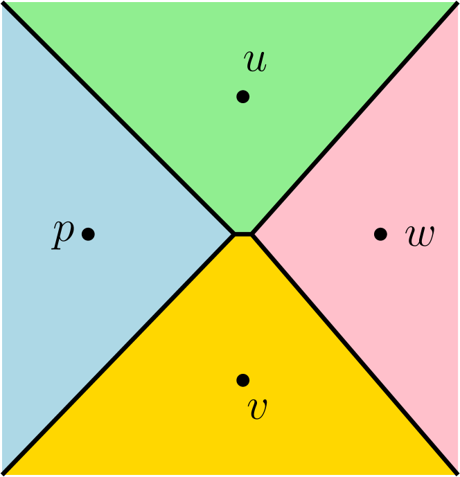
Figure 2: A vertical slice: the $xz$-plane of the initial Voronoi diagram, seen from the negative $y$ axis.

We introduce a number of parameters which we will manipulate to produce the counter-example. We are exploiting the fact that the genericity assumption allows configurations that are arbitrarily close to being degenerate. The assumed $\epsilon_{0}$ has been fixed.

We will work within a coordinate chart on $\mathcal{M}$, where the metric is Euclidean. We will perturb this metric by constructing a metric tensor $\tilde{g}$, and we will denote by $\tilde{\mathcal{M}}$ the manifold with with this new metric.

Consider points $u,v,w,p$ in the $xz$-plane arranged with $u$ and $v$ at $\pm a$ on the $z$ axis, and $w$ and $p$ at $\pm(a+\xi)$ on the $x$ axis, with $a=\frac{3}{4}$, and $0<\xi<r_{0}\gamma$, where $r_{0}$ and $\gamma$ will be specified below. The Voronoi diagram of these points in the $xz$-plane is shown in Figure 2. The main point here is that the Voronoi boundary between $\mathcal{V}_{\mathcal{M}}(u)$ and $\mathcal{V}_{\mathcal{M}}(v)$ may be arbitrarily small with respect to the distance between the sites, i.e., $\xi$ will be very very small.

The three dimensional Voronoi diagram is the extension of this in the horizontal $y$-direction, so that every cross-section looks the same. Note that since the points are not co-circular, they do not represent a degeneracy by Delaunay’s criteria [Del34], but this is irrelevant; we will also argue that the points will not represent a degenerate configuration with respect to the new metric.

We now introduce a small localized metric perturbation so as to change the Voronoi diagram near the origin. For example, we can demand that the matrix of the metric tensor in our coordinate system has the form

$$\tilde{g}(p)=\begin{pmatrix}1-f(\left|p\right|)&0&0\\ 0&1&0\\ 0&0&1\end{pmatrix},$$

where $\left|p\right|$ is the parametric distance from $p$ to the origin. The radial function $f$ is non-negative, and it and its first two derivatives are bounded, e.g.,

$$f(r),\left|f^{\prime}(r)\right|,\left|f^{\prime\prime}(r)\right|\leq\beta.$$ (21)

We also demand that there exists a positive $\gamma\leq\beta$ such that $f(r)\geq\gamma$ when $r\leq r_{0}$, and that $f(r)=0$ if $r\geq 2r_{0}$. The parameter $r_{0}$, defines the radius of the ball bounding the perturbed region. Now we have $d(w,p)<d(u,v)$ when $\xi<r_{0}\gamma$.

Since $\gamma$ may be arbitrarily small compared to $\beta$, standard arguments supply a function $f$ meeting these conditions. For example, the $C^{\infty}$ construction described by Munkres [Mun68, p. 6] may be multiplied by a scalar sufficiently small to meet our needs.

The vertical $y=0$ cross-section of the perturbed Voronoi diagram will look something like Figure 3: $\mathcal{V}_{\tilde{\mathcal{M}}}(p)$ and $\mathcal{V}_{\tilde{\mathcal{M}}}(w)$ now meet in the $xz$-plane, and $\mathcal{V}_{\tilde{\mathcal{M}}}(u)$ and $\mathcal{V}_{\tilde{\mathcal{M}}}(v)$ do not. However, since geodesics which do not intersect the ball $B_{\mathbb{R}^{3}}(0,2r_{0})$ will remain straight lines in the parameter space, the Voronoi diagram is unchanged outside of a neighbourhood of the origin. Thus looking from above at the slice of the Voronoi diagram in the $xy$-plane, we will see something like Figure 4LABEL:sub@sfig:from.above. Figure 4LABEL:sub@sfig:front.view shows the $yz$-plane.

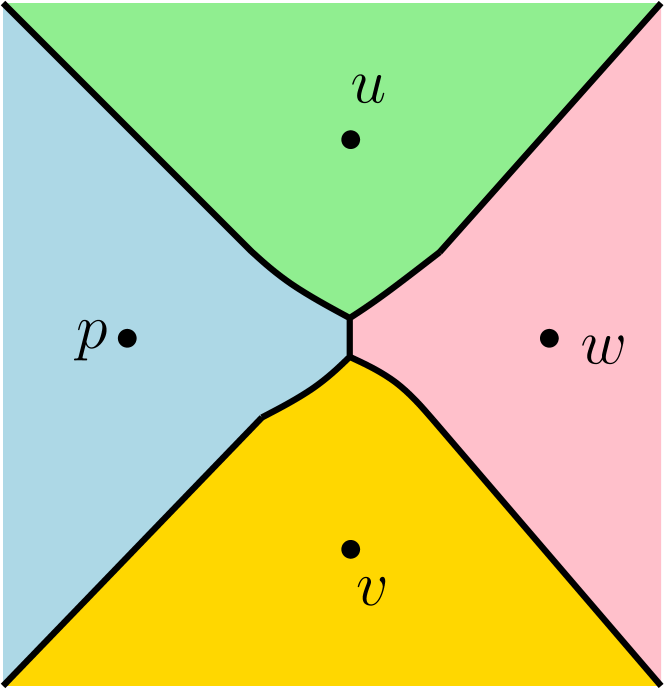
Figure 3: The $y=0$ slice of the perturbed Voronoi diagram.

Two Voronoi vertices have been introduced, the red and blue points in Figure 4. These are the centres of distinct empty geodesic circumballs for $\{p,u,v,w\}$. Since they cannot lie in the region unaffected by the perturbation, a quick calculation shows that the parametric distance of these Voronoi vertices from the origin is bounded by $4r_{0}$, when $r_{0}\leq\frac{1}{4}$, and it follows from another small calculation that the parametric distance from these Voronoi vertices to any of the four sample points is bounded by $a(1+\frac{3\xi+16r_{0}^{2}}{a^{2}})$. The distances between these Voronoi vertices and the sample points in the new metric will also be subjected to the same bound, since no distances increase. Also, The sparsity condition will not be affected by the perturbation. Thus, since we can make $r_{0}$ as small as we please, and $\xi$ is chosen such that $\xi<r_{0}\gamma$, it follows that the radius of these balls may be made arbitrarily close to $a=\frac{3}{4}=\frac{3}{4}\epsilon_{0}\eta(\mathcal{M})$. We will argue next that we can make $\left|\eta(\mathcal{M})-\eta(\tilde{\mathcal{M}})\right|$ as small as desired by reducing the size of $\beta$ in Equation (21). Then other sample points may be placed on the manifold so that the density criteria are met, and no degenerate configuration (violation of Definition A.1) need be introduced.

This means that the Delaunay complex, defined as the nerve of the Voronoi diagram, will not be a triangulation of the manifold $\tilde{\mathcal{M}}$. As observed by Boissonnat et al. [BGO09], the triangle faces $\{p,w,u\}$ and $\{p,w,v\}$ will be adjacent to only a single tetrahedron, namely $\{p,u,v,w\}$. Thus $\operatorname{Del}_{\tilde{\mathcal{M}}}(\mathcal{P})$ is not a manifold complex as defined in Section 2. This is clearly a problem if the original manifold has no boundary.

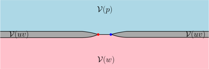
(a) $xy$-plane from above

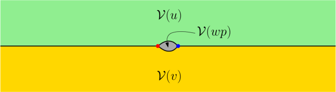
(b) $yz$-plane

Figure 4: Looking at cross-sections; the positive $y$-direction is to the right. The four points, $p,u,v,w$, admit two small circumballs with distinct centres (the red and blue points).

Although it is in some sense close to being degenerate, we emphasise that this configuration represents a problem that cannot be escaped by an arbitrarily small perturbation of the sample points. An argument based on the triangle inequality shows that in order to effect a change in the topology of the Voronoi diagram, a displacement of the points by a distance of $\Omega(r_{0}\gamma-\xi)$ is required.

More specifically, we observe that the configuration $\{p,u,v,w\}$ may be placed in an otherwise well behaved point set $\mathcal{P}$ such that within a small ball centred at the origin in our coordinate chart, all points will have $\{p,u,v,w\}$ as the four closest points in $\mathcal{P}$, and this would remain the case even if the point positions were perturbed a small amount. We may further assume that the other Delaunay simplices are well shaped, so that stability results [BDG12] can be used to argue that they cannot be destroyed with an arbitrarily small perturbation. Then we argue that in order to obtain a triangulation by a perturbation $\mathcal{P}\to\mathcal{P}^{\prime}$, we must ensure that the Voronoi cell $\mathcal{V}_{\tilde{\mathcal{M}}}(\{p^{\prime},w^{\prime}\})$ must vanish: the edge $\{p^{\prime},w^{\prime}\}$ will never be incident to any tetrahedron other than $\{p^{\prime},u^{\prime},v^{\prime},w^{\prime}\}$. Then an argument based on the triangle inequality shows that for a $\rho$-perturbation with $\rho<\frac{r_{0}\gamma-\xi}{6}$, there will be a point in $\mathcal{V}_{\tilde{\mathcal{M}}}(\{p^{\prime},w^{\prime}\})$ within a distance of $2\rho$ of the origin.

A.1.2 The sizing function under perturbation

We need to establish that the metric manipulation that we performed in order to construct the counter-example, does not have a dramatic effect on the sizing function $\eta(\tilde{\mathcal{M}})$. This follows from the fact that we have bounded $g-\tilde{g}$ together with its first and second deriviatives.

Since the sectional curvature may be described as a continuous function of $g$ and it’s first and second derivatives [dC92, pp. 56 & 93], the effect of our perturbation on the sectional curvatures can be made arbitrarily small by reducing $\beta$ in Equation (21).

Since we started with a flat metric anyway, the bound $\mathcal{K}_{0}$ can be made arbitrarily small, and so the second term in Equation (20) will not be the smallest. We need to bound the change in the injectivity radius as well.

This follows from results in the literature [Ehr74, Sak83], which state that for a compact manifold, $\operatorname{inj}(\mathcal{M})$ depends continuously on the metric and its first and second derivatives. Specifically,

Lemma A.4 (Ehrlich).

Let $\mathfrak{M}$ be the space of $C^{3}$ Riemannian metric structures $g$ on a compact manifold $\mathcal{M}$, and endow $\mathfrak{M}$ with the $C^{2}$ topology. The function $g\mapsto\operatorname{inj}_{g}(\mathcal{M})$ is continuous in this topology.

This means that for any desired bound on $\left|\eta(\mathcal{M})-\eta(\tilde{\mathcal{M}})\right|$, there will be a $\beta$ that will satisfy the bound.

The construction of the counter-example is complete.

A.2 Discussion

We have shown that for constructing a Delaunay triangulation for an arbitrary Riemannian manifold, a sampling density requirement is not sufficient in general. The solution we propose in the body of this paper, is to constrain the kind of sample sets that we consider. Another approach would be to constrain the kind of metrics that are assumed. However, even with a purely Euclidean metric, allowing configurations to be arbitrarily close to degeneracy means that arbitrarily poorly shaped simplices are to be expected. When the metric is no longer Euclidean, the “shape” of a simplex no longer has an obvious meaning, but the problems associated with point configurations near degeneracy will certainly be present.

Our analysis relied on the ability to make the support of the perturbation small. This is unlikely to be a necessary feature of the construction, but it facilitates our simplistic analysis.

Clarkson [Cla06] remarked that an implication of Leibon and Letscher’s claim [LL00] is that for four points close enough together, there is a unique circumsphere with small radius. Our counter-example shows that circumcentres need not be unique under these conditions. In fact the existence of unique circumcentres does not follow from the triangulation result: In our work we do not claim that the $m$-simplices have a unique circumcentre in the intrinsic metric. However, the argument sketched out by Leibon and Letscher claimed that the intrinsic Voronoi diagram is a cell complex (i.e., it satisfies the closed ball property [ES97]), and this does imply unique circumcentres for the top dimensional simplices.

It is worth emphasising that the problems discussed here only arise when the dimension is greater than $2$. The same sampling criteria for two dimensional manifolds has been fully validated [Lei99, DZM08], however these works both assume genericity in the sample set, without demonstrating that it is a reasonable assumption.

Appendix B Background results for manifolds

The tangent space at $p\in\mathcal{M}$ is denoted $T_{p}{\mathcal{M}}$, and we identify it with an $m$-flat in the ambient space. The normal space, $N_{p}{\mathcal{M}}$, is the orthogonal complement of $T_{p}{\mathcal{M}}$ in $T_{p}{\mathbb{R}^{N}}$, and we likewise treat it as the affine subspace of dimension $m-k$ orthogonal to $T_{p}{\mathcal{M}}\subset\mathbb{R}^{N}$.

A ball $B=B_{\mathbb{R}^{N}}(c,r)$ is a medial ball at $p$ if $B\cap\mathcal{M}=\emptyset$, it is tangent to $\mathcal{M}$ at $p$, and it is maximal in the sense that any ball which contains $B$ either coincides with $B$ or intersects $\mathcal{M}$. The local reach at $p$ is the infimum of the radii of the medial balls at $p$, and the reach of $\mathcal{M}$, denoted $\text{rch}(\mathcal{M})$, is the infimum of the local reach over all points of $\mathcal{M}$. In order to approximate the geometry and topology with a simplical complex, manifolds with small reach require a higher sampling density than those with a larger reach. As is typical, an upper bound on our sampling radius will be proportional to $\text{rch}(\mathcal{M})$. Since $\mathcal{M}\subset\mathbb{R}^{N}$ is a smooth, compact embedded submanifold, it has positive reach.

An estimate of how the tangent space locally deviates from the manifold is given by an observation of Federer [Fed59, Theorem 4.8(7)] (see also Giesen and Wagner [GW04, Lemma 6]):

Lemma B.1 (Distance to tangent space).

If $x,y\in\mathcal{M}\subset\mathbb{R}^{N}$ and $d_{\mathbb{R}^{N}}(x,y)\leq r<\text{rch}(\mathcal{M})$, then $d_{\mathbb{R}^{N}}(y,T_{x}{\mathcal{M}})\leq\frac{r^{2}}{2\text{rch}(\mathcal{M})}$, and thus $\sin\alpha\leq\frac{r}{2\text{rch}(\mathcal{M})}$, where $\alpha$ is the angle between $[x,y]$ and $T_{x}{\mathcal{M}}$.

A complementary result bounds the distance to the manifold from a point on a tangent space [BG10, Lemma 4.3]:

Lemma B.2 (Distance to manifold).

Suppose $v\in T_{x}{\mathcal{M}}$ with $\left\|v-x\right\|=r\leq\frac{\text{rch}(\mathcal{M})}{4}$. Let $y=\psi_{x}(v)\in\mathcal{M}$, where $\psi_{x}$ is the inverse projection (6). Then, $d_{\mathbb{R}^{N}}(v,y)\leq\frac{2r^{2}}{\text{rch}(\mathcal{M})}$.

The previous two lemmas lead to a convenient bound on the angle between nearby tangent spaces. We prove here a variation on previous results [NSW08, Prop. 6.2] [BG11, Lemma 5.5]:

Lemma B.3 (Tangent space variation).

Let $x,y\in\mathcal{M}$ be such that $d_{\mathbb{R}^{N}}(x,y)=r\leq\frac{\text{rch}(\mathcal{M})}{4}$, and let $\alpha$ be the angle between $T_{x}{\mathcal{M}}$ and $T_{y}{\mathcal{M}}$. Then, $\sin\alpha<\frac{6r}{\text{rch}(\mathcal{M})}.$

Proof.

Let $v\in T_{y}{\mathcal{M}}\subset\mathbb{R}^{N}$ with $\left\|v-y\right\|=r$. We will bound the angle between $v-y$ and $T_{x}{\mathcal{M}}$. We have

$$\begin{split}\sin\alpha&\leq\frac{1}{\left\|v-y\right\|}\left(d_{\mathbb{R}^{N}}(y,T_{x}{\mathcal{M}})+d_{\mathbb{R}^{N}}(v,T_{x}{\mathcal{M}})\right)\\ &\leq\frac{1}{\left\|v-y\right\|}\left(d_{\mathbb{R}^{N}}(y,T_{x}{\mathcal{M}})+d_{\mathbb{R}^{N}}(v,\hat{v})+d_{\mathbb{R}^{N}}(\hat{v},T_{x}{\mathcal{M}})\right),\end{split}$$ (22)

where $\hat{v}\in\mathcal{M}$ is the closest point to $v$ in $\mathcal{M}$.

By Lemma B.1, we have $d_{\mathbb{R}^{N}}(y,T_{x}{\mathcal{M}})\leq\frac{r^{2}}{2\text{rch}(\mathcal{M})}$, and by Lemma B.2 we get $d_{\mathbb{R}^{N}}(v,\hat{v})\leq\frac{2r^{2}}{\text{rch}(\mathcal{M})}$. For the third term in Equation (22), we find

$$\begin{split}d_{\mathbb{R}^{N}}(x,\hat{v})&\leq d_{\mathbb{R}^{N}}(x,y)+\left\|v-y\right\|+d_{\mathbb{R}^{N}}(v,\hat{v})\\ &\leq 2r+\frac{2r^{2}}{\text{rch}(\mathcal{M})}\leq\frac{5r}{2}\\ &<\text{rch}(\mathcal{M}),\end{split}$$

and so we may apply Lemma B.1 to obtain $d_{\mathbb{R}^{N}}(\hat{v},T_{x}{\mathcal{M}})\leq\frac{25r^{2}}{8\text{rch}(\mathcal{M})}$.

Putting these observations back into Equation (22) we find

$$\sin\alpha\leq\frac{1}{\left\|v-y\right\|}\left(\frac{r^{2}}{2\text{rch}(\mathcal{M})}+\frac{2r^{2}}{\text{rch}(\mathcal{M})}+\frac{25r^{2}}{8\text{rch}(\mathcal{M})}\right)=\frac{45r}{8\text{rch}(\mathcal{M})}<\frac{6r}{\text{rch}(\mathcal{M})}.$$

The following observation is a direct consequence of results established by Niyogi et al. [NSW08, Lemma 5.4]:

Lemma B.4.

Let $W=B_{\mathbb{R}^{N}|_{\mathcal{M}}}(p,r)$, for some $p\in\mathcal{M}$ and $r<\text{rch}(\mathcal{M})/2$. When restricted to $W$, the orthogonal projection $\pi_{p}|_{W}:W\to T_{p}{\mathcal{M}}$ is a diffeomorphism onto its image.

Proof.

Let $f=\pi_{p}|_{W}$. Niyogi et al. showed [NSW08, Lemma 5.4] that the Jacobian of $f$ is nonsingular on $W$, so that $W$ is a covering space for $U=f(W)\subset T_{p}{\mathcal{M}}$. The Morse-theory argument of Boissonnat and Chazals [BC01, Proposition 12 ] can be applied to demonstrate that $W$ is a topological ball. It follows that $U$ is connected, since any path in $W$ projects to a path in $U$. Thus $W$ must be a single-sheeted cover of $U$, since $f^{-1}(0)=\{p\}$. Indeed, if $q\in W$ with $q\neq p$ and $f(q)=0$, then $[p,q]$ would be perpendicular to $T_{p}{\mathcal{M}}$, contradicting Lemma B.1. Thus $f:W\to U$ is a diffeomorphism.

Niyogi et al [NSW08, Prop 6.3] demonstrate a bound on the geodesic distance between nearby points, with respect to the ambient distance. We will use a modified statement of this result:

Lemma B.5 (Geodesic distance bound).

Let $x,y\in\mathcal{M}$ be such that $d_{\mathbb{R}^{N}}(x,y)\leq\frac{\text{rch}(\mathcal{M})}{2}$. Then

$$d_{\mathcal{M}}(x,y)\leq d_{\mathbb{R}^{N}}(x,y)\left(1+\frac{2d_{\mathbb{R}^{N}}(x,y)}{\text{rch}(\mathcal{M})}\right).$$

Proof.

The announced result states

$$d_{\mathcal{M}}(x,y)\leq\text{rch}(\mathcal{M})\left(1-\sqrt{1-\frac{2d_{\mathbb{R}^{N}}(x,y)}{\text{rch}(\mathcal{M})}}\right).$$

under the same hypothesis on $x$ and $y$. Rearranging, we have

$$d_{\mathcal{M}}(x,y)\leq\frac{2d_{\mathbb{R}^{N}}(x,y)}{1+\sqrt{1-\frac{2d_{\mathbb{R}^{N}}(x,y)}{\text{rch}(\mathcal{M})}}}\leq\frac{d_{\mathbb{R}^{N}}(x,y)}{1-\frac{d_{\mathbb{R}^{N}}(x,y)}{\text{rch}(\mathcal{M})}}\leq d_{\mathbb{R}^{N}}(x,y)\left(1+\frac{2d_{\mathbb{R}^{N}}(x,y)}{\text{rch}(\mathcal{M})}\right),$$

where the second inequality is obtained by squaring away the radical.

Appendix C Forbidden volume calculation

In this appendix we demonstrate:

Lemma 5.8(Volume of forbidden region) Let $\sigma$ be a $k$-simplex with vertices on $\mathcal{M}$ and $k\leq m$. If

1. $\Gamma_{0}\leq\frac{1}{B+1}$,

2. $\tilde{\epsilon}\leq\min\{\frac{\xi}{4\beta\,\text{rch}(\mathcal{M})},\,\frac{\Gamma^{m+1}_{0}}{8\beta}\}$ and

3. $\delta_{0}^{2}\leq\min\{\Gamma_{0}^{m+1},\frac{1}{4}\}$,

then

$$\operatorname{vol}(F(\sigma,t))\leq D\,\Gamma_{0}\,R(\sigma)^{m},$$

where $D$ depends on $m$ and $\beta$.

We will use the following lemmas in the proof of Lemma 5.8:

Lemma C.1 (Triangle altitude bound).

For any non-degenerate triangle $\sigma=[p,q,r]$, we have

$$D(p,\sigma)=\frac{\|p-q\|\|p-r\|}{2R(\sigma)}.$$

Proof.

Let $\alpha=\angle prq$ and observe that

$$\sin\alpha=\frac{\|p-q\|}{2R(\sigma)}.$$

Since $D(p,\sigma)=\|p-r\|\sin\alpha$, the result follows.

Lemma C.2.

Let $\sigma=[p_{0}\,\dots\,p_{k}]\subset\mathbb{R}^{N}$ be a $k$-simplex with $1\leq k\leq m<N$. Suppose $p_{k+1}\in\mathbb{R}^{N}$ is such that $\sigma_{1}=p_{k+1}*\sigma$ admits an elementary weight function $\omega_{\sigma_{1}}:\mathring{\sigma_{1}}\rightarrow[0,\infty)$, and the following conditions are satisfied:

1. $L(\sigma_{1})>\frac{t}{9}$,

2. $R(\sigma_{1},\omega_{\sigma_{1}})<\beta t$,

3. $\sigma_{1}$ is a $\Gamma_{0}$-flake, and

4. $\delta^{2}_{0}\leq\min\{\Gamma^{m+1}_{0},\,\frac{1}{4}\}$.

Then

$$d_{\mathbb{R}^{N}}(p_{k+1};\partial S^{\prime})\leq B\,\Gamma_{0}R(\sigma)$$

where $S^{\prime}=B_{\mathbb{R}^{N}}(C(\sigma),R(\sigma))\cap\operatorname{aff}(\sigma)$ and

$$B\;\stackrel{{\scriptstyle{\rm def}}}{{=}}4+96\beta(1+2^{7}3^{2}\beta^{2}).$$

Proof.

Let $\omega_{\sigma}=\omega_{\sigma_{1}}\mid_{\mathring{\sigma}}$. Note that $\omega_{\sigma}:\mathring{\sigma}\rightarrow[0,\infty)$ is an elementary weight function, and $C(\sigma,\omega_{\sigma})$ is the orthogonal projection of $C(\sigma_{1},\omega_{\sigma_{1}})$ onto $\operatorname{aff}(\sigma)$.

From Lemma 4.1 (2) and the fact that $\delta^{2}_{0}\leq\frac{1}{4}$, we have

$$\Delta(\sigma_{1})\leq\frac{2}{1-\delta^{2}_{0}}R(\sigma_{1},\omega_{\sigma_{1}})<\frac{8}{3}R(\sigma_{1},\omega_{\sigma_{1}}).$$ (23)

and

$$\frac{R(\sigma,\omega_{\sigma})}{R(\sigma_{1},\omega_{\sigma_{1}})} \geq\frac{(1-\delta^{2}_{0})\Delta(\sigma)}{2R(\sigma_{1},\omega_{\sigma_{1}})}$$ from Lemma 4.1 (2)

$$\geq\frac{3L(\sigma)}{8R(\sigma_{1},\omega_{\sigma_{1}})} \delta_{0}^{2}\leq\frac{1}{4} L(\sigma)\leq\Delta(\sigma)$$ as and

$$\geq\frac{1}{24\beta}$$ (24)

Therefore, from Lemma 2.7, we have

$$\frac{D(p_{k+1},\sigma_{1})}{\Delta(\sigma)} <\left(1+\frac{1}{k}\right)\Gamma_{0}\times\frac{\Delta(\sigma_{1})^{2}}{L(\sigma_{1})\Delta(\sigma)}$$

$$\leq 2\Gamma_{0}\times\frac{\Delta(\sigma_{1})^{2}}{L(\sigma_{1})^{2}} k\geq 1 L(\sigma_{1})\leq\Delta(\sigma)$$ from and

$$<\frac{128\Gamma_{0}}{9}\times\frac{R(\sigma_{1},\omega_{\sigma_{1}})^{2}}{L(\sigma_{1})^{2}}$$ from Eq. (23)

$$<2^{7}3^{2}\beta^{2}\times\Gamma_{0}$$ from hyp. (1) & (2) (25)

Let $p$ be the point closest to $p_{k+1}$ in $\partial B_{\mathbb{R}^{N}}(C;R)$ where $C=C(\sigma_{1},\omega_{\sigma_{1}})$ and $R=R(\sigma_{1},\omega_{\sigma_{1}})$. We have

$$\|p-p_{k+1}\|=\sqrt{R^{2}+\omega_{\sigma_{1}}(p_{k+1})^{2}}-R\leq\omega_{\sigma_{1}}(p_{k+1})\leq\delta_{0}L(\sigma_{1})$$ (26)

Let $q$ be the point closest to $p$ on $\partial B_{\mathbb{R}^{N}}(C;R)\cap\operatorname{aff}(\sigma)$, $p^{\prime}$ be the projection of $p$ onto $\operatorname{aff}(\sigma)$, and and let $r$ denotes the intersection of the line $\operatorname{aff}([q\,C(\sigma,\omega_{\sigma})])$ with $\partial B_{\mathbb{R}^{N}}(C;R)$. Note that $C(\sigma_{1},\omega_{\sigma_{1}})$, $C(\sigma,\omega_{\sigma})$, $p_{k+1}$, $p$, $p^{\prime}$, $q$ and $r$ lie on the same $2$-dimensional affine space.

Using the fact that $\|p-p_{k+1}\|\leq\delta_{0}L(\sigma_{1})$, we get

$$\|p-p^{\prime}\|\leq D(p_{k+1},\sigma_{1})+\delta_{0}L(\sigma_{1})$$ (27)

We will now consider the triangle $\sigma_{2}=[p\,q\,r]$. Note that $C(\sigma_{1},\omega_{\sigma_{1}})$, $R(\sigma_{1},\omega_{\sigma_{1}})$ are the circumcenter and radius of $\sigma_{2}$ respectively. Also, $C(\sigma,\omega_{\sigma})$ is the midpoint of the line segment $[q\,r]$ with $2R(\sigma,\omega_{\sigma})=\|q-r\|$ and $D(p,\sigma_{2})=\|p-p^{\prime}\|$. From the definition of $q$, we have $\|p-r\|\geq\|p-q\|$. Using the fact $\|q-r\|=2R(\sigma,\omega_{\sigma})$, we have

$$\|p-r\|\geq\frac{\|q-r\|}{2}=R(\sigma,\omega_{\sigma}).$$

This implies from Lemma C.1

$$\|p-q\| =\frac{2R(\sigma_{2})D(p,\sigma_{2})}{\|p-r\|}$$

$$\leq\frac{2R(\sigma_{1},\omega_{\sigma_{1}})D(p,\sigma_{2})}{R(\sigma,\omega_{\sigma})} R(\sigma_{2})\leq R(\sigma_{1},\omega_{1}) \|p-r\|\geq R(\sigma,\omega_{\sigma})$$ as and

$$\leq 48\beta D(p,\sigma_{2})=48\beta\|p-p^{\prime}\|$$ as Eq. (C) (28)

From Eq. (26), (27) and (C)

$$\|p_{k+1}-q\| \leq\|p_{k+1}-p\|+\|p-q\|$$

$$\leq\delta_{0}L(\sigma_{1})+48\beta(D(p_{k+1},\sigma_{1})+\delta_{0}L(\sigma_{1}))$$

$$\stackrel{{\scriptstyle{\rm def}}}{{=}}\eta_{1}$$ (29)

Using the fact that $\sigma$ is $\Gamma^{k}_{0}$-thick (since $\sigma_{1}$ is a $\Gamma_{0}$-flake), and the bound $\delta_{0}^{2}L(\sigma_{1})^{2}$ on the differences of the squared distances between $C(\sigma,\omega_{\sigma})$ and the vertices of $\sigma$, we obtain a bound [BDG12, Lemma 4.1] on the distance from $C(\sigma,\omega_{\sigma})$ to $C(\sigma)$:

$$\|C(\sigma)-C(\sigma,\omega_{\sigma})\| \leq\frac{\delta_{0}^{2}L(\sigma_{1})^{2}}{2\Upsilon(\sigma)\Delta(\sigma)}$$

$$\leq\frac{\delta^{2}_{0}R(\sigma)}{\Upsilon(\sigma)} L(\sigma_{1})\leq\Delta(\sigma)\leq 2R(\sigma)$$ as

$$\leq\frac{\delta^{2}_{0}R(\sigma)}{\Gamma_{0}^{k}} \sigma \Gamma^{k}_{0} \Upsilon(\sigma)\geq\Gamma^{k}_{0}$$ since is -thick,

$$\leq\frac{\delta^{2}_{0}R(\sigma)}{\Gamma_{0}^{m}} \Gamma_{0}\leq 1$$ as

$$\stackrel{{\scriptstyle{\rm def}}}{{=}}\eta_{2}$$ (30)

Since $k\geq 1$, there exists $p_{i}\in\mathring{\sigma}$ such that

$$p_{i}\in B_{\mathbb{R}^{N}}(C(\sigma),R(\sigma))\cap B_{\mathbb{R}^{N}}(C(\sigma,\omega_{\sigma}),R(\sigma,\omega_{\sigma}))\cap\operatorname{aff}(\sigma).$$

Also, $\|C(\sigma)-p_{i}\|=R(\sigma)$ and $\|C(\sigma,\omega_{\sigma})-p_{i}\|=R(\sigma,\omega_{\sigma})$.

Using the facts that $R(\sigma)=\|C(\sigma)-p_{i}\|$ and $R(\sigma,\omega_{\sigma})=\|C(\sigma,\omega_{\sigma})-p_{i}\|$, and the Triangle inequality, we get

$$R(\sigma)-\|C(\sigma)-C(\sigma,\omega_{\sigma})\|\;\;\leq \|C(\sigma,\omega_{\sigma})-p_{i}\| \leq\;\;R(\sigma)+\|C(\sigma)-C(\sigma,\omega_{\sigma})\|$$

$$R(\sigma)-\eta_{2}\;\;\leq R(\sigma,\omega_{\sigma}) \leq\;\;R(\sigma)+\eta_{2}$$ (31)

The last equation follows from Eq. (C).

Let $S^{\prime}$ and $S$ denote $B_{\mathbb{R}^{N}}(C(\sigma),R(\sigma))\cap\operatorname{aff}(\sigma)$ and $B_{\mathbb{R}^{N}}(C(\sigma,\omega_{\sigma}),R(\sigma,\omega_{\sigma}))$ respectively. From Eq. (C) and (C), we have $d_{\mathbb{R}^{N}}(\partial S^{\prime},\partial S)\leq\eta_{1}+2\eta_{2}$. This implies that there exists $q^{\prime}\in\partial S^{\prime}$ such that

$$\|q^{\prime}-q\|\leq 2\eta_{2}.$$ (32)

Therefore from Eq. (C) and (32), we get

$$\|p_{k+1}-q^{\prime}\|\leq\|p_{k+1}-q\|+\|q^{\prime}-q\|\leq\eta_{1}+2\eta_{2}$$

Using the facts that $\delta^{2}_{0}\leq\Gamma_{0}^{m+1}\leq\Gamma^{2}_{0}$ (from hyp. (4) of the lemma and $\Gamma_{0}\leq 1$), $L(\sigma_{1})\leq L(\sigma)\leq\Delta(\sigma)\leq 2R(\sigma)$ and $\frac{D(p_{k+1},\sigma_{1})}{\Delta(\sigma)}\leq 2^{7}3^{2}\beta^{2}\,\Gamma_{0}$ (from Eq. (C)), and Eq. (C) and (C), we get

$$d_{\mathbb{R}^{N}}(p_{k+1};\partial S^{\prime}) \leq \|p_{k+1}-q^{\prime}\|$$

$$\leq \eta_{1}+2\eta_{2}$$

$$\leq \delta_{0}L(\sigma_{1})+48\beta\left(D(p_{k+1},\sigma_{1})+\delta_{0}L(\sigma_{1})\right)+\frac{2\delta^{2}_{0}R(\sigma)}{\Gamma^{m}_{0}}$$

$$\leq B\Gamma_{0}R(\sigma)$$

where

$$B=4+96\beta(1+2^{7}3^{2}\beta^{2}).$$

We will use the following lemma from [BG10] to bound the volume of $F(\sigma)$.

Lemma C.3.

Let $p$ be a point on $\mathcal{M}$. There exists $\xi$ that depends on $\text{rch}(\mathcal{M})$ and $m$, and $A$ that depends only on $m$ such that, for all $r=t\leq\xi$, we have

$$0<1-A\,\tilde{t}\leq\frac{\operatorname{vol}(B_{\mathbb{R}^{N}}(p,r)\cap\mathcal{M})}{V_{m}r^{k}}\leq 1+A\,\tilde{t}$$

where $V_{m}$ is the volume of the $m$-dimensional unit Euclidean ball.

of Lemma 5.8.

For the rest of the proof we define

$$\tilde{t}=\frac{t}{\text{rch}(\mathcal{M})}$$

Consider the following elementary weight function: $\omega_{\sigma}=\omega_{\sigma_{1}}\mid_{\mathring{\sigma}}$. Using the facts that $R(\sigma,\omega_{\sigma})\leq R(\sigma_{1},\omega_{\sigma_{1}})$, $R(\sigma,\omega_{\sigma})<\beta t\,\text{rch}(\mathcal{M})$, and Lemma 4.1 (3)

$$R(\sigma) \leq R(\sigma,\omega_{\sigma})\left(1-\frac{\delta^{2}_{0}}{\Upsilon(\sigma)}\right)^{-1}$$

$$\leq R(\sigma,\omega_{\sigma})\left(1-\frac{\delta^{2}_{0}}{\Gamma_{0}^{m}}\right)^{-1} \Upsilon(\sigma)\geq\Gamma^{k}_{0}\geq\Gamma^{m}_{0}$$ since

$$\leq 2\beta\tilde{t}\,\text{rch}(\mathcal{M})$$ (33)

Let $p$ be a vertex of $\sigma$. Let $c$ be the point closest to $C(\sigma)$ on $T_{p}\mathcal{M}$ and $c^{*}$ be the point closest to $c$ on $\mathcal{M}$ (see Fig. 5).

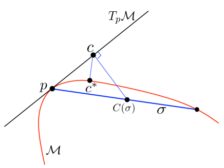
Figure 5: Proof of Lemma 5.8.

From Lemma B.1, we have for all $q\in\mathring{\sigma}$

$$d_{\mathbb{R}^{m}}(q,T_{p}\mathcal{M})\leq\frac{\|p-q\|^{2}}{2\text{rch}(\mathcal{M})}\leq\frac{\Delta(\sigma)^{2}}{2\,\text{rch}(\mathcal{M})}\stackrel{{\scriptstyle{\rm def}}}{{=}}\eta$$

From Lemma 2.1, and the facts that $\Upsilon(\sigma)\geq\Gamma^{m}_{0}$ and $\Delta(\sigma)\leq 2R(\sigma)\leq 4\beta t$, we have

$$\sin\angle(T_{p}\mathcal{M},\operatorname{aff}(\sigma))\leq\frac{2\eta}{\Upsilon(\sigma)\Delta(\sigma)}\leq\frac{\Delta(\sigma)}{\Upsilon(\sigma)\text{rch}(\mathcal{M})}\leq\frac{4\beta\,\tilde{t}}{\Gamma_{0}^{m}}$$

Therefore

$$\|c-C(\sigma)\|\leq\sin\angle(T_{p}\mathcal{M},\operatorname{aff}(\sigma))\times R(\sigma)\leq\left(\frac{4\beta\,\tilde{t}}{\Gamma^{m}_{0}}\right)R(\sigma),$$ (34)

and from Lemma 4.2

$$\|c-c^{*}\|\leq\frac{2\|c-p\|^{2}}{\text{rch}(\mathcal{M})}\leq 4\beta\tilde{t}\,R(\sigma).$$ (35)

Let $x\in F(\sigma,t)$ and $x^{*}$ be the point closest to $x$ on $\partial\,B_{\mathbb{R}^{N}}(C(\sigma),R(\sigma))\cap\operatorname{aff}(\sigma)$. Then from Lemma C.2, we have

$$\|x-x^{*}\|<B\Gamma_{0}R(\sigma)$$ (36)

Using the fact that $\|C(\sigma)-x^{*}\|=R(\sigma)$, we get

$$\|c^{*}-x\| \leq\|c^{*}-c\|+\|c-C(\sigma)\|+\|C(\sigma)-x^{*}\|+\|x^{*}-x\|$$

$$<R(\sigma)\left(1+B\Gamma_{0}+4\beta t\,\left(\frac{1}{\Gamma^{m}_{0}}+1\right)\right)$$ from Eq. (34), (35), (36)

$$\leq R(\sigma)\left(1+B\Gamma_{0}+\frac{8\beta\,\tilde{t}}{\Gamma^{m}_{0}}\,\right) \Gamma_{0}\leq 1$$ since

$$\leq R(\sigma)(1+(B+1)\Gamma_{0})$$ from hyp. 2 of the lemma.

Similarly we can show that

$$\|c^{*}-x\|<R(\sigma)(1-(B+1)\Gamma_{0})$$

Therefore

$$F(\sigma,t)\subseteq\left(B_{\mathbb{R}^{N}}(c^{*},(1+\zeta)R(\sigma))\setminus B_{\mathbb{R}^{N}}(c^{*},(1-\zeta)R(\sigma))\right)\cap\mathcal{M}$$

where $\zeta=(B+1)\Gamma_{0}$.

Observe that Lemma C.3 can be applied since

$$R(\sigma)(1+\zeta) \leq 2R(\sigma) \zeta\leq 1$$ since from hyp. 1

$$\leq 4\beta t$$ from Eq. (C)

$$\leq\xi t<\epsilon$$ because .

Therefore

$$\frac{\operatorname{vol}(F(\sigma,t))}{V_{m}} \leq \frac{\operatorname{vol}(B_{\mathbb{R}^{N}}(c^{*},R(\sigma)(1+\zeta))\cap\mathcal{M}\setminus B_{\mathbb{R}^{N}}(c^{*},R(\sigma)(1-\zeta))\cap\mathcal{M})}{V_{m}}$$ (37)

$$\leq (1+A(1+\zeta)\tilde{t}\,)R(\sigma)^{m}(1+\zeta)^{m}-(1-A(1-\zeta)\tilde{t}\,)R(\sigma)^{m}(1+\zeta)^{m}$$

$$\leq R(\sigma)^{m}((1+\zeta)^{m}-(1-\zeta)^{m})+A\tilde{t}R(\sigma)^{m}((1+\zeta)^{m}+(1-\zeta)^{m})$$

$$\leq 2^{m}\zeta\,R(\sigma)^{m}+A(2^{m+1}+1)\tilde{t}\,R(\sigma)^{m}$$

The last inequality follows from the fact that $(1+x)^{m}-(1-x)^{m}\leq 2^{m}x$ for all $x\in[0,1]$.

From hyp. 2 and the fact that $\Gamma_{0}<1$, we have

$$\tilde{t}\leq\tilde{\epsilon}\leq\frac{\Gamma_{0}^{m+1}}{8\beta}<\Gamma_{0}.$$ (38)

The lemma now follows from Eq. (37) and (38).

References

• [BC01] J.-D. Boissonnat and F. Cazals. Natural neighbour coordinates of points on a surface. Computational Geometry Theory and Applications, 19(2):155–173, 2001.
• [BDG12] J.-D. Boissonnat, R. Dyer, and A. Ghosh. The stability of Delaunay triangulations, 2012. submitted to Int. J. Comp. Geom. & Appl. (special issue for SoCG).
• [BG10] J.-D. Boissonnat and A. Ghosh. Triangulating smooth submanifolds with light scaffolding. Mathematics in Computer Science, 4(4):431–461, 2010.
• [BG11] J.-D. Boissonnat and A. Ghosh. Manifold reconstruction using tangential Delaunay complexes. Technical Report $N^{\circ}$ 7142 v.3, INRIA, 2011.
• [BGO09] J.-D. Boissonnat, L. J. Guibas, and S. Y. Oudot. Manifold reconstruction in arbitrary dimensions using witness complexes. Discrete & Comp. Geom., 42:37–70, 2009.
• [BWY11] J.-D. Boissonnat, C. Wormser, and M. Yvinec. Anisotropic Delaunay mesh generation. Research Report RR-7712, INRIA, 2011.
• [CDE+00] S.-W. Cheng, T. K. Dey, H. Edelsbrunner, M. A. Facello, and S. H Teng. Sliver exudation. Journal of the ACM, 47(5):883–904, 2000.
• [CDR05] S.-W. Cheng, T. K. Dey, and E. A. Ramos. Manifold reconstruction from point samples. In SODA, pages 1018–1027, 2005.
• [Cha06] I. Chavel. Riemannian Geometry, A modern introduction. Cambridge, 2nd edition, 2006.
• [Cla06] K. L. Clarkson. Building triangulations using epsilon-nets. In STOC. ACM Press, 2006.
• [dC92] M. P. do Carmo. Riemannian Geometry. Birkhäuser, 1992.
• [Del34] B. Delaunay. Sur la sphère vide. Izv. Akad. Nauk SSSR, Otdelenie Matematicheskii i Estestvennyka Nauk, 7:793–800, 1934.
• [DZM08] R. Dyer, H. Zhang, and T. Möller. Surface sampling and the intrinsic Voronoi diagram. Computer Graphics Forum (Special Issue of Symp. Geometry Processing), 27(5):1393–1402, 2008.
• [Ehr74] P. Ehrlich. Continuity properties of the injectivity radius function. Composito Mathematica, 29:151–178, 1974.
• [ES97] H. Edelsbrunner and N. R. Shah. Triangulating topological spaces. Int. J. Comput. Geometry Appl., 7(4):365–378, 1997.
• [Fed59] H. Federer. Curvature measures. Trans. Amer. Math. Soc., 93(3):418–491, 1959.
• [GW04] J. Giesen and U. Wagner. Shape dimension and intrinsic metric from samples of manifolds. Discrete & Comp. Geom., 32:245–267, 2004.
• [Lei99] G. Leibon. Random Delaunay triangulations, the Thurston-Andreev theorem, and metric uniformization. PhD thesis, UCSD, 1999. arXiv:math/0011016v1.
• [Li03] X-Y. Li. Generating well-shaped $d$-dimensional Delaunay meshes. Theoretical Computer Science, 296(1):145–165, 2003.
• [LL00] G. Leibon and D. Letscher. Delaunay triangulations and Voronoi diagrams for Riemannian manifolds. In SoCG, pages 341–349, 2000.
• [LS03] F. Labelle and J. R. Shewchuk. Anisotropic Voronoi diagrams and guaranteed-quality anisotropic mesh generation. In SoCG, pages 191–200, 2003.
• [Mun68] J. R. Munkres. Elementary differential topology. Princton University press, second edition, 1968.
• [Mun84] J. R. Munkres. Elements of Algebraic Topology. Addison-Wesley, 1984.
• [NSW08] P. Niyogi, S. Smale, and S. Weinberger. Finding the homology of submanifolds with high confidence from random samples. Discrete & Comp. Geom., 39(1-3):419–441, 2008.
• [Sak83] T. Sakai. On continuity of injectivity radius function. Mathematical Journal of Okayama University, 25(1):91–97, 1983.
• [Whi57] H. Whitney. Geometric Integration Theory. Princeton University Press, 1957.