The electrostatic interaction of an external charged system with a metal surface: a simplified density functional theory approach

Abstract

As a first step to meet the challenge to calculate the electronic structure and total energy of charged states of atoms and molecules adsorbed on ultrathin-insulating films supported by a metallic substrate using density functional theory (DFT), we have developed a simplified new DFT scheme that only describes the electrostatic interaction of an external charged system with a metal surface. This purely electrostatic interaction is obtained from the assumption that the electron densities of the two fragments (charged system and metal surface) are non-overlapping and neglecting non-local exchange correlation effects such as the van der Waals interactions between the two fragments. In addition, the response of the metal surface to the electrostatic potential from the charged system is treated to linear order, whereas the charged system is treated fully within DFT. In particular, we consider the classical perfect conductor (PC) model for the metal response, although our formalism is not limited to this approximation. The successful computational implementation of this new methodology and the PC model is exemplified by the case of a Na⁺ cation outside a metal surface.

Keywords Electronic structure calculations and methods, Density functional theory, Charged systems, Metal surfaces

1 Introduction

Recent progress in the studies of single atoms and molecules on ultrathin-insulating films supported by a metal substrate have opened up a new frontier in atomic scale science. Not only are these films able to decouple the electronic states of the adsorbates from the metal substrate states, but they also provide sufficient tunnelling current to be able to characterise, manipulate and image the adsorbed species by a scanning tunnelling microscope. Some important examples include charge state control of adsorbed species [1, 2], imaging of frontier orbitals [3, 4], coherent electron-nuclear coupling in molecular wires [5] and tunnelling-induced switching of adsorbed molecules [6, 7]. In particular, polar films such as NaCl bilayers are able to support multiple charge states of adsorbed species, which can be switched in a controlled manner by attachment and detachment of tunnelling electrons. Furthermore, these processes have been suggested to be responsible for the observed reversible bond formation in molecular switches [7]. To fully exploit the new potential opportunities provided by these systems, there is a need of theory to unravel the electronic and geometric structure and the excited state potentials of anionic and cationic states of the adsorbed species.

Some important advances in this respect have been made by using Density Functional Theory (DFT) [8, 9] calculations [1, 14, 4, 2, 7]. However, the delocalisation error in the current exchange-correlation functionals and the system size make the calculations very challenging. In fact, this error in current density functionals can result in fractional occupation of the adsorbed species and makes it difficult to identify various multiply charged states [10]. Even with these limitations, important progress has been made by using DFT+U [11, 12] to correct for the self-interaction behind the delocalisation error for a Ag atom [2], despite it is generally a bit dubious for delocalised states such as for $s$ states of atoms [13]. There has also been some developments in constraining the occupancy of adsorbate orbitals, but this requires that one has to identify the appropriate Kohn-Sham orbital, which can still be challenging due to the mixing of adsorbate and substrate states albeit being very small [14]. However, when considering, for example, organic molecules adsorbed on an ultrathin-insulating film supported by a metal surface, the number of metal atoms and the associated number of metal electrons makes the calculations to become prohibitively large.

As a first step to try to overcome these limitations, we present a new simplified DFT method for the calculation of the total energy, ionic (Hellman-Feynman) forces and electronic structure of a charged system placed in front of a metal surface. In this method, the charged system is fully treated using DFT, the interaction between the two systems is assumed to be electrostatic and the density response of the metal surface to the electrostatic interaction is treated to linear order. The proposed method has two main advantages. Firstly, the computational effort is significantly decreased, since the metal electron states are not treated explicitly but only implicitly through their density response to an external electrostatic field, which can be captured using a simple model. Here, we have explicitly considered the classical perfect conductor (PC) model for the metal response in which the screening length by the conduction electrons is assumed to be zero and the screening charge only resides on the perfect conductor plane. Secondly, different charge states of the charged system can be handled directly using this method.

We have implemented this new methodology in the VASP code [23] using the simple PC model for the metal response. A critical test of this implementation is provided by the example of the Na⁺ ion outside a perfect conductor. Here, the six electrons in the $p$ semi-core of the Na⁺ ion were included in the calculations. The results show an excellent agreement between the calculated Hellman-Feynman force on the ion and the negative gradient of the interaction energy even in the region close to the perfect conductor plane, where the electron density of the ion overlaps with the induced charge density at perfect conductor plane. Furthermore, the small polarisability of the ion makes the calculated interaction energy to be in close agreement with the analytical result for a point charge model outside the perfect conductor.

In applying this method to study charged adsorbates deposited over ultrathin-insulating films supported by a metal substrate, we need to extend the PC model by including the interactions between the film and the metal substrate arising from overlapping electron densities and van der Waals interactions. We plan to capture these interactions through a simple parametrised force field between the metal substrate and the ions in the film, where parameters will be obtained by fitting the force field to DFT calculations of the forces between the film (without adsorbates) and the metal substrate. A successful implementation of this force field should enable us to describe, for example, the observed reversible bond formation of a molecular switch induced by a tunnelling electron and hole attachment to form ionic adsorbate states [7]. The presentation of this scheme and associated results are deferred to a future publication.

This paper is organised as follows. In the next Section 2, we present the theoretical background of the proposed method. First, the effective energy density functional and the associated Hellman-Feynman forces for the charged system are derived in Subsection 2.1 under the assumption that the electrons of the charged system and the metal surface are distinguishable. The total energy of the metal surface is expanded up to second order in the resulting electrostatic interaction between the two systems. In the next Subsection 2.2, the non-trivial effects on the electrostatics when imposing periodic boundary conditions are analysed and appropriate dipole corrections for the total energy and the Hellman-Feynman forces are derived. The classical perfect conductor model for the metal surface response is then introduced in the next Subsection 2.3. Here, we also present analytical expressions for the interaction energy and force in the case of a point charge (Subsection 2.3.1) in the presence of periodic boundary conditions, and discuss possible refinements of the perfect conductor model (Subsection 2.3.2). In Section 3, the keys steps in implementing the PC model in the plane wave code VASP are presented. As a first test of this methodology, we show the results of the computational implementation of the PC model for the case of Na⁺ ion outside a PC (Section 4) and finally give some concluding remarks in Section 5.

2 Theoretical framework

In this Section we develop a density functional theoretical description of a charged system placed in front of a metal surface based on the assumption that the electrons of both fragments are distinguishable, so that the interaction between the two systems is only electrostatic. The corresponding approximation becomes valid when the electron densities of the two systems are well separated. We analyse how the system can be treated in a supercell geometry and derive expressions for the dipole correction of the Kohn-Sham potential and the Hellmann-Feynman forces. As an explicit model for the metal surface, we focus on the classical perfect conductor (PC) model of the metal surface response, but also discuss possible extensions of this approximation. For the particular case of a point charge, we present explicit expressions for the interaction energy with a perfect conductor. Throughout the paper, we will make use of electrostatic units.

2.1 Approximate energy density functional

We consider a closed, charged system $S$ of electrons and ions outside a metal surface $M$. In contrast to the system $S$, the metal surface will be treated as an open system, kept at a constant chemical potential $\mu$. The electron densities of $S$ and $M$ are assumed to be non-overlapping and are given by $n_{s}({\bf r})$ and $n_{m}({\bf r})$, respectively. In this case the kinetic energy functional of the non-interacting electrons is additive in the electron densities of $S$ and $M$. Furthermore, we will neglect any non-local contributions between $S$ and $M$ such as the van der Waals interaction so that the exchange-correlation energy functional is also additive in these electron densities. The total energy density functional for the combined system is then given by the following expression:

$$E[n_{m},n_{s}]=E_{s}[n_{s}]+E_{m}[n_{m}]-\mu N_{m}+\int\rho_{m}({\bf r})\phi_{s}({\bf r})d{\bf r}\ .$$ (1)

Here $E_{s}[n_{s}]$ and $E_{m}[n_{m}]$ are the energy density functionals for the isolated $S$ and $M$, respectively, whereas $\rho_{m}({\bf r})$ is the charge density of $M$ and $N_{m}$ the total number of electrons of $M$. The potential $\phi_{s}({\bf r})$ is defined as the electrostatic potential generated from the total charge density $\rho_{s}({\bf r})=-en_{s}({\bf r})+\rho_{i}({\bf r})$ of electrons and ions in $S$ and is given by,

$$\phi_{s}({\bf r})=\int\frac{\rho_{s}({\bf r^{\prime}})d{\bf r^{\prime}}}{|{\bf r}-{\bf r^{\prime}}|}\ .$$ (2)

Note that the approximation in Eqn.(1) is still meaningful for overlapping electron densities. Furthermore, any neglected non-additive contributions to the kinetic energy and the exchange-correlation potential including any non-local contribution between $M$ and $S$, such as the van der Waals interaction, will be accounted by introducing a force field between $M$ and $S$.

An effective total energy density functional for $S$ outside $M$ in term of the electron density $n_{s}({\bf r})$ is obtained by minimising the energy density functional in Eqn.(1) with respect to $n_{m}$ for fixed $n_{s}$ and $\mu$,

$$\frac{\delta E_{m}}{\delta n_{m}({\bf r})}=\mu+e\phi_{s}({\bf r})$$ (3)

and, since $\mu$ is constant, we conclude that the ground state electron density of $M$ in the presence of $S$ is a functional of $n_{s}$, i. e. $n_{m}=n_{m}[n_{s}]$. The change in energy of $M$ induced by the presence of $S$ is defined as,

$$\Delta E_{m}[n_{s}] = (E_{m}[n_{m}]-E_{m}[n_{m0}])-\mu(N_{m}-N_{m0})+\int\rho_{m}({\bf r})\phi_{s}({\bf r})d{\bf r}$$ (4)

where $n_{m0}$ and $N_{m0}$ are the unperturbed ground state electronic density and total number of electrons of $M$, respectively. Expanding $\Delta E_{m}[n_{s}]$ up to second order in $\phi_{s}({\bf r})$, one obtains

$$\Delta E_{m}[n_{s}] = \int\frac{\delta\Delta E_{m}}{\delta\phi_{s}({\bf r})}\phi_{s}({\bf r})d{\bf r}+\frac{1}{2}\int\int\frac{\delta^{2}\Delta E_{m}}{\delta\phi_{s}({\bf r})\delta\phi_{s}({\bf r}^{\prime})}\phi_{s}({\bf r})\phi_{s}({\bf r}^{\prime})d{\bf r}d{\bf r}^{\prime}.$$ (5)

The two terms in Eqn.(5) can now be cast in a more familiar form using the result

$$\rho_{m}({\bf r})=\frac{\delta\Delta E_{m}}{\delta\phi_{s}({\bf r})}\ ,$$ (6)

which follows from the fact that $\Delta E_{m}[n_{s}]$, defined in Eqn.(4), is stationary with respect to variations in $n_{m}({\bf r})$ for fixed $\phi_{s}$ . Thus, the first term of the r.h.s in Eqn.(5) is determined by the unperturbed charge density $\rho_{m0}$ of the metal $M$, whereas the second term is given by the induced charge density $\rho_{ind}({\bf r})$ in $M$, which, to linear order in $\phi_{s}$, is given by

$$\rho_{ind}({\bf r})=\int\frac{\delta\rho_{m}({\bf r})}{\delta\phi_{s}({\bf r^{\prime}})}\phi_{s}({\bf r^{\prime}})d{\bf r^{\prime}}\ .$$ (7)

Note that the symmetry of the kernel in Eqn.(5) and Eqn.(6) give rise to the following important symmetry condition for the density response kernel in Eqn.(7),

$$\frac{\delta\rho_{m}({\bf r})}{\delta\phi_{s}({\bf r^{\prime}})}=\frac{\delta\rho_{m}({\bf r}^{\prime})}{\delta\phi_{s}({\bf r})}\ .$$ (8)

Finally, we obtain the following effective total energy functional for $S$ outside $M$ from Eqns.(5) and (7) as,

$$E_{eff}[n_{s}]\equiv E_{s}[n_{s}]+\Delta E_{m}[n_{s}]=$$

$$E_{s}[n_{s}]+\int\rho_{m0}({\bf r})\phi_{s}({\bf r})d{\bf r}+\frac{1}{2}\int\rho_{ind}({\bf r})\phi_{s}({\bf r})d{\bf r}\ .$$ (9)

The interaction energy between $S$ and $M$ is then simply defined as

$$E_{int} \equiv E_{eff}[n_{s}]-E_{s}[n_{s0}]=$$ (11)

$$E_{s}[n_{s}]-E_{s}[n_{s0}]+\int\rho_{m0}({\bf r})\phi_{s}({\bf r})d{\bf r}+\frac{1}{2}\int\rho_{ind}({\bf r})\phi_{s}({\bf r})d{\bf r}\ ,$$

where $n_{s0}$ is the unperturbed ground state electron density of $S$. The contribution from the first two terms in Eqn.(11) gives the interaction energy from the polarisation of the system $S$, whereas the contributions from the third and fourth terms give the interaction energies of $S$ with the unperturbed surface density and the polarisation of the metal surface, respectively.

The condition that the chemical potential of $M$ should be constant imposes an important constraint on the electrostatic potential from the induced charge densities in $M$ and $S$. From the functional derivative of Eqn.(3) it follows

$$\mu=\frac{\delta T_{0}}{\delta n_{m}({\bf r})}+\frac{\delta E_{xc}}{\delta n_{m}({\bf r})}-e\phi_{m}-e\phi_{s}({\bf r})\ ,$$ (12)

where $\phi_{m}({\bf r})$ is the electrostatic potential

$$\phi_{m}({\bf r})=\phi_{m0}({\bf r})+\phi_{ind}({\bf r})\$$ (13)

obtained from $\rho_{m}({\bf r})=\rho_{m0}({\bf r})+\rho_{ind}({\bf r})$. Inserting Eqn.(13) in Eqn.(12), one finally has

$$\mu=\frac{\delta T_{0}}{\delta n_{m}({\bf r})}+\frac{\delta E_{xc}}{\delta n_{m}({\bf r})}-e\phi_{m0}-e[\phi_{ind}({\bf r})+\phi_{s}({\bf r})]\ .$$ (14)

We now assume that the metal surface $M$ is perpendicular to the z-axis and it is a semi-infinite system that extends to $-\infty$. The contribution from the first three terms of the r.h.s. of Eqn.(14) gives the chemical potential in the absence of the perturbation by $S$ and, since the electron density is unperturbed far inside the metal surface ($z\rightarrow-\infty$), this contribution is constant. Therefore, the contribution from the last two terms has to be zero in this region,

$$\phi_{s}({\bf r})+\phi_{ind}({\bf r})\rightarrow 0\ ,\ z\rightarrow-\infty\ .$$ (15)

The next step is to determine how the Kohn-Sham (K-S) potential of $S$ changes in the presence of $M$. Since the K-S potential is determined by the functional derivative of the electrostatic energy and exchange correlation energy terms with respect to the electron density, we need to investigate how these terms are modified. The exchange correlation energy term is a universal functional of the density and does not change. On the other hand, according to Eqn.(9), the electrostatic energy term in $E_{s}[n_{s}]$, is defined here as,

$$E_{el}[n_{s}]=\frac{1}{2}\int\rho_{s}({\bf r})\phi_{s}({\bf r})d{\bf r}\ ,$$ (16)

and changes in the presence of $M$ to the effective electrostatic energy

$$E_{el}^{eff}[n_{s}] = E_{el}[n_{s}]+\int\rho_{m0}({\bf r})\phi_{s}({\bf r})d{\bf r}+\frac{1}{2}\int\rho_{ind}({\bf r})\phi_{s}({\bf r})d{\bf r}\ .$$ (17)

Thus, only the electrostatic potential energy term $-e\phi_{s}({\bf r})$ in the K-S potential is modified and is now given by,

$$-e\phi_{el}^{eff}[n_{s}] \equiv \frac{\delta E_{el}^{eff}[n_{s}]}{\delta n_{s}({\bf r})}=-e[\phi_{s}({\bf r})+\phi_{m0}({\bf r})+\phi_{ind}({\bf r})]\ .$$ (18)

In deriving this result from Eqns.(5), (6) and (7) , we have made use of the symmetry condition in Eqn.(8). Therefore, the only change of the K-S potential in the presence of $M$ is simply the inclusion of the electrostatic potential from the metal surface.

The presence of the metal surface will now change the forces ${\bf F}_{I}$ on the nuclei $I$ at positions $R_{I}$ and charges $eZ_{I}$ in $S$, and this modification will be only through the electrostatic potential from the metal surface. Since the effective total energy functional is stationary around the ground state electron density and only the electrostatic term has an explicit dependence on the nuclei positions, the forces ${\bf F}_{I}$ are given by

$${\bf F}_{I}=-\nabla_{I}E_{el}^{eff}=-\int\frac{\delta E_{el}^{eff}}{\delta\rho_{i}({\bf r})}\nabla_{{\bf{R}_{I}}}\rho_{i}({\bf r})\ d{\bf r}.$$ (19)

In a similar manner as for the functional derivative with respect to the electron density in Eqn.(18), one obtains that

$$\frac{\delta E_{el}^{eff}}{\delta\rho_{i}({\bf r})}=\phi_{s}({\bf r})+\phi_{m}({\bf r}).$$ (20)

The expression for the forces in Eqn.(19) can now be cast in a more familiar Hellman-Feynman form using Eqn.(20) and, since

$$\nabla_{{\bf R}_{I}}\rho_{i}({\bf r})=-eZ_{I}\nabla\delta({\bf r}-{\bf R}_{I}),$$ (21)

one obtains, after partial integration, the total force acting on the ion $I$

$${\bf F}_{I}=-eZ_{I}\nabla[\phi_{s}+\phi_{m}]({\bf R}_{I}).$$ (22)

Therefore, the force on a nuclei is still given by the total electrostatic field at the nuclei, but now includes the electrostatic contribution from the metal surface.

2.2 Periodic boundary conditions and dipole corrections

Since the combined system will be represented in a finite supercell, we need to discuss the effects of imposing periodic boundary conditions (PBCs) [15, 16]. Firstly, we will introduce PBCs in the lateral directions along the planar surface of the semi-infinite metal and state some general key properties of the behaviour of the electrostatic potentials. In addition, the system will have a net dipole moment component along the direction perpendicular to the metal surface and, when imposing PBCs in this direction, one has to introduce appropriate dipole corrections for the total energy, K-S potential and the forces on the nuclei as detailed in the following.
In discussing the behaviour of the electrostatic fields and charge densities in the presence of lateral PBCs, it is convenient to introduce a plane wave representation over two-dimensional (2D) reciprocal lattice vectors ${\bf G}$ of the two dimensional surface unit cell $\mathcal{A}$ with area $A$. The 2D plane wave expansion of a charge density $\rho({\bf r})$ is here defined as,

$$\rho({\bf r})=\sum_{{\bf G}}\rho(z,{\bf G})\exp[i{\bf G}.{\bf R}]$$ (23)

where the plane wave coefficients $\rho(z,{\bf G})$ are given by

$$\rho(z,{\bf G})=\frac{1}{A}\int_{\mathcal{A}}\rho({\bf R},z)\exp[-i{\bf G}.{\bf R}]d{\bf R}$$ (24)

and $({\bf R},z)\equiv{\bf r}$. The electrostatic potential from the charge density can now be obtained using the associated plane wave representation of the Coulomb kernel,

$$\frac{1}{|{\bf r}-{\bf r}^{\prime}|} = -\frac{2\pi}{A}|z-z^{\prime}|+\sum_{{\bf G}\neq 0}\frac{2\pi}{AG}\exp[-G|z-z^{\prime}|]\exp[i{\bf G}.({\bf R}-{\bf R}^{\prime})]\$$ (25)

where $|{\bf G}|=G$. In particular, the laterally averaged potential, $\bar{\phi}(z)=\phi(z,{\bf G}=0)$ is determined by the laterally averaged density, $\bar{\rho}(z)=\rho(z,{\bf G}=0)$, as,

$$\bar{\phi}(z)=-2\pi\int|z-z^{\prime}|\bar{\rho}(z^{\prime})dz^{\prime}+\phi_{0}\ .$$ (26)

Note that $\bar{\phi}(z)$ is only determined up to a constant $\phi_{0}$, which has to be fixed by the boundary conditions as discussed later. Finally, the remaining laterally varying part of the potential, which has contributions only from the non-zero ${\bf G}$ plane wave coefficients, is given by

$$\phi^{\prime}({\bf r})\equiv\phi({\bf r})-\bar{\phi}(z)=\sum_{{\bf G}\neq 0}\frac{2\pi}{G}\int\exp[-G|z-z^{\prime}|]\exp[i{\bf G}.{\bf R}]\rho(z^{\prime},{\bf G})dz^{\prime},$$ (27)

and decays exponentially away from a localised charge distribution.

In the case of a semi-infinite metal surface, the external electric field from the charged system sets up an electron current towards the surface and builds up a localised surface charge distribution and an electric field that opposes the external field. In a stationary situation, the perpendicular components of the electric field and current far inside the surface have to be zero. This electric field is determined by the laterally averaged electrostatic potential $\bar{\phi}(z\rightarrow-\infty)$ and, according to Eqn.(26), it is given by

$$\bar{E}_{z}(z)=-\frac{\partial\bar{\phi}}{\partial z}(z)\rightarrow 2\pi\int\bar{\rho}(z^{\prime})dz^{\prime}\ ,\ z\rightarrow-\infty$$ (28)

Therefore, in order for the electric field to be zero far inside in the metal, the total charge of $S$ and $M$ has to be zero. Since the surface charge of the unperturbed metal is zero

$$\int_{\mathcal{A}}\int\rho_{m0}({\bf r})d{\bf R}dz=0\ ,$$ (29)

the total induced surface charge has to be equal in magnitude to the total charge $Q_{s}$ of $S$ but with opposite sign,

$$\int_{\mathcal{A}}\int\rho_{ind}({\bf r})d{\bf R}dz=-Q_{s}\ .$$ (30)

The energy of the vacuum level for the unperturbed metal is defined to be equal to zero, $(\bar{\phi}_{m0}(z)\rightarrow 0$, $z\rightarrow\infty$), then

$$\bar{\phi}_{m0}(z)=-2\pi\int[|z-z^{\prime}|+z^{\prime}]\bar{\rho}_{m0}(z^{\prime})dz^{\prime}\ .$$ (31)

The undetermined constant $\phi_{0}$ in $\bar{\phi}_{s}(z)+\bar{\phi}_{ind}(z)$ can now be determined from the condition in Eqn.(15) that the chemical potential of the metal is constant:

$$\bar{\phi}_{s}(z)+\bar{\phi}_{ind}(z)\rightarrow 0\ ,\ z\rightarrow-\infty\ .$$ (32)

Using Eqns.(26) and (32), this condition gives,

$$\bar{\phi}_{s}(z)+\bar{\phi}_{ind}(z)=-2\pi\int[|z-z^{\prime}|-z^{\prime}][\bar{\rho}_{s}(z^{\prime})+\bar{\rho}_{ind}(z^{\prime})]dz^{\prime}$$ (33)

Since the screening length in a metal is typically short on the order of 1 Å, the surface charge distribution of the semi-infinite metal surface $M$ is highly localised and the combined system is neutral, so that the total system can be confined in a supercell $\mathcal{V}$ of volume $V$ by introducing a PBC in the perpendicular direction. However, the separation of charges between $M$ and $S$ gives rise to a dipole moment and a long-ranged potential $\bar{\phi}(z)$ that has to be treated carefully. In addition, one also has to ensure that the length $L$ of the supercell along the z-direction is large enough so that the short-ranged part of the potential $\phi^{\prime}({\bf r})$, Eqn.( 27), is confined within $\mathcal{V}$ .

In order to proceed, we first need to discuss the electrostatics in a supercell. The electrostatic potential $\phi({\bf r})$ from a charge distribution $\rho({\bf r})$ is most efficiently obtained by introducing a three dimensional (3D) plane wave representation of the densities and electrostatic potential over the 3D reciprocal lattice vectors ${\bf g}$ of the supercell. The plane wave expansion and coefficients $\rho({\bf g})$ of a density $\rho({\bf r})$ are defined here as,

$$\left\{\begin{array}[]{lcl}\rho({\bf r})&=&\sum_{{\bf g}}\rho({\bf g})\exp[i{\bf g}.{\bf r}]\\ \rho({\bf g})&=&\frac{1}{V}\int_{\mathcal{V}}\rho({\bf r})\exp[-i{\bf g}.{\bf r}]d{\bf r\ .}\end{array}\right.$$ (34)

The plane wave coefficients of the electrostatic field $\phi({\bf g})$ from the density $\rho({\bf r})$ are obtained from the solution of the Poisson equation in reciprocal space and are given by,

$$\phi({\bf g})=\left\{\begin{array}[]{ll}0&,\ {\bf g}=0\\ \frac{4\pi}{g^{2}}\rho({\bf g})&,\ {\bf g}\neq 0\end{array}\right.$$ (37)

Note that this solution for $\phi({\bf r})$ from a $\rho({\bf r})$ with a net charge corresponds to the electrostatic potential from $\rho({\bf r})$ compensated with a uniform neutralising background, $-\rho({\bf g=0})$ inside the supercell. Furthermore, the undetermined constant of $\phi({\bf r})$ is set so that the average value $\phi({\bf g}=0)$ of $\phi({\bf r})$ is zero.

In the case when the system has a net dipole moment, an artificial uniform electrical field has to be generated in the supercell in order to fulfil the PBCs. An efficient solution to this problem was first proposed by Neugebauer and Scheffler [17] and later corrected by Bengtsson [18]. In this approach, a net dipole moment of a charge distribution $\rho({\bf r})$ (perpendicular to the z-axis) within the supercell is compensated by introducing a dipole layer at $z=z_{dip}$,

$$\rho_{dip}({\bf r})=m\delta^{\prime}(z-z_{dip})$$ (38)

where the surface dipole moment density is defined as,

$$m=\frac{1}{A}\int_{\mathcal{V}}\rho({\bf r})zd{\bf r}\$$ (39)

and the resulting dipole potential in the supercell is given by,

$$\phi_{dip}(z)=4\pi m\left[\frac{z}{L}-\frac{1}{2}\right]\ ,\ 0<z<L\ .$$ (40)

when $z_{dip}=L$. By correcting the electrostatic potential in the supercell using this dipole potential, one obtains the dipole-corrected potential

$$\phi_{dipcor}({\bf r})=\phi({\bf r})+\phi_{dip}(z)\ .$$ (41)

This corrected potential in the supercell is now equal, up to a constant, to the electrostatic potential from $S$ and $M$ in the absence of the corresponding PBC in the direction perpendicular to the surface.

The dipole-corrected effective electrostatic energy is obtained by correcting the electrostatic potentials $\phi_{s}({\bf r})+\phi_{ind}({\bf r})$ and $\phi_{m0}({\bf r})$ in $E_{el}^{eff}$ (Eqn. 17) as

$$E_{el}^{eff,dip} = \int_{\mathcal{V}}\rho_{s}({\bf r})[\phi_{m0}({\bf r})+\phi_{dip0}(z)+\phi_{0}]d{\bf r}+$$ (43)

$$\frac{1}{2}\int_{\mathcal{V}}\rho_{s}({\bf r})[\phi_{s}({\bf r})+\phi_{ind}({\bf r})+\phi_{dip1}(z)+\phi_{1}]d{\bf r},$$

where $\phi_{dip1}(z)$ and $\phi_{dip0}(z)$ are the dipole potentials from the surface dipole moment densities of $\rho_{s}({\bf r})+\rho_{ind}({\bf r})$ and $\rho_{m0}({\bf r})$, respectively. The constants $\phi_{1}$ and $\phi_{0}$ have to be determined such that the conditions in Eqns. (31) and (33) are fulfilled, corresponding to

$$\phi_{1} = -\phi_{s}({\bf r}_{in})-\phi_{ind}({\bf r}_{in})-\phi_{dip1}(z_{in})$$ (44)

$$\phi_{0} = -\phi_{m0}({\bf r}_{out})$$ (45)

where ${\bf r}_{in}$ and ${\bf r}_{out}$ refer to well inside and outside of the metal surface, respectively. The dipole corrections of the K-S potential and the Hellman-Feynman forces in Eqns.(18) and (22) are now simply obtained by replacing the electrostatic potential $\phi_{m}({\bf r})+\phi_{s}({\bf r})$ by the dipole corrected potential $\phi_{m}({\bf r})+\phi_{s}({\bf r})+\phi_{dip0}(z)+\phi_{dip1}(z)+\phi_{0}+\phi_{1}$.

Before closing this section, we present the expressions for the double counting terms used to evaluate the total energy. In general, the kinetic energy is obtained from the one-electron sum and the double counting term as,

$$T_{0}[n_{s}]=\sum_{i:occ}\epsilon_{i}-\int_{\mathcal{V}}n_{s}({\bf r})v({\bf r})d{\bf r}.$$ (46)

Note that adding a constant to the K-S potential, $v({\bf r})$, does not change the kinetic energy and $\phi_{0}+\phi_{1}$ does not give a contribution in this case. The electrostatic part of the double counting term is given by,

$$E_{el}^{DC}=-\int_{\mathcal{V}}\rho_{es}({\bf r})[\phi_{m}({\bf r})+\phi_{s}({\bf r})+\phi_{dip0}(z)+\phi_{dip1}(z)]d{\bf r}$$ (47)

where $\rho_{es}({\bf r})=-en_{s}({\bf r})$ is the charge density from the electrons. Adding this term to the dipole-corrected, electrostatic potential energy in Eqn.(43), one obtains,

$$E_{el}^{eff,dip}+E_{el}^{DC}=$$

$$\frac{1}{2}\int_{\mathcal{V}}\rho_{i}({\bf r})\phi_{i}({\bf r})d{\bf r}-\frac{1}{2}\int_{\mathcal{V}}\rho_{es}({\bf r})\phi_{es}({\bf r})d{\bf r}+$$ (48)

$$\frac{1}{2}\int_{\mathcal{V}}[\rho_{i}({\bf r})-\rho_{es}({\bf r})-\rho_{ind}({\bf r})]\phi_{dip1}(z)d{\bf r}+$$ (49)

$$\frac{1}{2}\int_{\mathcal{V}}\rho_{ind}({\bf r})[\phi_{i}({\bf r})-\phi_{es}({\bf r})+\phi_{dip1}(z)]d{\bf r}+$$ (50)

$$\int_{\mathcal{V}}\rho_{i}({\bf r})[\phi_{m0}({\bf r})+\phi_{dip0}(z)]d{\bf r}+$$ (51)

$$(\phi_{0}+\frac{1}{2}\phi_{1})Q_{s}.$$ (52)

where $\phi_{i}({\bf r})$ is the ionic potential. Note that in the frozen core approximation $\rho_{es}({\bf r})$ is replaced by the valence charge density and $\rho_{i}({\bf r})$ includes the frozen core charge density.

2.3 Classical perfect conductor model for the metal surface response

Now we turn to a specific model for the unperturbed charge density $\rho_{m0}({\bf r})$ of the metal surface and its density response $\rho_{ind}({\bf r})$ to an external electrostatic field. In the first application of the proposed scheme, we will use the classical perfect conductor (PC) model. At the end of this Section, we will discuss how to go beyond this simplistic model for the metal surface by using knowledge obtained from previous DFT calculations of the semi-infinite jellium model of a metal surface, in which the charge of the nuclei is smeared out to a positive homogeneous background.

The classical PC model is based on a semi-infinite jellium model, here assumed to occupy the half-space $z<z_{p}$, but makes the bold assumption that the screening length is zero, that is, the metallic electrons are able to screen out perfectly any spatial variation of the electric field inside the metal. This assumption implies that

$$\rho_{m0}({\bf r})=0$$ (53)

and also that $\rho_{ind}({\bf r})$ will be localised at the jellium edge at $z=z_{p}$,

$$\rho_{ind}({\bf r})=\sigma_{ind}({\bf R})\delta(z-z_{p}).$$ (54)

The surface charge distribution $\sigma_{ind}({\bf R})$ can now be determined by imposing the condition of Eqn.(32) that the electrostatic potential inside the metal should be zero,

$$\phi({\bf r})=0\ ,\ z<z_{p},$$ (55)

and the laterally averaged part of the induced charge density $\bar{\sigma}(z)$ has to be equal to

$$\bar{\sigma}(z)=\sigma_{ind}({\bf G}=0)=-\frac{Q_{s}}{A}$$ (56)

where $Q_{s}$ is the total charge of $S$. The laterally varying part of the surface charge distribution $\sigma^{\prime}({\bf r})$, as obtained from the 2D plane wave coefficients with non-zero reciprocal lattice vectors (${\bf G}\neq 0$), can be determined from the condition in Eqn.(55). Since $\phi_{s}({\bf r})$ satisfies the Laplace equation in the metal, the $z$ dependencies of their plane wave coefficients for ${\bf G}\neq 0$ are given by,

$$\phi_{s}(z,{\bf G})=\phi_{s}(z_{p},{\bf G})\exp[G(z-z_{p})]\ ,\ z<z_{p}\ .$$ (57)

Using the plane wave representation of the Coulomb kernel in Eqn.(25), the corresponding coefficients of the induced electrostatic potential from the PC are given in this region by,

$$\phi_{ind}(z,{\bf G})=\frac{2\pi}{G}\exp[G(z-z_{p})]\sigma_{ind}({\bf G})\ ,\ z<z_{p}\ .$$ (58)

Using (57) the condition in Eqn.(55) will now be obeyed if and only if,

$$\sigma_{ind}({\bf G})=-\frac{G}{2\pi}\phi_{s}(z_{p},{\bf G})\ ,$$ (59)

which in a real space corresponds to the following condition on the laterally varying parts of $\phi_{s}({\bf r})$ and $\sigma({\bf R})$,

$$\sigma_{ind}^{\prime}({\bf R})=-\frac{1}{2\pi}\frac{\partial\phi_{s}^{\prime}}{\partial z}({\bf R},z_{p})\ .$$ (60)

Note that the derivations of Eqns.(59) and (60) are based on the assumption that the electron densities of $S$ is not overlapping. In the case of such an overlap, the result in Eqn.(60) in contrast to the result in Eqn.(59) does not obey the symmetry condition for the response kernel in Eqn.(8). Since in practise a small overlap cannot be avoided we will use the result in Eqn.(59) rather than the result in Eqn.(60).

The induced electrostatic potential $\phi_{ind}({\bf r})$ can now be obtained outside the PC from the induced surface charge distribution using Eqns.(56) and (59) but some care is needed to handle the boundary condition for the laterally averaged part of the induced potential. The laterally averaged potential $\bar{\phi}_{s}(z)$ from a charge distribution of $S$ that is well-separated from the PC is given by,

$$\bar{\phi}_{s}(z)=\frac{2\pi Q_{s}}{A}(z-\bar{z}_{s})\ ,\ \ z\leq z_{p}\ ,$$ (61)

where $\bar{z}_{s}$ is the centroid of the charge distribution of $S$ defined as,

$$\bar{z}_{s}=\frac{1}{Q_{s}}\int\bar{\rho}_{s}(z)zdz.$$ (62)

Since according to the condition in Eqn.(55), $\phi_{ind}(z_{p})=-\phi_{s}(z_{p})$, the resulting laterally averaged induced electrostatic potential from Eqn.(56) in the region outside the PC is given by,

$$\bar{\phi}_{ind}(z)=\frac{2\pi Q_{s}}{A}(z+\bar{z}_{s}-2z_{p})\ ,\ z>z_{p}\ .$$ (63)

The plane wave coefficients from the laterally varying part of the induced electrostatic potential in the region outside the perfect conductor is now obtained directly from Eqns.(27) and (59) as

$$\phi_{ind}(z,{\bf G})=-\phi_{s}(z_{p},{\bf G})\exp[-G(z-z_{p})]\ ,z>z_{p}\ .$$ (64)

Note that according to Eqns.(63) and (64), the induced electrostatic potential in real space is given outside the PC by the classical image potential corresponding to the electrostatic potential from the mirror image of the charge distribution of $S$ in the plane $z=z_{p}$ as given by,

$$\phi_{ind}({\bf R},z)=-\phi_{s}({\bf R},2z_{p}-z)\ ,\ \ z>z_{p}\ .$$ (65)

2.3.1 Interaction with a point charge

In evaluating the proposed scheme based on a perfect conductor (PC) model, it is useful to have the result for the interaction energy $E_{int}(z_{0})$ between the PC and an external point charge $\rho_{s}({\bf r})=Q_{s}\delta({\bf r}-{\bf r}_{0})$, located at a position ${\bf r}_{0}$ in the supercell. The interaction energy is obtained from Eqns.(11) and (43) and can be decomposed into one contribution arising from the lateral averaged potential, $\bar{E}_{int}(z_{0})$, and one contribution arising from the laterally varying part of the potential, $E_{int}^{\prime}(z_{0})$,

$$\bar{E}_{int} = \frac{Q_{s}}{2}[\bar{\phi}_{ind}(z_{0})+\phi_{dip1}(z_{0})+\phi_{1}]$$ (66)

$$E_{int}^{\prime} = \frac{Q_{s}}{2}\phi_{ind}^{\prime}(z_{0})$$ (67)

where, according to Eqns.(40) and (44), the dipole corrections terms are determined by,

$$\phi_{dip1}(z)=\frac{4\pi Q_{s}}{A}(z_{0}-z_{p})[\frac{z}{L}-\frac{1}{2}]$$ (68)

$$\phi_{1}=-[\bar{\phi}_{ind}(z_{p})+\bar{\phi}_{s}(z_{p})+\phi_{dip1}(z_{p})].$$ (69)

Note that in the absence of perpendicular periodic boundary conditions $\bar{\phi}_{ind}(z_{0})$ is given by Eqn.(63) and $\phi_{dip1}(z_{0})+\phi_{1}=0$. The laterally averaged electrostatic potentials are given in the supercell by,

$$\bar{\phi_{s}}(z)=\frac{2\pi Q_{s}}{A}[-|z-z_{0}|+\frac{(z-z_{0})^{2}}{L}+\frac{L}{6}]$$ (70)

$$\bar{\phi}_{ind}(z)=-\frac{2\pi Q_{s}}{A}[-|z-z_{p}|+\frac{(z-z_{p})^{2}}{L}+\frac{L}{6}].$$ (71)

Inserting these results into Eqns.(69), one obtains that

$$\bar{\phi}_{ind}(z_{0})+\phi_{dip1}(z_{0})+\phi_{1}=\frac{4\pi Q_{s}}{A}[(z_{0}-z_{p})-\frac{L}{12}]\ ,$$ (72)

and the laterally averaged interaction energy is finally given by,

$$\bar{E}_{int}(z_{0})=\frac{2\pi Q_{s}^{2}}{A}[(z_{0}-z_{p})-\frac{L}{12}]\ .$$ (73)

Note that this result differ from the result obtained in the absence of perpendicular periodic boundary conditions,

$$\bar{E}_{int}(z_{0})=\frac{2\pi Q_{s}^{2}}{A}(z_{0}-z_{p})\ .$$ (74)

by the extra term

$$\frac{Q_{s}}{2}\bar{\phi}_{s}(z_{0})=-\frac{\pi Q_{s}^{2}L}{6A}\ .$$ (75)

Furthermore, it is noteworthy that this term diverges when $L\rightarrow\infty$ for fixed $A$. The interaction energy $\bar{E}_{int}$ in Eqn.(74) is nothing else than the electrostatic energy of a parallel plate capacitor where the two plates, each with an area $A$, are separated by the distance $z_{0}-z_{p}$ and having charges $-Q_{s}$ and $Q_{s}$. This repulsive interaction energy vanishes in the limit $A\rightarrow\infty$.

In the case of the laterally varying part, $\phi_{ind}^{\prime}({\bf r})$ is obtained from $\rho_{s}(z,{\bf G})=\frac{Q_{s}}{A}\delta(z-z_{0})$ and Eqns.(27) and (64) as,

$$\phi_{ind}^{\prime}({\bf r})=-\frac{2\pi Q_{s}}{A}\sum_{{\bf G}\neq 0}\frac{\exp[-G(z+z_{0}-2z_{p})]}{G}\exp\left[i{\bf G.({\bf R}-{\bf R}_{0})}\right]$$

when the induced potential is well-localised within the supercell corresponding to $2\pi(L-z_{0})/L_{\|}\gg 1$ and $2\pi z_{0}/L_{\|}\gg 1$, with $L_{\|}=L_{x,y}$ the length of the supercell in the $x$ and $y$ directions, parallel to the PC plane. The resulting laterally varying part of the interaction energy, $E_{int}^{\prime}$, in Eqn.(67) is then given directly by,

$$E_{int}^{\prime}(z_{0})=-\frac{2\pi Q_{s}^{2}}{A}\sum_{{\bf G}\neq 0}\frac{\exp[-2G(z_{0}-z_{p})]}{2G}.$$ (76)

This part of the interaction energy is always attractive and crosses over into the classical image potential,

$$E_{int}(z_{0})=-\frac{Q_{s}^{2}}{4(z-z_{0})}\\ ,$$ (77)

of the point charge in the limit $A\rightarrow\infty$.

The Hellman-Feynman force $F_{int}(z_{0})$ on the point charge is determined by the dipole corrected electric field at the point charge as,

$${\bf F}_{int}(z_{0})=-Q_{s}\nabla[\bar{\phi}_{ind}(z_{0})+\phi_{ind}^{\prime}({\bf r}_{0})+\phi_{dip1}(z_{0})+\phi_{1}]$$ (78)

Using the expressions for $\bar{\phi}_{ind}(z_{0})$ and the plane wave coefficients $\phi_{ind}^{\prime}({\bf r})$ in Eqns.(63), (64) and (68), one obtains directly,

$${\bf F}^{z}_{int}(z_{0})=-\frac{2\pi Q_{s}^{2}}{A}\left(1+\sum_{{\bf G}\neq 0}\exp[-2G(z_{0}-z_{p})]\right)$$ (79)

Note that this result for the force is consistent with the result ${\bf F}^{z}_{int}(z_{0})=-\nabla E_{int}(z_{0})\hat{z}$ obtained from the interaction energy $E_{int}(z_{0})=\bar{E}_{int}(z_{0})+E_{int}^{\prime}(z_{0})$ in Eqns.(73) and (76).

2.3.2 Beyond the perfect conductor model

The first step in going beyond the prefect conductor approximation for the metal surface is to account for the non-zero screening length of the conduction electrons. Important information and concepts about the behaviour of this response have been drawn in the pioneering DFT studies of the semi-infinite jellium model based on the LDA by Lang and Kohn[19]. They showed that there is a spill-out of electrons into the vacuum region that creates an extended dipole layer with a surface charge density $\rho_{m0}(z)$. The dipole moment of this distribution was shown to determine the surface contribution to the work function. This charge contribution is not accounted for in the PC model. From their calculations of the response of the semi-infinite jellium to an external homogeneous electric field, they showed that the classical image plane is located at the centroid $z_{im}$ of the induced density and not at the jellium edge as in the perfect conductor model. However, this effect is easily accounted for in the PC model by choosing $z_{p}=z_{im}$.

The static response of the semi-infinite jellium to a laterally varying external potential can be characterised by a wave-vector dependent reflection coefficient $g(G)$[21]. The 2D plane wave coefficient of the induced electrostatic potential outside the induced metal density is given by,

$$\phi_{ind}(z,{\bf G}) = -g(G)\phi_{ext}({\bf G})\exp[-Gz]$$ (80)

where $\phi_{ext}({\bf G})$ is the 2D plane wave coefficient of the external electrostatic potential. For example, the interaction energy of a single point charge $Q_{s}$ at $z=z_{0}$ with the metal surface becomes,

$$E_{int}(z_{0})=-\frac{Q_{s}^{2}}{2}\intop_{0}^{\infty}dG\exp(-2Gz_{0})g(G)\ .$$ (81)

Since the PC model assumes perfect screening for all parallel wave vectors, $g(G)=\exp(2gz_{p})$, according to Eqn.(64) where $z_{p}$ gives the position of the PC plane and Eqn.(81) reduces to the classical image potential in Eqn.(77). Calculations by the stabilised jellium model have shown that PC result for $g(G)$ is an excellent approximation for $G$ up to $G_{c}=$0.8 Å^-1 in the range of 2-4 a₀ for the electron gas density parameter $r_{s}$[22]. According to Eqn.(81), this suggests the PC model is still a good approximation for the image potential down to distances of about $1/2G_{C}=0.6$ Å.

3 Computational details and implementation

The proposed scheme that is based on a perfect conductor model has been implemented in the plane wave code VASP[23]. The key quantity to compute is the induced electrostatic potential $\phi_{ind}({\bf r})$, which determines how the total energy, K-S potential and Hellmann-Feynman forces change in the presence of the PC. The first step is to generate $\bar{\sigma}_{ind}$ from the total charge of $S$, Eqn.(56), and the Fourier components of $\sigma_{ind}^{\prime}({\bf R})$ from Eqn.(59). The induced density of charge $\rho_{ind}({\bf r})=\sigma_{ind}({\bf R})\delta(z-z_{p})$ was then represented at a plane of grid points corresponding to the position of the PC plane, from which $\rho_{ind}({\bf g})$ was generated by the standard routine in VASP based on Eqn.(37). The surface dipole moment $m$ that determines $\phi_{dip}$ through Eqn.(40) was obtained from Eqn.(39). The dipole correction term in Eqn.(49) is computed from the standard dipole correction subroutine by $\rho_{ind}$ to $\rho_{es}$. Finally, the computation of energy term of Eqn.(50) is carried out in reciprocal space.

As a simple illustration and test of the proposed scheme, we have considered the Na⁺ ion outside the PC. The electron-ion interaction was described by the projector augmented wave method [24]. The six electron in the $p$ semi-core states were treated as valence electrons. The electronic exchange and correlation effects were treated within the PBE version [25] of the generalised gradient approximation. The plane wave cut-off energy was set to the standard value of 400 eV and the Brillouin zone was sampled by a 3x3x1 $k$-points.

4 Results

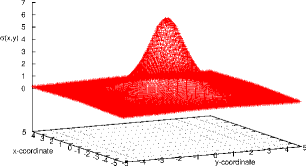
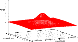
Figure 1: Induced surface charge density at the perfect conductor plane for Na⁺ ion placed at 1.5 Å (Upper panel) and 2.0 Å (Lower panel) away from the perfect conductor. The size of the surface unit cell is 10 Å x 10 Å and the height of the supercell is 20 Å.

The behaviour of the induced surface electron density, $\sigma_{ind}({\bf R})$, at two different distances of the Na⁺ ion from the perfect conductor plane is shown in Fig. 1, for a supercell with transversal area $A=100$ Ų and a height L of 20 Å. It is evident that the induced electron density becomes laterally more extended as the ion separates from the surface but the net total charge remains constant and is equal to $-e$. In other words, the contributions from plane-wave coefficients $\sigma({\bf G}\neq 0)$ decrease with the distance and $\sigma_{ind}({\bf R})$ becomes practically uniform when this distance is sufficiently large.

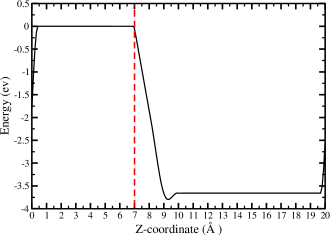
Figure 2: Laterally averaged electrostatic potential, $\bar{\phi}(z)=\bar{\phi}_{s}(z)+\bar{\phi}_{m}(z)+\phi_{dip}(z)+\phi_{1}$, as a function of the $z$ coordinate for a Na⁺ ion placed 2 Å away from the perfect conductor plane located at $z=7$ Å. The dipole layer is located at $z$ = 20 Å. Same supercell as in Fig. 1.

The characteristic behaviour of the laterally averaged, dipole-corrected electrostatic potential, $\bar{\phi}(z)=\bar{\phi}_{s}(z)+\bar{\phi}_{ind}(z)+\phi_{dip}(z)+\phi_{1}$, is illustrated in Fig. 2 as a function of the $z$ coordinate when the Na⁺ ion is placed 2 Å outside the perfect conductor plane located at $z=7$ Å. Again, the supercell is the same as in Fig. 1. The potential is constant and equal to zero inside the perfect conductor as dictated by the condition in Eqn.(55). The discontinuous change in slope at the perfect conductor plane (located at $z=7$Å) is induced by the laterally averaged surface charge density $\bar{\sigma}$. In the region between the perfect conductor plane and the ion (placed at $z=9$Å), the slope is constant corresponding to a constant electric field. The spatial extension of the charge distribution of the ion is reflected by the deviation from this linear behaviour. The calculated value of the slope in the potential in this region is 1.81 eV/Å, which is precisely the value of $4\pi\bar{\sigma}/\epsilon_{0}$ = 1.81 eV/Å for the z-component of the electrical field inside a capacitor with plates having opposite surface charge densities of $\bar{\sigma}=e/A=0.01$ eÅ^-2, since $A=100$ Ų. At the dipole layer located at $z=$ 20 Å the potential makes a jump, so that the potential is periodic across the supercell boundaries at $z=0$ and 20 Å. Note that the representation of the surface charge on a single plane of grid points give rise to a well-behaved electrostatic potential in contrast to the dipole layer, which has to be smeared out in the $z$ direction in order to damp out Gibbs oscillations.

To facilitate the discussion of the behaviour of the calculated interaction energy, $E_{int}$, between the Na⁺ ion and the PC as defined in Eqn.(11), we have decomposed this energy into the contributions $\bar{E}_{int}$ and $E_{int}^{\prime}$ from the laterally averaged, $\bar{\sigma}_{ind}$, and the laterally varying surface charge density, $\sigma_{ind}^{\prime}({\bf R})$, respectively. Note that $E_{s}[n_{s0}$] in Eqn.(11) has been obtained for the ion in the supercell with a uniform neutralising background. The two contributions $\bar{E}_{int}$ and $E_{int}^{\prime}$ are shown in Figs. 3 and 4 for different surface areas of the supercell. Since we shall compare DFT results for the Na⁺ with the analytical results for a point charge in Eqns.(73) and (76), we need to avoid a significant overlap between the electron density of the ion and the induced electron density at the perfect conductor plane. With this, we shall only consider distances of the Na⁺ from the perfect conductor plane larger than 0.8 Å.

As shown in Fig. 3 (Upper panel), the contribution from the uniform surface charge distribution results in a linear variation of the interaction energy with the ion distance to the PC surface. This linear behaviour and the decrease in magnitude of the associated force (given by the negative gradient) with increasing transversal area is in agreement with the corresponding result of Eqn.(73) in the point charge model. The relative difference between the latter result and the computed interaction energy is smaller than the 2%, as shown in Fig. 3 (Lower panel). These small differences can in part be attributed to the polarisation of the semi-core of the Na⁺and at shorter distances in part the spatial extension of the charge distribution of the ion. Note that $\bar{E}_{int}$ for the different $A$ do not cross at the perfect conductor plane but at a distance of about 1.75 Å outside the perfect conductor plane due to the extra energy term of Eqn.(75). In fact this term gives that the crossing is located at $L/12$, which is in excellent agreement with the result in Fig. 3 (Upper panel).

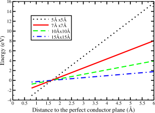
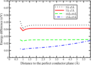
Figure 3: (Upper panel) Calculated contribution, $\bar{E}_{int}$, to the interaction energy from the laterally averaged part of the induced surface charge density, $\bar{\sigma}$, as a function of the distance to the perfect conductor plane for the different sizes of the surface unit cell. (Lower panel) Calculated energy difference with respect to the point charge case result of Eqn.(73). The height of the supercell is 20 Å.

In contrast to the laterally average interaction energy $\bar{E}_{int}$, the contribution to the interaction energy from the laterally varying part $E_{int}^{\prime}$ is always attractive, becomes more dominant with increasing surface area and decay rapidly with the distances from the perfect conductor, as shown in Fig. 4 (Upper panel). This result is in close agreement with the result in Eqn.(76), obtained from the corresponding contribution in the point charge model, as shown by the difference between these two results in Fig. 4 (Lower panel). In fact, relative energy differences between DFT and the point charge case are smaller than 2%. In the limit of infinite surface area, the interaction tends to the classical image interaction.

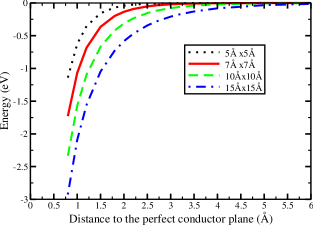
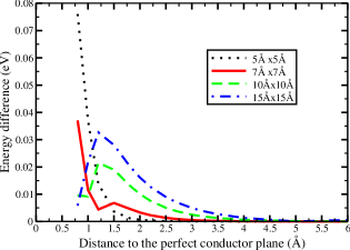
Figure 4: (Upper panel) Calculated contribution, $E_{int}^{\prime}$, to the interaction energy from the laterally varying part of the induced surface charge density, $\sigma^{\prime}({\bf R})$, as a function of the distance of the ion to the perfect conductor plane for the different sizes of the surface unit cell.(Lower panel) Calculated energy difference with respect to the point charge model of Eqn.(76). The height of the supercell is 20 Å.

We now present the calculated Hellmann-Feynman force along the $z$ direction in Fig. 5. The force is always attractive and becomes constant for large distances of the ion from the perfect conductor plane. As the ion approaches to perfect conductor, the effect of the laterally varying components of the induced charge density become increasingly more important, thus leading to an increased attraction. Clearly, the magnitude of this attraction increases with the transversal area. In the limit of infinite surface area, the induced force will tend to the classical force exerted by the image charge. We observe that the differences with respect to the point charge case are smaller than 2.5%.

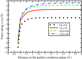
Figure 5: Calculated Hellman-Feynman force on the Na⁺ ion as a function the distance, $z_{0}$, from the perfect conductor plane for the different sizes of the surface unit cell. The height of the super cell is 20 Å. Differences with respect to the point charge case are lower than 2.5%.

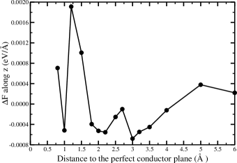
Figure 6: Test of the consistency between the Hellman-Feynman force on the ion and the force from the gradient of the total energy. $\Delta F$ is the difference between these two forces and values are smaller than the 0.06% of the computed forces. Same supercell as in Fig. 1.

Finally, as a critical test of the implementation of the perfect conductor model, we analyse the consistency between the computed Hellman-Feynman force on the ion and the gradient of the total energy. In Fig. 6, we show the difference between the force, $F_{z}$, computed along the $z$ direction using Eqn.(22) and the numerical derivative of the interaction energy, $-\partial E_{int}/\partial z_{0}$, as a function of the Na⁺ distance to the perfect conductor. Ideally, this difference should be zero but, due to numerical errors, small deviations are always expected. In fact, errors are essentially smaller than the 0.06% of the computed forces, showing that sufficient numerical consistency has been achieved. This level of self-consistency is also obtained for smaller distances where we have a more substantial overlap of the electron densities. Note that this high degree of consistency even in the case of overlapping electron densities is guaranteed by using the density response in Eqn.(59) that obeys the symmetry condition in Eqn.(8).

The above results suggest that we have derived and implemented a DFT method for a charged system in front of a perfect conductor. Small differences with respect to the the point charge case could be attributed to the differences in the spatial extension of the densities of charge and that the point charge model does not include any polarisation, which will be inevitably present when placing atoms or molecules under the electrical field generated by the induced potential.

We believe that the use of this new DFT methodology becomes particularly convenient since it allows to the possibility of computing DFT problems of different charge states in a controllable way, that is, by defining (at will) the amount of charge transfer between the system and the perfect conducting plane. However, we have shown that the use of the perfect conductor approximation only induces attractive interactions, which would make the system to move closer and closer to the perfect conductor plane. This represent a limitation if one aims to make use of this DFT methodology to simulate realistic problems involving metallic surfaces. In fact, the metallic surface will exert repulsive forces for sufficiently close distances, thus avoiding the system to collapse with the surface [26]. This lack of repulsion is a direct consequence of having considered only the electrostatic interactions in the approximate energy functional of Eqn.(1). In a following publication [27], we propose a new procedure to surmount this limitation.

5 Concluding Remarks

To the final purpose of developing a simplified density functional theory (DFT) method for treating charged atoms and molecules on an ultrathin-insulating film supported by a metal substrate, we have presented a new approximate DFT methodology for the calculation of the total energy, ionic (Hellman-Feynman) forces and electronic structure of a charged system placed in front of a metal surface. In this new methodology, the electron densities of the metal surface and the charged system are assumed to be non-overlapping and there is only an electrostatic interaction between these two fragments. Whereas the charged system is treated fully using DFT, the metal surface is approximated within linear response, corresponding to an expansion of the energy of the metal surface to second order in the electrostatic potential from the charged system. In particular, we have carried out a careful analysis of the effect of periodic boundary conditions and derived appropriate dipole corrections for the total energy and the ionic forces. The proposed method have two main advantages. First, the metal electron states are not treated explicitly but only implicitly through their density response to an external electrostatic field, which can be captured in a simple model. Here, we have explicitly considered the perfect conductor approximation for the metal response although the method is not strictly limited to this approximation. In the perfect conductor model the screening length by the conduction electron is assumed to be zero and the screening charge resides on a plane. Second, different charge states of the charged system can be handled directly. Based on the simple perfect conductor approximation for the metal response, we have implemented this method in the density functional theory VASP code.

A simple illustration and test of this method is provided by the case of the Na⁺ ion outside a perfect conductor. The six electrons in the $p$ semi-core of the ion were included in the calculations. The success of our implementation is demonstrated by the excellent agreement between the calculated Hellman-Feynman force and the gradient of the interaction energy, even in the region close to the perfect conductor plane where the electron density of the ion overlaps with the induced charge density at the perfect conductor plane. Furthermore, the small polarisability of the ion makes the calculated interaction energy to be in close agreement to the analytical result for a point charge outside the perfect conductor within a supercell of finite size.

Finally, to fulfil our overall aim, we need to include the missing interactions in our simplified scheme arising from over-lapping densities and van der Waals interactions between the ultrathin-insulating film with charged adsorbates and the metal substrate. We plan to do this by developing a simple parametrised force field between the metal substrate and the atoms in the adjacent layer of the film, where the parameters are obtained by fitting the resulting interactions to DFT calculations of the film (without adsorbates) over the metal substrate. The presentation of this scheme and associated results of this model are deferred to a separate publication.

References

References

- [1] J. Repp, G. Meyer, F. E. Olsson, M. Persson, Science 305, 493 (2004).
- [2] F. E. Olsson, S. Paavilainen, M. Persson, J. Repp, G. Meyer, Phys. Rev. Lett. 98, 176803 (2007).
- [3] J. Repp, G. Meyer, S. M. Stojković, A. Gourdon, C. Joachim, Phys. Rev. Lett. 94, 026803 (2005).
- [4] J. Repp, G. Meyer, S. Paavilainen, F. E. Olsson, M. Persson, Science 312, 1196 (2006).
- [5] J. Repp, P. Liljeroth, G. Meyer, Nature Phys. 4, 975 (2010).
- [6] P. Liljeroth, J. Repp, and G. Meyer, Science 317, 1203 (2007).
- [7] F. Mohn, J. Repp, L. Gross, G. Meyer, M. S. Dyer, and M. Persson, Phys. Rev. Letter 105, 266102 (2010).
- [8] P. Hohenberg and W. Kohn, Phys. Rev., 136, B-864, (1964).
- [9] W. Kohn and L. J. Sham, Phys. Rev., 140, 1133A, (1965).
- [10] Cohen AJ, Mori-Sánchez P and Yang W, Science, 321 (5890): 792-794 (2008)
- [11] V. I. Anisimov, J. Zaanen, and O. K. Andersen, Phys. Rev. B 44, 943 (1991); V. I. Anisimov, I. V. Solovyev, M. A. Korotin, M. T. Czyzyk, and G. A. Sawatzky, ibid. 48, 16929 (1993).
- [12] M. Cococcioni and S. deGironcoli, Phys. Rev. B 71, 035105 (2005).
- [13] Sit, P. H.-L.; Cococcioni, M.; Marzari, N. J. Electroanal. Chem. 607, 107 (2007).
- [14] J. Repp, G. Meyer, S. Paavilainen, F. E. Olsson, and M. Persson, Physical Review Letters 95, 225503 (2005).
- [15] N. W. Ashcroft and N. D. Mermin, Solid State Physics, (Holt and Rinehart and Winston, 1977).
- [16] C. Kittel, Introduction to Solid State Physics, Seventh Edition, (JOHN WILEY & SONS, 2005).
- [17] J. Neugebauer and M. Scheffler, Phys. Rev. B 46, 16067 (1992).
- [18] L. Bengtsson, Phys. Rev. B 59, 12301 (1999).
- [19] N. D. Lang and W. Kohn, Phys. Rev. B 1, 4555 (1970); Phys. Rev. B 3, 1215 (1971); Phys. Rev. B 7, 3541 (1973)
- [20] A. Liebsch, Electronic Excitations at Metal Surfaces, (Plenum Press, NY and London), (1997)
- [21] See p. 32 in Ref. [20]
- [22] See Fig. 2.8 in Ref. [20]
- [23] G. Kresse, J. Furthmuller, Phys. Rev. B 54, 11169 (1996); G. Kresse, D. Joubert, Phys. Rev. B 59, 1758 (1999).
- [24] P.E. Blöchl, Phys. Rev. B 50, 17953, (1994).
- [25] J. P. Perdew, K. Burke, and M. Ernzerhof, Phys. Rev. Lett. 77, 3865 (1996).
- [26] The origin of this repulsive interaction is purely due to Pauli’s forces, which arise from the overlapping of the system and the metal electronic clouds.
- [27] Scivetti I. and Persson M. (in preparation).