The Zagier polynomials. Part II: Arithmetic properties of coefficients

Abstract.

The modified Bernoulli numbers

$$B_{n}^{*}=\sum_{r=0}^{n}\binom{n+r}{2r}\frac{B_{r}}{n+r},\quad n>0$$

introduced by D. Zagier in $1998$ were recently extended to the polynomial case by replacing $B_{r}$ by the Bernoulli polynomials $B_{r}(x)$. Arithmetic properties of the coefficients of these polynomials are established. In particular, the $2$-adic valuation of the modified Bernoulli numbers is determined. A variety of analytic, umbral, and asymptotic methods is used to analyze these polynomials.

1. Introduction

The Bernoulli numbers $B_{n}$, defined by the generating function

(1.1) $$\frac{t}{e^{t}-1}=\sum_{n=0}^{\infty}B_{n}\frac{t^{n}}{n!},$$

were extended by D. Zagier [17] with the introduction of the so-called modified Bernoulli numbers $B_{n}^{*}$ defined by

(1.2) $$B_{n}^{*}=\sum_{r=0}^{n}\binom{n+r}{2r}\frac{B_{r}}{n+r}.$$

Note that $B_{0}^{*}$ is undefined. Arithmetic properties of $B_{2n}$ ($B_{1}=-\tfrac{1}{2}$ and $B_{2n+1}=0$, for $n>0$), include the von Staudt–Clausen theorem which states that, for $n>0$,

(1.3) $$B_{2n}\equiv-\sum_{\genfrac{}{}{0.0pt}{}{(p-1)|2n}{\text{$p$ prime}}}\frac{1}{p}\quad\bmod 1.$$

It follows that the denominator of $B_{2n}$ is the product of all primes $p$ such that $p-1$ divides $2n$. On the other hand, the numerators of $B_{2n}$ are still a mysterious sequence.

The definition (1.2) shows that $B_{n}^{*}$ is a rational number. Write it in reduced form and define

(1.4) $$\alpha_{n}=\operatorname{denom}(B_{n}^{*}).$$

Zagier [17] showed that

(1.5) $$\tilde{B}_{n}=2nB_{n}^{*}-B_{n}$$

satisfies

(1.6) $$\tilde{B}_{n}\equiv\sum_{\genfrac{}{}{0.0pt}{}{(p+1)|n}{p\text{ prime }}}\frac{1}{p}\quad\bmod 1,\quad(n>0,\,n\text{ even})$$

that implies

(1.7) $$2nB_{n}^{*}\equiv-\sum_{\genfrac{}{}{0.0pt}{}{(p-1)|n}{p\text{ prime }}}\frac{1}{p}+\sum_{\genfrac{}{}{0.0pt}{}{(p+1)|n}{p\text{ prime }}}\frac{1}{p}\quad\bmod 1,\quad(n>0).$$

This statement shows that if $p$ is a prime dividing $\alpha_{n}$ (defined in (1.4)), then at least one of $p$, $p-1$ and $p+1$ divides $n$. In particular, all prime factors $p$ of $\alpha_{n}$ satisfy $p\leq n+1$. In fact, from computing the first $1000$ terms, it appears that, conjecturally, the following stronger statement is true: if $p$ is a prime dividing $\alpha_{n}$, then $p+1$ or $p-1$ divides $n$.

The first few values of the sequence $\{B_{n}^{*}\}$ are

$$\frac{3}{4},\frac{1}{24},-\frac{1}{4},-\frac{27}{80},-\frac{1}{4},-\frac{29}{1260},\frac{1}{4},\frac{451}{1120},\frac{1}{4},-\frac{65}{264},\ldots$$

Our particular interest will be in the $2$-adic properties of this sequence and the $2$-adic valuation of $B_{n}^{*}$ will be worked out completely. A guiding question motivated by the first few terms as above is:

Question 1.1.

Is the denominator $\alpha_{n}$ always divisible by $4$?

This basic question will become particularly relevant when considering the corresponding modifications of Bernoulli polynomials. This is addressed at the end of this introduction.

It turns out that $\alpha_{2n+1}=4$, so only even indices need to be considered. The first few values of $\tfrac{1}{4}\alpha_{2n}$ are given by

(1.8) $$6,\,20,\,315,\,280,\,66,\,3003,\,78,\,9520,\,305235,\,20900,\,138,\,19734,\,6,\,7540,\ldots$$

This sequence has been recently added to OEIS (the database created by N. Sloane) as entry $\text{A}216912$. The next figure shows the $2$-adic valuation of $\alpha_{2n}$; that is, the highest power of $2$ that divides $\alpha_{2n}$.

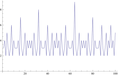
Figure 1. Power of $2$ that divides denominator of $B_{2n}^{*}$

Symbolic computations lead us to discover the next result. In particular, this answers Question 1.1 in the affirmative.

Theorem 1.2.

For $n>0$,

$$\nu_{2}(\alpha_{n})=-\nu_{2}(B^{*}_{n})=2+\nu_{2}(n)-\begin{cases}1&\text{if $n\equiv 6\bmod 12$},\\ 2&\text{if $n\equiv 0\bmod 12$},\\ 0&\text{otherwise.}\end{cases}$$

In particular, $B_{n}^{*}$, the denominator of $\alpha_{n}$, is divisible by $4$.

Note that this may be rephrased in the following way: The $2$-adic valuations $\nu_{2}(8nB^{*}_{2n})$ form a periodic sequence of period $6$ with values

(1.9) $$\left\{0,\,0,\,1,\,0,\,0,\,2\right\}.$$

This is an unexpected variation on the period $6$ theme: D. Zagier proved that the sequence $\{B_{2n+1}^{*}\}$ is $6$-periodic.

The modified Bernoulli numbers $B_{n}^{*}$ were extended in [6] to the Zagier polynomials defined by

(1.10) $$B_{n}^{*}(x)=\sum_{r=0}^{n}\binom{n+r}{2r}\frac{B_{r}(x)}{n+r},$$

so that $B_{n}^{*}=B_{n}^{*}(0)$. The first few are:

$$\frac{1}{4}(2x+3),\frac{1}{24}\left(6x^{2}+18x+1\right),\frac{1}{12}(2x+3)\left(x^{2}+3x-1\right),$$

$$\quad\frac{1}{80}\left(10x^{4}+60x^{3}+90x^{2}-27\right),\frac{1}{60}(2x+3)\left(3x^{4}+18x^{3}+23x^{2}-12x-5\right),\ldots$$

In analogy to $\alpha_{n}$ in (1.4), define, for $j\in\mathbb{Z}$,

(1.11) $$\alpha_{n,j}=\operatorname{denom}(B_{n}^{*}(j)).$$

It is shown in Lemma 3.2 of Section 3 that, under the assumption that $4$ divides $\alpha_{n}$, the denominators $\alpha_{n,j}$ equal $\alpha_{n}$ for any $j\in\mathbb{Z}$. Combining this with Theorem 1.2, one obtains:

Theorem 1.3.

The denominator $\alpha_{n,j}=\operatorname{denom}(B_{n}^{*}(j))$ does not depend on the value $j\in\mathbb{Z}$.

Special values of $B_{n}^{*}(x)$ present interesting arithmetic properties. The relation

(1.12) $$B_{n}^{*}(x+1)=B_{n}^{*}(x)+\frac{1}{2}U_{n-1}\left(\frac{x}{2}+1\right),$$

relating $B_{n}^{*}$ to the Chebyshev polynomial of the second kind, appears as Lemma $10.2$ in [6]. In particular, this shows the identity

(1.13) $$B_{n}^{*}(1)=B_{n}^{*}+\frac{n}{2}.$$

On the other hand, the values $B_{n}^{*}(-1)$ are connected to the asymptotic expansion of the function

(1.14) $$V(z)=\log z+\psi\left(z+\frac{1}{z}\right)$$

at $z\to 0$. Here, $\psi(z)$ is the digamma function

(1.15) $$\psi(z)=\frac{\Gamma^{\prime}(z)}{\Gamma(z)},$$

the logarithmic derivative of the gamma function. The proof of the next statement appears in Section 7.

Theorem 1.4.

Define the numbers $v_{n}$ by the asymptotic expansion

(1.16) $$V(z)\sim\sum_{n=0}^{\infty}v_{n}z^{n}.$$

Then $v_{n}=-2B_{n}^{*}(-1)$.

The value $v_{2n-1}=(-1)^{n}/2$ is simple to obtain, but

(1.17) $$v_{2n}=(-1)^{n+1}\left[\frac{1}{n}+\sum_{k=1}^{n}(-1)^{k}\binom{n+k-1}{n-k}\frac{B_{2k}}{2k}\right]$$

requires further work.

A second motivation for considering the sequence $\{v_{n}\}$ comes from the natural interest in the sequence $\{B_{2n}^{*}\}$. The established fact that $\{B_{2n+1}^{*}\}$ is $6$-periodic has no obvious analog for the even indices. It turns out that the function $V(z)$ satisfies

(1.18) $$\sum_{n=1}^{\infty}B_{2n}^{*}z^{2n}=-\frac{1}{2}V(z)-\frac{z}{4}\left[\frac{1}{z^{2}+1}+\frac{2(1-z^{4})}{1-z^{6}}\right],$$

thus connecting $B_{2n}^{*}$ and $v_{n}$.

A variety of expressions for the coefficients $v_{n}$ are provided. Section 6 gives one using the umbral method and Section 7 exploits a relation between the Zagier polynomials $B_{n}^{*}$ and the Chebyshev polynomials $U_{n}(x)$ to determine $v_{n}$. A direct asymptotic method is used in Section 8 and Section 9 presents a family of polynomials that determine $v_{n}$. The classical integral representation of the digamma function is used in Section 10, the formula of Faà di Bruno to differentiate compositions is used in Section 11 and, finally, a recurrence for $v_{n}$ is analyzed in Section 12 by the WZ-method [14].

2. The $2$-adic valuation of $B^{*}_{n}$

The goal of this section is to establish Theorem 1.2 which determines the $2$-adic valuation of the sequence $B^{*}_{n}$.

The strategy employed here is as follows. It is a consequence of the von Staudt–Clausen congruence that the Bernoulli numbers $2B_{n}$ are $2$-integral. From this one may conclude that the rational numbers $4nB^{*}_{n}$ are $2$-integral as well. In particular, these numbers can be reduced modulo powers of $2$ to determine their $2$-adic valuation. Here, it will be sufficient to reduce them modulo $8$. To begin with, the classical Bernoulli numbers are reduced modulo $8$.

Proposition 2.1.

The following congruences hold modulo $8$:

$$2B_{0}\equiv 2,\hskip 10.00002pt2B_{2}\equiv 3,\hskip 10.00002pt2B_{2k}\equiv\left\{\begin{array}[]{ll}1&\text{if $k$ even},\\ 5&\text{if $k$ odd},\end{array}\right.$$

with $k>1$.

Proof.

The von Staudt–Clausen theorem states that

(2.1) $$pB_{2k}\equiv p-1\bmod p^{\ell+1}$$

for $p$ prime, $k\geq 2$ and when $(p-1)p^{\ell}$ divides $2k$; see [13], formula $24.10.2$ on page 593. Now take $p=2$ and $\ell=1$. Then for $k\geq 2$ it follows that $2B_{2k}\equiv 1\bmod 4$. Therefore $2B_{2k}\equiv 1\text{ or }5\bmod 8$. In the case $k$ is even, one may take $\ell=2$, since then $(p-1)p^{\ell}=4$ divides $2k$. Therefore

(2.2) $$2B_{2k}\equiv 1\bmod 8.$$

A different proof of this fact appears in [4]. The identity established there is

(2.3) $$2B_{2k}\equiv 1\bmod 2^{r+1}$$

where $2^{r}$ is the highest power of $2$ that divides $2k$. In particular, for $k$ even, $r\geq 2$ and the result follows.

The case $k$ odd requires a different approach.

Let $U_{m}$ be the numerator and $V_{m}$ the denominator of $B_{m}$, so that $B_{m}=U_{m}/V_{m}$ and $(U_{m},V_{m})=1$, $V_{m}>0$. Voronoi’s congruence [11, Proposition 15.2.3] states that, if $m\geq 2$ is even and $a$, $n$ are positive integers with $(a,n)=1$, then

$$(a^{m}-1)U_{m}\equiv ma^{m-1}V_{m}\sum_{j=1}^{n-1}j^{m-1}\left[\frac{ja}{n}\right]\hskip 10.00002pt\bmod n.$$

As usual, $[x]$ refers to the greatest integer less than or equal to $x$. It follows from the von Staudt–Clausen congruence that $2B_{2m}$ has $2$-adic valuation $0$ for $m>0$, so that they are $2$-integral. Voronoi’s congruence with $a=3$ and $n=64$ therefore yields

$$(3^{m}-1)2B_{m} \equiv 2m\,3^{m-1}\sum_{j=1}^{63}j^{m-1}\left[\frac{3j}{64}\right]\hskip 10.00002pt\bmod 64.$$

One easily checks that, for even $m$, $3^{m}-1\equiv 4m$ modulo $64$. Similarly, after checking finitely many cases, for $m\equiv 2$ modulo $4$ with $m\geq 6$,

$$3^{m-1}\sum_{j=1}^{63}j^{m-1}\left[\frac{3j}{64}\right]\equiv 42\bmod 64.$$

Combining these, one finds, for $m\equiv 2$ modulo $4$ with $m\geq 6$,

$$2B_{m}\frac{m}{2} \equiv 5\frac{m}{2}\hskip 10.00002pt\bmod 8.$$

Hence, if $m=2k$ with $k\geq 3$ odd, then $2B_{m}\equiv 5$ modulo $8$. ∎

Further basic ingredients are the following generating functions.

Proposition 2.2.

The following generating functions admit rational closed-forms:

(2.4) $$2+\sum_{n=1}^{\infty}x^{n}\sum_{k=0}^{n}\binom{n+k}{2k}\frac{2n}{n+k} =\frac{2-3x}{1-3x+x^{2}},$$

$$2+\sum_{n=1}^{\infty}x^{n}\sum_{k=0}^{\left\lfloor n/2\right\rfloor}\binom{n+2k}{4k}\frac{2n}{n+2k} =\frac{\left(1-2x\right)\left(2-2x+x^{2}\right)}{\left(1-x+x^{2}\right)\left(1-3x+x^{2}\right)},$$

$$2+\sum_{n=1}^{\infty}x^{n}\sum_{k=0}^{\left\lfloor n/2\right\rfloor}\left(-1\right)^{k}\binom{n+2k}{4k}\frac{2n}{n+2k} =\frac{2-6x+7x^{2}-2x^{3}}{1-4x+7x^{2}-4x^{3}+x^{4}}.$$

Proof.

These readily follow from the generating function for $T_{n}(x)$, the Chebyshev polynomials of the first kind, given by

(2.5) $$\sum_{n=0}^{\infty}T_{n}(x)t^{n}=\frac{1-xt}{1-2xt+t^{2}}$$

and from the fact

(2.6) $$\sum_{r=0}^{n}\binom{n+r}{2r}\frac{x^{r}}{n+r}=\frac{1}{n}T_{n}\left(\frac{x}{2}+1\right)$$

proved as Lemma $9.1$ in [6]. ∎

Equipped as such, a proof of Theorem 1.2 is given next. The statement of this theorem is repeated for the convenience of the reader.

Theorem 2.3.

For $n>0$,

$$-\nu_{2}(B^{*}_{n})=2+\nu_{2}(n)-\begin{cases}1&\text{if $n\equiv 6\bmod 12$},\\ 2&\text{if $n\equiv 0\bmod 12$},\\ 0&\text{otherwise}.\end{cases}$$

Proof.

It is convenient to remark at the beginning that the case of odd $n$ is simple and is a consequence of Zagier’s result on the periodicity of the sequence $B^{*}_{2n+1}$.

Working modulo $8$ and using Proposition 2.1, it follows that $2B_{0}\equiv 2$, $2B_{1}\equiv-1$, $2B_{2}\equiv 3$ and for $k>1$,

$$2B_{2k}\equiv 3-2\left(-1\right)^{k}.$$

Note that $\binom{n+k}{2k}\frac{2n}{n+k}$ is an integer. Thus it follows from (1.2) that $4nB^{*}_{n}$ is a $2$-adic integer. For $n\geq 1$, these numbers reduce modulo $8$ to

$$4nB_{n}^{\ast} =\sum_{k=0}^{\left\lfloor n/2\right\rfloor}\binom{n+k}{2k}\frac{2n}{n+k}2B_{k}$$

$$=-n^{2}+\sum_{k=0}^{\left\lfloor n/2\right\rfloor}\binom{n+2k}{4k}\frac{2n}{n+2k}2B_{2k}$$

$$\equiv-n^{2}+2-n\binom{n+1}{3}+\sum_{k=0}^{\left\lfloor n/2\right\rfloor}\left[3-2\left(-1\right)^{k}\right]\binom{n+2k}{4k}\frac{2n}{n+2k},$$

where in the second equality, the $-n^{2}$ term comes from the contribution of $B_{1}=-1/2$, the only nonzero Bernoulli number of odd index. Also, for the final congruence, adjusting for the $k=0$ and $k=1$ cases in which $2B_{0}=2$ and $2B_{2}=1/3\equiv 3$ respectively, produces the extra terms

$$\binom{n}{0}\frac{2n}{n}\left(2B_{0}-1\right)+\binom{n+2}{4}\frac{2n}{n+2}\left(2B_{2}-5\right)\equiv 2-n\binom{n+1}{3}.$$

Using Proposition 2.2 modulo $8$ now gives

$$4+\sum_{n=1}^{\infty}4nB_{n}^{\ast}x^{n} \equiv\frac{2}{1-x}-\frac{x\left(1+x\right)\left(1+x^{2}\right)}{\left(1-x\right)^{5}}+3\frac{\left(1-2x\right)\left(2-2x+x^{2}\right)}{\left(1-x+x^{2}\right)\left(1-3x+x^{2}\right)}$$

$$\quad-2\frac{2-6x+7x^{2}-2x^{3}}{1-4x+7x^{2}-4x^{3}+x^{4}},$$

where it is readily verified that the right-hand side is a rational function whose coefficients modulo $8$ are periodic with period $24$. The even part simplifies to

$$\sum_{n=1}^{\infty}8nB_{2n}^{\ast}x^{2n}\equiv\frac{x\left(3+x+6x^{2}+x^{3}+3x^{4}+4x^{5}\right)}{1-x^{6}}.$$

This implies

$$\nu_{2}\left(8nB_{2n}^{\ast}\right)=\left\{\begin{array}[]{ll}0&\text{if $(n,3)=1,$}\\ 1&\text{if $n\equiv 3\hskip 10.00002pt\bmod 6,$}\\ 2&\text{if $n\equiv 0\hskip 10.00002pt\bmod 6,$}\end{array}\right.$$

which proves the claim. ∎

3. The denominators of $B_{n}^{*}(j)$

The goal of this section is to establish Theorem 1.3. It states that the denominator of $B^{*}_{n}(j)$ does not depend on $j\in\mathbb{Z}$. The proof begins with the identity

(3.1) $$B_{n}^{*}(x+1)=B_{n}^{*}(x)+\frac{1}{2}U_{n-1}\left(\frac{x}{2}+1\right),$$

appearing as Lemma $10.2$ in [6] which establishes a relation between the Zagier polynomials and the Chebyshev polynomials of the second kind $U_{n}(x)$.

Lemma 3.1.

For every half-integer $x$, the numbers $U_{n}(x)$ are integers.

Proof.

This is clear upon using the determinant representation

(3.6) $$U_{n}(x)=\left|\begin{array}[]{cccc}2x&1&&0\\ 1&2x&\ddots&\\ &\ddots&\ddots&1\\ 0&&1&2x\end{array}\right|$$

for the Chebyshev polynomial. To verify (3.6) denote the determinant by $D_{n}(x)$. By expansion by minors, it follows that $D_{n+1}(x)=2xD_{n}(x)-D_{n-1}(x)$. The same recurrence is satisfied by $U_{n}(x)$ and a direct computation gives $D_{n}(x)=U_{n}(x)$ for $n=1,\,2$. Thus, $U_{n}(x)=D_{n}(x)$ for all $n\in\mathbb{N}$.

An alternative proof employs the generating function of the $U_{n}(x)$ polynomials

(3.7) $$\sum_{k\geq 0}U_{k}(x)t^{k}=\frac{1}{1-2xt+t^{2}}.$$

Choosing $x=\frac{p}{2}$ with $p$ integer, it follows that

(3.8) $$\sum_{m\geq 0}U_{m}\left(\frac{p}{2}\right)t^{m}=\frac{1}{1-pt+t^{2}}=\frac{1}{1-t(p-t)}=\sum_{k\geq 0}t^{k}(p-t)^{k}$$

since by choosing $t$ small enough, $|t(p-t)|<1$. The coefficient of $t^{m}$ in this sum, which is $U_{m}\left(\frac{p}{2}\right)$, is clearly an integer. ∎

Lemma 3.2.

The denominator of $B^{*}_{n}(j)$ is independent of $j\in\mathbb{Z}$. In other words, for all $j\in\mathbb{Z}$,

(3.9) $$\operatorname{denom}B^{*}_{n}(j)=\operatorname{denom}B^{*}_{n}.$$

Proof.

Assume $j>0$. It is a consequence of Theorem 1.2 that the denominator of $B_{n}^{*}$ is divisible by $4$, and thus is $4t$ for some $t\in\mathbb{Z}$.

Assume, therefore, by induction that the denominator of $B_{n}^{*}(j)$ is $4t$ as well; that is, in reduced form

(3.10) $$B_{n}^{*}(j)=\frac{x}{4t},$$

with $x=x(j)$ an odd integer. The identity (3.1) coupled with Lemma 3.2 gives

(3.11) $$B_{n}^{*}(j+1)=\frac{x}{4t}+\frac{w}{2}=\frac{x+2wt}{4t},$$

with $w\in\mathbb{Z}$. The last fraction in (3.11) is also in reduced form. Indeed, the numerator is odd so there is no cancellation of the factor $4$ and if $p$ is an odd prime that divides both $x+2wt$ and $4t$, then it divides $\gcd(x,t)=1$. Therefore $B_{n}^{*}(j+1)$ also has denominator $4t$, the denominator of $B_{n}^{*}$. This proof easily adapts to the case when $j$ is negative. ∎

4. An asymptotic expansion related to the numbers $B^{*}_{n}$

The generating function

$$\sum_{n=1}^{\infty}B^{*}_{n}(x)z^{n}=-\frac{1}{2}\log z-\frac{1}{2}\psi\left(z+1/z-1-x\right)$$

appears as Theorem 5.1 of [6]. Here $\psi(z)$ is the digamma function

(4.1) $$\psi(z)=\frac{\Gamma^{\prime}(z)}{\Gamma(z)},$$

the logarithmic derivative of the gamma function. The asymptotic expansion for the auxiliary function

(4.2) $$V(z)=\log z+\psi\left(z+\frac{1}{z}\right)$$

as $z\to 0$ in the form

(4.3) $$V(z)\sim\sum_{n=0}^{\infty}v_{n}z^{n}$$

will yield a relation between the numbers $B^{*}_{n}$ and the sequence $v_{n}$ in (4.3).

The value of $\alpha_{2n+1}$ has been established in [6].

Theorem 4.1.

For $j\in\mathbb{Z}$, the coefficients $4B_{2n+1}^{*}(j)$ are odd integers. This gives

(4.4) $$\alpha_{2n+1}=4.$$

The generating function for the much more involved case of $\alpha_{2n}$ is

$$\sum_{n=1}^{\infty}B_{2n}^{*}(j)z^{2n}=-\frac{1}{2}\log z-\frac{1}{4}\psi\left(z+\frac{1}{z}+2+j\right)-\frac{1}{4}\psi\left(z+\frac{1}{z}-1-j\right).$$

This was given in Corollary $5.3$ of [6] and can be converted to

$$\sum_{n=1}^{\infty}B_{2n}^{*}(j)z^{2n} = -\frac{1}{2}\log z-\frac{1}{2}\psi\left(z+\frac{1}{z}\right)$$

$$-\frac{1}{4}\sum_{r=0}^{j+1}\left[\frac{z}{z^{2}+rz+1}+\frac{z}{z^{2}-rz+1}\right]+\frac{z}{4(z^{2}+1)}$$

using

(4.5) $$\psi(u+k)=\psi(u)+\sum_{r=0}^{k-1}\frac{1}{u+r}.$$

Now use the function $V(z)$ defined in (4.2) to obtain

(4.6) $$\sum_{n=1}^{\infty}B_{2n}^{*}(0)z^{2n}=-\frac{1}{2}V(z)-\frac{z}{4}\left[\frac{1}{z^{2}+1}+\frac{2(1-z^{4})}{1-z^{6}}\right].$$

This identity shows that Question 1.1 is indeed equivalent to the rational numbers $v_{2n}$ having even denominators.

A direct symbolic computation gives the values of the first few $v_{n}$ as

(4.7) $$\left\{0,\,-\frac{1}{2},\,\frac{11}{12},\,\frac{1}{2},\,-\frac{13}{40},\,-\frac{1}{2},\,\frac{29}{630},\,\frac{1}{2},\,\frac{109}{560},\,-\frac{1}{2},-\frac{67}{132},\,\frac{1}{2},\,\frac{6571}{6006}\right\}.$$

This data suggests that $|v_{n}|=1/2$ for $n$ odd but no simple pattern is observed for $n$ even.

5. The use of bounds on $\psi(z)$

The first approach to the computation of the coefficients $v_{n}$ is to use bounds for the digamma function $\psi(z)$ and its derivatives that exist in the literature. This process succeeds only for small values of $n$.

Proposition 5.1.

The function $V(z)$ satisfies

(5.1) $$\lim\limits_{z\to 0^{+}}V(z)=0,$$

that is, $v_{0}=0$.

Proof.

The inequality

(5.2) $$\frac{1}{2z}<\log z-\psi(z)<\frac{1}{z}$$

was established by H. Alzer [2]. This gives

(5.3) $$\log(z^{2}+1)-\frac{z}{z^{2}+1}<V(z)<\log(z^{2}+1)-\frac{z}{2(z^{2}+1)}$$

and the result follows from here. The inequality (5.2) has been improved by F. Qi and B. Guo [10] to

(5.4) $$\log\left(z+\frac{1}{2}\right)-\frac{1}{z}<\psi(z)<\log\left(z+e^{-\gamma}\right)-\frac{1}{z}.$$

∎

The next statement shows the computation of $v_{1}$. It requires sharper bounds on the derivative $\psi^{\prime}(x)$. The proof presented below should be seen as a sign that a different procedure is desirable for the evaluation of general $v_{n}$.

Proposition 5.2.

The function $V(z)$ satisfies

(5.5) $$\lim\limits_{z\to 0^{+}}V^{\prime}(z)=-\frac{1}{2},$$

that is, $v_{1}=-1/2$.

Proof.

The inequalities

(5.6) $$\frac{(k-1)!}{z^{k}}+\frac{k!}{2z^{k+1}}<(-1)^{k+1}\psi^{(k)}(z)<\frac{(k-1)!}{z^{k}}+\frac{k!}{z^{k+1}},\quad\text{ for }z>0,$$

are established in [8]. In the special case $k=1$ they produce

(5.7) $$\frac{1}{z}+\frac{1}{2z^{2}}<\psi^{\prime}(z)<\frac{1}{z}+\frac{1}{z^{2}}.$$

It turns out that the lower bound gives a sharp result for $V^{\prime}(z)$ as $z\to 0^{+}$. Indeed,

(5.8) $$V^{\prime}(z)=\left(1-\frac{1}{z^{2}}\right)\psi^{\prime}\left(z+\frac{1}{z}\right)+\frac{1}{z}<\frac{4z^{3}+z^{2}+4z-1}{2(1+z^{2})^{2}}.$$

The reader should check that the upper bound does not give useful information. Instead the inequality

(5.9) $$\psi^{\prime}(z)<e^{1/z}-1,$$

established in [9], is used to produce

(5.10) $$V^{\prime}(z)>\left(\frac{z^{2}-1}{z^{2}}\right)\left[\text{exp}\left(\frac{z}{z^{2}+1}\right)-1\right]+\frac{1}{z}.$$

The result now follows by letting $z\to 0$ in (5.8) and (5.10). ∎

The computation of $v_{n}$ by this procedure requires bounds on all derivatives of $\psi(x)$. The examples discussed above shows that this is not an efficient procedure. The next section presents an alternative.

6. The computation of $v_{n}$ by umbral calculus

The goal of this section is to compute the coefficients $v_{n}$ in the expansion (4.3) by the techniques of umbral calculus. The reader is referred to [6] for an introduction to these techniques and for the statements used in this section.

Introduce the auxiliary function

(6.1) $$F(x)=\psi\left(\frac{1}{x}\right)+\log x,$$

for $x>0$ and observe that

(6.2) $$V(z)=F\left(\frac{z}{z^{2}+1}\right)+\log(z^{2}+1).$$

Theorem 6.1.

The function $F(x)$ admits the asymptotic expansion

(6.3) $$F(x)\sim\sum_{n=1}^{\infty}\frac{(-1)^{n+1}B_{n}}{n}x^{n}.$$

Proof.

The integral representation

(6.4) $$\psi(z)=\log z+\int_{0}^{\infty}e^{-tz}\left(\frac{1}{t}-\frac{1}{1-e^{-t}}\right)\,dt$$

produces

(6.5) $$F(x)=\int_{0}^{\infty}e^{-t/x}\left(\frac{1}{t}-\frac{1}{1-e^{-t}}\right)\,dt.$$

Set $s=t/x$ to obtain

(6.6) $$F(x)=\int_{0}^{\infty}\frac{e^{-s}}{s}\left(1-\frac{sxe^{sx}}{e^{sx}-1}\right)\,ds.$$

The generating function for the Bernoulli polynomials

(6.7) $$\frac{te^{xt}}{e^{t}-1}=\sum_{n=0}^{\infty}B_{n}(x)\frac{t^{n}}{n!}$$

yields

$$F(x) = \int_{0}^{\infty}\frac{e^{-s}}{s}\left(1-\sum_{n=0}^{\infty}\frac{B_{n}(1)(sx)^{n}}{n!}\right)\,ds$$

$$= -\int_{0}^{\infty}\frac{e^{-s}}{s}\sum_{n=1}^{\infty}\frac{B_{n}(1)(sx)^{n}}{n!}\,ds$$

$$= -\sum_{n=1}^{\infty}\frac{B_{n}(1)x^{n}}{n!}\int_{0}^{\infty}e^{-s}s^{n-1}\,ds.$$

The result now follows from $B_{n}(1)=(-1)^{n}B_{n}$. ∎

Note 6.2.

The asymptotic behavior

(6.8) $$|B_{2n}|\sim 4\sqrt{\pi n}\left(\frac{n}{\pi e}\right)^{2n}$$

shows that the series in (6.3) does not converge for $x\neq 0$.

The result in Theorem 6.1 is now transformed using the umbral method described in [6]. The essential point is the introduction of an umbra $\mathfrak{B}$ for the Bernoulli polynomials $B_{n}(x)$ by the generating function

(6.9) $$\text{eval}\left\{\text{exp}(t\mathfrak{B}(x))\right\}=\frac{te^{xt}}{e^{t}-1}$$

The rules $\text{eval}\left(\mathfrak{B}^{n}\right)=B_{n}$ and $\text{eval}\left(\mathfrak{B}(x)\right)=\text{eval}\left\{x+\mathfrak{B}\right\}$ are useful in converting identities involving Bernoulli polynomials.

Theorem 6.3.

The coefficients $v_{n}$ in the expansion (4.3) are given by

(6.10) $$v_{n}=\sum_{k=0}^{\left\lfloor n/2\right\rfloor}(-1)^{n-k+1}\frac{\binom{n-k}{k}}{n-k}B_{n-2k}.$$

Proof.

The result of Theorem 6.1 can be written as

$$F(x) = \sum_{n=1}^{\infty}\frac{(-1)^{n+1}}{n}(x\mathfrak{B})^{n}$$

$$= \log(1+x\mathfrak{B}).$$

Then

$$V(x) = F\left(\frac{x}{x^{2}+1}\right)+\log(x^{2}+1)$$

$$= \text{eval}\left(\log\left(1+\frac{x\mathfrak{B}}{x^{2}+1}\right)+\log(x^{2}+1)\right)$$

$$= \text{eval}\left(\log\left(x^{2}+1+x\mathfrak{B}\right)\right)$$

$$= \text{eval}\left(\sum_{r=1}^{\infty}\frac{(-1)^{r+1}}{r}x^{r}(x+\mathfrak{B})^{r}\right)$$

$$= \sum_{r=1}^{\infty}\frac{(-1)^{r+1}}{r}x^{r}B_{r}(x)$$

$$= \sum_{r=1}^{\infty}\frac{(-1)^{r+1}x^{r}}{r}\sum_{k=0}^{r}\binom{r}{k}B_{r-k}x^{k}.$$

Now let $n=r+k$ and invert the order of summation to obtain the result. ∎

Separating the expression for the coefficients $v_{n}$ given in (6.10) according to the parity of $n$, simplifies the result.

Corollary 6.4.

The coefficients $v_{n}$ in (4.3) are given by

(6.12) $$v_{2n-1} = \frac{(-1)^{n}}{2},$$

(6.13) $$v_{2n} = (-1)^{n+1}\left[\frac{1}{n}+\sum_{k=1}^{n}(-1)^{k}\binom{n+k-1}{n-k}\frac{B_{2k}}{2k}\right].$$

7. Properties of Zagier polynomials give the expression for $v_{n}$

This section presents a proof of the expressions for $v_{n}$ given in Corollary 6.4 by using properties of the Zagier polynomials established in [6].

Theorem $5.1$ in [6] gives the generating function of the Zagier polynomials

(7.1) $$\sum_{n=1}^{\infty}B_{n}^{*}(x)z^{n}=-\frac{\log z}{2}-\frac{1}{2}\psi\left(z+\frac{1}{z}-1-x\right)$$

that for $x=-1$ yields

(7.2) $$\sum_{n=1}^{\infty}B_{n}^{*}(-1)z^{n}=-\frac{\log z}{2}-\frac{1}{2}\psi\left(z+\frac{1}{z}\right).$$

Comparing with the asymptotics for $V(z)$ given in (4.3) gives the next statement.

Proposition 7.1.

The coefficients $v_{n}$ are given by

(7.3) $$v_{n}=-2B_{n}^{*}(-1).$$

To obtain an expression for $B_{n}^{*}(-1)$ use (3.1) with $n$ replaced by $2n+1$ and $x=-1$. It follows that

(7.4) $$B_{2n+1}^{*}(-1)=B_{2n+1}^{*}(0)-\frac{1}{2}U_{2n}\left(\frac{1}{2}\right).$$

The reduction of this expression uses Theorem $10.1$ in [6] in the form

(7.5) $$2B_{2n+1}^{*}(x)=\sum_{r=0}^{n}(-1)^{n+r}\binom{n+r+1}{2r+1}\frac{B_{2r+1}(x)}{n+r+1}+U_{2n}\left(\frac{x}{2}\right)+U_{2n}\left(\frac{x+1}{2}\right),$$

which in the special case $x=0$ produces

(7.6) $$B_{2n+1}^{*}(0)=\frac{(-1)^{n}}{4}+\frac{1}{2}U_{2n}\left(\frac{1}{2}\right)$$

using $U_{2n}(0)=(-1)^{n}$. Inserting in (7.4) gives the result for odd index.

In the case of even index, the proof starts with the reflection symmetry of the Zagier polynomials

(7.7) $$B_{n}^{*}(-x-3)=(-1)^{n}B_{n}^{*}(x)$$

(given as Theorem $11.1$ in [6]) which in the special case $x=-2$ gives

(7.8) $$-2B_{2n}^{*}(-1)=-2B_{2n}^{*}(-2).$$

To obtain the expression for $v_{2n}$, use the identity $(10.10)$ in [6]

(7.9) $$\sum_{r=0}^{n}(-1)^{n+r}\binom{n+r}{2r}\frac{B_{2r}(x)}{n+r}=2B_{2n}^{*}(x-2)$$

in the special case $x=0$. This gives the values of $v_{n}$ stated in Corollary 6.4. Thus (6.13) and (7.8) imply (7.3).

8. Calculation of $v_{n}$ by an asymptotic method

The goal of this section is to derive the formula for $v_{n}$ by a direct asymptotic expansion of the digamma function:

(8.1) $$\psi(z)\sim\log z-\frac{1}{2z}-\sum_{k=1}^{\infty}\frac{B_{2k}}{2kz^{2k}},\text{ as }z\to\infty.$$

Start with

(8.2) $$V(z)=\psi\left(\frac{z^{2}+1}{z}\right)-\log\left(\frac{z^{2}+1}{z}\right)+\log(z^{2}+1)$$

and use (8.1) to obtain

$$V(z) \sim -\sum_{k=1}^{\infty}\frac{B_{k}}{k}\left(\frac{z}{z^{2}+1}\right)^{k}+\log(z^{2}+1)$$

$$= \frac{z}{2(z^{2}+1)}-\sum_{k=1}^{\infty}\frac{B_{2k}}{2k}\left(\frac{z}{z^{2}+1}\right)^{2k}+\log(z^{2}+1)$$

$$= \sum_{n=1}^{\infty}\frac{(-1)^{n+1}}{n}z^{2n}-\frac{1}{2}\sum_{n=0}^{\infty}(-1)^{n}z^{2n+1}-\sum_{k=1}^{\infty}\frac{B_{2k}}{2k}z^{2k}\sum_{\ell=0}^{\infty}\frac{(-1)^{\ell}(\ell-1+2k)!}{\ell!(2k-1)!}z^{2\ell}.$$

The coefficient of the odd powers of $z$ can be read immediately. Indeed,

(8.3) $$v_{2n-1}=\frac{(-1)^{n}}{2}.$$

This is (6.12). To obtain the expression for the even powers, observe that

$$\sum_{k=1}^{\infty}\frac{B_{2k}}{2k}z^{2k}\sum_{\ell=0}^{\infty}\frac{(-1)^{\ell}(\ell-1+2k)!}{\ell!(2k-1)!}z^{2\ell}=\sum_{i=1}^{\infty}(-1)^{i}\left(\sum_{k=1}^{i}(-1)^{k}\binom{i+k-1}{2k-1}\frac{B_{2k}}{2k}\right)z^{2i}.$$

This gives

(8.4) $$v_{2n}=\frac{(-1)^{n}}{n}+\sum_{k=1}^{n}(-1)^{k}\binom{n+k-1}{2k-1}\frac{B_{2k}}{2k}.$$

This is equivalent to (6.13) and also to (7.9) with $x=0$.

An expression for $v_{2n}$ in terms of Chebyshev polynomials in given next.

Proposition 8.1.

Let $T_{n}(x)$ be the Chebyshev polynomial of the first kind. Then

(8.5) $$v_{2n}=-\text{eval}\left(\frac{1}{n}T_{2n}\left(\frac{\mathfrak{B}}{2}\right)\right)=-\frac{1}{n}T_{n}\left(\frac{\mathfrak{B}^{2}-2}{2}\right).$$

Proof.

Lemma $9.2$ in [6] established the representation

(8.6) $$B_{n}^{*}(x)=\text{eval}\left(\frac{1}{n}T_{n}\left(\frac{\mathfrak{B}+x+2}{2}\right)\right).$$

The relation (7.8) gives $v_{2n}=-2B_{2n}^{*}(-2)$ so that

(8.7) $$v_{2n}=-\text{eval}\left(\frac{1}{n}T_{2n}\left(\frac{\mathfrak{B}}{2}\right)\right).$$

The result now follows from the identity $T_{2n}(x)=T_{n}(2x^{2}-1)$ for Chebyshev polynomials; see [3], $7.210$ formula 7 on page $550$. ∎

9. The asymptotics of $\psi(z)$ and its derivatives

The coefficients $v_{n}$ in the expansion (4.3) are now evaluated from the expression

(9.1) $$v_{n}=\frac{1}{n!}\lim\limits_{z\to 0}\left(\frac{d}{dz}\right)^{n}V(z).$$

The next theorem shows existence of a sequence of polynomials $A_{j,n}(z)$ that give the desired formula for derivatives of $V(z)$. Theorem 9.2 presented below provides an explicit form of these polynomials.

Theorem 9.1.

Let $n\in\mathbb{N}$. Then there are polynomials $A_{j,n}(z)$, with $1\leq j\leq n$ such that

(9.2) $$z^{2n}\left(\frac{d}{dz}\right)^{n}V(z)=(-1)^{n-1}(n-1)!z^{n}+\sum_{j=1}^{n}A_{j,n}(z)\psi_{j}(z+1/z).$$

The polynomials $A_{j,n}(z)$ satisfy the recurrences

$$A_{n+1,n+1}(z) = (z^{2}-1)A_{n,n}(z),$$

$$A_{j,n+1}(z) = -2nzA_{j,n}(z)+z^{2}A_{j,n}^{\prime}(z)+(z^{2}-1)A_{j-1,n}(z)\quad\text{ for }2\leq j\leq n,$$

$$A_{1,n+1}(z) = -2nzA_{1,n}(z)+z^{2}A_{1,n}^{\prime}(z),$$

and the initial condition

$$A_{1,1}(z)=z^{2}-1.$$

The degree of $A_{j,n}(z)$ is $n+j-2$ if $1\leq j\leq n-1$ and $2n$ for $j=n$.

Proof.

The term $(-1)^{n-1}(n-1)!z^{-n}$ arises from the $n$-th derivative of $\log z$. To obtain the recurrences, simply observe that

$$\left(\frac{d}{dz}\right)^{n+1}\psi\left(z+1/z\right) = \left(\frac{d}{dz}\right)\left[z^{-2n}\sum_{j=1}^{n}A_{j,n}(z)\psi_{j}\left(z+1/z\right)\right]$$

and compare the coefficients of $\psi_{j}(z+1/z)$. The statement about the degree of $A_{j,n}(z)$ is obtained directly from the recurrence. ∎

The next theorem gives an explicit form of the polynomials $A_{j,n}(z)$. The authors wish to thank C. Koutschan who used his symbolic package to solve the recurrences in Theorem 9.1.

Theorem 9.2.

The polynomials $A_{j,n}(z)$ are given by

(9.3) $$A_{n,n}(z)=(z^{2}-1)^{n}$$

and for $1\leq j<n$,

(9.4) $$A_{j,n}(z)=(-1)^{n}\frac{n!}{j!}z^{n-j}\sum_{r=0}^{j-1}(-1)^{r}\binom{n-1-r}{n-j}\binom{j}{r}z^{2r}.$$

Proof.

Simply check that the form stated in this theorem satisfies the recurrence given in Theorem 9.1. ∎

Note 9.3.

The package of C. Koutschan actually gives the form

(9.5) $$A_{j,n}(z)=(-1)^{n}z^{n-j}\binom{n-j}{j-1}\binom{n}{j}(n-j)!\,{{}_{2}F_{1}}\left(1-j,-j;1-n;z^{2}\right).$$

The hypergeometric representation of the Jacobi polynomials

(9.6) $$P_{m}^{(\alpha,\beta)}(x)=\binom{m+\alpha}{m}\,{{}_{2}F_{1}}\left(-m,m+\alpha+\beta+1;\alpha+1;\frac{1-x}{2}\right)$$

shows that

(9.7) $$A_{j,n}(z)=(-1)^{n+j-1}\frac{n!}{j}z^{n-j}P_{j-1}^{(-n,n-2j)}(1-2z^{2}).$$

Note 9.4.

The coefficients $v_{n}$ are now obtained from (9.1) and the identity

(9.8) $$\left(\frac{d}{dz}\right)^{n}V(z)=(-1)^{n-1}(n-1)!z^{-n}+z^{-2n}\sum_{j=1}^{n}A_{j,n}(z)\psi_{j}(z+1/z).$$

This employs the expansion

(9.9) $$\psi^{(j)}(z)=\psi_{j}(z)\sim(-1)^{j-1}\left[\frac{(j-1)!}{z^{j}}+\frac{j!}{2z^{j+1}}+\sum_{k=1}^{\infty}B_{2k}\frac{(2k+j-1)!}{(2k)!\,z^{2k+j}}\right],$$

(that appears as $6.4.11$ in [1]). The polygamma function, which appear differentiating (4.2) to obtain (9.1), has argument $z+1/z$. Thus (9.9) is used in the form

$$\psi_{j}(z+1/z) \sim (-1)^{j-1}\left[\frac{(j-1)!z^{j}}{(z^{2}+1)^{j}}+\frac{j!z^{j+1}}{2(z^{2}+1)^{j+1}}+\sum_{k=1}^{\infty}\frac{B_{2k}(2k+j-1)!z^{2k+j}}{(2k)!(z^{2}+1)^{2k+j}}\right]$$

$$= \frac{(-1)^{j-1}z^{j}}{(z^{2}+1)^{j}}\sum_{k=0}^{\infty}\frac{(-1)^{k}(k+j-1)!}{k!}\frac{B_{k}z^{k}}{(z^{2}+1)^{k}}$$

as $z\to 0$.

Proposition 9.5.

The asymptotic expansion

$$\psi_{j}(z+1/z) \sim \frac{(-1)^{j-1}}{2}z^{j+1}\sum_{r=0}^{\infty}\frac{(-1)^{r}(j+r)!}{r!}z^{2r}$$

$$+(-1)^{j-1}z^{j}\sum_{\ell=0}^{\infty}\left[\sum_{k=0}^{\ell}(-1)^{\ell-k}B_{2k}\frac{(k+j+\ell-1)!}{(2k)!\,(\ell-k)!}\right]\,z^{2\ell}$$

holds as $z\to 0$.

A direct non-illuminating computation of the expansion in (9.8) gives the values of $v_{n}$ in Theorem 6.4. Given the fact that other proofs of this result have been provided, the long but elementary details are omitted.

10. Calculation of $v_{n}$ via integral representations and the Faà di Bruno formula

This section employs the integral representation

(10.1) $$\psi(x)=\log x+\int_{0}^{\infty}\left(\frac{1}{t}-\frac{1}{1-e^{-t}}\right)\,e^{-tx}\,dt,$$

of the digamma function, given as entry $8.361.8$ in [7], to obtain the values of $v_{n}$ given in Corollary 6.4.

Lemma 10.1.

The function $V(z)$ in (4.2) is expressed as

(10.2) $$V(z)=\log(z^{2}+1)+\int_{0}^{\infty}\left(\frac{1}{t}-\frac{1}{1-e^{-t}}\right)e^{-t(z+1/z)}\,dt.$$

The representation (10.2) reduces the computation of $v_{n}$ to the asymptotic expansion of

(10.3) $$W(z)=\int_{0}^{\infty}\left(\frac{1}{t}-\frac{1}{1-e^{-t}}\right)e^{-t(z+1/z)}\,dt.$$

Indeed, if

(10.4) $$V(z)\sim\sum_{n=0}^{\infty}v_{n}z^{n}\text{ and }W(z)\sim\sum_{n=0}^{\infty}w_{n}z^{n},$$

then $v_{2n-1}=w_{2n-1}$ and $v_{2n}=w_{2n}+(-1)^{n-1}/n$. The next lemma is preliminary to the computation of this expansion.

Lemma 10.2.

$$\left(\frac{z}{z^{2}+1}\right)^{2n}=\sum_{k=n}^{\infty}(-1)^{k-n}\binom{n+k-1}{k-n}z^{2k}$$

Proof.

Use the binomial series

$$(z^{2}+1)^{-2n}=\sum_{i=0}^{\infty}\binom{-2n}{i}z^{2i}$$

to find

$$\left(\frac{z}{z^{2}+1}\right)^{2n}=\sum_{i=0}^{\infty}\binom{-2n}{i}z^{2n+2i}=\sum_{k=n}^{\infty}\binom{-2n}{k-n}z^{2k}.$$

Now use the elementary identity

$$\binom{-2n}{k-n}=(-1)^{k-n}\binom{n+k-1}{k-n}$$

to obtain the result. ∎

To find the asymptotic expansion of the function $W(z)$ defined in (10.3), let $s=z/(z^{2}+1)$, and use the change of variable $x=t/s$ to get

$$W(z) = \int_{0}^{\infty}\frac{1}{x}\left(1-\frac{xse^{xs}}{e^{xs}-1}\right)e^{-x}dx$$

$$= \int_{0}^{\infty}\frac{1}{x}\left(1-\sum_{n=0}^{\infty}\frac{B_{n}(1)}{n!}\left(xs\right)^{n}\right)e^{-x}dx$$

$$= -\int_{0}^{\infty}\frac{1}{x}\sum_{n=1}^{\infty}\frac{B_{n}(1)}{n!}\left(xs\right)^{n}e^{-x}dx.$$

The infinite series is not uniformly convergent as $z\rightarrow 0$, and interchanging the sum with the integral does not provide a convergent series. But the resulting series (with radius of convergence zero) will be the asymptotic expansion of $W(z)$:

$$W(z) \sim -\sum_{n=1}^{\infty}\frac{B_{n}(1)}{n!}s^{n}\int_{0}^{\infty}x^{n-1}e^{-x}dx$$

$$= -\sum_{n=1}^{\infty}\frac{B_{n}(1)}{n!}s^{n}(n-1)!=-\sum_{n=1}^{\infty}\frac{B_{n}(1)}{n}\left(\frac{z}{z^{2}+1}\right)^{n}$$

$$= -\frac{z}{2(z^{2}+1)}-\sum_{n=1}^{\infty}\frac{B_{2n}(1)}{2n}\left(\frac{z}{z^{2}+1}\right)^{2n}.$$

The expression for the coefficients $w_{n}$ corresponding to (6.13) now follows from Lemma 10.2.

An alternative approach based on the integral representation 10.1 uses the Faà di Bruno formula and the partial Bell polynomials. Write

$$\tilde{\psi}(x)=\psi(x)-\log x=\int_{0}^{\infty}\left(\frac{1}{t}-\frac{1}{1-e^{-t}}\right)e^{-xt}dt,$$

so that $W(z)=\tilde{\psi}(h(z))$ with $h(z)=z+1/z$ and

$$\tilde{\psi}^{(k)}(x)=\int_{0}^{\infty}(-t)^{k}\left(\frac{1}{t}-\frac{1}{1-e^{-t}}\right)e^{-xt}dt.$$

Define

(10.5) $$I_{k}(z)=\int_{0}^{\infty}(-t)^{k}\left(\frac{1}{t}-\frac{1}{1-e^{-t}}\right)e^{-t(z+1/z)}dt=\tilde{\psi}^{(k)}(h(z)).$$

The partial Bell polynomial $B_{n,k}$ in the $n-k+1$ variables $x_{1},\ldots,x_{n-k+1}$ is defined by

$$B_{n,k}(x_{1},\ldots,x_{n-k+1})=\sum_{\sigma(n,k)}\frac{n!}{j_{1}!j_{2}!\cdots j_{n-k+1}!}\left(\frac{x_{1}}{1!}\right)^{j_{1}}\left(\frac{x_{2}}{2!}\right)^{j_{2}}\cdots\left(\frac{x_{n-k+1}}{(n-k+1)!}\right)^{j_{n-k+1}},$$

where the sum is over the set $\sigma(n,k)$ of all non-negative integer sequences $j_{1},j_{2},\ldots,j_{n-k+1}$ such that

$$j_{1}+j_{2}+\cdots+j_{n-k+1}=k\ \ \ \mbox{and}\ \ \ j_{1}+2j_{2}+\cdots+(n-k+1)j_{n-k+1}=n.$$

The Faà di Bruno formula for the $n$-th derivative of the composition $W=\tilde{\psi}\circ h$ is then expressed as

(10.6) $$W^{(n)}(z) = \sum_{k=1}^{n}\tilde{\psi}^{(k)}(h(z))B_{n,k}\left(h^{\prime}(z),\cdots,h^{(n-k+1)}(z)\right)$$

$$= \sum_{k=1}^{n}I_{k}(z)B_{n,k}\left(h^{\prime}(z),\cdots,h^{(n-k+1)}(z)\right).$$

The next lemma provides some results on the partial Bell polynomials. A useful reference is [5], page 133-137.

Lemma 10.3.

(10.7) $$B_{n,k}(x_{1},st^{2}x_{2},st^{3}x_{3},st^{4}x_{4},\cdots)=s^{k}t^{n}B_{n,k}\left(\frac{x_{1}}{st},x_{2},x_{3},\cdots\right)$$

(10.8) $$B_{n,k}(x_{1},x_{2},\ldots)=\frac{n!}{(n-k)!}\sum_{\ell=0}^{k}\frac{1}{\ell!}x_{1}^{\ell}B_{n-k,k-\ell}\left(\frac{x_{2}}{2},\frac{x_{3}}{3},\ldots\right)$$

(10.9) $$B_{n,k}(1!,2!,3!,\ldots)=\binom{n-1}{k-1}\frac{n!}{k!}.$$

Proof.

The proof of (10.7) follows easily from the definition, noting that $3j_{2}+4j_{3}+\cdots=n+k-2j_{1}$. Formula (10.8) is entry [3.l] on [5], and (10.9) is entry [3.h]. ∎

Lemma 10.4.

The partial Bell polynomials satisfy

(10.10) $$B_{n,k}\left(h^{\prime}(z),\cdots,h^{(n-k+1)}(z)\right)=\frac{(-1)^{n}n!}{z^{n+k}}\sum_{\ell=0}^{k}\frac{1}{\ell!}\binom{n-k-1}{k-\ell-1}\frac{(1-z^{2})^{\ell}}{(k-\ell)!}.$$

Proof.

Note that $h^{\prime}(z)=1-z^{-2}$, and $h^{(i)}(z)=(-1)^{i}i!z^{-i-1}$ for $i>1$. Hence the result easily follows from (10.7) (with $s=-1/z,t=1/z$), (10.8) and (10.9). ∎

The next result expresses the integrals $I_{k}(z)$ defined in (10.5) in terms of the Hurwitz zeta function

(10.11) $$\zeta(s,q)=\sum_{n=0}^{\infty}\frac{1}{(n+q)^{s}}.$$

Proposition 10.5.

The integral $I_{k}(z)$ is given by

$$I_{k}(z) = \frac{(-1)^{k}\,(k-1)!\,z^{k}}{(z^{2}+1)^{k}}+(-1)^{k-1}k!\zeta(k+1,z+1/z)$$

$$= (-1)^{k-1}(k-1)!z^{k}\left[kz\sum_{m=0}^{\infty}\frac{1}{(z^{2}+mz+1)^{k+1}}-\frac{1}{(z^{2}+1)^{k}}\right].$$

Proof.

The definition of the gamma function as

(10.12) $$\Gamma(s)=\int_{0}^{\infty}t^{s-1}e^{-t}\,dt$$

and the integral representation for the Hurwitz zeta function

(10.13) $$\zeta(s,q)=\frac{1}{\Gamma(s)}\int_{0}^{\infty}\frac{t^{s-1}\,e^{-qt}\,dt}{1-e^{-t}}$$

are used in

$$I_{k}(z)=(-1)^{k}\int_{0}^{\infty}t^{k-1}e^{-t(z+1/z)}\,dt-(-1)^{k}\int_{0}^{\infty}\frac{t^{k}}{1-e^{-t}}e^{-t(z+1/z)}\,dt$$

to obtain the result. ∎

The integrals $I_{k}(z)$ are now expressed in terms of the Bernoulli numbers. The proof is similar to the one given for Lemma 10.2, so the details are omitted.

Proposition 10.6.

The identity

(10.14) $$I_{k}(z)=(-1)^{k-1}k!\left(\frac{z}{z^{2}+1}\right)^{k+1}\left(\frac{1}{2}+\sum_{i=1}^{\infty}\frac{B_{2i}}{k+2i}\binom{k+2i}{k}\left(\frac{z}{z^{2}+1}\right)^{2i-1}\right)$$

holds.

According to (10.6), the $n$-th derivative of $W(z)$ is obtained by multiplying (10.10) and (10.14) and summing over $k$. The coefficients $v_{2n}$ are then found as

$$v_{2n}=\frac{W^{(2n)}(0)}{(2n)!}+\frac{(-1)^{n-1}}{n}.$$

In order to find explicit formulas for $W^{(2n)}(0)$, (10.4) and (10.14) are expanded in powers of $z$, and then the constant term in the sum is selected. Note that (10.4) is of order $z^{-n-k}$ as $z\rightarrow 0$, while (10.14) is of order $z^{k+1}$. So the product is of order $z^{-(n-1)}$. Since $W^{(n)}(z)$ is bounded as $z\rightarrow 0$, after summing over $k$ all coefficients of $z^{i}$ for $i<0$ must vanish.

The computations to derive $v_{2n}$ with this approach are trivial but lengthy, and the resulting expression (involving multiple nested sums of binomial coefficients) is not particularly illuminating, so they are omitted. The vanishing of the coefficients of negative powers comparing it with (6.13) yields a family of identities.

Proposition 10.7.

Let

$$\begin{array}[]{l}A(i,j,k,\ell,m,r)\\[12.91663pt] =\displaystyle{(-1)^{i+j+k}\binom{k}{\ell}\binom{\ell}{r}\binom{k+2i}{k}\binom{2m-k-1}{k-\ell-1}\binom{k+i+m-r-j-1}{k+2i-1}\frac{B_{2i}}{k+2i}}.\end{array}$$

Then

$$\sum_{k=1}^{2m}\sum_{\ell=0}^{k}\sum_{r=0}^{m}\sum_{i=1}^{m-r-j}A(i,j,k,\ell,m,r)=\left\{\begin{array}[]{lcr}0&\mbox{if}&j>0,\\ \displaystyle{\sum_{s=1}^{m}(-1)^{s}\binom{m+s-1}{m-s}\frac{B_{2s}}{2s}}&\mbox{if}&j=0.\end{array}\right.$$

11. Calculation of $v_{n}$ by Hoppe’s formula

The function $V(z)$ in (4.2) can be written as

(11.1) $$V(z)=F(g(z))+\log(z^{2}+1)$$

with

(11.2) $$F(z)=\psi\left(\frac{1}{z}\right)+\log z\text{ and }g(z)=\frac{z}{z^{2}+1}.$$

The expansion

(11.3) $$\log(z^{2}+1)=\sum_{n=1}^{\infty}\frac{(-1)^{n-1}}{n}z^{2n}$$

is elementary, therefore the coefficients $v_{n}$ in the expansion (4.3) are now evaluated from $F(g(z))$.

Hoppe’s formula for the derivative of compositions of functions is stated in the next theorem. See [12] for details.

Theorem 11.1.

Assume that all derivatives of $g$ and $F$ exist, then

(11.4) $$\left(\frac{d}{dz}\right)^{n}F(g(z))=\sum_{k=0}^{n}\frac{P_{n,k}(g(z))}{k!}F^{(k)}(g(z)),$$

where

(11.5) $$P_{n,k}(g(z))=\sum_{j=0}^{k}(-1)^{k-j}\binom{k}{j}\left[g(z)\right]^{k-j}\left(\frac{d}{dz}\right)^{n}\left[g(z)\right]^{j}$$

and $P_{n,0}(0)=0$ for $n>0$.

Hoppe’s formula is now used to compute the $n$-th derivative of the function $F(g(z))$, where $F$ is defined in (11.2) and $g(z)=z/(z^{2}+1)$. The formula requires

(11.6) $$F^{(k)}(z)=\left(\frac{d}{dz}\right)^{k}F(z)\text{ and }\left(\frac{d}{dz}\right)^{n}\left[g(z)\right]^{j}.$$

These terms are computed next.

Lemma 11.2.

Let $F(z)=\psi(1/z)+\log z$ and $\psi_{r}(z)=\left(\frac{d}{dz}\right)^{r}\psi(z)$. Then, if $k\geq 1$,

(11.7) $$F^{(k)}(z)=\frac{(-1)^{k}k!}{z^{k}}\sum_{r=1}^{k}\frac{1}{r!z^{r}}\binom{k-1}{r-1}\psi_{r}\left(\frac{1}{z}\right)+\frac{(-1)^{k-1}(k-1)!}{z^{k}}.$$

Proof.

Hoppe’s formula gives

(11.8) $$\left(\frac{d}{dz}\right)^{k}\psi\left(\frac{1}{z}\right)=\sum_{r=0}^{k}\frac{1}{r!}P_{k,r}\left(\frac{1}{z}\right)\times\left(\frac{d}{dz}\right)^{r}\psi(z)\Big{|}_{z\to 1/z}$$

with

$$P_{k,r}\left(\frac{1}{z}\right) = \sum_{\ell=0}^{r}(-1)^{r-\ell}\binom{r}{\ell}\left(\frac{1}{z}\right)^{r-\ell}\left(\frac{d}{dz}\right)^{k}\left[\frac{1}{z^{\ell}}\right]$$

$$= \frac{(-1)^{r+k}}{z^{r+k}}\sum_{l=0}^{r}(-1)^{\ell}\frac{r!\,(\ell+k-1)!}{\ell!(r-\ell)!(\ell-1)!}$$

$$= \frac{(-1)^{k}}{z^{r+k}}k!\binom{k-1}{r-1}$$

for $r\geq 1$ and $P_{k,0}(1/z)=0$. The last step uses the evaluation

(11.10) $$\sum_{\ell=0}^{r}\frac{(-1)^{\ell}r!\,(\ell+k-1)!}{\ell!\,(r-\ell)!\,(\ell-1)!}=(-1)^{r}k!\,\binom{k-1}{r-1}.$$

∎

Lemma 11.3.

For $g(z)=z/(z^{2}+1)$ and $n,\,j\in\mathbb{N}$:

$$\left(\frac{d}{dz}\right)^{n}[g(z)]^{j} = n!\sum_{r=0}^{\infty}(-1)^{r}\binom{j+r-1}{r}\binom{2r+j}{n}z^{2r+j-n}.$$

Proof.

The binomial theorem gives

(11.11) $$\left(\frac{z}{z^{2}+1}\right)^{j}=z^{j}(1+z^{2})^{-j}=\sum_{r=0}^{\infty}(-1)^{r}\binom{j+r-1}{j-1}z^{2r+j}.$$

Differentiating $n$ times yields the result. ∎

The terms in Theorem 11.1 are now written as

$$F^{(k)}(g(z)) = (-1)^{k}k!\sum_{r=1}^{k}\frac{\binom{k-1}{r-1}}{r!}\frac{(z^{2}+1)^{k+r}}{z^{k+r}}\psi_{r}\left(\frac{z^{2}+1}{z}\right)$$

$$+(-1)^{k-1}(k-1)!\frac{(z^{2}+1)^{k}}{z^{k}},\ \ \mbox{for}\ k\geq 1,$$

and

(11.13) $$P_{n,k}(g(z))=z^{k-n}\sum_{j=0}^{k}\frac{(-1)^{k-j}\binom{k}{j}n!}{(z^{2}+1)^{k-j}}\,\sum_{r=0}^{\infty}(-1)^{r}\binom{j+r-1}{r}\binom{2r+j}{n}z^{2r}.$$

The sum

$$\frac{1}{(2n)!}\sum_{k=1}^{2n}\frac{1}{k!}F^{(k)}(g(z)P_{2n,k}(g(z)),$$

with $F^{(k)}(g(z))$ and $P_{2n,k}(g(z))$ given by (11) and (11.13), is expanded in powers of $z$. The constant term gives an expression for $v_{2n}$.

12. An alternative approach to the valuations of $v_{n}$

The result of Theorem 1.2 is discussed here starting from a recurrence for $z_{n}=4nv_{2n}$. Using Legendre inverse relations found in Table 2.5 of [15], the formula (6.13) for $v_{2n}$, namely

(12.1) $$v_{2n}=(-1)^{n+1}\left[\frac{1}{n}+\sum_{k=1}^{n}(-1)^{k}\binom{n+k-1}{n-k}\frac{B_{2k}}{2k}\right],$$

is inverted to express the Bernoulli numbers in terms of the coefficients $v_{n}$. The authors wish to thank M. Rogers who pointed us to this inversion in [16].

Lemma 12.1.

If

(12.2) $$\frac{a_{n}}{2n}=\sum_{k=1}^{n}\binom{n+k-1}{n-k}\frac{b_{k}}{2k}$$

then

(12.3) $$b_{n}=\sum_{k=1}^{n}(-1)^{n-k}\binom{2n}{n+k}a_{k}.$$

The inversion formula is used next to obtain a recurrence for a slight modification of the coefficients $v_{2n}$.

Theorem 12.2.

Define $z_{n}=4nv_{2n}=-8nB_{2n}^{*}(-1)$. Then $z_{n}$ satisfies the recurrence

(12.4) $$z_{n}=2\binom{2n}{n}-\sum_{k=1}^{n-1}\binom{2n}{n+k}z_{k}-2B_{2n}.$$

Proof.

The inversion formula in Lemma 12.1 is used with

(12.5) $$a_{n}=2n\left((-1)^{n+1}v_{2n}-\frac{1}{n}\right)\text{ and }b_{n}=(-1)^{n}B_{2n}$$

to obtain from Theorem 6.4 the relation

(12.6) $$B_{2n}=\binom{2n}{n}-\sum_{k=1}^{n}\binom{2n}{n+k}2kv_{2k}.$$

The result follows from here. ∎

The classical von Staudt–Clausen theorem shows that $2B_{2n}$ is a rational number with odd denominator. The recurrence (12.4) shows the same is valid for $z_{n}$. Therefore

$$z_{n}\text{ reduced modulo }2=\text{numerator of }z_{n}\text{ reduced modulo }2.$$

Proposition 12.3.

The sequence $z_{n}$ reduced modulo $2$ is periodic with basic period $\{1,\,1,\,0\}$.

Proof.

The proof is by induction on $n$. The induction hypothesis is that the pattern $\{1,\,1,\,0\}$ repeats from $1$ to $n-1$.

Reduce the recurrence (12.4) modulo $2$ to obtain

(12.7) $$z_{n}\equiv-\sum_{k\equiv 1,\,2\bmod 3}^{n-1}\binom{2n}{n+k}-1.$$

This may be written as

(12.8) $$z_{n}\equiv-\sum_{k=1}^{\left\lfloor\tfrac{n+1}{3}\right\rfloor}\binom{2n}{n+3k-2}-\sum_{k=1}^{\left\lfloor\tfrac{n}{3}\right\rfloor}\binom{2n}{n+3k-1}-1.$$

The proof is divided in three cases according to the residue of $n$ modulo $3$.

Case 1. Assume $n=3m$. Then (12.8) becomes

$$z_{3m} \equiv -\sum_{k=1}^{m}\binom{6m}{3m+3k-2}-\sum_{k=1}^{m}\binom{6m}{3m+3k-1}-1$$

$$= -\sum_{k=1}^{m}\binom{6m+1}{3m+3k-1}-1.$$

The symmetry of the binomial coefficients shows that

$$\sum_{k=1}^{m}\binom{6m+1}{3m+3k-1}=\frac{1}{2}\sum_{k=-m+1}^{m}\binom{6m+1}{3m+3k-1}=\frac{1}{2}\sum_{k=-\infty}^{\infty}\binom{6m+1}{3m+3k-1},$$

since the terms added to form the last sum actually vanish.

The evaluation of the sum

(12.9) $$F(m)=\sum_{k}\binom{6m+1}{3m+3k-1}$$

may be achieved by using the WZ-technology as developed in [14]. The authors have used the implementation of this algorithm provided by Peter Paule at RISC. The algorithm shows that $F(m)$ satisfies the recurrence

(12.10) $$-64F(m)+65F(m+1)-F(m+2)=0.$$

The initial conditions $F(1)=42$ and $F(2)=2730$ give

(12.11) $$F(m)=\frac{2}{3}(64^{m}-1).$$

Therefore

(12.12) $$\sum_{k=1}^{m}\binom{6m+1}{3m+3k-1}=\frac{1}{3}(64^{m}-1)$$

and then

(12.13) $$z_{3m}\equiv-\frac{1}{3}(64^{m}+2)\equiv 0\bmod 2.$$

This completes the induction step in the case $n\equiv 0\bmod 3$. The other two cases, $n\equiv 1,\,2\bmod 3$, are treated by a similar procedure. The induction step is complete.

∎

Corollary 12.4.

If $n\equiv 1,\,2\bmod 3$, then $\nu_{2}(z_{n})=0$.

Proof.

The previous theorem shows that the numbers $z_{3m+1}$ and $z_{3m+2}$ have odd numerators. ∎

Note 12.5.

The method used to obtain the values of $z_{n}$ modulo $2$ does not extend directly to modulo $4$ and $8$. The corresponding binomial sums satisfy similar recurrences, but now there are boundary terms and lack of symmetry prevents the WZ-method to be used effectively.

Acknowledgments. The fourth author acknowledges the partial support of NSF-DMS 1112656. The third author is a post-doctoral fellow funded in part by the same grant. The authors wish to thank Larry Glasser for the proof given in Section 8, Karl Dilcher with help in the proof of Proposition 2.1, Christoph Koutschan for providing the expression for $A_{n}$ given in Theorem 9.2 and Matthew Rogers for pointing out the result stated in Lemma 12.1. The authors also wish to thank T. Amdeberhan for his valuable input into this paper.

References

- [1] M. Abramowitz and I. Stegun. Handbook of Mathematical Functions with Formulas, Graphs and Mathematical Tables. Dover, New York, 1972.
- [2] H. Alzer. On some inequalities for the gamma and psi functions. Math. Comp., 66:373–389, 1997.
- [3] Y. A. Brychkov. Handbook of Special Functions. Derivatives, Integrals, Series and Other Formulas. Taylor and Francis, Boca Raton, Florida, 2008.
- [4] L. Carlitz. A note on the Staudt-Clausen theorem. Amer. Math. Monthly, 64:19–21, 1957.
- [5] L. Comtet. Advanced Combinatorics. D. Reidel Publishing Co. (Dordrecht, Holland), 1974.
- [6] A. Dixit, V. Moll, and C. Vignat. The Zagier modification of Bernoulli numbers and a polynomial extension. Part I. Preprint, 2012.
- [7] I. S. Gradshteyn and I. M. Ryzhik. Table of Integrals, Series, and Products. Edited by A. Jeffrey and D. Zwillinger. Academic Press, New York, 7th edition, 2007.
- [8] B. N. Guo, R. J Chen, and F. Qi. A class of completely monotonic functions involving the polygamma functions. J. Math. Anal. Approx. Theory, 1:124–134, 2006.
- [9] B. N. Guo and F. Qi. Refinements of lower bounds for polygamma functions. http://arxiv:0903.1996v1, 2009.
- [10] B. N. Guo and F. Qi. Sharp inequalities for the psi function and harmonic numbers. http://arxiv.org/abs/0902.2524, 2010.
- [11] K. Ireland and M. Rosen. A classical introduction to Number Theory. Springer Verlag, 2nd edition, 1990.
- [12] W. P. Johnson. The curious history of Faà di Bruno’s formula. Amer. Math. Monthly, 109:217–234, 2002.
- [13] F. W. J. Olver, D. W. Lozier, R. F. Boisvert, and C. W. Clark, editors. NIST Handbook of Mathematical Functions. Cambridge University Press, 2010.
- [14] M. Petkovšek, H. Wilf, and D. Zeilberger. A=B. A. K. Peters, Ltd., 1st edition, 1996.
- [15] J. Riordan. Combinatorial Identities. Wiley, New York, 1st edition, 1968.
- [16] M. D. Rogers. Partial fractions expansions and identities for products of Bessel functions. J. Math. Phys., 46:043509, 2005.
- [17] D. Zagier. A modified Bernoulli number. Nieuw Archief voor Wiskunde, 16:63–72, 1998.