The Traveling Salesman Problem for Lines, Balls and Planes

Abstract

We revisit the traveling salesman problem with neighborhoods (TSPN) and propose several new approximation algorithms. These constitute either first approximations (for hyperplanes, lines, and balls in $\mathbb{R}^{d}$, for $d\geq 3$) or improvements over previous approximations achievable in comparable times (for unit disks in the plane).

(I) Given a set of $n$ hyperplanes in $\mathbb{R}^{d}$, a TSP tour whose length is at most $O(1)$ times the optimal can be computed in $O(n)$ time, when $d$ is constant.

(II) Given a set of $n$ lines in $\mathbb{R}^{d}$, a TSP tour whose length is at most $O(\log^{3}n)$ times the optimal can be computed in polynomial time for all $d$.

(III) Given a set of $n$ unit balls in $\mathbb{R}^{d}$, a TSP tour whose length is at most $O(1)$ times the optimal can be computed in polynomial time, when $d$ is constant.

Keywords: Traveling salesman, group Steiner tree, linear programming, minimum-perimeter rectangular box, approximation algorithm, lines, planes, hyperplanes, unit disks and balls.

1 Introduction

In the Euclidean Traveling Salesman Problem (ETSP), given a set of points in the plane (or in the Euclidean space $\mathbb{R}^{d}$, $d\geq 3$), one seeks a shortest tour (closed curve) that visits each point. In the TSP with neighborhoods (TSPN), first studied by Arkin and Hassin [1], each point is replaced by a (possibly disconnected) region. The tour must visit at least one point in each of the given regions (i.e., it must intersect each region). A tour for a set of neighborhoods is also referred to as a TSP tour. Since ETSP is known to be NP-hard in $\mathbb{R}^{d}$ for every $d\geq 2$ [27, 28, 44], TSPN is also NP-hard for every $d\geq 2$. TSP is recognized as one of the corner-stone problems in combinatorial optimization. See [40, 41] for a list of related problems in geometric network optimization.

Related work.

It is known that ETSP admits a polynomial-time approximation scheme in $\mathbb{R}^{d}$, where $d=O(1)$, due to Arora [2] and Mitchell [39]. Subsequent running time improvements were obtained by Rao and Smith [46]; specifically, the running time of their PTAS is $O(f(\varepsilon)\,n\log{n})$, where $f(\varepsilon)$ grows exponentially in $1/\varepsilon$. In contrast, TSPN in general is harder to approximate. Certain instances are known to be APX-hard. Research efforts focused on approximations for families of neighborhoods with “nice” geometric properties. Typically, improved approximation methods are available when the neighborhoods are pairwise disjoint, or fat, or have comparable sizes. We briefly review previous work most closely related to our results.

Arkin and Hassin [1] gave constant-factor approximations for translates of a convex region, translates of a connected region, and more generally, for regions with diameters parallel to a common direction and of comparable length (within a constant factor). Dumitrescu and Mitchell [17] extended the above result to arbitrary connected neighborhoods with comparable diameters.

For $n$ connected (possibly overlapping) neighborhoods in the plane, TSPN can be approximated with ratio $O(\log{n})$ by the algorithm of Mata and Mitchell [35]. See also the survey by Bern and Eppstein [4] for a short outline of this algorithm. Subsequent running time improvements were offered by Elbassioni et al. [22] and by Gudmundsson and Levcopoulos [30]. At its core, the $O(\log{n})$-approximation relies on the following early result by Levcopoulos and Lingas [34]: Every (simple) rectilinear polygon $P$ with $n$ vertices, $r$ of which are reflex, can be partitioned in $O(n\log{n})$ time into rectangles whose total perimeter is $\log{r}$ times the perimeter of $P$.

Bodlaender et al. [6] gave a PTAS for TSPN for disjoint fat regions of about the same size (this includes the case of disjoint unit disks) in $\mathbb{R}^{d}$, where $d$ is constant. Earlier Dumitrescu and Mitchell [17] proposed a PTAS for TSPN for fat regions of about the same size and bounded depth in the plane, where Spirkl [50] recently found and filled a gap.

Using an approximation algorithm due to Slavik [49] for Euclidean group TSP (see below), de Berg et al. [12] obtained constant-factor approximations for disjoint fat convex regions in the plane, not necessarily of comparable size. Elbassioni et al. [21] improved the runtime of the approximation algorithm. Subsequently, Elbassioni et al. [22, 23] gave constant-factor approximations for (possibly intersecting) fat convex regions of comparable size. Preliminary work by Mitchell gave (i) a PTAS [42] for bounded depth fat regions of arbitrary sizes in the plane; in particular for disjoint fat regions in the plane, and (ii) constant-factor approximations for pairwise-disjoint connected neighborhoods of any size or shape [43]. Very recently, Chan and Jiang [9] gave a PTAS for fat weakly disjoint regions in metric spaces of constant doubling dimension by combining a QPTAS by Chan and Elbassioni [8] with a PTAS for TSP in doubling metrics by Bartal et al. [3]. (For example, disjoint unit balls in $\mathbb{R}^{d}$, $d\geq 2$, are fat weakly disjoint regions per the definition in [9], but disjoint balls of arbitrary radii need not be). A constant-factor approximation for disks in the Euclidean plane (with arbitrary radii and overlaps) was obtained in [19].

Finally, interesting variants are those with unbounded neighborhoods, such as lines or planes. For TSPN for $n$ lines in the plane, an exact solution can be found in $O(n^{5})$ time [7, 13, 51, 52] (see also [33]), and a $1.28$-approximation can be computed in $O(n)$ time [15]. In contrast, TSPN for lines in $\mathbb{R}^{3}$ is NP-hard. The status of TSPN for planes in $\mathbb{R}^{3}$ appears to be unknown.

Regarding the degree of approximation achievable, TSPN for arbitrary neighborhoods is generally APX-hard [12, 48], and it remains so even for segments of nearly the same length [22]. For instance, approximating TSPN for connected regions in the plane within a factor smaller than 2 is intractable (NP-hard) [48]. The problem is also APX-hard for disconnected regions [48], the simplest case being point-pair regions [14]. It is conjectured that approximating TSPN for disconnected regions in the plane within a $O(\log^{1/2}n)$ factor is intractable [48]. Similarly, it is conjectured that approximating TSPN for connected regions in $\mathbb{R}^{3}$ within a $O(\log^{1/2}n)$ factor and for disconnected regions in $\mathbb{R}^{3}$ within a $O(\log^{2/3}n)$ factor [48] are intractable. Moreover, proving these conjectures seems to require advances in complexity, rather than geometry.

Our results.

In this paper we present several improved approximation algorithms for TSPN, for three types of neighborhoods: (i) hyperplanes in $\mathbb{R}^{d}$; (ii) lines in $\mathbb{R}^{d}$; (iii) congruent disks in the plane and congruent balls in $\mathbb{R}^{d}$. Our results and related older results are summarized in Table 1.

	Region type	Old ratio	New ratio	NP-hard
1	Hyperplanes in $\mathbb{R}^{d}$, $d\geq 3$	—	$(1+\varepsilon)\,2^{d-1}/\sqrt{d}$	open
2	Planes in $\mathbb{R}^{3}$	—	$2.31$ in $O(n)$ time	open
3	Lines in $\mathbb{R}^{d}$, $d\geq 3$	—	$O(\log^{3}n)$	yes
4	Disjoint unit disks in the plane	$3.55$	—	yes
5	Unit disks in the plane	$7.62$	$6.75$	yes
6	Disjoint unit balls in $\mathbb{R}^{3}$	—	$7.01$	yes
7	Unit balls in $\mathbb{R}^{3}$	—	$100.61$	yes
8	Unit balls in $\mathbb{R}^{d}$	—	$O(7.73^{d})$	yes
9	Disjoint balls in $\mathbb{R}^{d}$	$O(2^{d}/\sqrt{d})$	—	yes

Table 1: Old and new (asymptotic) approximation ratios obtained in polynomial time. The ratios in rows 4–8 are obtained by using a black box PTAS for computing point tours. Disjoint unit balls in $\mathbb{R}^{d}$, $d\geq 2$, admit a PTAS [6, 9, 17, 50]. The old ratios listed in column 2 are from [17] (rows 4,5) and [23] (row 9).

We start with hyperplanes in $\mathbb{R}^{d}$; no approximation algorithm was known for this type of neighborhoods. For constant $d$, we can compute constant-factor approximations in linear time.

Theorem 1.

Given a set of $n$ hyperplanes in $\mathbb{R}^{d}$, and $\varepsilon>0$, a TSP tour whose length is at most $(1+\varepsilon)\,2^{d-1}/\sqrt{d}$ times the optimal can be computed in at most $O(C_{d,\varepsilon}\ n)$ time, where $C_{d,\varepsilon}=d^{2}2^{2d}\,(d/\varepsilon)^{d}$. In particular for $d=3$, a TSP tour whose length is at most $2.31$ times the optimal can be computed in $O(n)$ time.

We continue with lines in $\mathbb{R}^{d}$, a problem much harder to deal with. Note that an instance with parallel lines reduces to an instance of ETSP for points in one dimension lower (namely the points of intersection between the given lines orthogonal to a hyperplane). Here we obtain the first approximations.

Theorem 2.

Given a set of $n$ lines in $\mathbb{R}^{d}$, a TSP tour whose length is at most $O(\log^{3}n)$ times the optimal can be computed in time $O(d\cdot{\rm poly}(n))$.

While for disjoint unit balls in $\mathbb{R}^{d}$, $d\geq 2$, the existence of a PTAS has been established [6, 9, 17, 50], no PTAS is known for intersecting unit balls in any dimension $d\geq 2$. For arbitrary unit balls in $\mathbb{R}^{d}$, we give constant-factor approximations by using a black box that computes a good tour of at most $n$ points (the centers of a suitable subset of disks, resp., balls). For unit disks in $\mathbb{R}^{2}$, we obtain an improved approximation factor $6.75$; the previous best ratio, $7.62$, holds for translates of a convex region [17]. Let $T(n,d,\varepsilon)$ denote the running time for computing a $(1+\varepsilon)$-approximation of an optimal tour of $n$ points in $\mathbb{R}^{d}$; recall that $T(n,d,\varepsilon)$ is currently exponential in $1/\varepsilon$ [46].

Theorem 3.

Given a set of $n$ unit disks in the plane, and $\varepsilon>0$, a TSP tour whose length is at most $\left(\frac{7}{3}+\frac{8\sqrt{3}}{\pi}\right)(1+\varepsilon)$ times the optimal, apart from an additive constant, can be computed in time $O(T(n,2,1.8\,\varepsilon))$. In particular, a TSP tour whose length is at most $6.75$ times the optimal can be computed in time $O(T(n,2,0.0018))$. Alternatively, a TSP tour whose length is at most $8.52$ times the optimal can be computed in time $O(n^{3/2}\log^{5}{n})$.

For congruent balls in $\mathbb{R}^{3}$ we give the first explicit constant approximation factor, not in the $O(1)$ form.

Theorem 4.

Given a set of $n$ unit balls in $\mathbb{R}^{3}$, and $\varepsilon>0$, a TSP tour whose length is at most $54\sqrt{3}(1+\varepsilon)$ times the optimal, apart from an additive constant, can be computed in time $O(T(n,3,\varepsilon))$. In particular, a TSP tour whose length is at most $100.61$ times the optimal can be computed in time $O(T(n,3,0.01))$. Alternatively, a TSP tour whose length is at most $104.1$ times the optimal can be computed in time $O(n^{3})$.

The above result generalizes to congruent balls in $\mathbb{R}^{d}$ for any fixed dimension $d$; the proof is analogous to that of Theorem 4 for the $3$-dimensional version.

Theorem 5.

Given a set of $n$ unit balls in $\mathbb{R}^{d}$, and $\varepsilon>0$, a TSP tour whose length is at most $O(7.73^{d})$ times the optimal can be computed in time $O(T(n,d,\varepsilon))$.

Preliminaries.

Let $\mathcal{R}$ be a set of regions in $\mathbb{R}^{d}$, $d\geq 2$. A set $\Xi\subset\mathbb{R}^{d}$ intersects $\mathcal{R}$ if $\Xi$ intersects each region in $\mathcal{R}$, that is, $\Xi\cap r\neq\emptyset$, $\forall r\in\mathcal{R}$. A shortest TSP tour for a set $\mathcal{R}$ of regions (neighborhoods), denoted by ${\rm OPT}(\mathcal{R})$, is a shortest closed curve in the ambient space that intersects $\mathcal{R}$.

The Euclidean length of a curve $\gamma$ is denoted by ${\rm len}(\gamma)$, or just $|\gamma|$ when there is no danger of confusion. Similarly, the total (Euclidean) length of the edges of a geometric graph $G$ or a polygon $P$ is denoted by ${\rm len}(G)$ and ${\rm per}(P)$, respectively. For a hyperrectangle (rectangular box) $Q$ in $\mathbb{R}^{d}$ with sides $w_{1},\ldots,w_{d}$, the total edge length ${\rm per}(Q)=2^{d-1}\sum_{i=1}^{d}w_{i}$ is called its perimeter.

For $\alpha\geq 1$, we say that an approximation algorithm (for TSPN) has ratio $\alpha$ if its output tour ${\rm ALG}$ satisfies ${\rm len}({\rm ALG})\leq\alpha\,{\rm len}({\rm OPT})$, where ${\rm OPT}$ is an optimal tour, and has asymptotic ratio $\alpha$ if its output satisfies ${\rm len}({\rm ALG})\leq\alpha\,{\rm len}({\rm OPT})+\beta$ for some constant $\beta\geq 0$.

The convex hull of a set $A\subset\mathbb{R}^{d}$ is denoted by ${\rm conv}(A)$. The Cartesian coordinates of a point $p\in\mathbb{R}^{d}$ are denoted by $x_{1}(p),\ldots,x_{d}(p)$. For a line segment $s\in\mathbb{R}^{3}$, $\Delta_{1}(s),\ldots,\Delta_{d}(s)$ denote the lengths of its projections on the $d$ coordinate axes.

2 The illusions and pitfalls of localization

Given a set $\mathcal{R}$ of $n$ regions, it would be helpful to find a convex set that contains an optimal tour ${\rm OPT}={\rm OPT}(\mathcal{R})$ and whose diameter is a polynomial in $n$ and perhaps other parameters, such as an upper bound on ${\rm diam}({\rm OPT})$. A convex set $C_{1}$ that intersects $\mathcal{R}$ is often easy to compute. It is tempting to believe (as it has been suggested by several researchers) that if $C_{1}$ is scaled up by some suitable polynomial factor, the resulting convex set $C_{2}$ might contain ${\rm OPT}$. Finding such a set $C_{2}$ would allow using standard approximation techniques (such as discretization, convex approximation tools, etc.).

In this section, we show that this naïve approach is infeasible when the regions in $\mathcal{R}$ are lines or hyperplanes in $\mathbb{R}^{d}$. Let $\lambda(x,y)$ be a given polynomial of $2$ variables with positive coefficients. We present constructions for a set of $n$ lines and a set of $n$ hyperplanes, respectively, such that the minimum intersecting ball $B_{1}$ is centered at the origin, but $\lambda\,B_{1}$ fails to contain ${\rm OPT}$, where $\lambda=\lambda(n,{\rm diam}(B_{1}))$. Moreover: (i) the shortest TSP tour contained in $\lambda\,B_{1}$ is a $\Theta(\sqrt{n})$-approximation for lines, in contrast with the $O(\log^{3}n)$-approximation in Theorem 2, and (ii) the shortest TSP tour contained in $\lambda\,B_{1}$ is a $c$-approximation for hyperplanes, where $c>1$ is a constant, which rules out a $(1+\varepsilon)$-approximation algorithm using this approach.

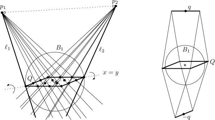
Figure 1: Left: a set $\mathcal{L}$ of nearly vertical lines that intersect a square $Q$ in a grid-like pattern, and their minimum intersecting ball $B_{1}$. Right: a set of four nearly vertical planes containing four sides of a square $Q=[-1,1]^{2}$ in the $xy$-plane, and their minimum intersecting ball $B_{1}$.

Lines in $\mathbb{R}^{3}$.

For an integer $n$ and a polynomial $\lambda(x,y)$, we construct a set $\mathcal{L}$ of $n$ lines in $\mathbb{R}^{3}$. Consider the square $Q=[-1,1]^{2}$ in the $xy$-plane (Fig. 1 (left)). Let $B_{1}$ be the ball of radius $\sqrt{2}$ centered at the origin, and note that $Q\subset B_{1}$. We first construct two skew lines in $\mathbb{R}^{3}$ whose minimum intersecting ball is $B_{1}$. Start with two vertical lines passing through $(1,1,0)$ and $(-1,-1,0)$, and observe that they intersect any horizontal plane at two points at distance $2\sqrt{2}$ apart. Rotate these lines about the horizontal line $\ell_{0}:y=x$ by some small angle $\alpha$ and $-\alpha$, respectively, to obtain two skew lines $\ell_{1}$ and $\ell_{2}$. As $\ell_{1}$ and $\ell_{2}$ remain orthogonal to $\ell_{0}$, the minimum intersecting ball of $\ell_{1}$ and $\ell_{2}$ is still $B_{1}$. Choose $\alpha$ such that $\ell_{1}$ and $\ell_{2}$ intersect the horizontal plane $z=n\,\lambda(n,4)$ at two points, $p_{1}$ and $p_{2}$, at distance $4$ apart. We now define the set $\mathcal{L}$ of $n$ lines as follows: $\mathcal{L}$ contains $\ell_{1}$ and $\ell_{2}$, about half of the lines in $\mathcal{L}$ pass through $p_{1}$ and the other half pass through $p_{2}$. The lines in $\mathcal{L}$ are nearly vertical and intersect $Q$ in a square grid pattern, where any two intersection points are at distance at least $2/\sqrt{n}$ apart.

Lemma 1.

Every TSP tour $\gamma$ lying in $\lambda\,B_{1}$ satisfies ${\rm len}(\gamma)\geq\frac{\sqrt{n}}{8}\,{\rm len}({\rm OPT})$. In particular, $\lambda\,B_{1}$ does not contain the optimal tour ${\rm OPT}={\rm OPT}(\mathcal{L})$ or any $o(\sqrt{n})$-approximation of it.

Proof.

Note that the tour that visits points $p_{1}$ and $p_{2}$, of length $2|p_{1}p_{2}|=8$, intersects all lines. Consequently, ${\rm len}({\rm OPT})\leq 8$ and ${\rm diam}({\rm OPT})\leq 4$. Consider a tour $\gamma$ lying in $\lambda\,B_{1}$ and let $\gamma^{\prime}$ be the orthogonal projection of $\gamma$ onto the $xy$-plane, where ${\rm len}(\gamma^{\prime})\leq{\rm len}(\gamma)$. Since the lines in $\mathcal{L}$ are nearly vertical, the orthogonal projections of the line segments in $\{\ell\cap\lambda\,B_{1}:\ell\in\mathcal{L}\}$ have length at most $2/n$, and they each contain distinct grid points within $Q$. Since the distance between any two grid points is at least $2/\sqrt{n}$, we have ${\rm len}(\gamma^{\prime})\geq n(2/\sqrt{n}-4/n)=2\sqrt{n}-4\geq\sqrt{n}$, and so ${\rm len}(\gamma)\geq\sqrt{n}\geq\frac{\sqrt{n}}{8}\,{\rm len}({\rm OPT})$, as required. ∎

Planes in $\mathbb{R}^{3}$.

For an integer $n$ and a polynomial $\lambda(x,y)$, we construct a set $\mathcal{H}$ of $n$ planes in $\mathbb{R}^{3}$. Consider the unit square $Q=[-1,1]^{2}$ in the $xy$-plane (Fig. 1 (right)). Let the first 4 planes in $\mathcal{H}$ each contain one side of $Q$. The two planes containing the two sides of $Q$ parallel to the $x$-axis intersect in a line parallel to the $x$-axis and containing the point $q=(0,0,h)$, where $h$ is large, specifically $h=n\,\lambda(n,3)$. The two planes containing the sides of $Q$ parallel to the $y$-axis intersect in a line parallel to the $y$-axis and containing the point $-q=(0,0,-h)$. By symmetry, the minimum intersecting ball of these four planes is centered at the origin, and its radius is at least $1-1/h$ and at most $1$. Arrange the remaining $n-4$ planes in $\mathcal{H}$ such that they all contain the point $q=(0,0,h)$, are tangent to the ball $B_{1}$, and the tangency points are uniformly distributed along a horizontal circle $C\subset\partial B_{1}$. By construction, $B_{1}$ is the minimum intersecting ball of the $n$ planes in $\mathcal{H}$.

Lemma 2.

Every TSP tour $\gamma$ lying in $\lambda\,B_{1}$ satisfies ${\rm len}(\gamma)\geq\frac{\pi}{2}(1-O(1/n))\,{\rm len}({\rm OPT})$. In particular, $\lambda\,B_{1}$ does not contain the optimal tour ${\rm OPT}={\rm OPT}(\mathcal{H})$ or any $(1+\varepsilon)$-approximation of it for a sufficiently small $\varepsilon>0$.

Proof.

Note that the triangle formed by the point $q$ and its orthogonal projections onto the two planes containing the two sides of $Q$ parallel to the $y$-axis is a tour for $\mathcal{H}$. The length of this tour is at most $4+4/h$. Consequently, ${\rm len}({\rm OPT})\leq 4+4/h$ and ${\rm diam}({\rm OPT})\leq 3$. Consider a tour $\gamma$ lying in $\lambda\,B_{1}$, and let $\gamma^{\prime}$ be the orthogonal projection of $\gamma$ to the $xy$-plane, where ${\rm len}(\gamma^{\prime})\leq{\rm len}(\gamma)$. Since the planes in $\mathcal{H}$ are nearly vertical, the orthogonal projections of the disks in $\{H\cap\lambda\,B_{1}:H\in\mathcal{H}\}$ are ellipses of width at most $2/n$. The first four ellipses each contain a side of the square $Q$. The remaining ellipses form $\lfloor(n-4)/2\rfloor$ pairs such that the major axes of any pair are on parallel lines at distance at least $2-2/n$ apart, and the directions of the pairs are uniformly distributed. Consequently, the width of $\gamma^{\prime}$ is at least $2-O(1/n)$, and so ${\rm len}(\gamma^{\prime})\geq 2\pi(1-O(1/n))$ $\geq\frac{\pi}{2}(1-O(1/n))\,{\rm len}({\rm OPT})$, as required. ∎

Easy weak approximations.

Finding a minimum-radius ball $B_{1}$ that intersects a set of $n$ hyperplanes (resp., lines) in $\mathbb{R}^{d}$ is an LP-type problem [20]; for a fixed $d$, such a ball can be computed in $O(n)$ time. This immediately leads to a simple $2^{d-1}$-approximation for hyperplanes and a $O(n^{1-1/(d-2)})$-approximation for lines in $\mathbb{R}^{d}$. Indeed, since the minimum enclosing ball $B_{\rm OPT}$ of an optimal tour ${\rm OPT}$ also intersects all $n$ hyperplanes (resp., lines), it is clear that ${\rm diam}(B_{1})\leq{\rm diam}(B_{\rm OPT})$. Since $B_{\rm OPT}$ is spanned by up to $d+1$ points, it is easy to see that ${\rm len}({\rm OPT})\geq 2\,{\rm diam}(B_{\rm OPT})$. On the other hand, a Hamiltonian cycle of the $2^{d}$ vertices of an enclosing hypercube of $B_{1}$ intersects all hyperplanes (cf. Observation 1), and has length at most $2^{d}{\rm diam}(B_{1})$. For $n$ lines in $\mathbb{R}^{d}$, one can compute all intersection points of the $n$ lines with the boundary of $B_{1}$, and return an approximate tour for these $2n$ points of length ${\rm diam}(B_{1})\cdot O(n^{1-1/(d-2)})$ by a result of Few [25].

In Section 3 we obtain a better approximation for TSPN for $n$ hyperplanes, a ratio close to $2^{d-1}/\sqrt{d}$, by using hyperrectangles instead of balls and a careful analysis. In Section 4, we use a completely different approach to achieve a much better $O(\log^{3}n)$-approximation for TSPN for $n$ lines in $\mathbb{R}^{3}$.

3 TSPN for hyperplanes in $\mathbb{R}^{d}$

In this section we prove Theorem 1: we present a constant factor approximation algorithm for TSPN for a set $\mathcal{H}$ of $n$ hyperplanes in $\mathbb{R}^{d}$ with ratio $(1+\varepsilon)\frac{2^{d-1}}{\sqrt{d}}$ and running in $O(n)$ time, for constant $d$ and $\varepsilon>0$. In particular, for $\varepsilon=0.0002$, we get the approximation ratios $2.31$ in $\mathbb{R}^{3}$, $4.001$ in $\mathbb{R}^{4}$, and $7.16$ in $\mathbb{R}^{5}$.

Our algorithm is based on solving low-dimensional linear programs; it combines ideas from [15, 16, 17, 33]. We show below (Lemma 4) that any closed curve $\gamma\subset\mathbb{R}^{d}$ is contained in a rectangular box of edge lengths $w_{1},\ldots,w_{d}$ such that $\sum_{i=1}^{d}w_{i}\leq\frac{\sqrt{d}}{2}\,{\rm len}(\gamma)$. We apply this result to the optimal tour ${\rm OPT}(\mathcal{H})$. Then we use linear programming to compute a $(1+\varepsilon)$-approximation for the minimum-perimeter rectangular box intersecting $\mathcal{H}$, and produce a Hamiltonian cycle of the $2^{d}$ vertices as an approximate tour.

Let $Q$ be rectangular box in $\mathbb{R}^{d}$ such that the $d$ extents of $Q$ are $w_{1}\leq w_{2}\leq\ldots\leq w_{d}$. It is not difficult to see (by induction on $d$) that $Q$ admits a Hamiltonian cycle of total length

$$\tau(Q)=2^{d-1}w_{1}+2^{d-2}w_{2}+\ldots+2w_{d-1}+2w_{d}=w_{d}+\sum_{j=1}^{d}2^{d-j}w_{j}.$$

The orientation of a rectangular box $Q$ in $\mathbb{R}^{d}$ is given by an orthonormal basis whose vectors are parallel to the edges of $Q$. Cover the unit sphere $\mathbb{S}^{d-1}\subset\mathbb{R}^{d}$ with spherical caps of radius $r=\varepsilon/(d-1)$. Since the (spherical) volume of $\mathbb{S}^{d-1}$ is constant, and the volume of a spherical cap of radius $r$ is $\Theta(r^{d-1})=\Theta((d/\varepsilon)^{d-1})$, we can select a set $A=\{\alpha_{1},\ldots,\alpha_{m}\}$ of $m=O(d^{d}\varepsilon^{1-d})$ orientations that cover all possible orientations within an error of $\varepsilon/(d-1)$. That is, for any orientation $\alpha$, there is an orientation $\alpha^{\prime}\in A$ and a matching between the orthogonal bases $\alpha$ and $\alpha^{\prime}$ so that the angle between any two corresponding vectors is at most $\varepsilon/(d-1)$.

Algorithm A1.

• Step 1: Let $m=O(d^{d}\varepsilon^{1-d})$. For each $i=1,\ldots,m$, compute a minimum-perimeter rectangular box $Q_{i}$ with orientation $\alpha_{i}$ that intersects $\mathcal{H}$.

• Step 2: Let $Q$ be a box with the minimum perimeter over all $m$ directions, found above. Return a Hamiltonian cycle of the $2^{d}$ vertices of $Q$, of length $\tau(Q)$, as depicted in Fig. 2 (right).

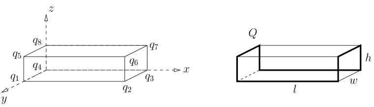
Figure 2: Left: An axis-aligned rectangular box $Q$. Right: a Hamiltonian cycle (in bold lines) of length $2l+2w+4h$ of the vertices of $Q$ that visits all planes intersecting $Q$.

For each iteration $i=1,\ldots,m$, we compute the box $Q_{i}$ by linear programming. By a suitable rotation of the set $\mathcal{H}$ of hyperplanes, the box $Q_{i}$ is axis-aligned. This can be obtained in $O(n)$ time per iteration. For a hyperplane $\sigma$, let $\vec{u}(\sigma)$ denote the unit vector orthogonal to $\sigma$ with a positive $x_{d}$-coordinate. An axis-aligned rectangular box in $\mathbb{R}^{d}$ has $2^{d-1}$ antipodal pairs of vertices, which we denote by $s_{j}$ and $t_{j}$, for $j=1,\ldots,2^{d-1}$, such that the vector $s_{j}t_{j}$ has a positive $x_{d}$-coordinate. Partition $\mathcal{H}$ into $2^{d-1}$ types based on the following rule (ties are broken arbitrarily):

• $\sigma\in\mathcal{H}$ is of type $j$, $j\in\{1,\ldots,2^{d-1}\}$, if the $\vec{u}(\sigma)$-minimal and $\vec{u}(\sigma)$-maximal vertices of $Q_{i}$ are $s_{j}$ and $t_{j}$, respectively.

Let $\mathcal{H}=\bigcup_{j=1}^{2^{d-1}}\mathcal{H}_{i}$ be the corresponding partition of the hyperplanes given by this rule. For a hyperplane $\sigma$, that is not parallel to any coordinate axis, denote by $\sigma(p)\leq 0$ (respectively, by $\sigma(p)\geq 0$) that a point $p\in\mathbb{R}^{d}$ lies in the closed halfspace bounded from above by $\sigma$ (resp., bounded from below by $\sigma$). Observe that for $j=1,\ldots 2^{d-1}$,

• a hyperplane $\sigma\in\mathcal{H}_{j}$ intersects the rectangular box $Q_{i}$ if and only if $\sigma(s_{j})\leq 0\leq\sigma(t_{j})$.

The minimum-perimeter objective is naturally expressed as a linear function. The resulting linear program has $2d$ variables $x_{1},y_{1},\ldots,x_{d},y_{d}$ for the box $Q_{i}=[x_{1},y_{1}]\times\ldots\times[x_{d},y_{d}]$, and $2n+d$ constraints.

minimize $$\sum_{k=1}^{d}(y_{k}-x_{k})\ \ \ \quad\quad\textup{(LP1)}$$

subject to $$\left\{\begin{array}[]{lll}\sigma(s_{j})\leq 0&\mbox{ \rm if }\sigma\in\mathcal{H}_{j},&\forall\sigma\in\mathcal{H}\\ \sigma(t_{j})\geq 0&\mbox{ \rm if }\sigma\in\mathcal{H}_{j},&\forall\sigma\in\mathcal{H}\\ x_{k}\leq y_{k}&&\forall k\in\{1,\ldots,d\}\end{array}\right.$$

Algorithm analysis.

The key observation is the following.

Observation 1.

• If a polygon $\gamma$ intersects $\mathcal{H}$, then ${\rm conv}(\gamma)$, and any other set containing ${\rm conv}(\gamma)$, also intersects $\mathcal{H}$.

• If a convex polytope $Q$ intersects $\mathcal{H}$, then every Hamiltonian cycle of the vertices of $Q$ also intersects $\mathcal{H}$.

Let $Q^{*}$ be a minimum-perimeter rectangular box intersecting $\mathcal{H}$, with side lengths denoted by $w_{1},\ldots,w_{d}$. To account for the error made by discretization, we need the following easy fact. The planar variant was shown in [16, Lemma 2]. We include the almost identical proof for completeness.

Lemma 3.

There exists $i\in\{1,\ldots,m\}$ such that ${\rm per}(Q_{i})\leq(1+\varepsilon)\,{\rm per}(Q^{*})$.

Proof.

Consider a box $Q_{i}$, $i\in\{1,\ldots,m\}$, that minimizes the angle difference $\beta$ between the orientations of $Q_{i}$ and $Q^{*}$. By construction, there exists $i\in\{1,\ldots,m\}$ such that the angle $\beta$ between the orientations of $Q_{i}$ and $Q^{*}$ is at most $\varepsilon/(d-1)$, that is, $\beta\leq\varepsilon/(d-1)$.

Let $Q_{i}^{\prime}$ be the minimum-perimeter box with the same orientation as $Q_{i}$ such that $Q_{i}^{\prime}$ contains $Q^{*}$. By definition, ${\rm per}(Q_{i})\leq{\rm per}(Q^{\prime}_{i})$. An easy trigonometric calculation shows that the corresponding sides $w_{1}^{\prime},\ldots,w_{d}^{\prime}$ of $Q_{i}^{\prime}$ are bounded from above as follows. For $j=1,\ldots,d$, we have

$$w_{j}^{\prime}\leq w_{j}\cos\beta+\left(\sum_{k\neq j}w_{k}\right)\sin\beta\leq w_{j}+\left(\sum_{k\neq j}w_{k}\right)\,\frac{\varepsilon}{d-1}.$$

Consequently,

$$\sum_{j=1}^{d}w_{j}^{\prime}\leq(1+\varepsilon)\sum_{j=1}^{d}w_{j},$$

that is,

$${\rm per}(Q^{\prime}_{i})\leq(1+\varepsilon)\,{\rm per}(Q^{*}).$$

Since ${\rm per}(Q_{i})\leq{\rm per}(Q^{\prime}_{i})$, it follows that ${\rm per}(Q_{i})\leq(1+\varepsilon)\,{\rm per}(Q^{*})$, as required. ∎

Lemma 4.

A closed curve $\gamma\subset\mathbb{R}^{d}$ is contained in a rectangular box $Q$ with side lengths $w_{1},\ldots,w_{d}$ satisfying $\sum_{j=1}^{d}w_{j}\leq\frac{\sqrt{d}}{2}\,{\rm len}(\gamma)$. Consequently, ${\rm per}(Q)\leq\sqrt{d}\cdot 2^{d-2}\,{\rm len}(\gamma)$.

Proof.

Let $\gamma$ be a closed curve and let $Q=Q(\gamma)$ be a minimum-perimeter enclosing rectangular box. Assume for convenience that $Q$ is axis-aligned, so that its extents in the $d$ coordinates are $w_{1},\ldots,w_{d}$, respectively. Since $Q$ has minimum perimeter, $\gamma$ meets each $(d-1)$-dimensional face of $Q$. Arbitrarily select a point $a_{i}$ of $\gamma$ on each of the $2d$ faces of $Q$, in the order traversed by $\gamma$, to obtain a polygonal closed curve $\gamma_{1}=(a_{1},\ldots,a_{2d})$ still enclosed in $Q$ (duplicate points are possible). For convenience, introduce $a_{2d+1}=a_{1}$.

By the triangle inequality,

$${\rm len}(\gamma)\geq{\rm len}(\gamma_{1})=\sum_{i=1}^{2d}{\rm len}(a_{i}a_{i+1}).$$ (1)

By the Cauchy-Schwarz inequality, for $i=1,\ldots,2d$, we have

$${\rm len}(a_{i}a_{i+1})=\left(\sum_{j=1}^{d}\Delta_{j}^{2}(a_{i}a_{i+1})\right)^{1/2}\geq\frac{1}{\sqrt{d}}\sum_{j=1}^{d}\Delta_{j}(a_{i}a_{i+1}).$$ (2)

Since $\gamma_{1}$ is a closed curve that visits both faces of $Q$ orthogonal to the $j$th axis for each $j=1,\ldots,d$, we have

$$\sum_{i=1}^{2d}\Delta_{j}(a_{i}a_{i+1})\geq 2w_{j},\text{ for }j=1,\ldots,d.$$

Combined with (1) and (2), this yields ${\rm len}(\gamma)\geq\frac{2}{\sqrt{d}}\sum_{j=1}^{d}w_{j}$, as claimed. ∎

Let $L^{*}={\rm len}({\rm OPT})$ and let $Q_{\rm OPT}$ be a minimum-perimeter rectangular box containing ${\rm OPT}$. By Observation 1 and Lemmas 3 and 4, we have

$${\rm per}(Q_{i})\leq(1+\varepsilon){\rm per}(Q^{*})\leq(1+\varepsilon){\rm per}(Q_{\rm OPT})\leq(1+\varepsilon)\sqrt{d}\cdot 2^{d-2}L^{*}.$$ (3)

By Observation 1, any Hamiltonian cycle of $Q_{i}$ is a valid tour of the hyperplanes in $\mathcal{H}$, and its length is bounded above by ${\rm per}(Q_{i})$. From (3), this length is at most $(1+\varepsilon)\sqrt{d}\cdot 2^{d-2}$ times the optimum.

We now refine the analysis and show that the length $\tau(Q_{i})$ of a shortest Hamiltonian cycle of $Q_{i}$ is at most $2^{d-1}/\sqrt{d}$ times the optimum. Algorithm A1 computes a tour $T$ of length $L=\tau(Q_{i})=w_{d}+\sum_{j=1}^{d}2^{d-j}w_{j}$, where $\sum_{j=1}^{d}w_{j}\leq(1+\varepsilon)\frac{\sqrt{d}}{2}L^{*}$. For $i=1,\ldots,d$ put $S_{i}=\sum_{j=1}^{i}w_{j}$ and $S=S_{d}$. Since $w_{1}\leq w_{2}\ldots\leq w_{d}$, we have $S_{i}\leq iS/d$, for $i=1,\ldots,d$. Consequently,

$$L =w_{d}+\sum_{j=1}^{d}2^{d-j}w_{j}=2^{d-1}w_{1}+2^{d-2}w_{2}+\ldots+2w_{d-1}+2w_{d}$$

$$=2S_{d}+\sum_{i=1}^{d-2}2^{i}S_{d-i-1}\leq\frac{S}{d}\left(2d+\sum_{i=1}^{d-2}2^{i}(d-i-1)\right)$$

$$=\frac{S}{d}\left(\left(2d+d\sum_{i=1}^{d-2}2^{i}\right)-\sum_{i=1}^{d-2}(i+1)2^{i}\right)$$

$$=\frac{S}{d}\left(d\,2^{d-1}-(d-2)\,2^{d-1}\right)=\frac{2^{d}}{d}\,S.$$ (4)

To evaluate $\sum_{i=1}^{d-2}(i+1)2^{i}$ in the last line of (3), we set $F(x)=\sum_{i=2}^{d-1}x^{i}$, and evaluate its derivative $F^{\prime}(x)$ in two ways (we omit the details). Substituting now the upper bound $S\leq(1+\varepsilon)\frac{\sqrt{d}}{2}L^{*}$ yields

$$L\leq\frac{2^{d}}{d}\,S\leq(1+\varepsilon)\frac{\sqrt{d}}{2}\,\frac{2^{d}}{d}L^{*}=(1+\varepsilon)\frac{2^{d-1}}{\sqrt{d}}L^{*},$$

as required.

A rough upper estimate on the running time accounts for $m=O(d^{d}\varepsilon^{1-d})$ $2d$-dimensional linear programs, each solved in $O(d^{2}2^{2d}\,n)$ time [10, 36]. The overall running time is $O(C_{d,\varepsilon}\ n)$, where $C_{d,\varepsilon}=d^{2}2^{2d}\,(d/\varepsilon)^{d}$.

In particular, for $d=3$ and $\varepsilon\leq 0.00022$, we have $L\leq 2.31L^{*}$, thus algorithm A1 computes a tour whose length is at most $2.31$ times the optimal. The algorithm solves a (large!) constant number of $6$-dimensional linear programs, each in $O(n)$ time [38]. The overall time is $O(n)$. A modest number of linear programs suffices to get a weaker approximation, say $2.5$ or $3$.

Remark.

A standard reduction from the sorting problem or from the convex hull problem as in [45], applied to a suitable set of hyperplanes, shows that a shortest TSP tour for $n$ hyperplanes in $\mathbb{R}^{d}$, $d\geq 2$, cannot be computed in $O(n)$ time; that is, in the worst-case, finding an optimal tour requires $\Omega(n\log{n})$ time in the algebraic decision tree model of computation.

4 TSPN for lines in $\mathbb{R}^{d}$

In this section we prove Theorem 2. Let $\mathcal{L}=\{\ell_{1},\ldots,\ell_{n}\}$ be a set of $n$ lines in $\mathbb{R}^{d}$, $d\geq 3$. If all lines are parallel, we reduce TSPN for $\mathcal{L}$ to TSP for the $n$ intersection points of the lines with an arbitrary orthogonal hyperplane. Otherwise, we reduce the TSPN problem to a group Steiner tree problem on a geometric graph. Specifically, we construct a geometric graph $G_{\mathcal{L}}=(V,E)$, where $V$ is a set of points on the lines in $\mathcal{L}$, and $E$ consists of line segments connecting some of these points; the weight of an edge is its Euclidean length. We have $V=\bigcup_{i=1}^{n}V_{i}$, where $V_{i}\subset\ell_{i}$ ($i=1,\ldots,n$) naturally form $n$ groups, one for each line. We then run an approximation algorithm for the group Steiner tree problem on this graph.

It is well known that an optimal TSP tour for points can be 2-approximated by a minimum spanning tree (a TSP tour is obtained by doubling the edges of the MST and by using shortcuts and the triangle inequality). Reich and Widmayer [47] introduced the following group Steiner tree (a.k.a., one-of-a-set Steiner tree) problem. Given an edge weighted graph $G=(V,E)$ and $g$ groups of vertices $V_{1},\ldots,V_{g}\subseteq V$, $|V|=n$, find a tree of minimum weight in $G$ that includes at least one vertex from each group. The problem is known to be APX-hard [5], and it cannot be approximated better than $\Omega(\log^{2-\varepsilon}n)$ for any $\varepsilon>0$ unless NP admits quasipolynomial-time Las Vegas algorithms [31]. The current best approximation ratio, $O(\log^{2}n\log g)$ comes from the algorithm of Garg et al. [29] as further refined by Fakcharoenphol et al. [24]. As before with the MST, by doubling the edges of such a tree, and by using shortcuts and the triangle inequality, one can obtain a Hamiltonian cycle which includes at least one vertex from each group, and the approximation ratio of this cycle is of the same asymptotic order as the approximation ratio of the group Steiner tree used.

The key Lemma 7 below shows that the length of a minimum group Steiner tree in $G_{\mathcal{L}}$ (the graph used by the algorithm) is a constant-factor approximation for the minimum TSP tour for $\mathcal{L}$. In our case, the graph $G_{\mathcal{L}}$ has $O(n^{3})$ vertices and the number of groups is $n$, so the $O(\log^{2}n\log g)$-approximation [24, 29] for the group Steiner tree problem on a graph with $n$ vertices and $g$ groups yields an $O(\log^{3}n)$-approximation for TSPN for $n$ lines in $\mathbb{R}^{d}$.

Construction of graph $G_{\mathcal{L}}$.

A transversal between two lines, $\ell_{i}$ and $\ell_{j}$, is a line segment $t_{i,j}t_{j,i}$ with $t_{i,j}\in\ell_{i}$ and $t_{j,i}\in\ell_{j}$. A minimum transversal of two lines is one of minimum length; it is orthogonal to both lines, and if the two lines intersect, it is a segment of zero length (i.e., $t_{i,j}=t_{j,i}$). A pair of skew lines admits a unique minimal transversal.

We define $G_{\mathcal{L}}$ in terms of a set $S$ of transversal segments among the lines: let the vertices of $G_{\mathcal{L}}$ be the set of endpoints of the segments in $S$; the edges of $G_{\mathcal{L}}$ include all segments in $S$, and all segments along the lines in $\mathcal{L}$ between consecutive vertices. We use two types of transversal segments, $S_{1}$ and $S_{2}$, with $S=S_{1}\cup S_{2}$. Let $S_{1}$ be the set of minimum transversals between all pairs of nonparallel lines in $\mathcal{L}$. To define $S_{2}$, we proceed as follows; see Fig. 3 (left). For each ordered pair of nonparallel lines $(\ell_{i},\ell_{j})\in\mathcal{L}^{2}$, let $T_{i,j}$ be the hyperplane orthogonal to $\ell_{i}$ and containing $t_{i,j}$, and let $P_{i,j}=\{T_{i,j}\cap\ell:\ell\in\mathcal{L}\}$ be the set of intersection points of $T_{i,j}$ with the lines in $\mathcal{L}$. Note that $t_{i,j}\in P_{i,j}$ and $|P_{i,j}|\leq n$. Add all edges of the complete graph on $P_{i,j}$ to the set $S_{2}$.

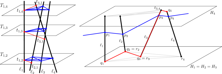
Figure 3: Left: A set of four lines $\ell_{1},\ldots,\ell_{4}$. The minimum transversals between $\ell_{1}$ and the other three lines are $t_{1,2}t_{2,1}$, $t_{1,3}t_{3,1}$ and $t_{1,4}t_{4,1}$. For $i=1,2,3$, we insert a complete graph in the plane $T_{1,i}$ orthogonal to $\ell_{1}$ and incident to $t_{1,i}$. Right: An optimal tour ${\rm OPT}$ visits the lines $\ell_{1},\ell_{2},\ell_{3},\ell_{4}$ at points $p_{1},p_{2},p_{3},p_{4}$, respectively. We construct a path $\gamma_{1}=(q_{1}q_{2}q_{3}q_{4})$ that visits these lines in the same order. Points $q_{1},q_{2},q_{3}$ are in the same hyperplane $H_{1}=H_{2}=H_{3}$. Point $q_{4}$ is in a hyperplane $H_{4}\neq H_{3}$ because $|q_{3}r_{4}|>3|p_{3}p_{4}|$.

The set of transversals $S=S_{1}\cup S_{2}$ determines $G_{\mathcal{L}}$. The segments in $S_{1}$ have at most $n(n-1)$ endpoints, and for each segment endpoint we compute a complete graph, each with at most $n$ vertices and ${n\choose 2}$ edges, thus $S_{2}$ contains $O(n^{4})$ segments and $|S|=|S_{1}\cup S_{2}|=O(n^{2}+n^{4})=O(n^{4})$. Consequently, $G_{\mathcal{L}}$ has $O(n^{3})$ vertices and $|S|+O(n^{3})=O(n^{4})$ edges. The vertices in $G_{\mathcal{L}}$ are partitioned into $n$ groups, one for each line $\ell\in\mathcal{L}$. The group corresponding to line $\ell$ contains all $O(n^{2})$ endpoints of transversal segments in $S$ on $\ell$.

The minimum transversal of two skew lines in $\mathbb{R}^{d}$ lies in the 3-dimensional affine subspace spanned by the lines, and it can be computed in $O(d)$ time; point-hyperplane intersections can also be computed in $O(d)$ time in $\mathbb{R}^{d}$. Consequently, the graph $G_{\mathcal{L}}$ can we computed in $O(dn^{4})$ time.

Two technical lemmas.

The approximation relies on Lemmas 5 and 6 (below). According to Lemma 5, if the directions of two lines are far apart, then a connecting segment can be approximated by a $3$-segment path that detours through the minimum transversal of the two lines. According to Lemma 6, if two lines are nearly vertical and we are given some horizontal transversal segment between the lines, then the only way to find a significantly shorter transversal is to move the endpoints closer to the endpoints of the minimum transversal.

Figure 4: Left: The angle between lines $\ell_{1}$ and $\ell_{2}$ is $\varphi$. The distance between $p_{1}\in\ell_{1}$ and $p_{2}\in\ell_{2}$ is approximated by the polygonal path $(p_{1},s_{1},s_{2},p_{2})$ that passes through the minimum transversal $s_{1}s_{2}$ between the two lines. Middle: If $|p_{1}p_{2}|\leq\frac{1}{3}|r_{1}r_{2}|$, then $p_{1}$ and $p_{2}$ are much closer to the minimum transversal than $r_{1}$ and $r_{2}$, respectively. Right: Two triangles with angle $\varphi$. The other two angles are equal in one triangle, and they differ by at most $2\psi$ in the other triangle.

Lemma 5.

Let $\ell_{1}$ and $\ell_{2}$ be two lines in $\mathbb{R}^{d}$ such that the angle between their directions is $\varphi\in(\varphi_{0},\frac{\pi}{2}]$. Let $t_{1,2}t_{2,1}$ be their minimum transversal with $t_{1,2}\in\ell_{1}$ and $t_{2,1}\in\ell_{2}$. Let $p_{1}\in\ell_{1}$ and $p_{2}\in\ell_{2}$ be two points. Then $|p_{1}t_{1,2}|+|t_{1,2}t_{2,1}|+|t_{2,1}p_{2}|\leq\sqrt{\frac{3}{1-\cos\varphi_{0}}}|p_{1}p_{2}|.$

Proof.

Consider the 3-dimensional affine subspace spanned by $\ell_{1}$ and $\ell_{2}$. Without loss of generality, we may assume that $\ell_{1}$ is the $x$-axis, $p_{1}=(a,0,0)$, $t_{1,2}=(0,0,0)$, and $t_{2,1}=(0,0,h)$ as in Fig. 4 (left). Let $a=|p_{1}t_{1,2}|$ and $b=|p_{2}t_{2,1}|$. The Cauchy-Schwarz inequality yields the upper bound

$$|p_{1}t_{1,2}|+|t_{1,2}t_{2,1}|+|t_{2,1}p_{1}|=a+h+b\leq\sqrt{3(a^{2}+b^{2}+h^{2})}.$$

If $x(p_{2})\geq 0$ (as in Fig. 4, left), then the law of cosines yields

$$|p_{1}p_{2}|^{2} = h^{2}+a^{2}+b^{2}-2ab\cos\varphi$$

$$= h^{2}+(a-b)^{2}\cos\varphi+(a^{2}+b^{2})(1-\cos\varphi)$$

$$\geq (1-\cos\varphi)(a^{2}+b^{2}+h^{2})$$

$$\geq (1-\cos\varphi_{0})(a^{2}+b^{2}+h^{2}).$$

If $x(p_{2})\leq 0$, then $|p_{1}p_{2}|^{2}=h^{2}+a^{2}+b^{2}-2ab\cos(\pi-\varphi)\geq h^{2}+a^{2}+b^{2}$, since $\cos(\pi-\varphi)<0$, and we obtain $|p_{1}p_{2}|^{2}\geq(1-\cos\varphi_{0})(a^{2}+b^{2}+h^{2})$ in this case, as well. In both cases, the claimed inequality follows after taking square roots. ∎

Lemma 6.

Let $\ell_{1}$ and $\ell_{2}$ be two lines in $\mathbb{R}^{d}$ such that the angle between their directions is $\varphi\in(0,\frac{\pi}{6}]$; and the direction of each line differs from the $x_{d}$-axis by at most $\psi\in[0,\frac{\pi}{6}]$. Let $p_{1}\in\ell_{1}$ and $p_{2}\in\ell_{2}$ be two arbitrary points on the two lines; let $r_{1}\in\ell_{1}$ and $r_{2}\in\ell_{2}$ be the intersection points of the two lines with a hyperplane orthogonal to the $x_{d}$-axis; and $t_{1,2}t_{2,1}$ be the minimum transversal of the two lines such that $t_{1,2}\in\ell_{1}$ and $t_{2,1}\in\ell_{2}$ (Fig. 4, middle). If $3|p_{1}p_{2}|\leq|r_{1}r_{2}|$, then $|p_{1}t_{1,2}|\leq\frac{2\sqrt{3}}{9}\ |r_{1}t_{1,2}|$ and $|p_{2}t_{2,1}|\leq\frac{2\sqrt{3}}{9}\ |r_{2}t_{2,1}|$.

Proof.

Let $h=|t_{1,2}t_{2,1}|$ be the distance between the two lines. Put $a=|p_{1}t_{1,2}|$, $b=|p_{2}t_{2,1}|$, $e=|r_{1}t_{1,2}|$, and $f=|r_{2}t_{2,1}|$. Let $\varphi_{p}\in\{\varphi,\pi-\varphi\}$ be the angle between the rays $\overrightarrow{t_{1,2}p_{1}}$ and $\overrightarrow{t_{2,1}p_{2}}$. By the law of cosines, we have $|p_{1}p_{2}|^{2}=h^{2}+a^{2}+b^{2}-2ab\cos\varphi_{p}$. The sum of the last three terms in this expression is $c^{2}=a^{2}+b^{2}-2ab\cos\varphi_{p}$, where $c$ is the third side of a triangle with two adjacent sides of lengths $a$ and $b$ that meet at angle $\varphi_{p}$. Denote by $\beta$ the angle of this triangle opposite to the longer of $a$ and $b$. Then the law of sines yields

$$a^{2}+b^{2}-2ab\cos\varphi_{p}=(\max\{a,b\})^{2}\cdot\frac{\sin^{2}\varphi_{p}}{\sin^{2}\beta}\geq(\max\{a,b\})^{2}\sin^{2}\varphi_{p}=(\max\{a,b\})^{2}\sin^{2}\varphi.$$

Consequently,

$$|p_{1}p_{2}|^{2}\geq h^{2}+(\max\{a,b\})^{2}\sin^{2}\varphi.$$ (5)

Let $\varphi_{r}\in\{\varphi,\pi-\varphi\}$ be the angle between the rays $\overrightarrow{t_{1,2}r_{1}}$ and $\overrightarrow{t_{2,1}r_{2}}$. We show that $\varphi_{r}=\varphi$. Indeed, since $r_{1}r_{2}$ lies in a hyperplane orthogonal to the $x_{d}$-axis, and the direction of each line differs from the $x_{d}$-axis by at most $\psi\in[0,\frac{\pi}{6}]$, the directions of $r_{1}r_{2}$ and the minimal transversal $t_{1,2}t_{2,1}$ differ by at most $\frac{\pi}{6}$. If $\varphi_{r}=\pi-\varphi\geq\frac{5\pi}{6}$, then $|r_{1}t_{1,2}|\leq h\tan\frac{\pi}{6}$ and $|r_{2}t_{2,1}|\leq h\tan\frac{\pi}{6}$. The triangle inequality yields $|r_{1}r_{2}|\leq|r_{1}t_{1,2}|+|t_{1,2}t_{2,1}|+|t_{2,1}r_{2}|\leq(1+2\tan\frac{\pi}{6})h=(1+\frac{2\sqrt{3}}{3})h\leq 2.16h$, in contradiction with the assumed inequality $|r_{1}r_{2}|\geq 3|p_{1}p_{2}|\geq 3h$.

By the law of cosines we have

$$|r_{1}r_{2}|^{2}=h^{2}+e^{2}+f^{2}-2ef\cos\varphi_{r}=h^{2}+e^{2}+f^{2}-2ef\cos\varphi.$$

Consider a triangle where $e$ and $f$ are adjacent sides parallel with $r_{1}t_{1,2}$ and $r_{2}t_{2,1}$ respectively, that meet at angle $\varphi$. Since the directions of $\ell_{1}$ and $\ell_{2}$ differ from vertical by at most $\psi$, the angle opposite to the shorter of $e$ and $f$ is at least $\frac{\pi}{2}-\psi$ (see Fig. 4, right). Hence the law of sines yields $e^{2}+f^{2}-2ef\cos\varphi\leq(\min\{e,f\})^{2}\cdot\frac{\sin^{2}\varphi}{\sin^{2}(\pi/2-\psi)}$, and consequently

$$|r_{1}r_{2}|^{2}\leq h^{2}+(\min\{e,f\})^{2}\cdot\frac{\sin^{2}\varphi}{\sin^{2}(\pi/2-\psi)}.$$ (6)

The inequality $3|p_{1}p_{2}|\leq|r_{1}r_{2}|$ in combination with inequalities (5) and (6) implies

$$9\left(h^{2}+\left(\max\{a,b\}\right)^{2}\sin^{2}\varphi\right) \leq h^{2}+\left(\min\{e,f\}\right)^{2}\frac{\sin^{2}\varphi}{\sin^{2}(\pi/2-\psi)},$$

$$9\left(\max\{a,b\}\right)^{2}\sin^{2}\varphi \leq \left(\min\{e,f\}\right)^{2}\frac{\sin^{2}\varphi}{\sin^{2}(\pi/2-\psi)},$$ (7)

and further (after canceling $\sin^{2}\varphi$ and taking square roots) that

$$\max\{a,b\}\leq\frac{\min\{e,f\}}{3\sin(\pi/2-\psi)}.$$ (8)

If $\psi\in[0,\frac{\pi}{6}]$, then $\sin\left(\frac{\pi}{2}-\psi\right)\geq\sin\left(\frac{\pi}{3}\right)=\frac{\sqrt{3}}{2}$ and so $\max\{a,b\}\leq\frac{2\sqrt{3}}{9}\min\{e,f\}$. It follows that $a\leq\frac{2\sqrt{3}}{9}e$ and $b\leq\frac{2\sqrt{3}}{9}f$, as required. ∎

Group Steiner tree yields a constant-factor approximation for TSP with lines.

The main result of this section is the following lemma. Theorem 2 then directly follows from this lemma.

Lemma 7.

Let $\mathcal{L}$ be a set of $n$ lines in $\mathbb{R}^{d}$. Then the length of a minimum group Steiner tree in $G_{\mathcal{L}}$ is $O(1)$ times the length of a minimum TSP tour for the lines in $\mathcal{L}$.

Proof.

Let $\mathcal{L}=\{\ell_{1},\ldots,\ell_{n}\}$, where the lines are indexed so that an optimal TSP tour is ${\rm OPT}(\mathcal{L})=(p_{1},\ldots,p_{n})$ with $p_{i}\in\ell_{i}$, $i=1,\ldots,n$. We show that $G_{\mathcal{L}}$ contains a group Steiner tree $T$ of length at most $83\,{\rm len}({\rm OPT}(\mathcal{L}))$. The argument does not use the optimality of the tour ${\rm OPT}(\mathcal{L})$, i.e., for any cycle $C=(p_{1},\ldots,p_{n})$, $p_{i}\in\ell_{i}$, we construct a group Steiner tree $T$ of length at most $83\,{\rm len}(C)$. The tree $T$ consists of a main (backbone) path $\gamma_{0}$, and a path attached to each vertex of the backbone.

Decompose the cyclic sequence $(\ell_{1},\ldots,\ell_{n})$ into maximal subsequences, called blocks,

$$(\ell_{\tau(i)},\ell_{\tau(i)+1},\ldots,\ell_{\tau(i+1)-1}),\hskip 36.135pti=1,2,\ldots,k$$

for some $k\geq 1$ as follows. Let $\tau(1)=1$, and for each $i=1,\ldots,k-1$, let $\tau(i+1)$ be the first index such that the directions of $\ell_{\tau(i)}$ and $\ell_{\tau(i+1)}$ differ by more than $\frac{\pi}{12}$. That is, the directions of the lines in the $i$-th block differ from the direction of $\ell_{\tau(i)}$ by at most $\frac{\pi}{12}$. By the triangle inequality, the directions of any two lines in a block differ by at most $\frac{\pi}{6}$ (as required by Lemma 6).

Consider the sequence of the first elements of the blocks, $(\ell_{\tau(1)},\ell_{\tau(2)},\ldots,\ell_{\tau(k)})$. By construction, the directions of any two consecutive lines in the above sequence differ by more than $\frac{\pi}{12}$. If $k\geq 2$, the “backbone” of the group Steiner tree $T$ is the polygonal path

$$\gamma_{0}=(t_{\tau(1),\tau(2)}\,t_{\tau(2),\tau(1)}\,t_{\tau(2),\tau(3)}\,t_{\tau(3),\tau(2)}\ldots t_{\tau(k-1),\tau(k)}\,t_{\tau(k),\tau(k-1)}).$$

Lemma 5 with $\varphi_{0}=\frac{\pi}{12}$ implies that ${\rm len}(\gamma_{0})$ is bounded from above as follows:

$${\rm len}(\gamma_{0}) = {\rm len}(t_{\tau(1),\tau(2)}\,t_{\tau(2),\tau(1)}\,t_{\tau(2),\tau(3)}\,t_{\tau(3),\tau(2)}\ldots t_{\tau(k-1),\tau(k)}\,t_{\tau(k),\tau(k-1)})$$ (9)

$$\leq {\rm len}(p_{\tau(1)}\,t_{\tau(1),\tau(2)}\,t_{\tau(2),\tau(1)}\,p_{\tau(2)})+\ldots+{\rm len}(p_{\tau(k-1)}\,t_{\tau(k-1),\tau(k)}\,t_{\tau(k),\tau(k-1)}\,p_{\tau(k)})$$

$$\leq \sqrt{\frac{3}{1-\cos(\pi/12)}}\ {\rm len}(p_{\tau(1)}p_{\tau(2)}\ldots p_{\tau(k)})$$

$$\leq 9.4\ {\rm len}(p_{1}p_{2}\ldots p_{n})\leq 9.4\ {\rm len}(C).$$

For each block $(\ell_{\tau(i)},\ell_{\tau(i)+1},\ldots,\ell_{\tau(i+1)-1})$, $i=1,\ldots,k$, we attach a path $\gamma_{i}$ visiting the lines in this block to the backbone $\gamma_{0}$. Each path $\gamma_{i}$ is constructed incrementally starting from an initial vertex and an initial hyperplane containing that vertex. If $k\geq 2$, then $\gamma_{i}$ starts from vertex $t_{\tau(i),\tau(i+1)}\in\ell_{\tau(i)}\cap\gamma_{0}$ within hyperplane $T_{\tau(i),\tau(i+1)}$ for $i=1,\ldots,k-1$; and $\gamma_{k}$ starts from vertex $t_{\tau(k),\tau(k-1)}\in\ell_{\tau(k)}\cap\gamma_{0}$ within hyperplane $T_{\tau(k),\tau(k-1)}$. If $k=1$ (i.e., there is only one block), then $\gamma_{0}$ is not needed, and we set $T:=\gamma_{1}$. In this case, we construct a path $\gamma_{1}$ starting from each of the $O(n^{2})$ vertices on $\ell_{1}$ and every possible hyperplane of the form $T_{i,j}$ containing that vertex; and then show that one of these paths satisfies ${\rm len}(\gamma_{1})\leq 9.77\,{\rm len}(C)$.

The paths $\gamma_{i}$, $i=1,\ldots,k$, are constructed analogously apart from the choice of their initial vertex $q_{1}$ and initial hyperplane $H_{1}$, $q_{1}\in H_{1}$. We explain the construction for $i=1$ only. Consider the first block, $(\ell_{1},\ell_{2},\ldots,\ell_{m})$, where $1\leq m\leq n$. The path $\gamma_{1}$ will use transversal segments from $S_{2}$ between lines in $\ell_{1},\ldots,\ell_{m}$, and possibly some edges along the lines $\ell_{1},\ldots,\ell_{m}$.

We construct $\gamma_{1}$ incrementally for a given initial vertex $q_{1}$ and hyperplane $H_{1}$, $q_{1}\in H_{1}$. Refer to Fig. 3 (right). In each step, we maintain a vertex $q_{i}\in\ell_{i}$ of $\gamma_{1}$ and hyperplane $H_{i}$ such that $q_{i}\in H_{i}$ and $G_{\mathcal{L}}$ contains a complete graph on the intersection points between the lines in $\mathcal{L}$ and $H_{i}$. Initially, we have a single-vertex path $\gamma_{1}=(q_{1})$, where $q_{1}\in\ell_{1}$ and $q_{1}\in H_{1}$. We extend $\gamma_{1}$ in $m-1$ steps to visit some points $q_{i}\in\ell_{i}$, $i=2,\ldots,m$. In step $i$, we would like to extend $\gamma_{1}$ from $q_{i}$ to $q_{i+1}\in\ell_{i+1}$ by a single edge in $H_{i}$. However, if the distance from $q_{i}$ to $\ell_{i+1}\cap H_{i}$ is more than $3\ |p_{i}p_{i+1}|$, then $\gamma_{1}$ will follow $\ell_{i}$ to the endpoint $t_{i,i+1}$ of the minimal transversal between $\ell_{i}$ and $\ell_{i+1}$, and reach $\ell_{i+1}$ in the hyperplane $T_{i,i+1}$ (orthogonal to $\ell_{i}$).

Assume that we have already built the path $\gamma_{1}$ up to vertex $q_{i}\in\ell_{i}$, $i\in\{1,\ldots,m-1\}$, with a hyperplane $H_{i}$, $q_{i}\in H_{i}$. We choose $q_{i+1}\in\ell_{i+1}$, the portion of $\gamma_{1}$ from $q_{i}$ to $q_{i+1}$, and the hyperplane $H_{i+1}$ as follows. Let $r_{i+1}=\ell_{i+1}\cap H_{i}$ (note that $r_{i+1}$ is a vertex of $G_{\mathcal{L}}$ by construction). We distinguish two cases:

• If $|q_{i}r_{i+1}|\leq 3\ |p_{i}p_{i+1}|$, then let $q_{i+1}=r_{i+1}$, extend the path $\gamma_{1}$ with the edge $q_{i}q_{i+1}\subset H_{i}$, and let $H_{i+1}=H_{i}$.

• Otherwise let $H_{i+1}=T_{i,i+1}$ (the hyperplane orthogonal to $\ell_{i}$ and containing $t_{i,i+1}$), and let $q_{i+1}=\ell_{i+1}\cap H_{i+1}$. Now extend $\gamma_{1}$ with the segments $q_{i}t_{i,i+1}\subset\ell_{i}$ and $t_{i,i+1}q_{i+1}\subset H_{i+1}$.

For estimating ${\rm len}(\gamma_{1})$, we consider the transversal segments and the edges along the lines in $\mathcal{L}$ separately. The length of the transversal segment between $\ell_{i}$ and $\ell_{i+1}$ is at most $3\,|p_{i}p_{i+1}|$, and consequently, the total length of all transversal segments in $\gamma_{1}$ is at most $3\,{\rm len}(p_{1}\ldots p_{m})$. Indeed, in the first case $H_{i}$ contains the edge $q_{i}q_{i+1}$ of length $|q_{i}q_{i+1}|=|q_{i}r_{i+1}|\leq 3\ |p_{i}p_{i+1}|$. In the second case, $H_{i+1}$ contains segment $t_{i,i+1}\,q_{i+1}$ of length

$$|t_{i,i+1}\,q_{i+1}|\leq\frac{1}{\cos(\pi/6)}\ |t_{i,i+1}\,t_{i+1,i}|=\frac{2}{\sqrt{3}}\ |t_{i,i+1}\,t_{i+1,i}|\leq\frac{2}{\sqrt{3}}\ |p_{i}p_{i+1}|,$$

where the first inequality follows from the fact that the directions of $\ell_{i}$ and $\ell_{i+1}$ differ by at most $\frac{\pi}{6}$, and so the right triangle $\Delta{t_{i,i+1}t_{i+1,i}q_{i+1}}$ has an interior angle at most $\frac{\pi}{6}$ at $t_{i,i+1}$.

It remains to bound the total length of the edges in $\gamma_{1}$ that lie along the lines $\ell_{1},\ldots,\ell_{m}$. Let $1\leq\sigma(1)<\ldots<\sigma(h)<m$ be the subsequence of indices such that $q_{\sigma(i)}t_{\sigma(i),\sigma(i)+1}\subset\gamma_{1}$ for $i=1,\ldots,h$; and put $\sigma(0)=1$ (possibly $\sigma(0)=\sigma(1)$). By construction, the vertices $q_{1},\ldots,q_{\sigma(1)}$ of $\gamma_{1}$ lie in the same hyperplane $H_{1}=\ldots=H_{\sigma(1)}$. We introduce a shorthand notation for the transversals: for $i=1,\ldots,h$, let $s_{\sigma(i)}=t_{\sigma(i),\sigma(i)+1}$. With this notation, the length of the edges in $\gamma_{1}$ that lie along the lines $\ell_{1},\ldots,\ell_{m}$ is precisely

$$Z_{1}=\sum_{i=1}^{h}|q_{\sigma(i)}\,s_{\sigma(i)}|.$$

By construction, $\gamma_{1}$ contains the segment $q_{\sigma(i)}s_{\sigma(i)}\subset\ell_{\sigma(i)}$ when $|p_{\sigma(i)}\,p_{\sigma(i)+1}|<\frac{1}{3}|q_{\sigma(i)}\,r_{\sigma(i)+1}|$. In this case, Lemma 6 is applicable, and it gives $|p_{\sigma(i)}\,s_{\sigma(i)}|\leq\frac{2\sqrt{3}}{9}|q_{\sigma(i)}\,s_{\sigma(i)}|$.

For $i=1,\ldots,m$, let ${\rm proj}_{i}:\mathbb{R}^{d}\rightarrow\ell_{i}$ be the projection onto the line $\ell_{i}$ along the hyperplane $H_{i}$. In particular for $i=1,\ldots,h$, we have $q_{\sigma(i)}={\rm proj}_{\sigma(i)}s_{\sigma(i-1)}$, and $q_{\sigma(1)}={\rm proj}_{\sigma(1)}q_{1}$, where $q_{1}$ is the first vertex of $\gamma_{1}$. Recall that the directions of the lines $\ell_{\sigma(i)}$, $i=1,\ldots,h$, differ by at most $\frac{\pi}{6}$ from each other. Consequently, for any line segment $ab$, we have $|{\rm proj}_{\sigma(i)}(ab)|\leq|ab|/\cos\frac{\pi}{6}=\frac{2\sqrt{3}}{3}|ab|$. Obviously, for any line segment $ab\subset\ell_{\sigma(i)}$, we have $|{\rm proj}_{\sigma(i)}(ab)|=|ab|$.

We now bound $Z_{1}$ from above: intuitively, we estimate $|q_{\sigma(i)}\,s_{\sigma(i)}|$ by making a detour via $p_{\sigma(i-1)}\,p_{\sigma(i)}$, which can be related to the optimal tour. This leads to an upper bound on $Z_{1}$ in terms of ${\rm len}(p_{1}\ldots p_{m})$.

$$Z_{1} = \sum_{i=1}^{h}|q_{\sigma(i)}\,s_{\sigma(i)}|=|{\rm proj}_{\sigma(1)}(q_{1}\,s_{\sigma(1)})|+\sum_{i=2}^{h}|{\rm proj}_{\sigma(i)}(s_{\sigma(i-1)}\,s_{\sigma(i)})|$$

$$\leq \left(|{\rm proj}_{\sigma(1)}(q_{1}p_{1})|+|{\rm proj}_{\sigma(1)}(p_{1}p_{\sigma(1)})|+|{\rm proj}_{\sigma(1)}(p_{\sigma(1)}s_{\sigma(1)})|\right)+$$

$$\sum_{i=2}^{h}\left(|{\rm proj}_{\sigma(i)}(s_{\sigma(i-1)}p_{\sigma(i-1)})|+|{\rm proj}_{\sigma(i)}(p_{\sigma(i-1)}p_{\sigma(i)})|+|{\rm proj}_{\sigma(i)}(p_{\sigma(i)}s_{\sigma(i)})|\right)$$

$$\leq \frac{2\sqrt{3}}{3}\,|q_{1}p_{1}|+\frac{2\sqrt{3}}{3}\,\sum_{i=2}^{h}|s_{\sigma(i-1)}p_{\sigma(i-1)}|+\frac{2\sqrt{3}}{3}\,\sum_{i=1}^{h}|p_{\sigma(i-1)}p_{\sigma(i)}|+\sum_{i=1}^{h}|s_{\sigma(i)}p_{\sigma(i)}|$$

$$\leq \frac{2\sqrt{3}}{3}\,|q_{1}p_{1}|+\frac{2\sqrt{3}}{3}\,{\rm len}(p_{\sigma(0)}p_{\sigma(1)}\ldots p_{\sigma(h)})+\left(\frac{2\sqrt{3}}{3}+1\right)\frac{2\sqrt{3}}{9}\,\sum_{i=1}^{h}|q_{\sigma(i)}s_{\sigma(i)}|$$

$$\leq \frac{2\sqrt{3}}{3}\,|q_{1}p_{1}|+\frac{2\sqrt{3}}{3}\,{\rm len}(p_{1}\ldots p_{m})+\frac{4+2\sqrt{3}}{9}\,Z_{1},$$

where we used the triangle inequality. After rearranging, we obtain

$$Z_{1}\leq\frac{6(6+5\sqrt{3})}{13}\,\left(|q_{1}p_{1}|+{\rm len}(p_{1}\ldots p_{m})\right)\leq 6.77\,\left(|q_{1}p_{1}|+{\rm len}(p_{1}\ldots p_{m})\right).$$ (11)

It remains to bound the term $|q_{1}p_{1}|$ in (11), which depends on the choice of the initial vertex $q_{1}$ of $\gamma_{1}$. We distinguish two cases.

Case 1: $k\geq 2$ (there are two or more blocks).

Since $q_{1}=t_{1,m+1}$ in the first block, Lemma 5 yields

$$|q_{1}p_{1}|=|t_{1,m+1}p_{1}| \leq {\rm len}(p_{1}t_{1,m+1}t_{m+1,1}p_{m+1})\leq 9.4\,|p_{1}p_{m+1}|=9.4\,|p_{\tau(1)}\,p_{\tau(2)}|,$$

$$Z_{1} \leq 6.77\cdot 10.4\,{\rm len}(p_{\tau(1)},\ldots,p_{\tau(2)})\leq 70.5\,{\rm len}(p_{\tau(1)},\ldots,p_{\tau(2)}),$$

$${\rm len}(\gamma_{1}) \leq Z_{1}+3\,{\rm len}(p_{\tau(1)},\ldots,p_{\tau(2)})\leq 73.5\,{\rm len}(p_{\tau(1)},\ldots,p_{\tau(2)}).$$ (12)

Analogous bounds hold for each of the first $k-1$ blocks. The last block requires a different argument. The term $|q_{1}p_{1}|$ in (11) corresponds to $|t_{\tau(k-1),\tau(k)}\,p_{\tau(k-1)}|$ and $|t_{\tau(k),\tau(k-1)}\,p_{\tau(k)}|$, respectively, in the last two blocks. By Lemma 5, the sum of these two terms is bounded by

$${\rm len}(p_{\tau(k-1)}t_{\tau(k-1),\tau(k)}\,t_{\tau(k),\tau(k-1)}\,p_{\tau(k)})\leq 9.4\,|p_{\tau(k-1)}\,p_{\tau(k)}|.$$ (13)

Summing over all $k$ blocks, the combination of (4) and (13) yields

$$\sum_{i=1}^{k}{\rm len}(\gamma_{i})\leq 73.5\,\sum_{i=1}^{k-1}{\rm len}(p_{\tau(i)},\ldots,p_{\tau(i+1)})\leq 73.5\,{\rm len}(C).$$ (14)

Summing (9) and (14), we conclude that $G_{\mathcal{L}}$ contains a group Steiner tree for $\mathcal{L}$ of length

$${\rm len}(\gamma_{0})+\sum_{i=1}^{k}{\rm len}(\gamma_{i})\leq\left(9.4+73.5\right){\rm len}(C)\leq 83\,{\rm len}(C).$$

Case 2. $k=1$ (there is only one block).

In this case, we have $m=n$. Recall that each vertex $q\in\ell_{1}$ in $G_{\mathcal{L}}$ is the intersection of line $\ell_{1}$ and some hyperplane $T_{i,j}$, $i,j\in\{1,\ldots,n\}$. For every vertex $q\in\ell_{1}$ and every hyperplane $H$ of this form containing $q$, let $\gamma_{1}=\gamma_{1}(q,H)$ be the path produced by the incremental process discussed above. Note that $\gamma_{1}(q,H)$ visits $\ell_{1},\ldots,\ell_{n}$ in this order, and the total length of transversal segments along $\gamma_{1}(q,H)$ is at most $3{\rm len}(C)$ by construction. If there is a vertex $q\in\ell_{1}$ and a hyperplane $H$ for which $\gamma_{1}(q,H)$ consists of transversal segments only, then it is a Stener tree for $\ell_{1},\ldots,\ell_{n}$ of length ${\rm len}(\gamma_{1}(q,H))\leq 3\,{\rm len}(C)$, as required. Otherwise, denote by $Z_{1}(q,H)$ the total length of the edges of $\gamma_{1}(q,H)$ along the lines in $\mathcal{L}$.

Extend each path $\gamma_{1}(q,H)$ from its last vertex in $\ell_{n}$ to a vertex $q_{n+1}\in\ell_{1}$ in a hyperplane $H_{n+1}$ by performing one more iteration. Denote by $\widehat{\gamma}_{1}(q,H)$ the resulting path. Suppose that there is a vertex $q\in\ell_{1}$ and a hyperplane $H$ such that $q_{n+1}=q$ and $H_{n+1}=H$. In this case, $\widehat{\gamma}_{1}(q,H)$ is a tour. Since the vertices $s_{\sigma(h)}$, $q_{n+1}=q$, and $q_{\sigma(1)}$ are in the hyperplane $H_{n+1}=H=H_{\sigma(1)}$, we have ${\rm proj}_{\sigma(1)}s_{\sigma(h)}={\rm proj}_{\sigma(1)}q_{\sigma(1)}$; and (4) can be replaced by

$$Z_{1}(q,H) = \sum_{i=1}^{h}|q_{\sigma(i)}\,s_{\sigma(i)}|=|{\rm proj}_{\sigma(1)}(s_{\sigma(h)}\,s_{\sigma(1)})|+\sum_{i=2}^{h}|{\rm proj}_{\sigma(i)}(s_{\sigma(i-1)}\,s_{\sigma(i)})|$$

$$\leq \left(|{\rm proj}_{\sigma(1)}(s_{\sigma(h)}\,p_{\sigma(h)})|+|{\rm proj}_{\sigma(1)}(p_{\sigma(h)}\,p_{\sigma(1)})|+|{\rm proj}_{\sigma(1)}(p_{\sigma(1)}\,s_{\sigma(1)})|\right)+$$

$$\sum_{i=2}^{h}\left(|{\rm proj}_{\sigma(i)}(s_{\sigma(i-1)}p_{\sigma(i-1)})|+|{\rm proj}_{\sigma(i)}(p_{\sigma(i-1)}p_{\sigma(i)})|+|{\rm proj}_{\sigma(i)}(p_{\sigma(i)}s_{\sigma(i)})|\right)$$

$$\leq \frac{2\sqrt{3}}{3}\,\sum_{i=2}^{h+1}|s_{\sigma(i-1)}p_{\sigma(i-1)}|+\frac{2\sqrt{3}}{3}\left(|p_{\sigma(h)}p_{\sigma(1)}|+\sum_{i=2}^{h}|p_{\sigma(i-1)}p_{\sigma(i)}|\right)+\sum_{i=1}^{h}|s_{\sigma(i)}p_{\sigma(i)}|$$

$$\leq \frac{2\sqrt{3}}{3}\,{\rm len}(C)+\left(\frac{2\sqrt{3}}{3}+1\right)\frac{2\sqrt{3}}{9}\,\sum_{i=1}^{h}|q_{\sigma(i)}s_{\sigma(i)}|$$

$$\leq \frac{2\sqrt{3}}{3}\,{\rm len}(C)+\frac{4+2\sqrt{3}}{9}\,Z_{1}(q,H).$$ (16)

After rearranging, we obtain

$$Z_{1}(q,H)\leq\frac{6(6+5\sqrt{3})}{13}\,{\rm len}(C)\leq 6.77\,{\rm len}(C).$$ (17)

Even if $\widehat{\gamma}_{1}(q,H)$ is not a tour for any vertex $q\in\ell_{1}$ and hyperplane $H$, the concatenation of some paths $\widehat{\gamma}_{1}(q,H)$ forms a cycle that we denote by $\Gamma$. The cycle $\Gamma$ is the union of $\lambda$ paths, for some $\lambda\in\mathbb{N}$, each visiting all lines in $\mathcal{L}$. Similarly to (16) and (17), the total length of the segments of $\Gamma$ along the lines in $\mathcal{L}$ is at most $6.77\,\lambda\,{\rm len}(C)$. Consequently, one of the $\lambda$ paths $\gamma_{1}(q,H)\subset\Gamma$ satisfies $Z_{1}(q,H)\leq 6.77\,{\rm len}(C)$. This path visits all lines in $\mathcal{L}$ and its length (including transversal segments) is at most

$${\rm len}(\gamma_{1}(q,H))\leq\left(3+6.77\right){\rm len}(C)\leq 9.77\,{\rm len}(C).$$

In both cases, $G_{\mathcal{L}}$ contains a group Steiner tree for $\mathcal{L}$ of length at most $83\,{\rm len}(C)$, as required. ∎

5 TSPN for unit disks and balls

In this section we prove Theorems 3 and 4 concerning TSPN for unit disks and balls. Congruent disks are without a doubt among the simplest neighborhoods [1, 17]. TSPN for unit disks is NP-hard, since when the disk centers are fixed and the radius tends to zero, the problem reduces to a TSP for points. Given a set $S$ of $n$ points in the plane, let $\mathcal{D}=\mathcal{D}(S,r)$ be the set of $n$ disks of radius $r$ centered at the points. It is known (and easy to argue) that the optimal tours for the points and the disks, respectively, are polygonal tours with at most $n$ sides. The lengths of the optimal tours for the points and the disks are not too far from each other. Indeed, given any tour of the $n$ disks, one can convert it into a tour of the $n$ centers by adding detours of length at most $2r$ at each of the $n$ visiting points (arbitrarily selected); see e.g., [17, 32]. Let ${\rm OPT}(S)$ denote a shortest TSP tour of $S$, and ${\rm OPT}(S,r)$ denote a shortest TSP tour of the disks of radius $r$ centered at the points in $S$. Consequently, for each $n\geq 3$ and $r>0$, we have:

$${\rm len}({\rm OPT}(S))-{\rm len}({\rm OPT}(S,r))\leq 2\,nr.$$ (18)

As it is currently the case with TSP for points, the known approximation schemes are highly impractical; see the comments in [37]. This is even more so for the approximation schemes for TSP with neighborhoods, including disks, such as those in [6, 17]. Designing more efficient constant approximation algorithms remains of high interest. The obvious motivation is to provide faster and conceptually simpler algorithmic solutions.

5.1 Unit disks: an improved approximation

Background.

The current best approximation ratio for the TSP with $n$ unit disks, $7.62$, was obtained in [17]. The algorithm works by reducing the problem for $n$ disks to one for at most $n$ (representative) points (representative points could be shared). These points are selected after computing a line cover consisting of parallel lines. More generally, this ratio holds for translates of a convex region. An alternative approach (also from [17]) selects representative points from among the centers of the disks (i.e., a suitable subset). However, the approximation obtained in [17] in this way is weaker. For instance, starting from a $(1+\varepsilon)$-approximation for the center points yields a ratio of $(8+\pi)(1+\varepsilon)\leq 11.16$, provided that $\varepsilon\leq 0.001$. Starting from a $1.5$-approximation (with a faster algorithm) for the center points yields a ratio of $(8+\pi)1.5\leq 16.72$.

Here we improve the two asymptotic approximation ratios, from $7.62$ to $6.75$ (when using the PTAS for points), and from $11.43$ to $8.52$ (when using the faster $1.5$-approximation for points). Somewhat surprisingly, we employ the latter approach with center points, which gave previously only a weaker bound. It is worth mentioning that the ratios for the special case of disjoint unit disks remain unchanged, at $3.55$ and $5.32$, respectively. We now proceed with the details.

A simple packing argument.

Let $B(x)$ denote a ball of radius $x$ centered at the origin. Let $G=(V,E)$ be a connected geometric graph in $\mathbb{R}^{2}$ and let $L={\rm len}(G)$. Let $C$ be the set of points at distance at most $x$ from the edges and vertices of $G$. Equivalently, $C=G+B(x)$ is the Minkowski sum of $G$ and $B(x)$. We need the following inequality; see also [23, Lemma 4].

Lemma 8.

${\rm Area}(C)\leq 2Lx+\pi x^{2}$. This bound cannot be improved.

Proof.

Start by marking an arbitrary vertex $v_{0}$ of $G$; The area covered by the Minkowski sum $B(x)+v_{0}$ is $\pi x^{2}$. Pick an edge $uv$ of $G$ where $u$ is marked and $v$ is unmarked. Place $B(x)$ with the center at $u$ and translate $B(x)$ along $uv$ (its center moves from $u$ to $v$), and mark $v$. Observe that the newly covered area is at most $2|uv|x$. Continue and repeat this step as long as there are unmarked vertices. Since $G$ is connected the procedure will terminate when all vertices of $G$ are marked. It follows that the area of $C$ is at most

$$\pi x^{2}+\sum_{uv\in E(G)}2|uv|x=2Lx+\pi x^{2},$$

as required.

Equality holds if and only if $G$ is a straight-line path. Indeed, except for the first step (i.e., in each step involving an edge) the newly covered area is strictly less than $2|uv|x$, unless all edges of $G$ are collinear in a straight-line path. ∎

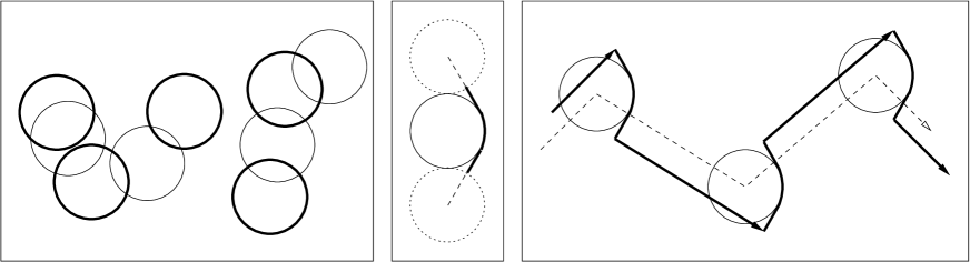
Figure 5: From left to right: (i) a line-sweep independent set (in bold lines); (ii) the curve $\gamma$; (iii) a part of the constructed disk tour.

Approximation algorithm—outline.

The idea is to first compute a maximal independent set and then an approximate tour of the centers of the independent set, as in [17]. The approximate tour of the centers is then extended by detours so that it visits all the other disks (not in the independent set). However the details differ significantly in both phases of the algorithm, in order to obtain a better approximation ratio: a monotone independent set is found, and a tailored visiting procedure is employed that takes advantage of the special form of the independent set.

Let $\mathcal{D}$ be a set of unit disks. First, compute a maximal independent set of disks $\mathcal{I}\subset\mathcal{D}$ by the following line-sweep algorithm. Select a leftmost disk $\omega\in\mathcal{D}$ and include it in $\mathcal{I}$. Remove from $\mathcal{D}$ all disks intersecting $\omega$. Repeat this selection step as long as $\mathcal{D}$ is non-empty.

We call $\mathcal{I}$ a line-sweep independent set or $x$-monotone independent set. Clearly, $\mathcal{I}$ is a maximal independent set in $\mathcal{D}$, that is, each disk in $\mathcal{D}\setminus\mathcal{I}$ intersects a disk in $\mathcal{I}$. Moreover, by construction, each disk in $\mathcal{D}\setminus\mathcal{I}$ intersects the right half-circle boundary of a disk in $\mathcal{I}$. Let $L^{*}={\rm len}({\rm OPT}(\mathcal{D}))$ and $L_{\mathcal{I}}^{*}={\rm len}({\rm OPT}(\mathcal{I}))$. Obviously, $L_{\mathcal{I}}^{*}\leq L^{*}$.

Algorithm.

The algorithm for computing a TSP tour of the disks is as follows. Compute a (maximal) line-sweep independent set $\mathcal{I}$; write $k=|\mathcal{I}|$. Next, compute $T_{\mathcal{I}}=o_{1}\ldots o_{k}$, an $\alpha$-approximate tour of the center points of disks in $\mathcal{I}$, for some constant $\alpha>1$. If we use the PTAS for Euclidean TSP [2, 39], for a given $0<\varepsilon<1/2$, we have $\alpha=1+\varepsilon$. If we use the approximation algorithm for metric TSP due to Christofides [11], we have $\alpha=1.5$.

Write $S_{\mathcal{I}}=\{o_{1},o_{2},\ldots,o_{k}\}$. For each disk $\omega\in\mathcal{I}$, let $\omega^{-}$ and $\omega^{+}$ be the two unit disks tangent to $\omega$ from below and from above, respectively. Let $o^{-}$ and $o^{+}$ be the centers of $\omega^{-}$ and $\omega^{+}$, respectively. See Fig. 5(ii). Let $\gamma(\omega)$ be the open curve obtained as follows: start with the tangent segment of positive slope from $o^{-}$ to $\omega$; concatenate the arc of $\omega$ subtending a center angle of $\pi/3$ and symmetric about the $x$-axis; concatenate the tangent segment of negative slope from $\omega$ to $o^{+}$. Now remove two unit segments, one from each endpoint of the curve obtained in the previous step. The resulting curve is $\gamma=\gamma(\omega)$. Observe that the open curve $\gamma(\omega)$ intersects any unit disk from $\mathcal{D}$ that intersects the right half-circle boundary of $\omega$ (this includes $\omega$ as well). Let $v$ denote the vertical segment connecting the endpoints of $\gamma$. It is easy to check that

$${\rm len}(\gamma) =2\left(\frac{\pi}{6}+2\cos\frac{\pi}{6}-1\right)=2\left(\frac{\pi}{6}+\sqrt{3}-1\right)\leq 2.512,$$

$${\rm len}(v) =4-\sqrt{3}\leq 2.268.$$ (19)

Replace each segment $o_{i}o_{i+1}$ of this tour, with $i$ odd, by a parallel segment of equal length connecting the two highest endpoints of the curves $\gamma(\omega_{i})$ and $\gamma(\omega_{i+1})$. Similarly, replace each segment $o_{i}o_{i+1}$ of this tour, with $i$ even, by a parallel segment of equal length connecting the two lowest endpoints of $\gamma(\omega_{i})$ and $\gamma(\omega_{i+1})$. See Fig. 5(iii).

To obtain a tour (closed curve) we visit the disks in $\mathcal{I}$ in the same order as $T_{\mathcal{I}}$. After each segment, the tour traverses the corresponding curve $\gamma(\omega)$ (going up or down, as needed, in an alternating fashion). If $k$ is even we proceed as above, while if $k$ is odd, the curve $\gamma(\omega_{1})$ is traversed in a circular way (going down along $\gamma$ and up again along the vertical segment $v$) in order to get a closed curve. We call $T$ the resulting tour.

Algorithm analysis.

Since any disk in $\mathcal{D}$ is either in $\mathcal{I}$ or intersects the curve $\gamma(\omega)$ of some disk $\omega\in\mathcal{I}$, and since $T$ visits all disks in $\mathcal{I}$ and contains the curves $\gamma(\omega)$ of all disks in $\mathcal{I}$, it follows that $T$ is a valid tour for all disks in $\mathcal{D}$. Further observe that the disjoint unit disks in $\mathcal{I}$ are contained in the figure $C=T^{*}_{\mathcal{I}}+B(2)$. By Lemma 8, $\pi|\mathcal{I}|\leq{\rm Area}(C)\leq 4\,{\rm len}(T^{*}_{\mathcal{I}})+4\pi$, hence

$$k=|\mathcal{I}|\leq\frac{4}{\pi}L^{*}_{\mathcal{I}}+4\leq\frac{4}{\pi}L^{*}+4.$$ (20)

The total length of the detours incurred by $T$ over all disks in $\mathcal{I}$ is $k\,{\rm len}(\gamma)$ when $k$ is even, and $k\,{\rm len}(\gamma)+{\rm len}(v)$ when $k$ is odd. Hence by (5.1) the length of the output tour is bounded from above as follows.

$$L\leq L_{S_{\mathcal{I}}}+k\,{\rm len}(\gamma)+{\rm len}(v)\leq L_{S_{\mathcal{I}}}+(2.512k+2.268).$$ (21)

Inequality (20) implies the following upper bound on the second term in (21).

$$2.512k+2.268\leq 2.512\left(\frac{4}{\pi}L^{*}+4\right)+2.268.$$ (22)

We next bound from above the first term in (21). The inequality (18) applied to $\mathcal{I}$ and $S_{\mathcal{I}}$ yields

$$L^{*}_{S_{\mathcal{I}}}\leq L^{*}_{\mathcal{I}}+2k.$$ (23)

Since the algorithm computes a $\alpha$-approximation of the optimal tour for the points in ${S_{\mathcal{I}}}$, by (20) we have

$$L_{S_{\mathcal{I}}} \leq\alpha L^{*}_{S_{\mathcal{I}}}\leq\alpha(L^{*}_{\mathcal{I}}+2k)\leq\alpha(L^{*}+2k)$$

$$\leq\alpha\left(L^{*}+2\left(\frac{4}{\pi}L^{*}+4\right)\right)$$

$$\leq\alpha\left(\left(1+\frac{8}{\pi}\right)L^{*}+8\right).$$ (24)

Substituting into (21) the upper bounds in (5.1) and (22) yields

$$L \leq\alpha\left(\left(1+\frac{8}{\pi}\right)L^{*}+8\right)+2.512\left(\frac{4}{\pi}L^{*}+4\right)+2.268$$

$$\leq\left(\alpha\left(1+\frac{8}{\pi}\right)+2.512\cdot\frac{4}{\pi}\right)L^{*}+(8\alpha+4\cdot 2.512+2.268)$$

$$\leq(3.5465\alpha+3.1984)L^{*}+(8\alpha+12.32).$$ (25)

For $\alpha=1+\varepsilon$ (using the PTAS for the center points), the length of the output tour is $L\leq 6.75\,L^{*}+20.4$, assuming that $\varepsilon\leq 0.001$. A more precise calculation along the lines above yields the following upper on the main term (in $L^{*}$); the constant factor appears in Theorem 3; note also that $1/0.53>1.8$, which explains the other parameter in Theorem 3.

$$\left(\frac{7}{3}+\frac{8\sqrt{3}}{\pi}\right)\left(1+\frac{\left(1+\frac{8}{\pi}\right)\varepsilon}{\left(\frac{7}{3}+\frac{8\sqrt{3}}{\pi}\right)}\right)L^{*}\leq\left(\frac{7}{3}+\frac{8\sqrt{3}}{\pi}\right)(1+0.53\,\varepsilon)L^{*}.$$

The running time is dominated by that of computing a $(1+\varepsilon)$-approximation of the optimal tour of $n$ points in $\mathbb{R}^{2}$.

For $\alpha=1.5$ (using the algorithm of Christofides for the center points), the length of the output tour is $L\leq 8.52\,L^{*}+24.4$. The running time is dominated by that of computing a minimum-length perfect matching on $n$ points in the plane ($n$ even), e.g., $O(n^{3/2}\log^{5}{n})$ by using the algorithm of Varadarajan [53].

Remarks.

1. If the input consists of pairwise-disjoint (unit) disks, then (5.1) yields improved approximations. These are not new: the case $\alpha=1+\varepsilon$ was already analyzed in [17]; we just list them for comparison. For $\alpha=1+\varepsilon$, (5.1) yields $L\leq 3.55\,L^{*}+8.01$, assuming that $\varepsilon\leq 0.001$. For $\alpha=1.5$, (5.1) yields $L\leq 5.32\,L^{*}+12$. The approximation ratio $3.55$ for disjoint unit disks is probably far from tight; the current best lower bound is $2$, see [17]. The example in [32, Fig. 4] is yet another instance with a ratio (lower bound) of $2$. Hence the approximation ratio $6.75$ for unit disks (which uses the above) is probably also far from tight.

2. A simple example shows that one cannot extend the above approach to disks of arbitrary radii. Let $x\geq 1$. See Fig. 6 (left) where $n=3$, and Fig. 6 (right) for its analogue with arbitrarily large $n$. Let $x\to\infty$ and $\varepsilon\to 0$.

(i) Suppose that we first compute a maximal independent set $\mathcal{I}$ in a greedy manner, by selecting disks in increasing order of their radii. Further suppose that we start by computing $T$, a constant approximation for the shortest TSP tour on $\mathcal{I}$, for instance by using the algorithm of de Berg et al. [12]; recall, this algorithm works with fat, disjoint regions. In some instances, no constant factor extension (by adding suitable detours to visit the remaining disks) exists. In Fig. 6 (left), ${\rm len}({\rm OPT}(\mathcal{I}))=2\varepsilon$, while ${\rm len}({\rm OPT})=4x$. Moreover, since $x\to\infty$, no asymptotic constant factor can be guaranteed by this approach; indeed, for any constants $\alpha,\beta$, there exists $x$ large enough, such that $\alpha\,2\varepsilon+\beta<4x$.

Figure 6: A set of three disks of radii $1$, $x$, and $x$, centered at $0$, $1+x+\varepsilon$ and $1+3x$ (left) and a set of $n$ disks, $n\geq 3$, of radii $1,\ldots,1$, $x$ and $x$ (right). A maximal independent set of disks (in bold) is shown for each case.

(ii) Suppose that we first compute a maximal line-sweep independent set, as in our algorithm for unit disks. The same example depicted in Fig. 6 (left) shows that no constant factor extension (by adding suitable detours to visit the remaining disks) exists. Moreover, as in (i), since $x\to\infty$, no asymptotic constant factor can be guaranteed by this approach.

3. Consider an algorithm that first computes a maximal independent set $\mathcal{I}$ of disks (according to some criterion), then computes a good approximate tour of the disks in $\mathcal{I}$, and then extends this tour with the boundary circles of the disks in $\mathcal{I}$ (in some way). Observe that the length of the overall detour incurred in this way is proportional to $\sum_{i\in\mathcal{I}}r_{i}$. The following claim (and example) shows a deeper cause for which this general approach does not give a constant approximation ratio; see also [18] for refinements of this inequality and other related results.

Claim. For every $M>0$, there exists a disk packing in the unit square $[0,1]^{2}$ with $\sum r_{i}\geq M$ and all disks tangent to the unit segment $[0,1]\times[0,0]$.

Proof.

We place disks in layers of decreasing radius. Each layer consists of congruent disks placed in blocks in between consecutive tangent disks of the previous layer, or in between a disk and a vertical side, as in Fig. 7.

Figure 7: The first two layers of an iterative construction: $k=1$ (left), and $k=2$ (right).

The first layer consists of $k$ disks of radius $1/(2k)$, for some $k\geq 1$. By choosing the radius of the disks in the next layer much smaller than the radius of the disks in the current layer, one can “cover” any prescribed large fraction $\rho<1$ of the length of the bottom side of the square by disks tangent to the bottom side of the square and having the sum of radii at least $\rho/2$. Consequently, by using sufficiently many layers, one can achieve $\sum r_{i}\geq M$, as required. ∎

5.2 Unit balls in $\mathbb{R}^{3}$: an improved approximation

We need an analogue of Lemma 8, specifically Lemma 9 below; its proof works in the same way. Let $B(x)$ denote a ball of radius $x$. Let $G=(V,E)$ be a connected geometric graph in $\mathbb{R}^{3}$ and let $L={\rm len}(G)$. Let $C$ be the set of points at distance at most $x$ from the edges and vertices of $G$. Equivalently, $C=G+B(x)$ is the Minkowski sum of $G$ and $B(x)$.

Lemma 9.

${\rm Vol}(C)\leq\pi x^{2}L+\frac{4\pi}{3}x^{3}$. This bound cannot be improved.

Let $\mathcal{D}$ be a set of unit balls (as input). As in the planar case, we compute a maximal independent set of disks $\mathcal{I}\subset\mathcal{D}$ by a plane-sweep algorithm. For convenience, we sweep a horizontal plane in the positive direction of the $z$-axis. We call $\mathcal{I}$ a plane-sweep independent set or $z$-monotone independent set.

The algorithm computes a tour of $\mathcal{D}$ as follows. First, compute a maximal $z$-monotone independent set $\mathcal{I}$; write $k=|\mathcal{I}|$. Next, compute $T_{\mathcal{I}}=o_{1}\ldots o_{k}$, an $\alpha$-approximate tour of the center points of the balls in $\mathcal{I}$, for some constant $\alpha>1$. Write $S_{\mathcal{I}}=\{o_{1},o_{2},\ldots,o_{k}\}$. For each ball $\omega\in\mathcal{I}$, let $\Gamma=\Gamma(\omega)$ be a discrete set of $28$ lattice points associated with $\omega$ (relative to its center). For describing this set we will assume for convenience that the center of $\omega$ is $(0,0,0)$. Let $a=1/\sqrt{3}$. $\Gamma$ contains $16$ points in the plane $z=a$ and $12$ points in the plane $z=3a$; see Fig. 8. Specifically,

$$\Gamma =\{(-3a,-3a,a),(-3a,-a,a),(-3a,a,a),(-3a,3a,a),$$

$$(-a,-3a,a),(-a,-a,a),(-a,a,a),(-a,3a,a),$$

$$(a,-3a,a),(a,-a,a),(a,a,a),(a,3a,a),$$

$$(3a,-3a,a),(3a,-a,a),(3a,a,a),(3a,3a,a)\}$$

$$\cup\{(-3a,-a,3a),(-3a,a,3a),(-a,-3a,3a),(-a,-a,3a),(-a,a,3a),(-a,3a,3a),$$

$$(a,-3a,3a),(a,-a,3a),(a,a,3a),(a,3a,3a),(3a,-a,3a),(3a,a,3a)\}.$$

One can check that the points in $\Gamma$ admit a Hamiltonian path in which each edge has length $2a$, say $\xi(\Gamma)=\gamma_{1},\gamma_{2},\ldots,\gamma_{28}$, starting at $\gamma_{1}=(-a,-3a,a)$ and ending at $\gamma_{28}=(-a,-3a,3a)$.

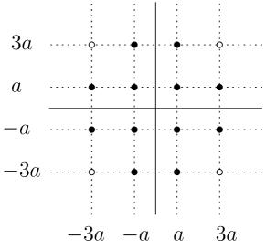
Figure 8: The set $\Gamma$ has $16$ points with $z=a$ and $12$ points with $z=3a$; $|\Gamma|=28$. The hollow circles indicate the four missing points in the plane $z=3a$.

We will prove shortly that any unit ball that intersects $\omega$ from above (i.e., the $z$-coordinate of its center is non-negative) contains at least one of the points in $\Gamma(\omega)$. Moreover, this also holds for $\omega$ itself.

We modify (extend) the tour $T_{\mathcal{I}}=o_{1}\ldots o_{k}$ as follows. Assume first that $k$ is even. We replace each segment $o_{i}o_{i+1}$ of this tour, with $i$ odd, by a parallel segment of equal length connecting $\gamma_{1}\in\Gamma(\omega_{i})$ with $\gamma_{1}\in\Gamma(\omega_{i+1})$. Similarly, we replace each segment $o_{i}o_{i+1}$ of this tour, with $i$ even, by a parallel segment of equal length connecting $\gamma_{28}\in\Gamma(\omega_{i})$ with $\gamma_{28}\in\Gamma(\omega_{i+1})$. To obtain a tour, we visit the balls in $\mathcal{I}$ in the same order as $T_{\mathcal{I}}$. After each segment, the tour visits all the $28$ points in the corresponding set $\Gamma(\omega)$ by using the Hamiltonian path $\xi(\Gamma)$ and then continues with the next segment, etc. This extension procedure can be adapted to work for odd $k$ without incurring any increase in cost: specifically, the first cycle of period $2$ is replaced by a cycle of period $3$. For odd $k$, the output TSP tour has the form $T=\xi_{1}\xi_{2}\xi_{3}\xi\xi^{R}\xi\xi^{R}\ldots\xi\xi^{R}$, rather than the form $T=\xi\xi^{R}\xi\xi^{R}\ldots\xi\xi^{R}$ (for $k$ even). Here $\xi^{R}$ is the path $\xi$ traversed in the opposite direction, and $\xi_{1},\xi_{2},\xi_{3}$ are three suitable Hamiltonian paths on $\Gamma$ (details are omitted).

Algorithm analysis.

The analysis of the approximation ratio is similar to that in the planar case. The disjoint unit balls in $\mathcal{I}$ are contained in the body $C=T^{*}_{\mathcal{I}}+B(2)$. By Lemma 9,

$$\frac{4\pi}{3}|\mathcal{I}|\leq{\rm Vol}(C)\leq 4\pi\,{\rm len}(T^{*}_{\mathcal{I}})+\frac{4\pi}{3}\,8,$$

hence

$$k=|\mathcal{I}|\leq 3\left(L^{*}+\frac{8}{3}\right)=3L^{*}+8.$$ (26)

The total length of the detours incurred by $T$ over all balls in $\mathcal{I}$ is bounded from above by

$$(28-1)2ak=27\frac{2}{\sqrt{3}}k=18\sqrt{3}k.$$ (27)

It follows that the length of the output tour is bounded from above as follows.

$$L\leq L_{S_{\mathcal{I}}}+18\sqrt{3}k.$$ (28)

The upper bound on $L_{S_{\mathcal{I}}}$ (analogue of (5.1)) is

$$L_{S_{\mathcal{I}}} \leq\alpha L^{*}_{S_{\mathcal{I}}}\leq\alpha(L^{*}_{\mathcal{I}}+2k)\leq\alpha(L^{*}+2k)\leq\alpha(L^{*}+2(3L^{*}+8))$$

$$=7\alpha L^{*}+16\alpha.$$ (29)

The upper bound on $18\sqrt{3}k$ (analogue of (22)) is

$$18\sqrt{3}k\leq 18\sqrt{3}(3L^{*}+8)=54\sqrt{3}L^{*}+144\sqrt{3}.$$ (30)

Substituting into (28) the upper bounds in (5.2) and (30) yields

$$L \leq(7\alpha L^{*}+16\alpha)+(54\sqrt{3}L^{*}+144\sqrt{3})$$

$$=(7\alpha+54\sqrt{3})L^{*}+(16\alpha+144\sqrt{3}).$$ (31)

For $\alpha=1+\varepsilon$ (using the PTAS for the center points), the length of the output tour is $L\leq 100.61\,L^{*}+265.6$, assuming that $\varepsilon\leq 0.01$. For $\alpha=1.5$ (using the algorithm of Christofides for the center points), the length of the output tour is $L\leq 104.1\,L^{*}+273.5$. The running time is dominated by that of computing a minimum-length perfect matching on $n$ points in $\mathbb{R}^{3}$ ($n$ even), e.g., $O(n^{3})$ [26].

Lemma 10.

Let $\omega$ and $\omega^{\prime}$ be two intersecting unit balls, centered at $(0,0,0)$ and $(x,y,z)$, respectively, where $z\geq 0$. Then $\omega$ contains a point in $\Gamma(\omega)$.

Proof.

By symmetry, it suffices to prove the claim when $x,y\geq 0$. We therefore have $x,y,z\geq 0$ and $x^{2}+y^{2}+z^{2}\leq 4$. We distinguish two cases, depending on whether $z\leq 2a$ or $z\geq 2a$. If $z\leq 2a$, we show that $\omega$ contains a point of $\Gamma$ in the lower plane $\sigma_{1}\ :\ z=a$; if $z\geq 2a$, we show that $\omega$ contains a point of $\Gamma$ in the higher plane $\sigma_{3}\ :\ z=3a$. Write $\Gamma_{1}=\Gamma\cap\sigma_{1}$, and $\Gamma_{3}=\Gamma\cap\sigma_{3}$.

Case 1: $z\leq 2a$. Since $x^{2}+y^{2}+z^{2}\leq 4$, we have $\max(x,y)\leq 2<4a$. The closest lattice point $\gamma=(\gamma_{x},\gamma_{y},\gamma_{z})\in\Gamma_{1}$ to $(x,y,z)$ satisfies

$$|x-\gamma_{x}|\leq a,\ \ |y-\gamma_{y}|\leq a,\ \ {\rm and}\ \ |z-\gamma_{z}|\leq a,$$

thus

$$(x-\gamma_{x})^{2}+(y-\gamma_{y})^{2}+(z-\gamma_{z})^{2}\leq 3a^{2}=1,$$

as required.

Case 2: $z\geq 2a$. Since $x^{2}+y^{2}+z^{2}\leq 4$, we have $x^{2}+y^{2}\leq 4-4a^{2}=8/3$. Observe that the disk $x^{2}+y^{2}\leq 8/3$ does not intersect the interior of the square $[2a,3a]^{2}$ in the plane $z=0$. Thus the projection of $(x,y,z)$ onto the plane $z=0$ is contained in $[0,3a]^{2}\setminus(2a,3a]^{2}$. This implies that the closest lattice point $\gamma=(\gamma_{x},\gamma_{y},\gamma_{z})\in\Gamma_{3}$ to $(x,y,z)$ satisfies

$$|x-\gamma_{x}|\leq a,\ \ |y-\gamma_{y}|\leq a,\ \ {\rm and}\ \ |z-\gamma_{z}|\leq a,$$

and the conclusion follows as in Case 1. ∎

Remark.

Analogous to the planar case, if the input consists of pairwise-disjoint (unit) balls, then (5.2) yields improved approximations. For $\alpha=1+\varepsilon$, (5.2) yields $L\leq 7.01\,L^{*}+16.1$, assuming that $\varepsilon\leq 0.001$. For $\alpha=1.5$, (5.2) yields $L\leq 10.5\,L^{*}+24$.

Generalization to higher dimensions.

The technique in this section generalizes to congruent balls in $\mathbb{R}^{d}$ for any fixed $d\geq 4$. First, the plane-sweep algorithm does so and yields an independent set $\mathcal{I}$. Then compute an $\alpha$-approximate tour $T_{\mathcal{I}}$ of the center points of the balls in $\mathcal{I}$ for a small $\alpha\leq 1.5$.

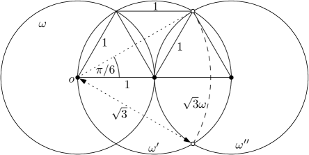
Figure 9: A unit disk $\omega$ centered at $o$ intersects two unit disks, $\omega^{\prime}$ and $\omega^{\prime\prime}$, whose centers are at distance 1 and 2 from $o$. Both $\omega^{\prime}$ and $\omega^{\prime\prime}$ intersects the boundary of $\sqrt{3}\omega$ in a spherical cap of radius $\sqrt{3}\cdot\pi/6$.

For each ball $\omega\in\mathcal{I}$, we construct a finite point set $\Gamma=\Gamma(\omega)$ with the property that any unit ball that intersects $\omega$ contains at least one of the points in $\Gamma(\omega)$. Consider a unit ball $\omega^{\prime}$ that intersects $\omega$. If the distance between their centers is less than 1, then $\omega^{\prime}$ contains the center of $\omega$; otherwise $\omega^{\prime}$ intersects the boundary of $\sqrt{3}\,\omega$ (i.e., the ball of radius $\sqrt{3}$ concentric with $\omega$) in a spherical cap of radius at least $\sqrt{3}\,\frac{\pi}{6}$ in spherical distance (refer to Fig. 9). The bound $\sqrt{3}\,\frac{\pi}{6}$ is attained when the centers of $\omega$ and $\omega^{\prime}$ are at distance 1 or 2 apart. Compute a maximal packing of the sphere $\partial(\sqrt{3}\omega)$ with spherical caps of radius $\sqrt{3}\,\frac{\pi}{12}$, starting with an arbitrary cap, and incrementally adding interior-disjoint caps so that each touches some previous cap.

Let $\Gamma(\omega)$ contain the centers of all caps in this maximal packing and the center of $\omega$. Suppose a unit disk $\omega^{\prime}$ intersects $\omega$ but misses $\Gamma(\omega)$. Then $\omega^{\prime}$ contains a spherical cap in $\partial(\sqrt{3}\omega)$ of radius at least $\sqrt{3}\cdot\pi/6$, which contains no point in $\Gamma(\omega)$; consequently a spherical cap with the same center and radius $\sqrt{3}\,\frac{\pi}{12}$ is disjoint from all caps in the packing, contradicting maximality. Therefore $\Gamma(\omega)$ has the desired property.

We extend the tour $T_{\mathcal{I}}$ by suitable detours visiting all points in $\Gamma(\omega)$ for all $\omega\in\mathcal{I}$ and thereby obtain a tour for the input set. The analysis of the approximation ratio is similar to the 2- and 3-dimensional cases and uses volume arguments in $\mathbb{R}^{d}$. Let ${\rm Vol}_{d}(r)$ be the volume of a ball of radius $r$ in $\mathbb{R}^{d}$. It is well-known that

$${\rm Vol}_{d}(r)=\begin{cases}\dfrac{\pi^{d/2}}{(d/2)!}\cdot r^{d}&{\rm if\ }d\ {\rm is\ even},\vskip 6.0pt plus 2.0pt minus 2.0pt\\ \dfrac{2^{d}\cdot\pi^{(d-1)/2}\,((d-1)/2)!}{d!}\cdot r^{d}&{\rm if\ }d\ {\rm is\ odd}.\end{cases}$$ (32)

Combining (32) with the Stirling formula yields the following upper bound:

Lemma 11.

$$\frac{{\rm Vol}_{d-1}(1)}{{\rm Vol}_{d}(1)}\leq(1+o(1))\sqrt{\frac{d}{2\pi}}.$$

Proof.

Write $f\sim g$ whenever $\lim_{d\to\infty}f(d)/g(d)=1$. We distinguish two cases according to the parity of $d$.

If $d$ is even, then

$$\frac{{\rm Vol}_{d-1}(1)}{{\rm Vol}_{d}(1)} = \frac{2^{d-1}\pi^{(d-2)/2}((d-2)/2)!}{(d-1)!}\frac{(d/2)!}{\pi^{d/2}}$$

$$= \frac{2^{d}}{\pi}\frac{\pi^{d/2}(d/2)!}{d!}\frac{(d/2)!}{\pi^{d/2}}\sim\frac{2^{d}}{\pi}\frac{(2\pi d/2)\left(\frac{d}{2e}\right)^{d}}{\sqrt{2\pi d}\left(\frac{d}{e}\right)^{d}}$$

$$= \frac{2^{d}}{\pi}\frac{\pi d}{\sqrt{2\pi d}}\frac{1}{2^{d}}=\sqrt{\frac{d}{2\pi}}.$$

If $d$ is odd, then

$$\frac{{\rm Vol}_{d-1}(1)}{{\rm Vol}_{d}(1)} = \frac{\pi^{(d-1)/2}}{((d-1)/2)!}\,\frac{d!}{2^{d}\pi^{(d-1)/2}\,((d-1)/2)!}$$

$$= \frac{d!}{2^{d}((d-1)/2)!((d-1)/2)!}\sim\frac{\sqrt{2\pi d}\left(\frac{d}{e}\right)^{d}}{2^{d}\,2\pi\frac{d-1}{2}\left(\frac{d-1}{2e}\right)^{d-1}}$$

$$= \frac{\sqrt{2\pi d}\,d^{d}\,2^{d-1}\,e^{d-1}}{\pi\,e^{d}\,2^{d}\,(d-1)^{d}}\sim\frac{\sqrt{2\pi d}}{2e\pi}\,e=\sqrt{\frac{d}{2\pi}}.$$

∎

By Lemma 11, a volume argument analogous to (26) yields

$$k=|\mathcal{I}|\leq\frac{{\rm Vol}_{d-1}(2)\,L^{*}+{\rm Vol}_{d}(2)}{{\rm Vol}_{d}(1)}\leq(1+o(1))\sqrt{\frac{d}{2\pi}}\,2^{d-1}L^{*}+2^{d}.$$

The surface area of a sphere of radius $r$ in $\mathbb{R}^{d}$ is ${\rm Area}_{d-1}(r)=2\pi r{\rm Vol}_{d-2}(r)$, and the surface area of a spherical cap of radius $r\varphi$ is bounded from below by ${\rm Vol}_{d-1}(r\sin\varphi)$. A volume argument yields

$$|\Gamma|\leq\frac{{\rm Area}_{d-1}(\sqrt{3})}{{\rm Vol}_{d-1}(\sqrt{3}\sin(\pi/12))}+1\leq\frac{2\pi{\rm Vol}_{d-2}(1)}{(\sin(\pi/12))^{d-1}{\rm Vol}_{d-1}(1)}+1\leq(1+o(1))\frac{\sqrt{2\pi d}}{(\sin(\pi/12))^{d-1}}.$$ (33)

If two spherical caps of radius $\sqrt{3}\,\frac{\pi}{12}$ are in contact on the sphere $\partial(\sqrt{3}\omega)$, then the distance between their centers is $2\sqrt{3}\sin\frac{\pi}{12}$. By construction, the length of a minimum spanning tree of $\Gamma$ is

$$(|\Gamma|-2)\,2\sqrt{3}\sin\frac{\pi}{12}+\sqrt{3}\leq(1+o(1))\frac{2\sqrt{6\pi d}}{(\sin(\pi/12))^{d-2}},$$

and the length of a Hamiltonian cycle $\xi$ of $\Gamma$ is at most twice this length. Consequently, we obtain a tour of length

$$L\leq\alpha L^{*}+2k\,{\rm len}(\xi)\leq\alpha L^{*}+2\left((1+o(1))\sqrt{\frac{d}{2\pi}}\,2^{d-1}L^{*}+2^{d}\right)\left((1+o(1))\frac{2\sqrt{6\pi d}}{(\sin(\pi/12))^{d-2}}\right).$$

The resulting (asymptotic) approximation ratio is

$$\alpha+(1+o(1))\frac{2\sqrt{3}\,d\,2^{d}}{(\sin(\pi/12))^{d-2}}=O\left(d\left(\frac{2}{\sin(\pi/12)}\right)^{d}\right)=O\left(7.73^{d}\right),$$

as claimed.

6 Conclusion

We revisited TSP with neighborhoods and obtained several approximation algorithms: some for neighborhoods previously less studied, such as lines and hyperplanes in $\mathbb{R}^{d}$, and some for the most previously studied, such as disks and balls. Despite the progress, one may rightfully say that the general problem of TSP with neighborhoods is far from resolved. Interesting questions remain open regarding the structure of optimal TSPN tours for lines, segments, balls, and hyperplanes, and the degree of approximation achievable for these problems. We record the simplest and most natural open questions on TSPN that we could identify.

• Is there a polynomial-time exact algorithm for planes in $\mathbb{R}^{3}$?

• Is there a constant approximation algorithm for lines in $\mathbb{R}^{3}$ (or in $\mathbb{R}^{d}$ for $d\geq 3$)? Can the current $O(\log^{3}n)$ ratio be improved?

• Is there a constant approximation algorithm for planar convex bodies?

• Is there a constant approximation algorithm for parallel segments in $\mathbb{R}^{3}$? To start with, one can further assume that the segments are pairwise-disjoint.

• Is there a constant approximation algorithm for balls (of arbitrary radii) in $\mathbb{R}^{3}$?

References

- [1] E. M. Arkin and R. Hasting, Approximation algorithms for the geometric covering salesman problem, Discrete Appl. Math. 55 (1994), 197–218.
- [2] S. Arora, Polynomial time approximation schemes for Euclidean traveling salesman and other geometric problems, Journal of the ACM 45(5) (1998), 753–782.
- [3] Y. Bartal, L.-A. Gottlieb, and R. Krauthgamer, The traveling salesman problem: low-dimensionality implies a polynomial time approximation scheme, in Proc. 44th Symposium on Theory of Computing (STOC), ACM Press, 2012, pp. 663–672.
- [4] M. Bern and D. Eppstein, Approximation algorithms for geometric problems, in Approximation Algorithms for NP-hard Problems (D. S. Hochbaum, ed.), PWS Publishing Company, Boston, MA, 1997, pp. 296–345.
- [5] M. Bern and P. Plassmann, The Steiner problem with edge lengths 1 and 2, Inform. Proc. Lett. 32 (1989), 171-–176.
- [6] H. L. Bodlaender, C. Feremans, A. Grigoriev, E. Penninkx, R. Sitters, and T. Wolle, On the minimum corridor connection problem and other generalized geometric problems, Comput. Geom. Theory Appl. 42(9) (2009), 939–951.
- [7] S. Carlsson, H. Jonsson and B. J. Nilsson, Finding the shortest watchman route in a simple polygon, Discrete & Computational Geometry 22(3) (1999), 377–402.
- [8] T.-H. H. Chan and K. Elbassioni, A QPTAS for TSP with fat weakly disjoint neighborhoods in doubling metrics, Discrete & Computational Geometry 46(4) (2011), 704–723.
- [9] T.-H. H. Chan and H.-C. Jiang, Reducing curse of dimensionality: improved PTAS for TSP (with neighborhoods) in doubling metrics, Proc. Symposium on Discrete Algorithms (SODA), 2016, to appear.
- [10] B. Chazelle and J. Matoušek, On linear-time deterministic algorithms for optimization problems in fixed dimension, J. Algorithms 21 (1996), 579–597.
- [11] N. Christofides, Worst-case analysis of a new heuristic for the traveling salesman problem, Technical Report 388, Graduate School of Industrial Administration, Carnegie-Mellon University, Pittsburg, 1976.
- [12] M. de Berg, J. Gudmundsson, M. J. Katz, C. Levcopoulos, M. H. Overmars, and A. F. van der Stappen, TSP with neighborhoods of varying size, Journal of Algorithms 57(1) (2005), 22–36.
- [13] M. Dror, A. Efrat, A. Lubiw, and J. S. B. Mitchell, Touring a sequence of polygons, in Proc. 35th Symposium on Theory of Computing, ACM Press, 2003, pp. 473–482.
- [14] M. Dror and J. B. Orlin, Combinatorial optimization with explicit delineation of the ground set by a collection of subsets, SIAM J. Discrete Math. 21(4) (2008), 1019–1034.
- [15] A. Dumitrescu, The traveling salesman problem for lines and rays in the plane, Discrete Mathematics, Algorithms and Applications 4(4) (2012), 1250044 (12 pages).
- [16] A. Dumitrescu and M. Jiang, Minimum-perimeter intersecting polygons, Algorithmica 63(3) (2012), 602–615.
- [17] A. Dumitrescu and J. S. B. Mitchell, Approximation algorithms for TSP with neighborhoods in the plane, Journal of Algorithms 48(1) (2003), 135–159.
- [18] A. Dumitrescu and Cs. D. Tóth, On the total perimeter of homothetic convex bodies in a convex container, Beiträge zur Algebra und Geometrie 56(2) (2015), 515–532.
- [19] A. Dumitrescu and Cs. D. Tóth, Constant-factor approximation for TSP with disks, preprint, October 2015, arxiv.org/abs/1506.07903.v2.
- [20] M. Dyer, N. Megiddo, and E. Welzl, Linear programming, Ch. 45 in Handbook of Discrete and Computational Geometry (J. E. Goodman and J. O’Rourke, eds.), CRC Press, 2004.
- [21] K. M. Elbassioni, A. V. Fishkin, N. H. Mustafa, and R. Sitters, Approximation algorithms for Euclidean group TSP, Proc. 32nd Internat. Colloq. Automata Lang. Prog. (ICALP), LNCS 3580, Springer, 2005, pp. 1115–1126.
- [22] K. M. Elbassioni, A. V. Fishkin, and R. Sitters, On approximating the TSP with intersecting neighborhoods, Proc. 17th Internat. Sympos. on Algorithms and Computation (ISAAC) LNCS 4288, Springer, 2006, pp. 213–222.
- [23] K. M. Elbassioni, A. V. Fishkin, and R. Sitters, Approximation algorithms for the Euclidean traveling salesman problem with discrete and continuous neighborhoods, Int. J. Comput. Geometry Appl. 19(2) (2009), 173–193.
- [24] J. Fakcharoenphol, S. Rao, and K. Talwar, A tight bound on approximating arbitrary metrics by tree metrics, J. Comput. Syst. Sci. 69(3) (2004), 485–497.
- [25] L. Few, The shortest path and shortest road through points, Mathematika 2 (1955), 141–144.
- [26] H. N. Gabow, An efficient implementation of Edmonds’ algorithm for maximum matchings on graphs, Journal of the ACM 23 (1976), 221–234.
- [27] M. R. Garey, R. Graham, and D. S. Johnson, Some NP-complete geometric problems, Proc. 8th Annual ACM Symposium on Theory of Computing (STOC), ACM Press, 1976, pp. 10–22.
- [28] M. R. Garey and D. S. Johnson: Computers and Intractability: A Guide to the Theory of NP-Completeness, W. H. Freeman and Company, New York, 1979.
- [29] N. Garg, G. Konjevod, and R. Ravi, A polylogarithmic approximation algorithm for the group Steiner tree problem, Journal of Algorithms 37(1) (2000), 66–84.
- [30] J. Gudmundsson and C. Levcopoulos, A fast approximation algorithm for TSP with neighborhoods, Nordic J. of Comput. 6 (1999), 469–488.
- [31] E. Halperin and R. Krauthgamer, Polylogarithmic inapproximability, in Proc. 35th ACM Symposium on Theory of Computing (STOC), ACM Press, 2003, pp. 585–594.
- [32] L. Häme, E. Hyytiä, and H. Hakula, The traveling salesman problem with differential neighborhoods, in Abstracts of the 27th European Workshop on Comput. Geom., Morschach, Switzerland, 2011, pp. 51–54.
- [33] H. Jonsson, The traveling salesman problem for lines in the plane, Inform. Proc. Lett. 82(3) (2002), 137–142.
- [34] C. Levcopoulos and A. Lingas, Bounds on the length of convex partitions of polygons, in Proc. 4th Conf. on Foundations of Software Technology and Theoretical Computer Science, LNCS 181, Springer, 1984, pp. 279–295.
- [35] C. Mata and J. S. B. Mitchell, Approximation algorithms for geometric tour and network design problems, Proc. 11th ACM Sympos. Comput. Geom. (SOCG), ACM Press, 1995, pp. 360–369.
- [36] J. Matoušek, M. Sharir, and E. Welzl, A subexponential bound for linear programming, Algorithmica 16 (1996), 498–516.
- [37] E. W. Mayr, H. J. Prömel, and A. Steger (editors), Lectures on Proof Verification and Approximation Algorithms, LNCS 1367, Springer, 1998.
- [38] N. Megiddo, Linear programming in linear time when the dimension is fixed, Journal of ACM 31 (1984), 114–127.
- [39] J. S. B. Mitchell, Guillotine subdivisions approximate polygonal subdivisions: A simple polynomial-time approximation scheme for geometric TSP, -MST, and related problems, SIAM J. on Comput. 28(4) (1999), 1298–1309.
- [40] J. S. B. Mitchell, Geometric shortest paths and network optimization, in Handbook of Computational Geometry (J.-R. Sack, J. Urrutia, eds.), Elsevier, 2000, pp. 633–701.
- [41] J. S. B. Mitchell, Shortest paths and networks, in Handbook of Computational Geometry (J. E. Goodman and J. O’Rourke, eds.), Chapman & Hall/CRC, 2004, pp. 607–641.
- [42] J. S. B. Mitchell, A PTAS for TSP with neighborhoods among fat regions in the plane, Proc. Symposium on Discrete Algorithms (SODA), ACM Press, 2007, pp. 11–18.
- [43] J. S. B. Mitchell, A constant-factor approximation algorithm for TSP with pairwise-disjoint connected neighborhoods in the plane, Proc. Symposium on Computational Geometry (SOCG), ACM Press, 2010, pp. 183–191.
- [44] C. H. Papadimitriou, Euclidean TSP is NP-complete, Theor. Comp. Sci. 4 (1977), 237–244.
- [45] F. P. Preparata and M. I. Shamos, Computational Geometry: An Introduction, Springer, New York, 1985.
- [46] S. B. Rao and W. D. Smith, Approximating geometrical graphs via “spanners” and “banyans”, Proc. 30th ACM Sympos. Theory Comput. (STOC) ACM Press, 1998, pp. 540–550.
- [47] G. Reich and P. Widmayer, Beyond Steiner’s problem: a VLSI oriented generalization, in Proc. Graph-Theoretic Concepts in Computer Science (WG), LNCS 411, 1990, Springer, pp. 196–-210.
- [48] S. Safra and O. Schwartz, On the complexity of approximating TSP with neighborhoods and related problems, Computational Complexity 14(4) (2005), 281–307.
- [49] P. Slavik, The errand scheduling problem, CSE Technical Report 97-02, University of Buffalo, Buffalo, NY1, 1997.
- [50] S. Spirkl, The guillotine subdivision approach for TSP with neighborhoods revisited, preprint, April 2014, arXiv:1312.0378v2.
- [51] X. Tan, T. Hirata and Y. Inagaki, Corrigendum to ‘An incremental algorithm for constructing shortest watchman routes’, Internat. J. Comput. Geom. Appl. 9(3) (1999), 319–323.
- [52] X. Tan, Fast computation of shortest watchman routes in simple polygons, Inform. Proc. Lett. 77(1) (2001), 27–33.
- [53] K. Varadarajan, A divide-and-conquer algorithm for min-cost perfect matching in the plane, Proc. 39th Sympos. Foundations of Comp. Sci. (FOCS) IEEE, 1998, pp. 320–331.