Double zigzag spin chain in strong magnetic field close to saturation

Abstract

We study the ground state phase diagram of a frustrated spin tube in a strong external magnetic field. This model can be viewed as two coupled zigzag spin chains, or as a two-leg spin ladder with frustrating next-nearest-neighbor couplings along the legs, and its study is motivated by the physics of such materials as Sulfolane-$\rm Cu_{2}Cl_{4}$ and $\rm BiCu_{2}PO_{6}$. In magnetic fields right below the saturation, the system can be effectively represented as a dilute gas of two species of bosonic quasiparticles that correspond to magnons with inequivalent incommensurate momenta at two degenerate minima of the magnon dispersion. Using the method previously proposed and tested for frustrated spin chains, we calculate effective interactions in this two-component Bose gas. On this basis, we establish the phase diagram of nearly-saturated frustrated spin tube, which is shown to include the two-component Luttinger liquid, two types of vector chiral phases, and phases whose physics is determined by the presence of bound magnons. We study the phase diagram of the model numerically by means of the density matrix renormalization group technique, and find a good agreement with our analytical predictions.

I Introduction

Frustrated spin systems, especially in low dimensions, display a rich variety of unconventionally ordered ground states Diep2004book ; Mila2011book . Strong external magnetic field, competing with the exchange interaction, can serve as a control parameter that drives the corresponding quantum phase transitions. The ground state of a frustrated quantum spin system is considerably simplified in a sufficiently strong external field that eventually leads to a fully polarized state above some critical field value $H_{s}$ (strictly speaking, the latter is true only for an axially-symmetric case, but we assume that deviations from axial symmetry are negligibly small). In fields just slightly below $H_{s}$, one may view the system as a dilute gas of excitations (magnons) on top of the fully polarized state BatyevBraginskii84 ; Johnson86 ; Gluzman94 ; NikuniShiba95 ; Okunishi98 ; JackeliZhitomirsky04 ; UedaTotsuka09 . At low density of magnons they can be approximately treated as bosonic quasiparticles. In the case of a strong frustration, the magnon dispersion has two or more degenerate minima at inequivalent incommensurate wave vectors, so one arrives at the picture of a multicomponent dilute Bose gas. In the one-dimensional case, infrared singularities, appearing in the description of effective interactions in the magnon gas, require special treatment Kolezhuk+12 .

Depending on the ratio of interactions between the same or different sorts of particles, several types of the ground state can be favored. Particularly, in two- and three-dimensional systems, different kinds of helical order (“fan” and “umbrella”) are realized NikuniShiba95 ; UedaTotsuka09 , while in one dimension quantum fluctuations destroy long-range helical order and may lead to the formation of several different states with competing types of unconventional short- and long-range orders. In one dimension, in the case of repulsion between magnons, the “umbrella” and “fan” phases get replaced by the vector chiral (VC) long-range order KV05 ; Mc+08 ; Okunishi08 ; KMc09 ; Hikihara+10 (which is equivalent to the local spin current) and by the two-component Tomonaga-Luttinger liquid (TLL2)Okunishi+99 , respectively. On the other hand, attraction between quasiparticles can lead to the appearance of a short-range multipolar (spin nematic) order Hikihara+08 ; Sudan+09 , or alternatively to metamagnetic jumps Arlego+11 .

Recently, the above approach, based on the mapping to the multicomponent Bose gas, has been successfully applied to spin-$S$ zigzag spin chain Arlego+11 ; Kolezhuk+12 , which is a paradigmatic model of a frustrated spin system. It has been shown that for zigzag chains close to saturation this approach is able to capture the physics of phase transitions between the VC and TLL2 phases, and for $S\geq 1$ it can detect the boundary of the (metamagnetic) region where bound states of magnons are formed. In the present paper, we employ this method to study the strong-field part of the ground state phase diagram of the frustrated spin tube shown in Fig. 1. The spin tube, which will be the subject of our study, can be viewed as two coupled zigzag spin chains, or as a two-leg spin ladder with frustrating next-nearest-neighbor couplings along the legs, see Fig. 1. This model is described by the following Hamiltonian:

$$\mathcal{H} = \sum_{n=1}^{L}\sum_{a=1,2}\Big{\{}J_{\perp}(\bm{S}_{n,1}\cdot\bm{S}_{n,2})-H(S_{n,1}^{z}+S_{n,2}^{z})$$

$$+ J_{1}(\bm{S}_{n,a}\cdot\bm{S}_{n+1,a})+J_{2}(\bm{S}_{n,a}\cdot\bm{S}_{n+2,a})\Big{\}},$$

where $\bm{S}_{n,a}$ are spin-$S$ operators acting at the $n$-th site of the $a$-th leg, $J_{1}$ and $J_{2}$ are the nearest-neighbor (NN) and next-nearest neighbor (NNN) exchange couplings along the legs, $J$ is the rung exchange, and $H$ is the external magnetic field. The system may be alternatively viewed as four antiferromagnetic chains connected by rung and zigzag couplings. This model has been recently studied at zero field VekuaHonecker06 ; Lavarelo+11 . It is believed to be relevant for the physics of such quasi-one-dimensional materials as Sulfolane-$Cu_{2}Cl_{4}$ ($\rm Cu_{2}Cl_{4}H_{8}C_{4}SO_{2}$) Fujisawa+03 , which exhibited unusual critical behavior in the field-induced transition from a helimagnetic to a non-magnetic phase Garlea+08 ; Garlea+09 ; Zheludev+09 , and $\rm BiCu_{2}PO_{6}$, which has attracted the attention of several research groups as being a realization of a frustrated ladder system with incommensurate correlations Koteswararao+07 ; Mentre+09 ; Tsirlin+10 . Apart from the possible relevance for the above materials, this model is fundamentally interesting since it presents the simplest example of two interacting zigzag chains.

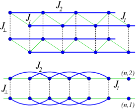
Figure 1: (Color online). The frustrated spin tube described by the Hamiltonian (I). The tube can be alternatively viewed as two zigzag chains coupled by the transversal interaction $J_{\perp}$, or as a spin ladder with next-nearest-neighbor exchange couplings along the legs (lower panel).

In this paper, we are interested in the frustrated case, so $J_{2}$ is chosen to be positive while $J_{1}$ may have any sign. It is convenient to use the quantity

$$\beta=J_{1}/J_{2}$$ (2)

as the frustration parameter. We will be interested in the regime $|\beta|<4$, when the magnon dispersion develops two degenerate minima at inequivalent points $\pm Q$ in the momentum space (in what follows, we refer to this regime as “strong frustration”).

For $S=\frac{1}{2}$, the phase diagram of the above model in the absence of the magnetic field has been studied numerically Lavarelo+11 and was found to contain the rung singlet and the columnar dimer phase. Earlier, a slightly different version of the model including exchange coupling along diagonals of the ladder has been investigated VekuaHonecker06 ; its phase diagram at zero field has been shown to contain the rung singlet phase, the Haldane phase, and two different columnar dimerized phases. The magnetic phase diagram of both versions of the model is at present unexplored.

We study the ground state of the strongly frustrated ($|\beta|<4$) spin-$S$ tube decribed by the Hamiltonian (I) in high magnetic fields in the immediate vicinity of saturation, for spin values $S=1$ and $S=\frac{1}{2}$. It is shown that the phase diagram contains the two-component Luttinger liquid, two types of vector chiral phases, and phases whose physics is determined by the presence of bound magnons. We compare our analytical predictions with the results of numerical simulations using the density matrix renormalization groupwhite92 ; schollwoeck05 (DMRG) technique. To that end, we compute the chirality correlation function and magnetization distribution as functions of $\beta$ at several values of $J_{\perp}$, at fixed magnetization close to saturation. We demonstrate that the DMRG results are in a good agreement with our theoretical predictions.

The structure of the paper is as follows: in Sect. II we describe the mapping of the spin tube problem to the dilute two-component lattice Bose gas and outline the main steps of computing effective interactions. Section III discusses the specific predictions of the theory for spin tubes with $S=\frac{1}{2}$ and $1$, while Sect. IV presents the results of numerical analysis and their comparison with analytical predictions. Finally, Sect. V contains a brief summary.

II Effective two-component Bose gas description of the spin tube

We intend to map the spin problem (I) to a dilute gas of interacting magnons, for values of the field $H$ slightly lower than the saturation field $H_{s}$. For that purpose, it is convenient to use the Dyson-Maleev representation for the spin operators in (I):

$$S_{nm}^{+}=\sqrt{2S}b_{nm},\quad S_{nm}^{-}=\sqrt{2S}b_{nm}^{{\dagger}}\Big{(}1-\frac{b_{nm}^{{\dagger}}b_{nm}^{\vphantom{{\dagger}}}}{2S}\Big{)},$$

$$S_{nm}^{z}=S-b_{nm}^{{\dagger}}b_{nm}^{\vphantom{{\dagger}}},$$ (3)

where $b_{nm}$ are bosonic operators acting at site $(nm)$ of the lattice, and $n=1,\ldots,L$ and $m=1,2$ denote the rung and leg numbers, respectively, see Fig. 1. To enforce the constraint $b_{nm}^{{\dagger}}b_{nm}^{\vphantom{{\dagger}}}\leq 2S$, one can add the infinite interaction term to the Hamiltonian, which reads:

$$\mathcal{H}\mapsto\mathcal{H}+U\sum_{nm}:(b_{nm}^{{\dagger}}b_{nm}^{\vphantom{{\dagger}}})^{2S+1}:\;,\quad U\to+\infty,$$ (4)

where $:(\ldots):$ denotes normal ordering. At the level of two-body interactions (which are dominating because of the diluteness of the gas) this term should be taken into account only for $S=\frac{1}{2}$.

Assuming periodic boundary conditions, we pass to the momentum representation for bosonic operators,

$$b_{nm}=\frac{1}{\sqrt{2L}}\sum_{\bm{k}}b_{\bm{k}}e^{ik_{x}n+k_{y}m},$$

where $\bm{k}=(k_{x},k_{y})$, with $k_{y}$ taking only values $0$ or $\pi$, and $L$ is the total number of rungs. Then one can cast the Hamiltonian (I) in the following form:

$$\mathcal{H}=\sum_{\bm{k}}E_{\bm{k}}b^{{\dagger}}_{\bm{k}}b_{\bm{k}}^{\vphantom{{\dagger}}}+\frac{1}{4L}\sum_{\bm{k}\bm{k^{\prime}}\bm{q}}V_{\bm{q}}(\bm{k},\bm{k^{\prime}})b^{{\dagger}}_{\bm{k}+\bm{q}}b^{{\dagger}}_{\bm{k^{\prime}}-\bm{q}}b_{\bm{k}}^{\vphantom{{\dagger}}}b_{\bm{k^{\prime}}}^{\vphantom{{\dagger}}}.$$ (5)

Here the magnon dispersion $E_{\bm{k}}$ is given by

$$E_{\bm{k}}=H-2(J_{1}+J_{2})S+2SJ_{k_{x}}+J_{\perp}S(\cos k_{y}-1),$$ (6)

where we use the shorthand notation

$$J_{k}\equiv J_{1}\cos(k)+J_{2}\cos(2k).$$ (7)

In the case of the strong frustration $|\beta|<4$, which is of main interest for us, there are two inequivalent degenerate minima of $E_{\bm{k}}$ that are reached at wave vectors $\bm{k}=(\pm Q,\pi)$ and $\bm{k}=(\pm Q,0)$ for positive and negative $J_{\perp}$, respectively. The wave vector $Q$ is incommensurate and is given by

$$Q=\arccos(-\beta/4).$$ (8)

The saturation field $H_{s}$ can be found noteHs from the condition $(\min\left.E_{\bm{k}})\right|_{H=H_{s}}=0$ :

$$H_{s}=2S\big{\{}J_{1}+J_{2}+J_{\perp}\theta(J_{\perp})-J_{Q}\big{\}},$$ (9)

where $\theta(x)$ is the Heaviside function. The external field may be viewed as playing the role of the chemical potential $\mu=H_{s}-H$ for magnons. In what follows, it is convenient to introduce instead of $E_{\bm{k}}$ the quantity

$$\varepsilon_{\bm{k}}=E_{\bm{k}}+\mu.$$ (10)

For $S\geq 1$, the two-body interaction $V_{\bm{q}}(\bm{k},\bm{k^{\prime}})$ depends on the transferred momentum $q$ as well as on the incoming momenta $k$, $k^{\prime}$:

$$V_{\bm{q}}(\bm{k},\bm{k^{\prime}}) = 2J_{q_{x}}-J_{k_{x}}-J_{k_{x}^{\prime}}$$

$$+ J_{\perp}\big{\{}\cos q_{y}-\frac{1}{2}(\cos k_{y}+\cos k_{y}^{\prime})\big{\}}.$$

For spin $\frac{1}{2}$, one has to add the term (4) to the Hamiltonian, simultaneously dropping the terms like $b_{nm}b_{nm}$ involving double occupancy. As a result, for $S=\frac{1}{2}$ the expression for the two-body interaction simplifies to

$$V_{\bm{q}}(\bm{k},\bm{k^{\prime}})=U+J_{\perp}\cos q_{y}+2J_{q_{x}},\quad U\to+\infty.$$ (12)

The model (5) describes two magnon branches of different parity with respect to the permutation of the ladder legs. We denote the operators describing even and odd magnons by $c_{k}$ and $a_{k}$, respectively:

$$a_{k}=b_{(k,\pi)},\quad c_{k}=b_{(k,0)}.$$ (13)

In this notation, the Hamiltonian takes the form

$$\mathcal{H} = \sum_{\bm{k}}\Big{\{}(\varepsilon_{k}^{a}-\mu)a^{{\dagger}}_{k}a_{k}^{\vphantom{{\dagger}}}+(\varepsilon_{k}^{c}-\mu)c^{{\dagger}}_{k}c_{k}^{\vphantom{{\dagger}}}\Big{\}}+\frac{1}{2L}\sum_{kk^{\prime}q}\Big{\{}V_{q}^{aa}(k,k^{\prime})a^{{\dagger}}_{k+q}a^{{\dagger}}_{k^{\prime}-q}a_{k}^{\vphantom{{\dagger}}}a_{k^{\prime}}^{\vphantom{{\dagger}}}+V_{q}^{cc}(k,k^{\prime})c^{{\dagger}}_{k+q}c^{{\dagger}}_{k^{\prime}-q}c_{k}^{\vphantom{{\dagger}}}c_{k^{\prime}}^{\vphantom{{\dagger}}}$$

$$+ V_{q}^{ac}(k,k^{\prime})a^{{\dagger}}_{k+q}a^{{\dagger}}_{k^{\prime}-q}c_{k}^{\vphantom{{\dagger}}}c_{k^{\prime}}^{\vphantom{{\dagger}}}+V_{q}^{ca}(k,k^{\prime})c^{{\dagger}}_{k+q}c^{{\dagger}}_{k^{\prime}-q}a_{k}^{\vphantom{{\dagger}}}a_{k^{\prime}}^{\vphantom{{\dagger}}}+V_{q}^{\times}(k,k^{\prime})c^{{\dagger}}_{k+q}a^{{\dagger}}_{k^{\prime}-q}c_{k}^{\vphantom{{\dagger}}}a_{k^{\prime}}^{\vphantom{{\dagger}}}\Big{\}},$$

The magnon energies and interaction amplitudes above can be read off Eqs. (6), (10), (II), (12). For the energies, one has

$$\varepsilon_{q}^{a}=2S(J_{q}-J_{Q}),\;\;\varepsilon_{q}^{c}=\varepsilon_{q}^{a}+2J_{\perp}S\quad\text{at $J_{\perp}>0$},$$ (14)

$$\varepsilon_{q}^{c}=2S(J_{q}-J_{Q}),\;\;\varepsilon_{q}^{a}=\varepsilon_{q}^{c}+2|J_{\perp}|S\quad\text{at $J_{\perp}<0$},$$

thus the energies of $a$-branch lie below (above) those of the $c$-branch for $J_{\perp}>0$ ($J_{\perp}<0$), respectively. When the magnetic field is decreased below $H_{s}$, the ground state of the system can be viewed as a dilute gas of $a$-magnons for $J_{\perp}>0$ or of $c$-magnons for $J_{\perp}<0$. Therefore, the last term in (II), describing the scattering of a $c$-magnon on an $a$-magnon, does not influence the structure of the ground state in the immediate vicinity of the saturation field: under the condition

$$\mu=H_{s}-H\ll\Delta_{1}\equiv 2SJ_{\perp}$$ (15)

(see Fig. 2) there is simply no regime when densities of both sorts of magnons ($a$ and $c$) are simultaneously nonzero. In what follows, we assume that the condition (15) is always satisfied, so we can safely ignore the presence of the last term in (II). However, the other amplitudes in (II), e.g., describing conversion of a pair of $a$-magnons to a pair of $c$-magnons, have to be kept, because they contribute to intermediate virtual states in multiple scattering processes.

The other two-body interaction amplitudes for $S\geq 1$ are

$$V_{q}^{cc}(k,k^{\prime})=V_{q}^{ca}(k,k^{\prime})=J_{q}-\frac{1}{2}(J_{k}+J_{k^{\prime}}),$$

$$V_{q}^{ac}(k,k^{\prime})=J_{q}-J_{\perp}-\frac{1}{2}(J_{k}+J_{k^{\prime}}),$$ (16)

$$V_{q}^{aa}(k,k^{\prime})=J_{q}+J_{\perp}-\frac{1}{2}(J_{k}+J_{k^{\prime}}),$$

and for $S=\frac{1}{2}$ they have to be modified as

$$V_{q}^{cc}=V_{q}^{aa}=\frac{1}{2}(U+J_{\perp})+J_{q},$$

$$V_{q}^{ac}=V_{q}^{ca}=\frac{1}{2}(U-J_{\perp})+J_{q}.$$ (17)

We have thus mapped the initial spin problem onto a 1d lattice gas of particles with a nontrivial double-minima dispersion. The renormalized two-body interaction in such a gas can be easily found in the dilute limit, i.e., $\mu\to 0$. Since the self-energy vanishes at $\mu\to 0$, the full propagator coincides with the bare one Uzunov81 , and thus the Bethe-Salpeter (BS) equation for the renormalized two-body interaction vertex $\Gamma_{q}^{\alpha\beta}(k,k^{\prime};E)$ (where $E$ is the total energy of the incoming particles) takes the following form:BatyevBraginskii84

$$\Gamma_{q}^{\alpha\beta}(k,k^{\prime};E)=V_{q}^{\alpha\beta}(k,k^{\prime})$$ (18)

$$\qquad-\frac{1}{L}\sum_{p}\sum_{\gamma}\frac{V_{q-p}^{\alpha\gamma}(k+p,k^{\prime}-p)\Gamma_{p}^{\gamma\beta}(k,k^{\prime};E)}{\varepsilon_{k+p}^{\gamma}+\varepsilon_{k^{\prime}-p}^{\gamma}-E},$$

where labels $\alpha$, $\beta$, $\gamma$ denote the magnon branch and can take the values “$a$” and “$c$”. The above equation is schematically shown in terms of Feynman diagrams in Fig. (3).

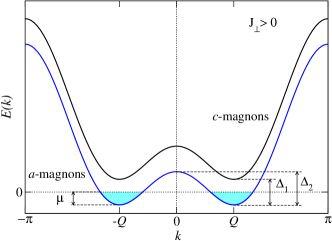
Figure 2: (Color online). Schematic picture of the magnon dispersion in the vicinity of the saturation field. For the sake of definiteness, the case of antiferromagnetic $J_{\perp}$ is shown. The system is populated by $a$-magnons with the momenta close to $\pm Q$, provided that the chemical potential $\mu=H_{s}-H$ satisfies the conditions (15) and (19).

If the magnetic field is close enough to the saturation, so that the condition

$$\mu=H_{s}-H\ll\Delta_{2}\equiv 2J_{2}S(|\beta|/4-1)^{2}$$ (19)

is satisfied (see Fig. 2), then the system is mainly populated by magnons (of $a$- or $c$-branch, depending on the sign of $J_{\perp}$) with momenta around the two dispersion minima at $\pm Q$, which at low energies can be interpreted as two different bosonic “flavors”. For those low-energy modes, one can formulate the effective theory in the form of the Gross-Pitaevsky-type energy functional for a two-component Bose field:

$$\mathcal{H}_{\rm GP} = \int dx\,\Big{\{}\sum_{\sigma=1,2}\frac{|\nabla\Phi^{\sigma}|^{2}}{2m}+\frac{1}{2}\Gamma_{11}(n_{1}^{2}+n_{2}^{2})$$ (20)

$$+ \Gamma_{12}n_{1}n_{2}-\mu(n_{1}+n_{2})\Big{\}}.$$

Here the Planck constant is set to unity, $\Phi^{1,2}$ are the macroscopic bosonic fields that describe magnons with momenta $k$ lying within the intervals $|k\pm Q|<\Lambda$ around the dispersion minima, $\Lambda$ is the infrared cutoff, $n_{\sigma}=|\Phi^{\sigma}|^{2}$ are the particle densities, and $m$ is the effective mass,

$$\frac{1}{m}=\left.\frac{\partial^{2}\varepsilon_{k}}{\partial k^{2}}\right|_{k=Q}=\frac{SJ_{2}(16-\beta^{2})}{2}.$$ (21)

The point $\Gamma_{11}=\Gamma_{12}$ corresponds to the enhanced $SU(2)$ symmetry at the level of the effective low-energy theory. For $\Gamma_{12}<\Gamma_{11}$, the ground state of the gas contains an equal density of the two particle species, and for $\Gamma_{12}>\Gamma_{11}$ just one of the two species is present in the ground state. In the spin problem the total number of each bosonic species is not separately fixed, in contrast to a typical setup for atomic mixtures. In a setup with fixed particle numbers, the ground state at $\Gamma_{12}<\Gamma_{11}$ is in the mixed phase, and $\Gamma_{12}>\Gamma_{11}$ corresponds to phase separation. In the spin language, the separated phase maps to the vector chiral (VC) phase KV05 , while the mixed phase corresponds to the two-component Tomonaga-Luttinger liquid (TLL2) FathLittlewood98 ; Okunishi+99 .

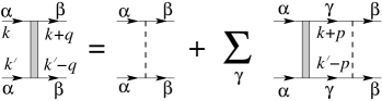
Figure 3: The ladder approximation to the Bethe-Salpeter equation for the renormalized two-body interaction vertex $\Gamma_{q}^{\beta\alpha}(k,k^{\prime};E)$. Solid lines denote bare propagators. The approximation becomes exact at $\mu\to 0$.

Macroscopic effective couplings $\Gamma_{11}$, $\Gamma_{12}$ of the Gross-Pitaevsky-type theory can be obtained from the $E\to 0$ limit of the corresponding vertex functions:

$$\Gamma_{11} = \left.\Gamma_{0}^{\alpha\alpha}(Q,Q;0)\right|_{\Lambda=\Lambda_{*}},$$

$$\Gamma_{12} = \left.\big{[}\Gamma_{0}^{\alpha\alpha}(-Q,Q;0)+\Gamma_{2Q}^{\alpha\alpha}(-Q,Q;0)\big{]}\right|_{\Lambda=\Lambda_{*}},$$ (22)

where $\alpha=$“$a$” or “$c$” for positive and negative $J_{\perp}$, respectively, and the vertex function $\Gamma_{q}^{\alpha\alpha}(k,k^{\prime};E)$ is the solution of the BS equation (18) with the infrared cutoff $|p|>\Lambda$ employed in the summation over internal transferred momenta $p$. The resulting expressions are viewed as functions of the running cutoff $\Lambda$ in the spirit of the renormalization group (RG) approach, and the RG flow $\Lambda\to 0$ is then interrupted at a certain scale $\Lambda=\Lambda_{*}=\sqrt{\mu m/2}$ that depends on the chemical potential (or, in other words, on the magnon density). The above approach is well known for one-component Bose gas FisherHohenberg88 ; NelsonSeung89 ; KolomeiskyStraley92 ; Kolomeisky+00 and has been successfully applied to the multicomponent case recently Kolezhuk10 ; Kolezhuk+12 .

There is an alternative approach Lee+02 ; Morgan+02 ; Kolezhuk+12 , which, instead of the infrared cutoff in the momentum space, introduces an “off-shell” regularization: the two-body scattering amplitudes in the presence of a finite particle density are obtained by taking the “bare” expressions $\Gamma_{q}^{\alpha\beta}(k,k^{\prime};E)$ at a finite negative energy $E=-E_{*}=-\pi^{2}\mu/8$:

$$\Gamma_{11} = \left.\Gamma_{0}^{\alpha\alpha}(Q,Q;-E_{*})\right|_{\Lambda=0},$$ (23)

$$\Gamma_{12} = \left.\big{[}\Gamma_{0}^{\alpha\alpha}(-Q,Q;-E_{*})+\Gamma_{2Q}^{\alpha\alpha}(-Q,Q;-E_{*})\big{]}\right|_{\Lambda=0},$$

where $\alpha$ takes the same value as in Eq. (II). One can show Kolezhuk+12 that the off-shell regularization yields the results that are equivalent to the cutoff regularization scheme. In this work, we have used the off-shell regularization because it is more convenient technically.

Our model contains only short-range interactions, so the solution of (18) can be expressed in terms of a finite number of Fourier modes in the transferred momentum BatyevBraginskii84 . In our case, from the structure of $V_{q}^{\alpha\beta}(k,k^{\prime})$ it is easy to see that each component of $\Gamma_{q}^{\alpha\beta}(k,k^{\prime};E)$ can contain only five Fourier harmonics proportional to $1$, $\cos q$, $\sin q$, $\cos 2q$, and $\sin 2q$. The system of integral equations is thus reduced to a system of linear equations that can be solved analytically for any value of the spin $S$.

For the purpose of finding only the Gross-Pitaevsky effective couplings $\Gamma_{11}$, $\Gamma_{12}$, the problem can be simplified even further. First of all, the system (18) describes four equations for the vertices, which split into two decoupled pairs: a pair of coupled equations for $\Gamma^{aa}$, $\Gamma^{ca}$, and another pair of coupled equations for $\Gamma^{cc}$ and $\Gamma^{ac}$. For $J_{\perp}>0$, the lowest energy excitations are $a$-magnons, and thus, in order to find the effective couplings $\Gamma_{11}$, $\Gamma_{12}$, we only need to solve the first pair of the BS equations for $\Gamma^{aa}$, $\Gamma^{ca}$; similarly, for $J_{\perp}<0$ we are interested only in the equations for $\Gamma^{cc}$ and $\Gamma^{ac}$. Second, it is easy to see that $\Gamma_{11}$ can be found as the $q=0$ value of $\Gamma^{\alpha\alpha}_{q}(Q,Q;-E_{*})$ which is an even function of the transferred momentum $q$, and $\Gamma_{12}$ may be represented as the $q=Q$ value of the function $\Gamma^{\alpha\alpha}_{Q+q}(-Q,Q;-E_{*})+\Gamma^{\alpha\alpha}_{Q-q}(-Q,Q;-E_{*})$, which is also even in $q$. For that reason, one can rewrite the integral equations (18) for the above two even functions, keeping only even Fourier harmonics UedaTotsuka09 . This reduces the number of resulting linear equations to six and makes the problem amenable to analytical treatment. We refer the reader to the Appendix for further details.

Solving the Bethe-Salpeter equation, one can show that the expansion of $\Gamma_{11}$, $\Gamma_{12}$ in $E_{*}$ has the following structure:Kolezhuk+12

$$\frac{1}{\Gamma_{11}} = \left(\frac{m}{4E_{*}}\right)^{1/2}+\frac{1}{g_{11}}+O(E_{*}^{1/2})+\ldots,$$

$$\frac{1}{\Gamma_{12}} = \left(\frac{m}{4E_{*}}\right)^{1/2}+\frac{1}{g_{12}}+O(E_{*}^{1/2})+\ldots$$ (24)

Note that for $E_{*}\to 0$ (i.e., $\mu\to 0$) the effective couplings $\Gamma_{11}$ and $\Gamma_{12}$ flow to the same value, which reflects the tendency of the RG flow to restore the $SU(2)$ symmetry for the two-component Bose mixture.Kolezhuk10

Parameters $g_{11}$, $g_{12}$, entering the second term in the expansions (II), under certain conditions, namely $|g_{11}|m\ll 1$ and $|g_{12}|m\ll 1$, can be identified with the effective bare coupling constants of the continuum two-component Bose gas with contact interactions (see Ref. Kolezhuk+12, for details). If the above conditions are broken, parameters $g_{ij}$ cannot be interpreted as physical bare couplings, and only the renormalized interactions $\Gamma_{ij}$ retain their meaning as effective low-energy coupling constants. The only physical meaning of $g_{ij}$ in such a case is that they are connected to the asymptotic phase shift of scattering states at small transferred momenta Kolezhuk+12 .

From Eqs. (II) one can see that transition points between the TLL2 and VC phases, that are determined by the condition $\Gamma_{11}=\Gamma_{12}$, correspond only to crossings of $g_{12}$ and $g_{11}$. (See, for example, Fig. 4a: when $g_{11}$ goes through a pole changing sign from plus to minus infinity, then at the pole $g_{12}-g_{11}$ changes sign from negative to positive, but this does not correspond to any phase transition, because on both sides of the pole in its immediate vicinity $\Gamma_{12}<\Gamma_{11}$).

Similarly, $g_{11}$ or $g_{12}$ becoming negative by going through a zero indicates the appearance of magnon bound states with zero total momentum, while a change of sign through a pole is not signaling any transition, but rather indicates a crossover into the so-called “super-Tonks” regime Astrakharchik-superTonks ; note-superTonks . It should be emphasized that within the present effective theory, which is essentially based on the two-body interaction, we cannot predict whether the formation of bound states stops at the level of bound magnon pairs, or continues with multiparticle bound states.

III Strong-field phase diagram: analytical results

Let us turn our attention to the specific predictions of our theory for the frustrated spin tube model defined by the Hamiltonian (I), at two spin values $S=1$ and $S=\frac{1}{2}$. Details concerning the solution of the BS equations can be found in the Appendix.

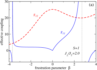
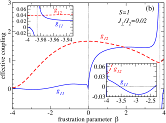
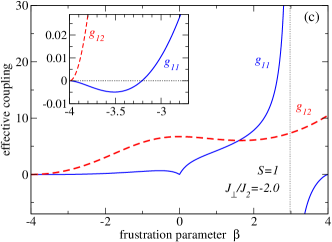
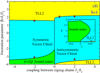
Figure 4: (Color online). (a) “Bare” coupling constants $g_{11}$, $g_{12}$ of the effective theory, obtained from the analytical solution of regularized Bethe-Salpeter equations, for $S=1$ frustrated spin tube with $J_{\perp}/J_{2}=2$; (b), (c) the same for $J_{\perp}/J_{2}=0.02$ and $J_{\perp}/J_{2}=-2$; (d) the predicted phase diagram in the vicinity of saturation; symbols show the transition points obtained from numerical simulations. Crossings of $g_{11}$ and $g_{12}$ correspond to transitions between the vector chiral and two-component Luttinger liquid phases, while the regions where $g_{11}$ becomes negative by going through a zero (not through a pole) indicate the appearance of magnon bound states.

Fig. 4a-c illustrates the behavior of the “bare” effective couplings $g_{11}$, $g_{12}$ for the spin-$1$ tube, as functions of the frustration parameter $\beta$, for several values of the interchain coupling $J_{\perp}$. VC-TLL2 transitions are detected by crossings of $g_{11}$ and $g_{12}$, and zeros of $g_{11}$ signal the formation of magnon bound states with the total momentum $k=\pm 2Q$. The resulting phase diagram is shown in Fig. 4d. One can see that the region of small $|\beta|$ always corresponds to the chiral phase, similar to the case of a single frustrated spin-$1$ chain Arlego+11 ; Kolezhuk+12 . For antiferromagnetic zigzag coupling $\beta>0$, there is only one transition between the vector chiral and the two-component Luttinger liquid phases, which is rather weakly dependent on the interchain (rung) coupling $J_{\perp}$. Nonanalytic behavior of the phase boundary at $J_{\perp}=0$ stems from the following: we assume that we work in the immediate vicinity of the saturation field (see conditions (15) and (19)), the ground state contains only $a$-magnons at $J_{\perp}>0$ and only $c$-magnons at $J_{\perp}<0$. It is clear that the magnetic field range, where the assumption (15) remains applicable, shrinks to zero as $J_{\perp}\to 0$, which causes the above nonanalyticity. At $J_{\perp}=0$ the model corresponds to two decoupled frustrated chains, so two magnon branches become degenerate, and the problem reduces to that for a single chain Kolezhuk+12 .

For ferromagnetic zigzag coupling $\beta<0$, there is a large region with negative $g_{11}$ supporting bound magnon states. From the numerical analysis for a single $S=1$ frustrated chain Arlego+11 , it is known that at least around $J_{\perp}=0$ there is a metamagnetic jump in the magnetization curves in this region. Presence of such a jump indicates formation of “magnon drops” – bound states of a large number of magnons. Increasing antiferromagnetic rung interaction $J_{\perp}>0$ leads to the opening of a finite TLL2 phase window close to $\beta=-4$ (which is the boundary of a transition into a one-component Luttinger liquid state).

Fig. 5 shows two examples of the characteristic behavior of the bare coupling, along with the resulting phase diagram, for the $S=\frac{1}{2}$ tube. The topology of the phase diagram is qualitatively the same as in the $S=1$ case, but there are certain caveats which one should have in mind. One important difference concerns the region of bound magnon states. It is known KuzianDrechsler07 that for a single isotropic $S=\frac{1}{2}$ frustrated chain with $\beta<0$ the lowest energy of a two-magnon bound state is not reached at the total momentum $k=\pm 2Q$, as one could expect from the picture of two bound magnons of the same flavor, but instead the minimum of the bound state dispersion lies at $k=\pi$ in a rather wide region of $-2.67<\beta<0$. For that reason, one may expect that the actual size of the region dominated by magnon bound states is larger than that of the region labeled “$k=2Q$ bound states” in Fig. 5. Second, from the analysis of the single-chain $S=\frac{1}{2}$ problem in Ref. Kolezhuk+12, , it is known that predictions of the present theory for the VC-TLL2 transition at $J_{\perp}=0$ should deviate substantially from the numerical results. In Section IV we will see, however, that agreement with the numerics is actually improved with the increase of the rung coupling strength $|J_{\perp}|$.

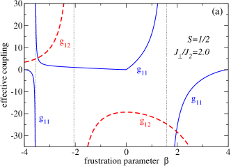
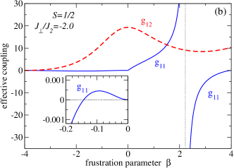
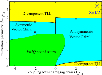
Figure 5: (Color online). “Bare” coupling constants $g_{11}$, $g_{12}$ for $S=\frac{1}{2}$ frustrated spin tube with (a) $J_{\perp}/J_{2}=2$ and (b) $J_{\perp}/J_{2}=-2$; (c) the predicted phase diagram in the vicinity of saturation, symbols show the transition points obtained from numerical simulations.

IV Numerical analysis

To verify our analytical predictions, we have studied the frustrated spin tube model (I) with $S=1$ and $S=\frac{1}{2}$ using the density matrix renormalization group white92 (DMRG) method (see Ref. schollwoeck05, for a detailed description of the DMRG technique).

We study the vector chirality correlation functions to identify the phases that have long-range vector chiral order. The ground state of spin tubes with $J_{\perp}>0$ near the saturation is populated with the magnons of the antisymmetric $a$-branch, so the relevant quantity in that case is the antisymmetric chirality

$$\bm{\kappa}_{A}(n)=(\bm{S}_{n,1}-\bm{S}_{n,2})\times(\bm{S}_{n+1,1}-\bm{S}_{n+1,2}).$$ (25)

Similarly, for $J_{\perp}<0$ one has to look at the correlators of the symmetric chirality

$$\bm{\kappa}_{S}(n)=(\bm{S}_{n,1}+\bm{S}_{n,2})\times(\bm{S}_{n+1,1}+\bm{S}_{n+1,2}).$$ (26)

In order to identify regions with metamagnetic behavior, i.e., the regions where magnon attraction leads to the formation of a single bound state consisting of a macroscopic number of magnons (“magnon drop”), we calculate the distribution of the rung magnetization $M_{n}=\langle S_{n,1}^{z}+S_{n,2}^{z}\rangle$ along the tube. This approach, however, does not allow to detect phases where the formation of bound states stops at the level of a finite number of magnons.

We use DMRG in its matrix product state formulation McCullochGulacsi02 ; McCulloch07 , which allows us to exploit the non-Abelian $SU(2)$ symmetry, as well as the Abelian $U(1)$. (While the magnetic field $H$ breaks $SU(2)$ symmetry, the fact that the Zeeman energy term commutes with the rest of the Hamiltonian makes it possible to take the influence of the magnetic field into account by calculating the ground state of the model in a sector with the given total spin $S_{\rm tot}$.) The advantage of using the $SU(2)$ symmetry lies in a considerable reduction of the number of states $m$ which is necessary to describe the system, because one essentially treats the multiplet of states of the same total spin as a single representative state.

The use of $SU(2)$ symmetry has a disadvantage as well: since the non-Abelian method allows to compute only reduced matrix elements (in the sense of the Wigner-Eckart theorem), one can only compute rotationally invariant correlators such as $\langle\bm{\kappa}_{A}(n)\cdot\bm{\kappa}_{A}(n^{\prime})\rangle$, etc. This can be inconvenient if the contribution of the transversal components of chirality exhibits strong oscillations that act as a “noise” masking the long-range order in the longitudinal component, as it has been found in frustrated chains McCulloch+08 . We have found such strong oscillations for $\bm{\kappa}_{S}$ in spin tubes with $J_{\perp}<0$, while the correlators of $\bm{\kappa}_{A}$ in $J_{\perp}>0$ systems were essentially free from oscillations. calculating

For that reason, we have used $SU(2)$ symmetry in our calculations for antiferromagnetically coupled tubes ($J_{\perp}>0$), and resorted to the standard $U(1)$ calculations for the $J_{\perp}<0$ case. Fig. 6 shows typical examples of chiral correlators for systems with ferro- and antiferromagnetic sign of $J_{\perp}$, calculated with or without the use of the $SU(2)$ symmetry.

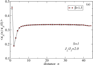
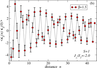
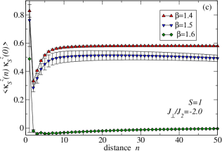
Figure 6: (Color online). Typical DMRG results for the chirality correlators of the $L=64$ spin-1 tube ($128$ spins) at the total magnetization $S_{\rm tot}=116$, inside the vector chiral phase: (a) rotationally invariant correlator of the antisymmetric chirality $\langle\bm{\kappa}_{A}(n)\cdot\bm{\kappa}_{A}(0)\rangle$, calculated with the use of the $SU(2)$ symmetry: there are no visible oscillations; (b) rotationally invariant correlator of the symmetric chirality $\langle\bm{\kappa}_{S}(n)\cdot\bm{\kappa}_{S}(0)\rangle$ exhibits strong oscillations which are due to the contribution of the transversal components as seen from (c) longitudinal correlators of the same quantity.

We have studied spin-$1$ and spin-$\frac{1}{2}$ spin tubes consisting of up to $256$ spins, with open boundary conditions, keeping up to $m=600$ states in most calculations. The total magnetization $M$ of the system has been set at about $90\%$ of the saturation value $M_{s}$ (specifically, we have kept $M/M_{s}=115/128$ for $S=1$ tubes and $M/M_{s}=29/32$ for $S=\frac{1}{2}$ ones). The (squared) chiral order parameters $\kappa_{A}^{2}$, $\kappa_{S}^{2}$ were extracted from the large-distance behavior of the corresponding correlation functions (the technicalities of this procedure are described in detail in Ref. Mc+08, ).

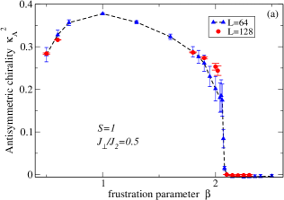
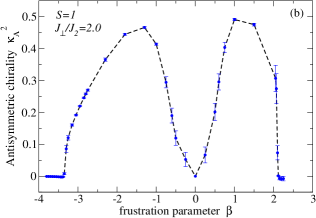
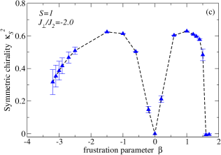
Figure 7: (Color online). Chirality order parameters of the $S=1$ tube obtained from the large-distance behavior of the correlation functions. The results for $L=64$ tube ($128$ spins) were calculated in the sector with the total spin $S_{\rm tot}=116$, and for $L=128$ we took $S_{\rm tot}=230$. (a) $J_{\perp}/J_{2}=0.5$; (b) $J_{\perp}/J_{2}=2.0$, only $L=64$ results are shown; (c) $J_{\perp}/J_{2}=-2.0$, here the calculations have been done using the usual $U(1)$ DMRG method for $L=128$ system. The point at $\beta=0$ has not been obtained numerically, but is included as a guide to the eye since the chirality must vanish at $\beta=0$.

Fig. 7 shows the behavior of the chiral order parameters along three constant-$J_{\perp}$ cuts in the phase diagram of the spin-$1$ tube. For antiferromagnetic rungs ($J_{\perp}/J_{2}=2$) one can clearly see two transitions around $\beta\approx 2.1$ and $\beta\approx-3.40$, which is consistent with the predictions of our theory (see Fig. 4d). At both transitions $\kappa_{A}$ vanishes in a rather abrupt manner, which suggests that the transition is of the first order. One can also notice that the amplitude of the chiral order decreases as $\beta$ tends to $0$, which is explained by the fact that at $\beta=0$ the chirality should vanish since this limit corresponds to two decoupled unfrustrated ladders.

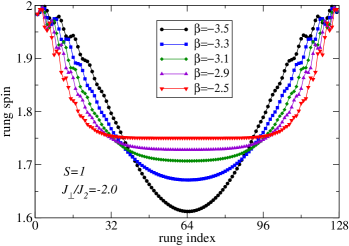
Figure 8: (Color online). The distribution of the rung magnetization $M_{n}=\langle S_{n,1}^{z}+S_{n,2}^{z}\rangle$ along the $S=1$ spin tube of the length $L=128$, at fixed $J_{\perp}/J_{2}=-2$ and several different values of the frustration parameter $\beta=J_{1}/J_{2}$ in the vicinity of the transition from the repulsive to the attractive magnon gas.

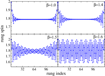
Figure 9: (Color online). The same as in Fig. 8, in the vicinity of the transition from the vector chiral into the two-component Tomonaga-Luttinger liquid phase.

For ferromagnetic rungs, $J_{\perp}/J_{2}=-2$, there is a transition in $\kappa_{S}$ at positive $\beta\approx 1.6$ which has a similar behavior to the corresponding transition in $\kappa_{A}$ at $J_{\perp}>0$, while the situation at negative $\beta$ is different: Looking simply at the chiral correlation functions, one tends to think that the chirality persists all the way up to $\beta=-4$, and merely the influence of the boundaries seems to increase considerably at $\beta\lesssim-3.0$. Fig. 8 shows how the distribution of the magnetization along the tube changes in this region of $\beta$. One can see that there is a transition at around $\beta\approx-3.2$ which corresponds to the formation of a macroscopic magnon “droplet” in the ground state, sitting in the middle of the system. This is exactly the behavior found in Ref. Arlego+11, for ferromagnetic frustrated $S=1$ chains, and indicates that the region with $\beta\lesssim-3.2$ exhibits a metamagnetic jump in the magnetization curve (the states with a “droplet” are never realized as true ground states at fixed magnetic field, they are only possible if the number of magnons is artificially fixed).

It is worthwhile to remark that the behavior of the magnetization distribution can be also used to detect the transition between the VC and TLL2 phases. Fig. 9 shows how the magnetization oscillations, which are localized at the boundaries in the VC phase, penetrate the bulk and spread over the entire system when one moves across the point $\beta\approx 1.5$. Comparing this behavior with Fig. 7c, one can see that $\beta\approx 1.5$ is indeed the transition point where the symmetric chirality vanishes.

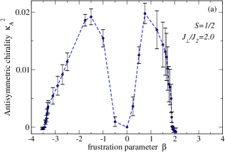
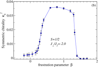
Figure 10: (Color online). Chirality order parameters of the $S=\frac{1}{2}$ tube extracted from the large-distance behavior of the correlation functions: (a) shows results obtained by means of the $SU(2)$-symmetric DMRG method for $L=64$ system ($128$ spins) with $J_{\perp}/J_{2}=2.0$, in the sector with the total spin $S_{\rm tot}=116$; the point at $\beta=0$ is included as a guide to the eye; (b) the results obtained by the standard $U(1)$-symmetric DMRG calculation for $L=128$ tube with $S_{\rm tot}=230$ and $J_{\perp}/J_{2}=-2.0$.

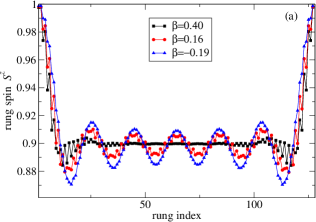
Figure 11: (Color online). (a) The distribution of the rung magnetization $M_{n}=\langle S_{n,1}^{z}+S_{n,2}^{z}\rangle$ along the $L=128$ spin-$\frac{1}{2}$ tube, at fixed $J_{\perp}/J_{2}=-2$ and several values of the frustration parameter $\beta$ in the vicinity of the transition from the vector chiral phase to the phase with bound magnons and dominating spin density wave correlations.

For $S=\frac{1}{2}$ tube, we have done similar calculations as for the spin-$1$ case, along two cuts at $J_{\perp}=\pm 2J_{2}$ in the phase diagram. The resulting behavior of the chiral order parameters along those lines is shown in Fig. 10. While at $J_{\perp}>0$ the picture is essentially similar to that for spin-$1$ system, as described above, at negative $J_{\perp}$ the transition at lower values of $\beta$ looks rather different: the chiral order parameter $\kappa_{S}$ disappears in a very smooth way, as seen from Fig. 10b (the corresponding correlation functions of the symmetric chirality are presented in Fig. 11b). At the same time, the distribution of magnetization at this transition shows the development of a spin density wave as seen in Fig. 11a. This is reminiscent of what happens in ferromagnetic frustrated spin chains Hikihara+08 ; Sudan+09 ; HM+09 , and indicates that this transition corresponds to the formation of bound states of finite number of magnons, in contrast to the $S=1$ case where there is a single bound state absorbing all the magnons present in the system.

Comparing our numerical results for the selected cuts in the phase diagram with the analytical predictions of the two-component Bose gas approach, one can see that our theory captures fairly well the physics of phase transitions in the frustrated spin tube model (I). Comparing the results for the $S=\frac{1}{2}$ spin tube (double zigzag chain) with those obtained by the same approach for single $S=\frac{1}{2}$ zigzag chain Kolezhuk+12 , one can see that the accuracy of the prediction for the VC-TLL2 transition is improved when one includes sufficiently strong rung coupling $|J_{\perp}|$. One obvious drawback of the theory, as mentioned at the end of Sect. III, is that it does not take into account the possibility to have the lowest energy of the bound state at the total momentum different from $\pm 2Q$, which is realized for $S=\frac{1}{2}$. We see that for that reason, our analytical predictions underestimate the size of the region dominated by bound states for $S=\frac{1}{2}$. Apart from that, one may call the agreement between the analytical theory and numerical simulations satisfactory.

V Summary

We study the ground state phase diagram of strongly frustrated four-leg spin-$S$ tube (which may be alternatively represented as two coupled zigzag spin chains, or as a two-leg spin ladder with next-nearest-neighbor couplings along the legs, see Fig. 1) in a strong magnetic field in the vicinity of saturation. The model is motivated by the physics of such frustrated quasi-one-dimensional spin-$\frac{1}{2}$ materials as Sulfolane-$\rm Cu_{2}Cl_{4}$ Fujisawa+03 ; Garlea+08 ; Garlea+09 ; Zheludev+09 and $\rm BiCu_{2}PO_{6}$Koteswararao+07 ; Mentre+09 ; Tsirlin+10 ; Lavarelo+11 , but is also interesting in itself as the simplest model of coupled frustrated chains. Although both in Sul-$\rm Cu_{2}Cl_{4}$ and $\rm BiCu_{2}PO_{6}$ the saturation field is too high to be accessible in current experiments, we hope that our findings, which establish the high-field slice of the phase diagram, will stimulate experimental studies of field-induced phases in those systems.

In the vicinity of saturation, the system can be represented as a dilute gas of two flavors of bosonic quasiparticles corresponding to magnons with momenta around two degenerate incommensurate minima of the magnon dispersion. Using the method previously proposed for frustrated spin chains Arlego+11 ; Kolezhuk+12 , we calculate effective interactions in this two-component Bose gas, and establish the high-field phase diagram of the frustrated spin tube. We show that the phase diagram contains two types of vector chiral phases (with symmetric and antisymmetric long-range chiral order), the two-component Luttinger liquid, and phases dominated by the presence of bound magnons.

We complement our analytical results by the numerical studies of $S=1$ and $S=\frac{1}{2}$ frustrated tubes by means of the density matrix renormalization group technique. We analyze the behavior of chiral correlation functions and distribution of the magnetization along several cuts in the phase diagram, and extract the position of the corresponding phase boundaries. The numerical results are found to be consistent with our analytical predictions.

*

Appendix A Computing the Gross-Pitaevsky couplings $\Gamma_{11}$, $\Gamma_{12}$

Consider in some detail the procedure of solving the Bethe-Salpeter equations (18). To reduce the number of Fourier harmonics, we first symmetrize the kernel. In doing so, we use the identities $\varepsilon_{k}^{\alpha}=\varepsilon_{-k}^{\alpha}$, $V_{q}^{\alpha\beta}(k,k^{\prime})=V_{-q}^{\alpha\beta}(k^{\prime},k)$, and $\Gamma_{q}^{\alpha\beta}(k,k^{\prime};E)=\Gamma_{-q}^{\alpha\beta}(k^{\prime},k;E)$. Let us introduce the following functions that are even in the transferred momentum $q$:

$$A_{q}^{\alpha\beta}\equiv\Gamma_{q}^{\alpha\beta}(Q,Q;-E_{*}),$$ (27)

$$B_{q}^{\alpha\beta}\equiv\Gamma_{Q+q}^{\alpha\beta}(-Q,Q;-E_{*})+\Gamma_{Q-q}^{\alpha\beta}(-Q,Q;-E_{*}),$$

then one has $\Gamma_{11}=A^{\alpha\alpha}(q=0)$ and $\Gamma_{12}(E)=B^{\alpha\alpha}(q=Q)$, with $\alpha=a$ for $J_{\perp}>0$ and $\alpha=c$ for $J_{\perp}<0$. One can rewrite Eqs. (18) as

$$A_{q}^{\alpha\beta} = u_{q}^{\alpha\beta}(0)-\frac{1}{L}\sum_{p}\sum_{\gamma}\frac{u_{q}^{\alpha\gamma}(p)A_{p}^{\gamma\beta}}{\varepsilon_{Q+p}^{\gamma}+\varepsilon_{Q-p}^{\gamma}+E_{*}},$$

$$B_{q}^{\alpha\beta} = v_{q}^{\alpha\beta}(Q)-\frac{1}{L}\sum_{p}\sum_{\gamma}\frac{v_{q}^{\alpha\gamma}(p)B_{p}^{\gamma\beta}}{2\varepsilon_{p}^{\gamma}+E_{*}},$$ (28)

where symmetrized kernels $u_{q}^{\alpha\beta}(p)$, $v_{q}^{\alpha\beta}(p)$ are even functions of $p$:

$$u_{q}^{\alpha\beta}(p)=\frac{1}{2}\big{\{}V^{\alpha\beta}_{q-p}(Q+p,Q-p)+V^{\alpha\beta}_{q+p}(Q-p,Q+p)\big{\}},$$

$$v_{q}^{\alpha\beta}(p)=\frac{1}{2}\big{\{}V^{\alpha\beta}_{p+q}(-p,p)+V^{\alpha\beta}_{p-q}(-p,p)\big{\}}.$$ (29)

Assume for definiteness that $J_{\perp}>0$, then of eight equations (A) we need only a pair of equations for $A_{q}^{aa}$ and $A_{q}^{ca}$, and another pair of equations for $B_{q}^{aa}$ and $B_{q}^{ca}$. Solutions to those equations can be now sought in the form containing only even Fourier harmonics:

$$A^{aa}_{q}=x_{0}+x_{1}\cos q+x_{2}\cos 2q,$$

$$A^{ca}_{q}=y_{0}+y_{1}\cos q+y_{2}\cos 2q,$$

$$B^{aa}_{q}=\widetilde{x}_{0}+\widetilde{x}_{1}\cos q+\widetilde{x}_{2}\cos 2q,$$ (30)

$$B^{ca}_{q}=\widetilde{y}_{0}+\widetilde{y}_{1}\cos q+\widetilde{y}_{2}\cos 2q.$$

This ansatz transforms each of the above pairs of the integral equations into a system of 6 linear equations for 6 variables. However, it follows from those equations that

$$y_{1}=x_{1},\quad\widetilde{y}_{1}=\widetilde{x}_{1},\quad y_{2}=x_{2},\quad\widetilde{y}_{2}=\widetilde{x}_{2},$$ (31)

so the size of the corresponding linear problems reduces to $4\times 4$. For $S=\frac{1}{2}$, one has to perform the limit $U\to+\infty$. After solving the linear systems, one can read off the effective couplings

$$\Gamma_{11}=x_{0}+x_{1}+x_{2},\quad\Gamma_{12}=\widetilde{x}_{0}-\frac{\beta}{4}\widetilde{x}_{1}+\big{(}\frac{\beta^{2}}{8}-1\big{)}\widetilde{x}_{2}.$$ (32)

The procedure for $J_{\perp}<0$ follows Eqs. (A)-(32), with the obvious interchange $a\leftrightarrow c$ of the magnon branch labels. Below we list the equations for $x_{i}$, $y_{i}$, $\widetilde{x}_{i}$, $\widetilde{y}_{i}$ in the form that is valid for any sign of $J_{\perp}$ as well as for any value of $S$, including $S=\frac{1}{2}$. The resulting systems of equations can be cast into the following form:

$$\begin{pmatrix}\frac{1}{J_{\perp}}+I_{11}^{b}&-\frac{1}{J_{\perp}}-I_{11}^{t}&I_{12}^{b}-I_{12}^{t}&I_{13}^{b}-I_{13}^{t}\\[5.69054pt] \frac{1-1/(2S)}{|J_{\perp}|-2J_{Q}}+I_{11}^{b}&\frac{1-1/(2S)}{|J_{\perp}|-2J_{Q}}+I_{11}^{t}&I_{12}^{b}+I_{12}^{t}&I_{13}^{b}+I_{13}^{t}\\[5.69054pt] I_{12}^{b}&I_{12}^{t}&\frac{1}{J_{1}}+I_{22}^{b}+I_{22}^{t}&I_{23}^{b}+I_{23}^{t}\\[5.69054pt] I_{13}^{b}&I_{13}^{t}&I_{23}^{b}+I_{23}^{t}&\frac{1}{J_{2}}+I_{33}^{b}+I_{33}^{t}\end{pmatrix}\begin{pmatrix}x_{0}\\[5.69054pt] y_{0}\\[5.69054pt] x_{1}\\[5.69054pt] x_{2}\end{pmatrix}=\begin{pmatrix}1\\[5.69054pt] 1\\[5.69054pt] 1\\[5.69054pt] 1\end{pmatrix},$$ (33)

$$\begin{pmatrix}\frac{1}{J_{\perp}}+\widetilde{I}_{11}^{b}&-\frac{1}{J_{\perp}}-\widetilde{I}_{11}^{t}&\widetilde{I}_{12}^{b}-\widetilde{I}_{12}^{t}&\widetilde{I}_{13}^{b}-\widetilde{I}_{13}^{t}\\[5.69054pt] \frac{1-1/(2S)}{|J_{\perp}|-2J_{Q}}+\widetilde{I}_{11}^{b}&\frac{1-1/(2S)}{|J_{\perp}|-2J_{Q}}+\widetilde{I}_{11}^{t}&\widetilde{I}_{12}^{b}+\widetilde{I}_{12}^{t}&\widetilde{I}_{13}^{b}+\widetilde{I}_{13}^{t}\\[5.69054pt] \widetilde{I}_{12}^{b}&\widetilde{I}_{12}^{t}&\frac{1}{J_{1}}+\widetilde{I}_{22}^{b}+\widetilde{I}_{22}^{t}&\widetilde{I}_{23}^{b}+\widetilde{I}_{23}^{t}\\[5.69054pt] \widetilde{I}_{13}^{b}&\widetilde{I}_{13}^{t}&I_{23}^{b}+I_{23}^{t}&\frac{1}{J_{2}}+\widetilde{I}_{33}^{b}+\widetilde{I}_{33}^{t}\end{pmatrix}\begin{pmatrix}\widetilde{x}_{0}\\[5.69054pt] \widetilde{y}_{0}\\[5.69054pt] \widetilde{x}_{1}\\[5.69054pt] \widetilde{x}_{2}\end{pmatrix}=\begin{pmatrix}2\\[5.69054pt] 2\\[5.69054pt] 2\cos Q\\[5.69054pt] 2\cos 2Q\end{pmatrix}$$ (34)

where the matrix coefficients are given by

$$I_{ij}^{b}=\frac{1}{\pi}\int_{0}^{\pi}\frac{f_{i}f_{j}}{2S(J_{Q+p}+J_{Q-p}-2J_{Q})+E_{*}},\quad I_{ij}^{t}=\frac{1}{\pi}\int_{0}^{\pi}\frac{f_{i}f_{j}}{2S(J_{Q+p}+J_{Q-p}+2|J_{\perp}|-2J_{Q})+E_{*}},$$

$$\widetilde{I}_{ij}^{b}=\frac{1}{\pi}\int_{0}^{\pi}\frac{f_{i}f_{j}}{4S(J_{p}-J_{Q})+E_{*}},\quad\widetilde{I}_{ij}^{t}=\frac{1}{\pi}\int_{0}^{\pi}\frac{f_{i}f_{j}}{4S(|J_{\perp}|+J_{p}-J_{Q})+E_{*}},$$

$$f_{1}=1,\quad f_{2}=\cos p,\quad f_{3}=\cos 2p,$$ (35)

and can all be computed analytically in a closed, though somewhat cumbersome, form. The solutions for $\Gamma_{11}$, $\Gamma_{12}$, which follow from Eqs. (33), (34), can be obtained with the help of any good computer algebra system (we used Maple), but are too bulky to be presented here (the result, saved in a plain ASCII format, is several megabytes large).

References

- (1) Frustrated Spin Systems, ed. by H.T. Diep (World Scientific, 2004).
- (2) Introduction to Frustrated Magnetism: Materials, Experiments, Theory, ed. by C. Lacroix, P. Mendels, and F. Mila (Springer Series in Solid-State Sciences 164, 2011).
- (3) E. G. Batyev and L. S. Braginskii, Zh. Eksp. Teor. Fiz. 87, 1361 (1984) [Sov. Phys. JETP 60(4), 781 (1984)].
- (4) M. D. Johnson and M. Fowler, Phys. Rev. B 34, 1728 (1986).
- (5) S. Gluzman, Phys. Rev. B 50, 6264 (1994).
- (6) T. Nikuni and H. Shiba, J. Phys. Soc. Japan 64, 3471 (1995).
- (7) K. Okunishi, Y. Hieida, and Y. Akutsu, Phys. Rev B. 59 6806 (1999).
- (8) G. Jackeli and M. E. Zhitomirsky, Phys. Rev. Lett. 93, 017201 (2004).
- (9) H. T. Ueda and K. Totsuka, Phys. Rev. B 80, 014417 (2009).
- (10) A. K. Kolezhuk, F. Heidrich-Meisner, S. Greschner, and T. Vekua, Phys. Rev. B 85, 064420 (2012).
- (11) A. Kolezhuk and T. Vekua, Phys. Rev. B 72, 094424 (2005).
- (12) I. P. McCulloch, R. Kube, M. Kurz, A. Kleine, U. Schollwöck, and A. K. Kolezhuk, Phys. Rev. B 77, 094404 (2008).
- (13) K. Okunishi, J. Phys. Soc. Japan 77, 114004 (2008).
- (14) A. K. Kolezhuk and I. P. McCulloch, Condensed Matter Physics 12, 429 (2009).
- (15) T. Hikihara, T. Momoi, A. Furusaki, and H. Kawamura, Phys. Rev. B 81, 224433 (2010).
- (16) K. Okunishi, Y. Hieida, and Y. Akutsu, Phys. Rev. B 60, R6953 (1999).
- (17) T. Hikihara, L. Kecke, T. Momoi, and A. Furusaki, Phys. Rev. B 78, 144404 (2008).
- (18) J. Sudan, A. Lüscher, and A. M. Läuchli, Phys. Rev. B 80, 140402(R) (2009).
- (19) M. Arlego, F. Heidrich-Meisner, A. Honecker, G. Rossini, and T. Vekua, Phys. Rev. B 84, 224409 (2011).
- (20) T. Vekua and A. Honecker, Phys. Rev. B 73, 214427 (2006).
- (21) A. Lavarélo, G. Roux, and N. Laflorencie, Phys. Rev. B 84, 144407 (2011).
- (22) M. Fujisawa, J.-I. Yamaura, H. Tanaka, H. Kageyama, Y. Narumi, and K. Kindo, J. Phys. Soc. Japan 72, 694 (2003).
- (23) V. O. Garlea, A. Zheludev, L.-P. Regnault, J.-H. Chung, Y. Qiu, M. Boehm, K. Habicht, and M. Meissner, Phys.Rev. Lett. 100, 037206 (2008).
- (24) V. O. Garlea, A. Zheludev, K. Habicht, M. Meissner, B. Grenier, L.-P. Regnault, and E. Ressouche, Phys. Rev. B 79, 060404(R) (2009).
- (25) A. Zheludev, V. O. Garlea, A. Tsvelik, L.-P. Regnault, K. Habicht, K. Kiefer, and B. Roessli, Phys.Rev. B 80, 214413 (2009).
- (26) B. Koteswararao, S. Salunke, A. V. Mahajan, I. Dasgupta, and J. Bobroff, Phys. Rev. B 76, 052402 (2007).
- (27) O. Mentré, E. Janod, P. Rabu, M. Hennion, F. Leclercq-Hugeux, J. Kang, C. Lee, M.-H. Whangbo, and S. Petit, Phys. Rev. B 80, 180413 (2009).
- (28) A. A. Tsirlin, I. Rousochatzakis, D. Kasinathan, O. Janson, R. Nath, F. Weickert, C. Geibel, A. M. Läuchli, and H. Rosner, Phys. Rev. B 82, 144426 (2010).
- (29) S. R. White, Phys. Rev. Lett. 69, 2863 (1992); Phys. Rev. B 48, 10 345 (1993).
- (30) U. Schollwöck, Rev. Mod. Phys. 77, 259 (2005).
- (31) The expression (9) is valid if there are no magnon bound states, otherwise the actual saturation field will differ from this value by the magnon binding energy.
- (32) D. Uzunov, Phys. Lett. A87, 11 (1981).
- (33) G. Fáth and P. B. Littlewood, Phys. Rev. B 58, R14709 (1998).
- (34) D. S. Fisher and P. C. Hohenberg, Phys. Rev. B 37, 4936 (1988).
- (35) D. R. Nelson and H. S. Seung, Phys. Rev. B 39, 9153 (1989).
- (36) E. B. Kolomeisky and J. P. Straley, Phys. Rev. B 46, 11749 (1992).
- (37) E. B. Kolomeisky, T. J. Newman, J. P. Straley, and X. Qi, Phys. Rev. Lett. 85, 1146 (2000).
- (38) A. K. Kolezhuk, Phys. Rev. A 81, 013601 (2010).
- (39) M. D. Lee, S. A. Morgan, M. J. Davis, and K. Burnett, Phys. Rev. A 65, 043617 (2002); see also arXiv:cond-mat/0305416 (unpublished).
- (40) S. A. Morgan, M. D. Lee, and K. Burnett, Phys. Rev. A 65, 022706 (2002).
- (41) G.E. Astrakharchik, D. Blume, S. Giorgini, and B.E. Granger, Phys. Rev. Lett. 92, 030402 (2004); M.T. Batchelor, M. Bortz, X.W. Guan, and N. Oelkers, J. Stat. Mech. L10001 (2005); G.E. Astrakharchik, J. Boronat, J. Casulleras, and S. Giorgini, Phys. Rev. Lett. 95, 190407 (2005).
- (42) The effective continuum theory in the strong coupling regime , does not fit into the description in terms of the repulsive Lieb-Liniger model, but rather corresponds to the so-called “super Tonks” Bose gas Astrakharchik-superTonks with the Luttinger parameter . The interested reader is referred to Ref. Kolezhuk+12, for further discussion.
- (43) R. O. Kuzian and S.-L. Drechsler, Phys. Rev. B 75, 024401 (2007).
- (44) I. P. McCulloch and M. Gulacsi, Europhys. Lett. 57, 852 (2002).
- (45) I. P. McCulloch, J. Stat. Mech.: Theor. Exp., P10014 (2007).
- (46) I. P. McCulloch, R. Kube, M. Kurz, A. Kleine, U. Schollwöck, and A. K. Kolezhuk, Phys. Rev. B 77, 094404 (2008).
- (47) F. Heidrich-Meisner, I. P. McCulloch, and A. K. Kolezhuk, Phys. Rev. B 80, 144417 (2009); ibid. 81, 179902 (2010).