The Asymmetric Pupil Fourier Wavefront Sensor

Abstract

This paper introduces a novel wavefront sensing approach that relies on the Fourier analysis of a single conventional direct image. In the high Strehl ratio regime, the relation between the phase measured in the Fourier plane and the wavefront errors in the pupil can be linearized, as was shown in a previous work that introduced the notion of generalized closure-phase, or kernel-phase. The technique, to be usable as presented requires two conditions to be met: (1) the wavefront errors must be kept small (of the order of one radian or less) and (2) the pupil must include some asymmetry, that can be introduced with a mask, for the problem to become solvable. Simulations show that this asymmetric pupil Fourier wavefront sensing or APF-WFS technique can improve the Strehl ratio from 50 to over 90 % in just a few iterations, with excellent photon noise sensitivity properties, suggesting that on-sky close loop APF-WFS is possible with an extreme adaptive optics system.

1 Non-common path error and extreme AO

Contrast limits for the direct imaging of extrasolar planets from ground based adaptive optics (AO) observations are currently set by the presence of static and slow-varying aberrations in the optical path that leads to the science instrument (Marois et al., 2003). Because some of these aberrations are not sensed by the wavefront sensor, something called the non-common path error, they are responsible for the presence of long lasting speckles in the image. Since extrasolar planets are faint unresolved sources, it is impossible to discriminate them among these speckles in one single frame. The family of differential imaging techniques is aimed at calibrating out some of these static aberrations, in post processing by using either sky rotation (angular differential imaging, or ADI), polarization differential imaging (PDI), or wavelength dependence of the speckles (spectral differential imaging or SDI). Of these, ADI Marois et al. (2006) has been successful in most notably producing the image of the planetary system around HR 8799 (Marois et al., 2008).

A new generation of high contrast instruments using an approach of improved wavefront control called extreme adaptive optics (XAO), aims at producing higher contrast raw images, by including additional high density wavefront control devices, fed by advanced wavefront sensing techniques to actively control the wavefront during the observations. In all cases, the primary goal of the high order deformable mirror is to calibrate the non-common path error between the conventional AO system and the science camera, and then to try and help creating a high contrast region in the image, by actively modulating the speckles in the field, for instance using speckle nulling (Martinache et al., 2012).

The control of the non common path error is an important element of any XAO system, that requires the implementation of dedicated hardware or special acquisition procedures: the Gemini Planet Imager (Wallace et al., 2010) and the Project P1640 (Zhai et al., 2012) for instance, both include a dedicated interferometric calibration unit, to characterize and compensate the non-common path error. Other options often involve some form of phase diversity, using multiple acquisitions with the science camera while moving an internal calibration source along the optical path with ESO’s SPHERE (Sauvage et al., 2010) and JPL’s PALM-3000 (Bouchez et al., 2010) or even the science camera itself with Subaru’s SCExAO project (Martinache et al., 2011).

This paper introduces an alternate approach to the calibration of the non common path error in XAO systems, using a non-invasive conventional hard-stop mask located in the pupil plane, and the direct analysis of the Fourier properties of the resulting images acquired with the focal plane camera. The simulations presented in this work demonstrate remarkable performance of the approach: combined with proper control of a deformable mirror (DM) that is present in all XAO system, it can bring the wavefront quality from a starting Strehl ratio of 50 % up to over 95 % in less than five iterations. Because of the mask’s very limited impact on the overall morphology of the point spread function (PSF) and its high sensitivity, the technique seems compatible with a general purpose imaging (non-coronagraphic) instrument, and would enable continuous tracking of the non-common path aberrations, to maintain very high Strehl during observation.

2 Wavefront Sensing in the Fourier-plane

Even in near-perfect observing conditions, diffraction is a significant hindrance to the interpretation of images at the highest angular resolution. In this diffraction-limited regime, it is advantageous to adopt an interferometric point of view of image formation, and work not from images directly, but from their Fourier Transform counterpart instead. Working on the Fourier Transform of images is often refered to as working in the Fourier-plane, the spatial-frequency plane or the uv-plane, the latter expression being widely used in sparse aperture interferometry. The Fourier Transform being a complex function, encodes information both in terms of amplitude (or modulus) and phase: this paper focuses solely on the phase.

To introduce the notion of kernel-phase, Martinache (2010) proposes a simple but powerful description of how pupil phase errors propagate into phase signal measured in the Fourier-plane, in terms of linear algebra. This model, when it applies (when wavefront errors are small i.e. $\varphi<1$ radian for a conventional imaging telescope), offers an interesting alternative to the traditional object-image relation, written in terms of convolution. When this model applies, the (usually unknown) instrumental phase in the pupil $\varphi$ can be related to the phases $\Phi$ measured in the Fourier plane with a single, fully determined, linear operator called the phase transfer matrix (noted $\mathbf{A}$). The discrete model, presented in several references (Martinache, 2010, 2011, 2012) is briefly re-introduced here for convenience.

The aperture of any instrument, usually refered to as the pupil, can be discretized into a finite collection of $n$ elementary sub-apertures, using a regular grid (for instance square or hexagonal) adapted to the actual pupil shape. One of these elementary sub-apertures is taken as a zero-phase reference: the pupil phase of a coherent point source is therefore written as a $(n-1)$-component vector $\varphi$, measured relative to this reference. Assuming that the image produced by the system is at least Nyquist-sampled, in the Fourier-plane, one is able to sample up to $m$ phases, organized in a vector $\Phi$.

The complete model (Martinache, 2010), also includes one additional term $\Phi_{0}$, that encodes the true phase information about the target of interest. The Fourier-phase $\Phi$ therefore writes as:

$$\Phi=\Phi_{0}+\mathbf{A}\cdot\varphi.$$ (1)

The motivation for this paper is to use this formalism not to learn something about the target, which was shown to be recoverable using kernel-phases, but to solve the wavefront sensing problem. This paper will therefore from now on consider the target to be a non-resolved source, so that $\Phi_{0}$ = 0. XAO systems typically include a laser-fed single-mode fiber calibration source, for off-line tests of wavefront control loops, that can be used in this purpose.

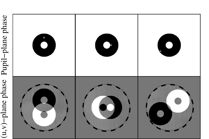
Figure 1: Illustration of the pupil phase propagation mechanism into phase measured in the Fourier plane. The top row shows a pupil phase “poke” applied to three different sub-apertures of the full two-dimensional pupil, in this case, a circular aperture with a 30 % central obscuration. The bottom row shows for each case the corresponding distribution of phase that is observed in the Fourier plane. The overlaid dashed-line circle in the bottom row marks the cutoff spatial frequency of the transfer function.

Wavefront sensing in the Fourier-plane is routinely achieved in long baseline interferometry. However, to be able to handle the large optical path differences (OPD) expected along a long baseline that can be up to several hundred meters long in the optical, resulting in phase shifts larger than $2\pi$, the strategy is to disperse the light so as to increase the coherence length and solve the $2\pi$ wrapping of the phase (Michelson & Pease, 1921; Koechlin et al., 1996). This strategy, so far only used with a small number of apertures was generalized by Martinache (2004), for a all in one Fizeau-type interferometer: an approach called “dispersed-speckles”. This approach appears as an relevant solution for the calibration of OPD inside AO fed integral field spectrographs (Peters et al., 2012). In systems where the OPD is small ($\sim$1 radian), dispersion isn’t necessary, and the use of a single wavelength may suffice in solving the problem.

This approach however has one major flaw: for a pupil like the one shown in Fig. 1, it is insensitive to structures of the wavefront that are even, that is for which $\varphi(-r)=\varphi(r)$. While an analytical demonstration of this fundamental property is provided in an appendix to the paper, one can build a more intuitive understanding of wavefront sensing in the Fourier plane, by considering the following scenarios, that illustrate how instrumental (pupil) phase errors $\varphi$ propagate into phase measured in the Fourier plane:

• If the phase is constant across the entire pupil, then none of the baselines formed by any pair of elementary sub-apertures does record a phase difference, and the phase in the Fourier plane is zero everywhere: the non-common path error is perfectly calibrated.

• If a phase offset $\delta_{0}$ is added to one single sub-element of the aperture, something we will refer to a ”poke”, then each baseline involving this sub-element records a phase difference, which is exactly $\pm\delta_{0}$. Fig. 1 presents several such scenarios.

• If the pupil-plane phase error $\varphi$ is completely random, each of the samples in the Fourier plane is then the average of $\mathbf{R}$ phase differences on the pupil, where $\mathbf{R}$ is a vector summarizing the redundancy of the baselines identified in the system.

To see that this approach to wavefront sensing would be insensitive to an even aberration, the reader can consider either of the scenarios shown in Fig. 1, and observe that the phase pattern recorded in the uv-plane for either of these “pokes” is perfectly odd: $\Phi(-r)=-\Phi(r)$, a property expected to the fact that it results from the Fourier Transform of a real image.

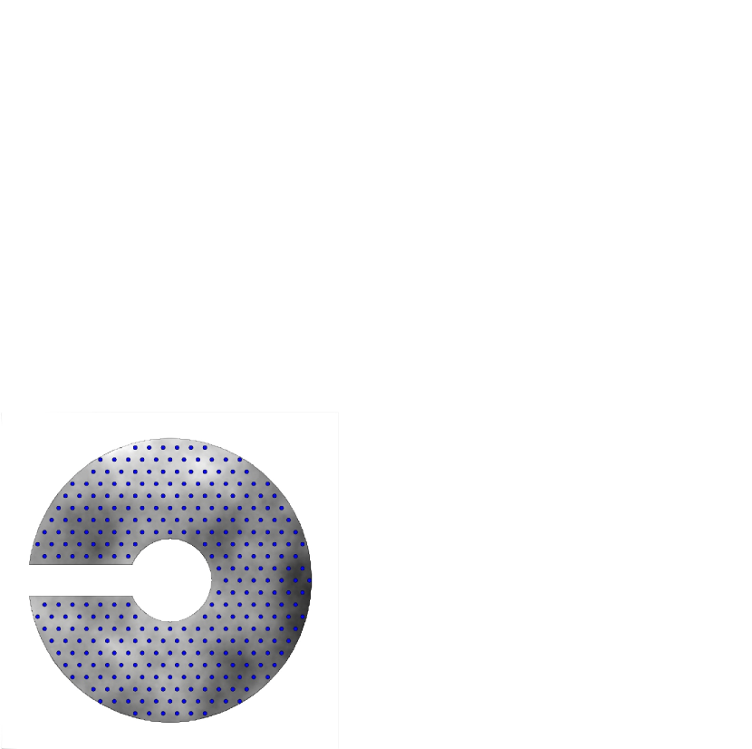
Figure 2: Discrete hexagonal model used to construct the phase transfer matrix $\mathbf{A}$. Each of the thick dots overlaying the ”true” image of the input pupil phase inside the asymmetric pupil, marks the location of a discrete pupil sample. This model contains 309 distinct pupil sample points.

If the same amplitude “poke” $\delta_{0}$ is applied to the diametrically opposed sub-aperture in the same direction (therefore creating an elementary even aberration), the two resulting phase patterns in the Fourier-plane will simply add to zero, and give the illusion that that the system is perfectly in phase, no matter what the amplitude of the “poke”. One equivalent way to say it is that such a Fourier-based wavefront sensor is only sensitive to the odd component of the input wavefront.

One simple way to circumvent this severe limitation is to introduce some asymmetry in the system, and the simplest thing to alter is the pupil. High contrast instruments are usually equiped with a multi-slot pupil wheel (ie. for coronagraphic Lyot-stops), and for this work, we propose to modify the pupil used in Fig. 1 by adding one single fairly thick spider arm that connects the outer edge of the pupil to the edge of the central obstruction. The actual pupil used for the results presented in this work is shown in Fig. 2.

3 Asymmetric Pupil Fourier Wavefront Sensor

We need to go back to the instrumental phase propagation model given summarized by eq. 1, to see how the asymmetry introduced in the pupil affects the properties of the phase transfer matrix $\mathbf{A}$. To build the actual matrix, the pupil is modeled into a discrete grid of sub-apertures that follow a regular hexagonal grid. Other options (eg. square grid) remain possible, and have been used so far for kernel-phase analysis (Martinache, 2010; Pope et al., 2012). The density of the grid should in practice be matched to the density of actuators the deformable mirror that controls the incoming wavefront. The image is expected to be at least Nyquist-sampled.

Without the missing sub-apertures along the thick arm, the model would contain $n_{a}=330$ pupil samples, propagating into $n_{uv}=708$ distinct samples in the Fourier-plane. Just like for the kernel-phase, the proposed analysis relies on the spectral properties of the phase transfer matrix $\mathbf{A}$. The singular value decomposition (SVD) of the $708\times 330$ resulting phase transfer matrix $\mathbf{A}$, given by:

$$\mathbf{A}=\mathbf{U}\cdot\mathbf{\Sigma}\cdot\mathbf{V^{T}},$$ (2)

where $\mathbf{U}$ and $\mathbf{V^{T}}$ are unitary matrices and $\mathbf{\Sigma}$ is a diagonal matrix containing the singular values of $\mathbf{A}$, reveals that for this symmetrical geometry, 165 (that is exactly $n_{a}/2$) of the singular values of $\mathbf{A}$ are non-zero. Using this knowledge, it therefore appears possible to build a pseudo-inverse for $\mathbf{A}$ that will enable the recovery of one half of the wavefront phase in the input pupil. This observation made after examination of the singular values of the phase transfer matrix, echoes the conclusion made in Sec. 2, that a Fourier based WFS can only sense the odd component of the input wavefront, in terms of linear algebra.

With the asymmetric pupil presented in Fig. 2, things apparently change very little: the number of apertures in the pupil may drop to 309 (a loss of 21 apertures), they still project onto the same space of 708 samples in the Fourier-plane, because of the redundance. However, a major change occurs in terms of spectral properties of this new phase transfer matrix. The SVD of the now $708\times 308$ linear operator reveals that all the required 308 singular values are now non-zero. A pseudo-inverse for $\mathbf{A}$ for such a configuration therefore enables full recovery of both odd and even parts of the wavefront.

In practice, the approach is used as follows: assuming that the residual aberrations on the wavefront are of the order of one radian or less (RMS), one asymmetric mask such as the one shown in Fig. 2 is introduced in the pupil of the instrument, before the final focal plane, while shining a calibration source (often a laser-fed single mode fiber). With nothing else being actuated, one (or more) image is acquired with the science detector, which will be assumed to be Nyquist sampled.

The data reduction procedure is very similar to what has been described for non-redundant masking interferometry data (Kraus et al., 2008) and kernel-phase data analysis (Martinache, 2010). Each image is simply recentered, and and multiplied by a window function to limit sensitivity to readout noise and filter out the spatial frequency content of the image that is beyond the control region of the wavefront control device. A Fourier transform for each image is then calculated, and the phase of this Fourier transform is sampled according to the discrete model described in Section 2. The resulting vector $\Phi$ is then simply projected back onto pupil phase $\varphi$ inside the region unocculted by the mask, using the pseudo inverse of $\mathbf{A}$.

4 APF-WFS performance

4.1 SVD modes for the APF-WFS

The wavefront reconstruction by the APF-WFS relies upon the determination of singular value modes of the phase transfer matrix that in turn solely depend on the geometry of the pupil sampling. The modes, which form an orthonormal basis for the wavefront, are also sorted in order of decreasing level of significance, proportional to their associated singular value.

Fig. 3 shows the first 30 modes (out of the total 309) the SVD of the phase transfer matrix produces. One will observe that although they do not closely match a familiar pattern of modes like the Zernike polynomials or the series of sines and cosines, the lower spatial frequencies (slope and curvature) are naturally reconstructed first, and higher spatial frequency content appears as the order of the modes increases, guided by the hexagonal geometry chosen to model the pupil.

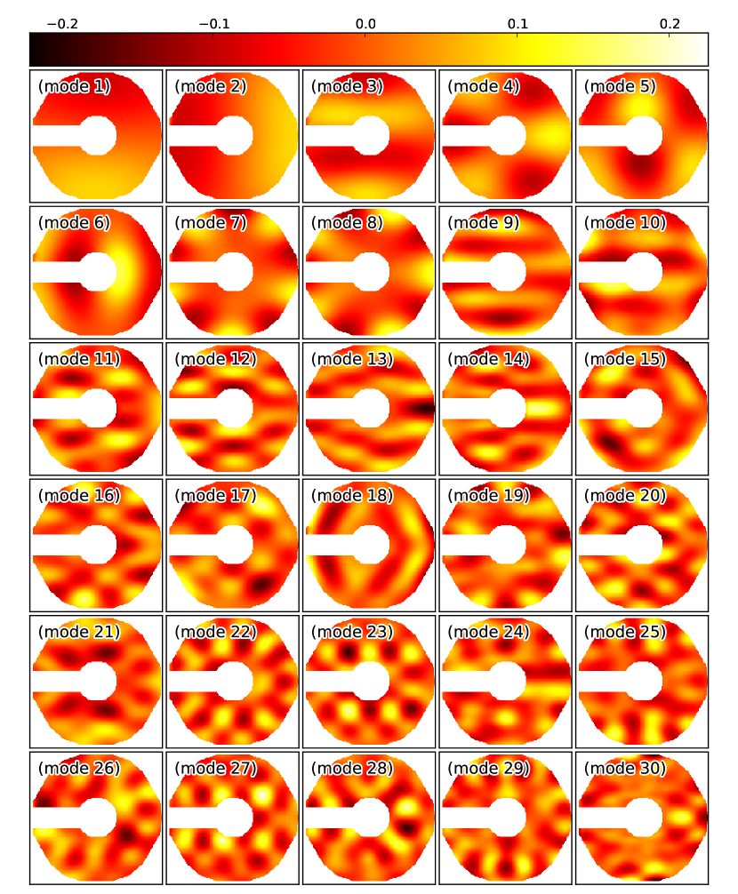
Figure 3: Representation of the first 30 SVD modes for the asymmetric pupil geometry shown in Fig. 2, sorted in order of decreasing significance (proportional to their associated singular value). All modes are represented using a common color scale, that spans the $\pm$0.2 radian range.

4.2 Optimization of the pseudo inverse for wavefront reconstruction

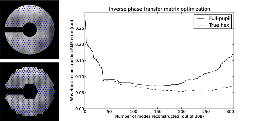
Figure 4: Curve of the APF-WFS wavefront reconstruction error (RMS) as a function of the number of modes included in the reconstruction. Two curves are shown to highlight the impact of the discrete representation of the wavefront. The solid line curve, shows the reconstruction RMS for the circular pupil shown in Fig. 2, and reproduced in the top left panel. The figure shows that including the first 40 modes exhibits the most important increase in the wavefront reconstruction fidelity, which then slowly increases until reaching an optimum around 150 modes. Including more modes however increases the reconstruction error. The dashed line curve shows how the reconstruction RMS evolves for the labeled ”true hex” pupil (bottom left panel) that more closely matches the discrete sampling used to model the optical system.

While fairly dense, the 309-element discrete representation of the pupil used to establish the linear relation for this APF-WFS remains an approximate representation of the continuous circular aperture that is the real pupil. While not significant for low-order modes of the wavefront, the impact of this discrete sampling is expected to increase for the high order modes. This, combined with the fact that the same high order modes, are associated to small singular values (for this geometry, the singular values span over three orders of magnitude from $\sim$0.1 for the lowest to $\sim$150 for the highest), suggests that the wavefront reconstruction fidelity by APF-WFS will depend on the total fraction of modes one tries to reconstruct. The result of a series of simulations, presented here, involving the reconstruction of an identical input wavefront using different reconstructions illustrates this property.

The input wavefront is a Kolmogorov phase screen, scaled down to a Strehl ratio $\sim$ 85 %. One asymmetric pupil mask, such as the one shown in Fig. 2 is used to simulate the acquisition of one single, photon noise free PSF, processed following the procedure highlighted in Sec. 3. We look at the result of a reconstruction of the input wavefront, based on the direct inversion of eq. 1:

$$\varphi=\mathbf{A_{k}^{+}}\cdot\Phi,$$ (3)

where $\mathbf{A_{k}^{+}}$ is one possible pseudo-inverse of the phase transfer matrix $\mathbf{A}$, calculated only after keeping the first $k$ singular values contained in $\mathbf{\Sigma}$:

$$\mathbf{A_{k}^{+}}=\mathbf{V}\cdot\mathbf{\Sigma_{k}^{+}}\cdot\mathbf{U^{T}}.$$ (4)

Each of these pseudo inverses then acts upon the same sampled Fourier phase vector $\Phi$ to produce an estimate of the wavefront. Fig. 4 plots the reconstruction error RMS as a function of the number of modes used for the pseudo inverse of the phase transfer matrix, using anything between one and 309 modes (the maximum for this pupil model). The solid-line curve shows the evolution of the reconstruction error for the a simulated circular aperture like shown in Fig. 2. One will observe that the error exhibits its most rapid improvement when the number of modes included in the reconstruction increases from 1 to about 40. This is somewhat expected, given that a Kolmogorov wavefront exhibits more power in the low-spatial frequencies. The reconstruction keeps slowly improving and reaches an optimum when 150 modes are used. Beyond that, the wavefront reconstruction residuals eventually increase, and the performance of the reconstruction degrades. With noise-free data, even the low-significance singular values corresponding to high spatial frequency modes should be well reconstructed, so this reduction of the wavefront reconstruction fidelity requires another explanation: the unperfect match between the hexagonal grid sampling and the actual pupil geometry, to explain this behavior. To confirm this hypothesis, Fig. 4 also shows the residuals obtained under identical conditions of wavefront and signal to noise, with a pupil mask, labeled “true hex”, that more closely matches the sampling used in the linear model: while the inclusion of the first 40 modes shows the same increase as with the circular pupil, the reconstruction fidelity keeps improving as the number of included modes increases. While an optimum is nevertheless observed (around 200 modes), the inclusion of all 309 available modes in the reconstruction does not significantly degrade the performance. The RMS can in fact be brought abitrarily close to zero by reducing the size of the sub-apertures of the “true hex” model or equivalently, by filtering out more aggressively the spatial frequency content beyond the sampling.

While a pupil mask with this “true hex” geometry can easily be manufactured, one may just as easily cknowledge this characteristic as a feature of the APF-WFS, and deliberately choose to adjust the total number of modes used in the reconstruction to the optimum found for a simulation in the noise-free case. The close loop results shown in the next section will therefore be limited to the reconstruction of the first 150 modes.

4.3 Steady state close-loop simulation

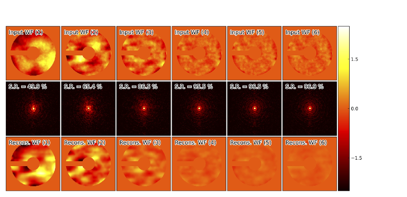
Figure 5: Sequence of wavefronts and resulting PSFs in a close-loop simulation of the APF-WFS, for 150 modes. The starting point of the simulation is a static Kolmogorov-type wavefront with a RMS 0.8 radians, resulting in a 50 % Strehl PSF. From left to right, the figure shows the impact of successive iterations of the APF-WFS. The top row shows the simulated wavefront used to produce the (photon-noise limited) PSFs shown in the middle row. The bottom row shows the wavefront reconstructed from the analysis of the PSFs by the APF-WFS. All the wavefronts are represented using a common color scale, that spans the $\pm$2 radian range.

One anticipated application of this technique is the characterization of the small non-common path error between the fast wavefront sensor arm and the science camera in an XAO system. This simulation illustrates this use case of the technique. After the initial close loop on the high order wavefront sensor, the Strehl ratio on the science focal image is of the order of 50 %, that corresponds to a wavefront RMS error of 0.8 radians.

For each iteration, a photon noise limited ($10^{5}$ photons for this series of images) single PSF is acquired, and the wavefront reconstructed by the APF-WFS is then fed back to the upstream high order wavefront sensor to offset its “flat” shape.

The simulation does not include any modeling of the deformable mirror, and simply assumes that the wavefront determined by the APF-WFS can be perfectly accounted for by the wavefront control system. Fig. 5 shows the result of five consecutive iterations of one such close-loop simulation, reconstructing the first 150 SVD modes of the wavefront each time. Three iterations are sufficient to bring the original 50 % Strehl ratio PSF to a steady Strehl level better than 95 %. Given that the linear model holds as long as $\varphi<1$ radian, the method will converge with an initial Strehl as low as $\sim 35$ %.

4.4 Sensitivity

In his overview of the limits of adaptive optics, Guyon (2005) defines a parameter noted $\beta_{p}$ that characterizes the sensitivity to photon noise of a wavefront sensor. The RMS reconstruction error by a wavefront sensor $\sigma_{m}$ for a single mode due to photon noise is equal to:

$$\sigma_{m}=\beta_{p}\sqrt{\frac{1}{n_{ph}}},$$ (5)

where $n_{ph}$ represents the total number of photons used by the sensor to reconstruct this mode. According to Guyon (2005), the ideal wavefront sensor exhibits a photon noise sensitivity criterion $\beta_{p}=1$, for each mode sensed. For reference, one of the best known and widely used wavefront sensing techniques: the Shack-Hartmann, exhibits a very non-uniform sensitivity over the modes it covers, with a peak sensitivity location that depends on the number of elements in the Hartmann screen. It is especially poorly sensitive ($\beta_{p}>>1$) for lower modes.

To illustrate how close to the ideal wavefront sensor the APF-WFS approach is, Fig. 6 plots three curves that show the evolution of the RMS wavefront reconstruction error for different level of illumination (10⁴, 10⁵ and 10⁶ photons), for a random wavefront with a Kolmogorov-type structure and a Strehl ratio of 85 %. The three curves, in this linear-log plot, equidistant in the vertical direction, show that the overall performance follows the expected $1/\sqrt{n_{ph}}$ trend (cf. eq. 5).

For each of these series of simulations, Fig. 6 also plots a dashed line, that represents the behavior of the ideal wavefront sensor described by Guyon (2005), with constant and optimal sensitivity $\beta_{p}=1$ for all modes:

$$\sigma=\sqrt{\frac{n_{m}}{n_{ph}}},$$ (6)

where $n_{m}$ and $\sigma$ now respectively represent the total number of modes included in the reconstruction, and the total RMS wavefront error in radians. The close match between the three solid lines and the dashed lines over the wide range of number of modes covered (from 10 to 100) is remarkable and demonstrates that the APF-WFS, in the high-Strehl regime where it is expected to operate, exhibits almost optimal sensitivity, making it a very attractive option, in comparison to more classical wavefront sensors.

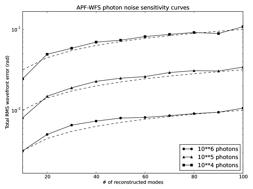
Figure 6: Sensitivity study of the APF-WFS. For three levels of total illumination (10⁴, 10⁵ and 10⁶ photons), the figure shows the evolution of the total RMS wavefront reconstruction error (in radians) due to photon noise.

5 Conclusion

This presentation of the asymmetric pupil Fourier wavefront sensor completes the theoretical study of the linear model first used to introduce the notion of kernel-phase. The linear model, although only valid in the high Strehl regime, is very powerful. The eigen vectors corresponding to zero singular values lead to kernel-phases, that in turn encode information about the target of interest, and the eigen vectors corresponding to non-zero singular values provide information about the wavefront.

To recover the wavefront, some asymmetry needs to be introduced in the pupil, and one (or more) mask such as the one used for this work is a simple addition with a minimal impact, that most XAO instruments in the making should be able to afford and accomodate. Using this mask alone and a calibration source indeed enables the characterization of the wavefront from the final science detector in an accurate and very efficient manner. The region of the pupil hidden by the asymmetric mask is obviously not accounted for, and for a complete characterization of the wavefront over the entire pupil, serial introduction of a pair of masks with asymmetric arms at different azimuths is required.

Some improvements to this approach can already be anticipated: the discrete grid model may be refined by simply (1) increasing its density, and (2) including coefficients to take into account the fact that some sample points are on the edge of the pupil. The latter point may become an essential addition if one wants to make the technique compatible with apodized pupils, which are required for high contrast coronagraphy.

Given its appealing photon noise sensitivity properties, and the relatively weak impact on the overall PSF morphology, a close loop on-sky operation appears as a viable possibility, for non-coronagraphic observations. In rich fields, well separated PSFs could simultaneously be used and the corresponding estimates of the wavefront averaged to increase the signal to noise ratio. The technique as it is, focuses on the phase: wavefront amplitude errors which would require a dedicated simultaneous image of the pupil, are going to be interpreted as phase aberrations. If such amplitude errors are significant, or if the field of the instrument extends beyond the anisoplanatic patch, the technique, looking at multiple sources may however be able to do a more complete tomographic reconstruction of the wavefront in a high Strehl MCAO system, and identify the origin of amplitude aberrations.

All simulations done so far were monochromatic, which is acceptable given that the primary application is the characterization of non-common path error in an XAO system using an internal calibration source. But an on-sky close-loop system will require operation in a broader band, and future work should explore the impact of broad band on general performance of the wavefront sensor. While one expects it to degrade somewhat, positive experience with kernel-phase analysis of data acquired in broad band filters (up to 40 %) demonstrates that the linear model still holds, suggesting that the proposed approach should remain valid.

The technique is currently being implemented on the SCExAO system, with two masks with the asymmetric arm at different position angles, so as to be able to recover the wavefront over the entire pupil. A more detailed description of this implementation along with an experimental characterization of the sensor’s performance will be the object of a future publication.

$$I=||\mathcal{F}(Ae^{i\varphi})||^{2},$$ (1)

where $A$ and $\varphi$ respectively stand for the amplitude and phase of the wavefront in the pupil, and $\mathcal{F}$ symbolizes the Fourier Transform. The so-called Fourier- or uv-plane, as it is used in the paper, is the Fourier Transform of the image, and equivalent to the autocorrelation of the complex amplitude in the pupil plane, by virtue of the convolution theorem.

$$\mathcal{A}=Ae^{i\varphi}\otimes Ae^{i\varphi}.$$ (2)

In general, Kernel-phase and the wavefront sensing idea presented in this paper rely on the assumption that wavefront errors are small, so that the expression for the complex amplitude can be linearized: $Ae^{i\varphi}\approx A(1+i\varphi)$. To simplify the notations, the functions describing the amplitude and phase in the pupil will be written as functions of a single variable $x$. Using the linearization, and eliminating second order terms, the convolution product of eq. 2 can be explicided as follows:

$$\mathcal{A}(u) \approx \int_{-\infty}^{+\infty}A(x)A(x+u)(1+i\varphi(x)+i\varphi(x+u))\,dx$$ (3)

$$= \int_{-\infty}^{+\infty}A(x)A(x+u)\,dx+i\int_{-\infty}^{+\infty}A(x)A(x+u)\varphi(x+u)\,dx+i\int_{-\infty}^{+\infty}A(x)A(x+u)\varphi(x)\,dx.$$ (4)

The first (real) term of eq. 4 only depends on the function describing the pupil amplitude $A(x)$, and not on the wavefront error $\varphi(x)$. We will therefore from now on only consider the imaginary part of this autocorrelation. To further simplify the equations, we introduce one new function $B(x)=A(x)\varphi(x)$. The imaginary part of this autocorrelation can be written as:

$$\Im(\mathcal{A}(u))=\int_{-\infty}^{+\infty}A(x)B(x+u)\,dx+\int_{-\infty}^{+\infty}A(x+u)B(x)\,dx.$$ (5)

A variable change $x^{\prime}=x+u$ for the second integral term of eq. 5 allows to rewrite the imaginary part of the autocorrelation as:

$$\Im(\mathcal{A}(u))=\int_{-\infty}^{+\infty}A(x)B(x+u)\,dx+\int_{-\infty}^{+\infty}A(x)B(x-u)\,dx.$$ (6)

The infinte integration domain can be split into two semi-infinite domains:

$$\Im(\mathcal{A}(u))=\int_{-\infty}^{0}A(x)B(x+u)\,dx+\int_{0}^{+\infty}A(x)B(x+u)\,dx+\int_{-\infty}^{0}A(x)B(x-u)\,dx+\int_{0}^{+\infty}A(x)B(x-u)\,dx,$$ (7)

and one additional variable change $x^{\prime}=-x$ is used for the integral terms over the negative domains. Eq. 7 can be rewritten as:

$$\Im(\mathcal{A}(u))=-\int_{0}^{+\infty}A(-x)B(-x+u)\,dx+\int_{0}^{+\infty}A(x)B(x+u)\,dx-\int_{0}^{+\infty}A(-x)B(-x-u)\,dx+\int_{0}^{+\infty}A(x)B(x-u)\,dx.$$ (8)

The pupil is assumed to be symmetric, so that the amplitude function verifies $A(-x)=A(x)$. Similarly, the even component of the pupil phase also verifies $\varphi(-x)=\varphi(x)$. For eq. 8, this translates into $B(-x)=B(x)$. For an even mode, the imaginary part of the autocorrelation becomes:

$$\Im(\mathcal{A}(u))=-\int_{0}^{+\infty}A(x)B(x-u)\,dx+\int_{0}^{+\infty}A(x)B(x+u)\,dx-\int_{0}^{+\infty}A(x)B(x+u)\,dx+\int_{0}^{+\infty}A(x)B(x-u)\,dx.$$ (9)

The reader will observe that all terms in eq. 9 cancel out, which demonstrates that even modes of the pupil wavefront cannot be sensed in the Fourier plane. By contrast, the antisymmetric properties of an odd mode translates into $B(-x)=-B(x)$. Two of the four terms cancel out, leading to the simplified expression for the imaginary part of the autocorrelation:

$$\Im(\mathcal{A}(u))=2\int_{0}^{+\infty}A(x)B(x+u)\,dx.$$ (10)

References

- Bouchez et al. (2010) Bouchez, A. H., Dekany, R. G., Roberts, J. E., et al. 2010, in Society of Photo-Optical Instrumentation Engineers (SPIE) Conference Series, Vol. 7736, Society of Photo-Optical Instrumentation Engineers (SPIE) Conference Series
- Guyon (2005) Guyon, O. 2005, ApJ, 629, 592
- Koechlin et al. (1996) Koechlin, L., Lawson, P. R., Mourard, D., et al. 1996, Appl. Opt., 35, 3002
- Kraus et al. (2008) Kraus, A. L., Ireland, M. J., Martinache, F., & Lloyd, J. P. 2008, ApJ, 679, 762
- Marois et al. (2003) Marois, C., Doyon, R., Nadeau, D., Racine, R., & Walker, G. A. H. 2003, in EAS Publications Series, Vol. 8, EAS Publications Series, ed. C. Aime & R. Soummer, 233–243
- Marois et al. (2006) Marois, C., Lafrenière, D., Doyon, R., Macintosh, B., & Nadeau, D. 2006, ApJ, 641, 556
- Marois et al. (2008) Marois, C., Macintosh, B., Barman, T., et al. 2008, Science, 322, 1348
- Martinache (2004) Martinache, F. 2004, Journal of Optics A: Pure and Applied Optics, 6, 216
- Martinache (2010) Martinache, F. 2010, ApJ, 724, 464
- Martinache (2011) Martinache, F. 2011, in Society of Photo-Optical Instrumentation Engineers (SPIE) Conference Series, Vol. 8151, Society of Photo-Optical Instrumentation Engineers (SPIE) Conference Series
- Martinache (2012) Martinache, F. 2012, in Society of Photo-Optical Instrumentation Engineers (SPIE) Conference Series, Vol. 8445, Society of Photo-Optical Instrumentation Engineers (SPIE) Conference Series
- Martinache et al. (2012) Martinache, F., Guyon, O., Clergeon, C., & Blain, C. 2012, ArXiv e-prints
- Martinache et al. (2011) Martinache, F., Guyon, O., Garrel, V., et al. 2011, in Society of Photo-Optical Instrumentation Engineers (SPIE) Conference Series, Vol. 8151, Society of Photo-Optical Instrumentation Engineers (SPIE) Conference Series
- Michelson & Pease (1921) Michelson, A. A. & Pease, F. G. 1921, ApJ, 53, 249
- Peters et al. (2012) Peters, M. A., Groff, T., Kasdin, N. J., et al. 2012, ArXiv e-prints
- Pope et al. (2012) Pope, B., Martinache, F., & Tuthill, P. G. 2013, ArXiv e-prints
- Sauvage et al. (2010) Sauvage, J.-F., Fusco, T., Petit, C., et al. 2010, in Society of Photo-Optical Instrumentation Engineers (SPIE) Conference Series, Vol. 7736, Society of Photo-Optical Instrumentation Engineers (SPIE) Conference Series
- Wallace et al. (2010) Wallace, J. K., Burruss, R. S., Bartos, R. D., et al. 2010, in Society of Photo-Optical Instrumentation Engineers (SPIE) Conference Series, Vol. 7736, Society of Photo-Optical Instrumentation Engineers (SPIE) Conference Series
- Zhai et al. (2012) Zhai, C., Vasisht, G., Shao, M., et al. 2012, in Society of Photo-Optical Instrumentation Engineers (SPIE) Conference Series, Vol. 8447, Society of Photo-Optical Instrumentation Engineers (SPIE) Conference Series