Semiclassical approximation solved by Monte Carlo as an efficient impurity solver for dynamical mean field theory and its cluster extensions

Abstract

We propose that a combination of the semiclassical approximation with Monte Carlo simulations can be an efficient and reliable impurity solver for dynamical mean field theory equations and their cluster extensions with large cluster sizes. In order to show the reliability of the method, we consider two test cases: (i) the single-band Hubbard model within the dynamical cluster approximation with 4- and 8-site clusters and (ii) the anisotropic two-orbital Hubbard model with orbitals of different band width within the single-site dynamical mean field theory. We compare the critical interaction $U_{c}/t$ with those obtained from solving the dynamical mean field equations with continuous time and Hirsch-Fye quantum Monte Carlo. In both test cases we observe reasonable values of the metal-insulator critical interaction strength $U_{c}/t$ and the nature of Mott physics in the self-energy behavior. While some details of the spectral functions cannot be captured by the semiclassical approximation due to the freezing of dynamical fluctuations, the main features are reproduced by the approach.

I Introduction

The single-site dynamical mean field theory (DMFT) approach has been extensively employed to explore the properties of the Hubbard model and, in general, of strongly correlated materials Georges1996 ; Kotliar2004 ; Kotliar2006 . Though the metal-Mott insulator transition can be successfully accounted for within the DMFT approximation where dynamical fluctuations alone are emphasized, interesting physical phenomena such as spin density waves and superconductivity can not be properly described due to the absence of spatial fluctuations. Cluster-extensions of DMFT like cellular-dynamical mean field theory (CDMFT) Kotliar2006 and dynamical cluster approximation (DCA) Hettler1998 ; Maier2005 can take into account the inter-site spatial fluctuations within the size of the cluster in addition to the dynamical fluctuations. For example, cluster extensions of DMFT with 4-site clusters in combination with continuous time quantum Monte Carlo (CT-QMC) or exact diagonalization (ED) can partly capture the physics of Fermi liquid (FL), non-FL (or pseudo gap), Mott insulator, and superconductivity on an equal footing Civelli2005 ; Zhang2007 ; Sakai2009 ; Liebsch2009 ; Sentef2011 ; Sordi2012 ; Tocchio2012 . However, due to the computational expense of CT-QMC and ED, the system size is still limited to only small clusters and not all physical properties can be equally precisely studied. In particular, the hybridization expansion CT-QMC approach is able to treat small cluster sizes up to only $N_{c}=4$ due to an exponential increase of the local Hilbert space with $N_{c}$ Werner2006(1) ; Werner2006(2) . The ED approach encounters a similar problem. Even though other impurity solvers like the interaction expansion CT-QMC approach are applicable to large cluster systems, the computational expense is proportional to the square of three quantities: the interaction strength $U$, the inverse of the temperature $T$, and the number of cluster sites $N_{c}$ Rubtsov2005 ; Gull2011 . The Hirsch-Fye QMC (HF-QMC) Hirsch1985 ; Hirsch1986 impurity solver shows a computational expense proportional to $N_{c}^{3}L^{3}$ where $L$ is the number of slices in the imaginary time (temperature). More recently, Khatami et al. Khatami2010 proposed the determinantal QMC (DQMC) Blankenbecler1981 as a new impurity solver where the computational expense has a $(N_{c}+N_{c}N_{a})^{3}L$ dependence with $N_{a}$ being the number of bath sites connected to each cluster site. This is though a Hamiltonian-based impurity solver that requires an explicit form of a cluster Anderson impurity model to calculate the self-energy. In contrast, CT-QMC, Hirsch-Fye QMC and the method under discussion in the present work, the semiclassical approximation (SCA), are action-based impurity solvers. Summarizing and in view of the above, a fast and reliable impurity solver for DMFT calculations and its cluster extensions with large cluster sizes is still highly desirable.

The SCA has been proposed as an impurity solver for DMFT and its cluster extensions Okamoto2005 ; Fuhrmann2007 ; Lee2008 . (i) This impurity solver is fast since the computational expense depends only on calculation time at each Matsubara frequency of the inverse of a matrix with dimensions $N_{c}\times N_{c}$ (for a cluster with $N_{c}$ sites) or $L_{c}\times L_{c}$ (for a single site with $L_{c}$ orbitals), where $L_{c}$ is the number of orbitals. (ii) While it cannot properly account for Fermi-liquid behavior in the weak-coupling limit Okamoto2005 , and in general, it is not adequate at low temperatures due to the freezing of quantum fluctuations in the method, it is especially suited for large interaction strength and multi-sites where for example the powerful interaction expansion CT-QMC method is very costly. (iii) It provides self-energy information directly on the real frequency axis. This avoids the uncertainty from analytic continuation which has to be done in various QMC approaches Wang2009 . The previously used SCA approach Okamoto2005 ; Fuhrmann2007 ; Lee2008 was limited though to consider small cluster sizes of $N_{c}=4$ due to the difficulty of the multi-dimensional integrations.

In the present work, we propose to combine the SCA approach with the Monte Carlo (MC) method. The latter is used to evaluate the multi-dimensional integrals. We apply our scheme to two test cases: (i) the one-orbital Hubbard model on the square lattice at half-filling within the DCA with cluster sizes $N_{c}=4$ and $N_{c}=8$ and (ii) the anisotropic two-orbital Hubbard model with different band widths on the Bethe lattice at half-filling within single-site DMFT. We present the density of states, momentum dependent spectral functions, and momentum dependent self-energy as a function of real frequency $\omega$. For case (i) we find that even though the Fermi liquid behavior is not obtained comment1 , the critical onsite Coulomb interaction $U_{c}/t$ for the metal-insulator transition calculated by our SCA approach for both cluster sizes shows a reasonable agreement with the value obtained from CT-QMC which should be numerically exact. In particular, we find that the behavior of the density of states at the Fermi level in each momentum sector obtained from both SCA and CT-QMC approaches are quantitatively consistent with each other. For case (ii) we also find a reasonable agreement of $U_{c}/t$ obtained from SCA and HF-QMC. The orbital-selective phase transition is also correctly detected. However, we observe that if the band-width difference between narrow and wide orbitals is large, a causality problem appears in the SCA results.

The paper is organized as follows. In Sec. II we present the general formalism of the semiclassical approximation and its application to cases (i) and (ii). In Sec. III, we discuss our SCA calculations and compare some results with both CT-QMC and HF-QMC and finally, in Sec. IV we summarize our findings.

II SEMICLASSICAL APPROXIMATION

In this section we will review the formalism of the SCA approach Okamoto2005 ; Fuhrmann2007 ; Lee2008 adapted to the two test cases considered in this work; the 8-site DCA and two-orbital DMFT systems with paramagnetic solutions.

II.1 General formalism

The partition function can be written as:

$$Z=\int D\left[c^{\dagger}c\right]e^{-(S_{0}+S_{\rm int})},$$ (1)

where

$$S_{\rm int}=U\int_{0}^{\beta}d\tau\sum_{i}n_{i\uparrow}(\tau)n_{i\downarrow}(\tau)$$ (2)

and

$$S_{0}=-\int_{0}^{\beta}d\tau\int_{0}^{\beta}d\tau^{\prime}\psi_{\sigma}^{\dagger}(\tau)\hat{a}_{\sigma}(\tau,\tau^{\prime})\psi_{\sigma}(\tau^{\prime}),$$ (3)

where $\psi_{\sigma}^{\dagger}=(c_{1\sigma}^{\dagger}\ldots c_{l\sigma}^{\dagger})$ and $c_{i\sigma}^{\dagger}$ ($c_{i\sigma}$) is a Grassmann number corresponding to the Fermionic creation (annihilation) operator at site $i$ and spin $\sigma$, and $\hat{a}_{\sigma}=\sum_{\xi}a_{\xi\sigma}\hat{K}_{\xi\sigma}$ where $a_{\xi\sigma}$ are inverted frequency- dependent Weiss fields and $\hat{K}_{\xi\sigma}$ are $l\times l$ matrices defined according to the chosen cluster. Here, $l$ denotes the number of sites in the multi-site system (case (i)) or two times the number of orbitals in the multi-orbital system (case(ii)), and $\xi$ denotes the distance between two sites within the cluster. For example, $a^{-1}_{0\sigma}$ means the local (on-site) Weiss field while $a^{-1}_{\xi\sigma}$ is the inter-site Weiss field with the sites located at a distance $\xi$-th apart. The orthogonality is imposed by

$${\rm Tr}\left[\hat{K}_{\xi\sigma}\hat{K}_{\xi^{\prime}\sigma^{\prime}}\right]=l\delta_{\xi\xi^{\prime}}\delta_{\sigma\sigma^{\prime}}.$$ (4)

$n_{i\uparrow}(\tau)n_{i\downarrow}(\tau)$ in the decoupling scheme can be written as:

$$n_{i\uparrow}(\tau)n_{i\downarrow}(\tau)=\frac{1}{4}(N_{i}(\tau)^{2}-M_{i}(\tau)^{2}),$$ (5)

where $N_{i}=(n_{i\uparrow}+n_{i\downarrow})$ and $M_{i}=(n_{i\uparrow}-n_{i\downarrow})$ are the particle number and magnetization, respectively. In terms of these definitions and within the SCA approximation, the partition function transforms into

$$Z=\int D\left[c^{\dagger}c\right]e^{\int_{0}^{\beta}d\tau\int_{0}^{\beta}d\tau^{\prime}\psi_{\sigma}^{\dagger}(\tau)\hat{a}_{\sigma}(\tau,\tau^{\prime})\psi_{\sigma}(\tau^{\prime})+\frac{U}{4}\int_{0}^{\beta}\sum_{i}M_{i}^{2}(\tau)}.$$ (6)

where the $N_{i}^{2}(\tau)$ term, which describes charge fluctuations, is neglected in the SCA approximation. This expression can be rewritten as

$$Z=\int D\left[c^{\dagger}c\right]\int_{-\infty}^{\infty}\prod_{i=1}^{k}d\phi_{i}e^{S},$$ (7)

with

$$S=\int_{0}^{\beta}d\tau\bigg{(}\int_{0}^{\beta}d\tau^{\prime}\psi_{\sigma}^{\dagger}(\tau)\hat{a}_{\sigma}(\tau,\tau^{\prime})\psi_{\sigma}(\tau^{\prime})-\Big{(}\frac{\phi_{i}^{2}}{4U}-\frac{\phi_{i}M_{i}(\tau)}{2}\Big{)}\bigg{)}.$$ (8)

Here we assume that the new auxiliary fields $\phi_{i}(\tau)$, which are given by a continuous Hubbard-Stratonovich transformation, are $\tau$-independent $(\phi_{i}(\tau)\equiv\phi_{i})$.

We replace $M_{i}(\tau)$ by

$$M_{i}(\tau)=\int_{0}^{\beta}d\tau^{\prime}\sum_{ss^{\prime}}c_{is}^{\dagger}(\tau)\sigma^{z}\delta(\tau-\tau^{\prime})c_{is^{\prime}}(\tau^{\prime}),$$ (9)

where $\sigma^{z}$ is the third Pauli matrix. Via a Grassmann integration and Fourier transformation, the partition function (Eq. (6)) is finally given as

$$Z=\int_{-\infty}^{\infty}\prod_{i=1}^{k}d\phi_{i}e^{\displaystyle-\frac{\beta\phi_{i}^{2}}{4U}+\sum_{\omega_{n}}{\rm ln}{\rm Det}\left[-\beta(\hat{a}_{\sigma}(i\omega_{n})+\frac{1}{2}\phi_{i}\sigma_{z})\right]},$$ (10)

where $\omega_{n}$ are Fermionic Matsubara frequencies and $k$ is the dimension of integrations. The impurity Green’s function can be obtained as $\hat{G}^{\rm imp}_{\sigma}(i\omega_{n})=\sum_{\xi}G_{\xi\sigma}(i\omega_{n})\hat{K}_{\xi\sigma}$ where $G_{\xi\sigma}(i\omega_{n})$ is

$$G_{\xi\sigma}(i\omega_{n})=\frac{1}{l}\frac{\partial{\rm ln}Z}{\partial a_{\xi\sigma}(i\omega_{n})}$$ (11)

where $l$ is the normalization factor which is given by Eq. (4). The Green’s function on the real frequency $\omega$ is also calculated by Eq. (11) with replacement of $\omega_{n}$ into $\omega+i\delta$. In our calculations we consider a broadening factor $\delta=0.003$. The integration in $i=N_{c}\times m\times(2m-1)$ dimensions for classical fields $\phi_{i}$ is evaluated by the MC approach, where $N_{c}$ is the number of cluster sites, $m$ is the number of orbitals, and the weight function $W(\phi_{i})$ for the MC simulations is given as

$${\rm ln}W(\phi_{i})=-\frac{\beta\phi_{i}^{2}}{4U}+\sum_{\omega_{n}}\rm{ln}\rm{Det}\left[-\beta(\hat{a}_{\sigma}(i\omega_{n})+\frac{1}{2}\phi_{i}\sigma_{z})\right].$$ (12)

II.2 8-site dynamical cluster approximation

The partition function in the SCA approach is described in a real-space basis in Eqs. (1)-(3). The $8\times 8$ matrices of inversed Weiss fields (Eq. (10) and Eq. (11)) in the 8-site DCA calculations for the Hubbard model on the square lattice are given as

$$\hat{a}(i\omega_{n})=\left(\begin{array}[]{cccccccc}a_{0}&\frac{a_{2}}{\sqrt{2}}&\frac{a_{1}}{2}&\frac{a_{1}}{2}&\frac{a_{2}}{\sqrt{2}}&a_{3}&\frac{a_{1}}{2}&\frac{a_{1}}{2}\\ \frac{a_{2}}{\sqrt{2}}&a_{0}&\frac{a_{1}}{2}&\frac{a_{1}}{2}&a_{3}&\frac{a_{2}}{\sqrt{2}}&\frac{a_{1}}{2}&\frac{a_{1}}{2}\\ \frac{a_{1}}{2}&\frac{a_{1}}{2}&a_{0}&\frac{a_{2}}{\sqrt{2}}&\frac{a_{1}}{2}&\frac{a_{1}}{2}&a_{3}&\frac{a_{2}}{\sqrt{2}}\\ \frac{a_{1}}{2}&\frac{a_{1}}{2}&\frac{a_{2}}{\sqrt{2}}&a_{0}&\frac{a_{1}}{2}&\frac{a_{1}}{2}&\frac{a_{2}}{\sqrt{2}}&a_{3}\\ \frac{a_{2}}{\sqrt{2}}&a_{3}&\frac{a_{1}}{2}&\frac{a_{1}}{2}&a_{0}&\frac{a_{2}}{\sqrt{2}}&\frac{a_{1}}{2}&\frac{a_{1}}{2}\\ a_{3}&\frac{a_{2}}{\sqrt{2}}&\frac{a_{1}}{2}&\frac{a_{1}}{2}&\frac{a_{2}}{\sqrt{2}}&a_{0}&\frac{a_{1}}{2}&\frac{a_{1}}{2}\\ \frac{a_{1}}{2}&\frac{a_{1}}{2}&a_{3}&\frac{a_{2}}{\sqrt{2}}&\frac{a_{1}}{2}&\frac{a_{1}}{2}&a_{0}&\frac{a_{2}}{\sqrt{2}}\\ \frac{a_{1}}{2}&\frac{a_{1}}{2}&\frac{a_{2}}{\sqrt{2}}&a_{3}&\frac{a_{1}}{2}&\frac{a_{1}}{2}&\frac{a_{2}}{\sqrt{2}}&a_{0}\\ \end{array}\right),$$ (13)

where spin indices are omitted for simplicity and the normalization factors $\frac{1}{2}$ and $\frac{1}{\sqrt{2}}$ are introduced in order to fulfill the orthogonality condition Eq. ((4)). The indices $\xi=0,1,2$, and $3$ indicate on-site, 1st neighbor, 2nd neighbor, and 3rd neighbor, respectively. The cluster we used for constructing the $\hat{a}(i\omega_{n})$ matrices with periodic boundary condition is shown in Fig. 1 (a) and the division of BZ for DCA calculations is presented in Fig. 1 (b). The real-space impurity Green’s functions in Eq. ((11)) are more clearly expressed as

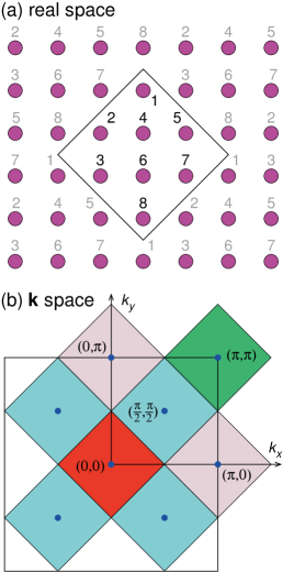
Figure 1: (Color online) Cartoons for (a) the eight-site dynamical cluster approximation in real space and for (b) the division of the Brillouin zone in momentum space we used.

$$G_{\xi}(i\omega_{n})=\frac{1}{l}\frac{1}{\rm{Det}\left[\hat{A}(a_{\xi}(i\omega_{n}))\right]}\frac{\partial}{\partial a_{\xi}(i\omega_{n})}\rm{Det}\left[\hat{A}(a_{\xi}(i\omega_{n}))\right],$$ (14)

where $\hat{A}(a_{\xi}(i\omega_{n}))=-\beta(\hat{a}(i\omega_{n})+\phi_{i})$ are $8\times 8$ matrices with spin index $\sigma$. The impurity Green’s function in Eq. (14) is measured by

$$\frac{1}{\rm{Det}\left[\hat{A}(a_{\xi})\right]}\frac{\partial}{\partial a_{\xi}}\rm{Det}\left[\hat{A}(a_{\xi})\right]=\rm{tr}\left[\hat{A}^{-1}(a_{\xi})\frac{\partial\hat{A}(a_{\xi})}{\partial a_{\xi}}\right].$$ (15)

II.3 2-orbital dynamical mean field theory

The interaction term of the Hamiltonian for the 2-orbital system (test case (ii)) is given as

$$H_{\rm int}=U\sum_{i\eta}n_{i\eta\uparrow}n_{i\eta\downarrow}+\sum_{i\sigma\sigma^{\prime}}(U^{\prime}-\delta_{\sigma\sigma^{\prime}}J_{z})n_{i1\sigma}n_{i2\sigma^{\prime}},$$ (16)

where $\eta\in\{1,2\}$ denote orbital indexes. $U$ and $U^{\prime}$ are, respectively, onsite intra-orbital and inter-orbital Coulomb interaction parameters and $J_{z}$ is the Ising Hund’s coupling term. We are not considering the spin-flip and pair hopping terms in our calculations. The inversed Weiss field is given as

$$\hat{a}(i\omega_{n})=\left(\begin{array}[]{cccc}a_{1,\uparrow}&0&0&0\\ 0&a_{1,\downarrow}&0&0\\ 0&0&a_{2,\uparrow}&0\\ 0&0&0&a_{2,\downarrow}\\ \end{array}\right).$$ (17)

We now decouple the interaction term Eq. (16) using Eq. (5):

$$n_{1\uparrow}n_{1\downarrow}=\frac{1}{4}(N_{1}^{2}-M_{1}^{2}),n_{2\uparrow}n_{2\downarrow}=\frac{1}{4}(N_{2}^{2}-M_{2}^{2}),$$

$$n_{1\uparrow}n_{2\downarrow}=\frac{1}{4}(N_{3}^{2}-M_{3}^{2}),n_{1\downarrow}n_{2\uparrow}=\frac{1}{4}(N_{4}^{2}-M_{4}^{2}),$$

$$n_{1\uparrow}n_{2\uparrow}=\frac{1}{4}(N_{5}^{2}-M_{5}^{2}),n_{1\downarrow}n_{2\downarrow}=\frac{1}{4}(N_{6}^{2}-M_{6}^{2}).$$

Neglecting charge fluctuations $N_{\xi}^{2}$, the partition function can be written as

$$\frac{Z}{Z_{0}}=e^{\displaystyle\int_{0}^{\beta}(\frac{U}{4}(M_{1}^{2}+M_{2}^{2})+\frac{U^{\prime}}{4}(M_{3}^{2}+M_{4}^{2})+\frac{U^{\prime\prime}}{4}(M_{5}^{2}+M_{6}^{2}))},$$ (18)

where $U^{\prime\prime}=U^{\prime}-J_{z}$ and

$$Z_{0}=\int D\left[c^{\dagger}c\right]e^{\displaystyle\int_{0}^{\beta}d\tau\int_{0}^{\beta}d\tau^{\prime}\psi^{\dagger}(\tau)\hat{a}(\tau,\tau^{\prime})\psi(\tau^{\prime})},$$ (19)

where $\psi^{\dagger}=(c^{\dagger}_{1\uparrow},c^{\dagger}_{1\downarrow},c^{\dagger}_{2\uparrow},c^{\dagger}_{2\downarrow})$ (compare with Eq. (3)). In order to make integration feasible, Eq. (18) is transformed into $Z=Z_{0}e^{-S}$ with

$$\begin{split}S=&-\frac{\phi_{1}^{2}+\phi_{2}^{2}}{4U}-\frac{\phi_{3}^{2}+\phi_{4}^{2}}{4U^{\prime}}-\frac{\phi_{5}^{2}+\phi_{6}^{2}}{4U^{\prime\prime}}\\ &+\int_{0}^{\beta}d\tau\frac{1}{2}\sum_{\xi=1}^{6}\phi_{\xi}M_{\xi}(\tau)\end{split}$$ (20)

where we used the continuous Hubbard-Stratonovich transformation as in Eq. (8). Next (see Eq. (9)), $M_{\xi}(\tau)$ is replaced by

$$M_{\xi}(\tau)=\int_{0}^{\beta}d\tau^{\prime}\psi^{\dagger}(\tau)\sigma_{\xi}^{z}\delta(\tau-\tau^{\prime})\psi(\tau^{\prime}).$$ (21)

Site indices are omitted due to the single-site DMFT calculation and $\sigma_{\xi}^{z}$ are $4\times 4$ matrices:

$$\sigma_{1}^{z}=\left(\begin{array}[]{cccc}1&0&0&0\\ 0&-1&0&0\\ 0&0&0&0\\ 0&0&0&0\\ \end{array}\right),\sigma_{2}^{z}=\left(\begin{array}[]{cccc}0&0&0&0\\ 0&0&0&0\\ 0&0&1&0\\ 0&0&0&-1\\ \end{array}\right)$$ (30)

$$\sigma_{3}^{z}=\left(\begin{array}[]{cccc}0&0&0&1\\ 0&0&0&0\\ 0&0&0&0\\ -1&0&0&0\\ \end{array}\right),\sigma_{4}^{z}=\left(\begin{array}[]{cccc}0&0&0&0\\ 0&0&1&0\\ 0&-1&0&0\\ 0&0&0&0\\ \end{array}\right)$$ (39)

$$\sigma_{5}^{z}=\left(\begin{array}[]{cccc}0&0&1&0\\ 0&0&0&0\\ -1&0&0&0\\ 0&0&0&0\\ \end{array}\right),\sigma_{6}^{z}=\left(\begin{array}[]{cccc}0&0&0&0\\ 0&0&0&1\\ 0&0&0&0\\ 0&-1&0&0\\ \end{array}\right)$$ (48)

Finally, the partition function is rewritten as

$$Z=\int_{-\infty}^{\infty}\prod_{\xi=1}^{6}d\phi_{\xi}e^{-V(\phi_{\xi})+\sum_{\omega_{n}}\rm{ln}\rm{Det}\left[-\beta(\hat{a}(i\omega_{n})+\frac{1}{2}\phi_{\xi}\sigma_{\xi}^{z})\right]},$$ (49)

where $V(\phi_{\xi})=\beta(\frac{\phi_{1}^{2}+\phi_{2}^{2}}{4U}+\frac{\phi_{3}^{2}+\phi_{4}^{2}}{4U^{\prime}}+\frac{\phi_{5}^{2}+\phi_{6}^{2}}{4U^{\prime\prime}})$. The impurity Green’s functions are calculated by Eq. (11).

II.4 Monte Carlo measurement

The weight functions for MC calculations have been given in Eq. (12). We employ about 400 Matsubara frequencies for performing the frequency sum in Eq. (12). The number of classical fields $\phi_{i}$ is the same as the number of cluster sites in the DCA calculations (case (i)). For case (ii) the number of classical fields is given by $(2m-1)\times m$, where $m$ is the number of orbitals. In order to avoid a local minimum problem in the MC calculation, we use around forty initial configurations and we perform about $4\times 10^{5}$ MC samplings for each different initial configuration. The computational cost for $4\times 10^{5}$ MC samplings in the 8-site DCA system is around 90 minutes on a single 4 GHz CPU machine and the error is smaller than $5\times 10^{-4}$.

III RESULTS

III.1 The metal-insulator transition in the 8-site dynamical cluster approximation

In what follows, we will show the reliability of our SCA impurity solver by presenting the results obtained for 4- and 8-site DCA calculations for a two-dimensional Hubbard model on the square lattice at half-filling (case (i)).

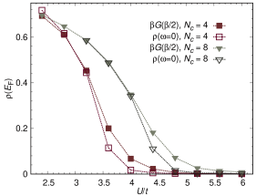
Figure 2: (Color online) The density of states at the Fermi level $\rho(\omega=0)\approx\beta G(\frac{\beta}{2})$ and $\rho(\omega=0)$, directly measured in real-frequency space within DCA(SCA), as a function of $U/t$ for $N_{c}=4$ and 8 at $T/t=1/12$. From $\rho(\omega=0)$ we find the critical metal-insulator interactions $U_{c}/t=4.4\pm 0.2$ and $5.0\pm 0.2$ for $N_{c}=4$ and 8, respectively. The error bars are smaller than symbol sizes. The deviations of between $\beta G(\frac{\beta}{2})$ and $\rho(\omega=0)$ are around ten percent. See the main text for discussion.

First, we compare the critical $U_{c}/t$ obtained from DCA(SCA) calculations with that obtained from DCA(CT-QMC) with $N_{c}=4$ and $8$. Within DCA(CT-QMC) Gull2008 ; Gull2009 $U_{c}/t=4.5$ ($N_{c}=4$) and $U_{c}/t=6.5$ ($N_{c}=8$). We would like to note that for the two-dimensional Hubbard model on the square lattice at half-filling, previous DCA calculations showed that, at finite temperature, the larger the cluster size is, the smaller the critical value of interaction $U_{c}/t$. This is due to the fact that DCA calculations account for spatial correlations only within the cluster Moukouri2001 ; Kyung2003 . This suggests that we should expect a smaller $U_{c}/t$ for increasing cluster sizes. However, this is not what it is observed above. We think that the reason for this discrepancy lies on the fact that plaquette singlet ordered states become more favorable for $N_{c}=4$ than for $N_{c}=8$ and artificially stabilize an insulating state in $N_{c}=4$. We now check whether this behavior is also observed in the SCA approach. In Fig. 2 we plot the DCA(SCA) density of states at the Fermi level obtained as (1) $\rho(\omega=0)\approx\beta G(\frac{\beta}{2})$ comment and (2) directly calculated in real-frequency space $\rho(\omega=0)$, as a function of $U/t$ for $N_{c}=4$ and $8$ at $T/t=1/12$. The imaginary time Green’s function $G(\tau)$ is calculated by the Fourier transformation of $G(i\omega_{n})$ in Eq. (11). We find $U_{c}/t=4.4\pm 0.2$ and $5.0\pm 0.2$ for $N_{c}=4$ and $8$ respectively. The trend, i.e., smaller critical interaction $U_{c}/t$ for $N_{c}=4$ than for $N_{c}=8$, is the same as in DCA(CT-QMC). We also detect that the critical interactions $U_{c}/t$ in the SCA method are slightly smaller than those calculated by the CT-QMC method. The reason why the insulating state is overestimated, is due to the fact that the auxiliary field is assumed to be $\tau$ independent in SCA, indicating a freezing of dynamical fluctuations in SCA.

Usually one always employs the relation $\rho(\omega=0)\approx\beta G(\frac{\beta}{2})$ to determine the critical interaction $U_{c}/t$ for the metal-insulator transition in DCA(CT-QMC) Gull2008 ; Gull2009 . This is done in order to avoid the performance of an analytical continuation, which will introduce some uncertainties. Therefore, it is interesting to check whether this relation is valid in all cases. Since DCA(SCA) provides results directly in real-frequency space, both definitions can be tested on the same footing. Fig.  2 shows that both definitions are in good agreement in the weak-coupling and strong-coupling regions, but they show deviations of about ten percent close to the critical value due to finite temperature effects comment . In addition, we find a causality problem in the weak-coupling region (for $U/t$ values smaller than $3.0$).

In order to test the reliability of the SCA approximation we present in Fig. 3 a quantitative comparison of $\beta G(\beta/2)$ as a function of frequency obtained by the SCA impurity solver and by CT-QMC Gull2008 for $N_{c}=4$ and inverse temperatures $\beta=3/t,6/t$. We observe a good agreement between both sets of results at high temperature regions.

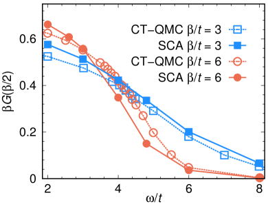
Figure 3: (Color online) Comparison of $\beta G(\frac{\beta}{2})$ in DCA(SCA) and DCA(CT-QMC) for $\beta=3.0/t$ and $6.0/t$ as a function of $\omega/t$ for $N_{c}=4$. The CT-QMC results were obtained from Ref. Gull2008, .

Next, we would like to analyze the spectral functions in different DCA cluster momentum sectors, i.e., $A({\bf K},\omega)$ at ${\bf K}=(0,0)$, $(0,\pi)$, $(\frac{\pi}{2},\frac{\pi}{2})$ and $(\pi,\pi)$ shown in Fig. 1 (b) for several values of $U/t$ at $T/t=1/12$. In Fig. 4 (a) we display the non-interacting case ($U/t=0.0$). While the weights of the spectral functions $A({\bf K},\omega)$ at ${\bf K}=(0,0)$ and $(\pi,\pi)$ sectors are well separated from each other, resembling the behavior of band insulators, the spectral functions at ${\bf K}=(0,\pi)$ and $(\frac{\pi}{2},\frac{\pi}{2})$ sectors cross the Fermi level, showing metallic behavior. The van-Hove singularity is present in the spectral function in the ${\bf K}=(\pi,0)/(0,\pi)$ sector. The behavior of $A({\bf K},\omega)$ for $N_{c}=8$ is comparable to $N_{c}=4$ results Haule2007 and can be understood in terms of the non-interacting band structure.

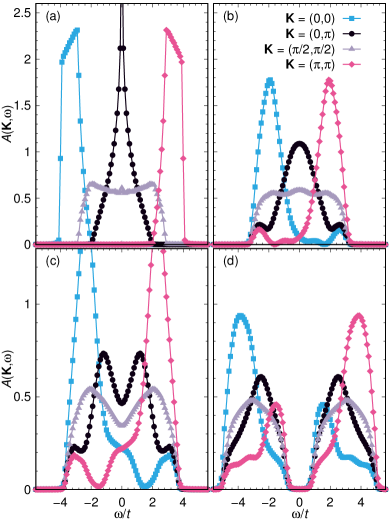
Figure 4: (Color online) The spectral functions $A({\bf K},\omega)$ in the different DCA momentum sectors ${\bf K}$ for (a) $U/t=0.0$, (b) 3.2 (c) 4.0 and (d) 6.0 at $T/t=1/12$.

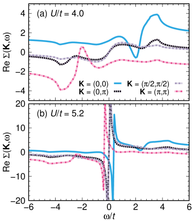
Figure 5: (Color online) The real part of self-energy ${\rm Re}(\Sigma({\bf K},\omega))$ as a function of real frequency $\omega/t$ for (a) $U/t=4.0$ and (b) $U/t=5.2$ at $T/t=1/12$.

In Fig. 4 (b) we show $A({\bf K},\omega)$ for $U/t=3.2$ (weak-coupling region). $A({\bf K},\omega)$ at ${\bf K}=(0,0)$ and $(\pi,\pi)$ intersect with each other due to the band splitting and spectral weight transfer induced by $U$. This is an indication of Mott physics. The insulating behavior still remains in these two sectors and the whole band width is slightly narrowed due to correlation effects. The van-Hove singularity that was present in the ${\bf K}=(\pi,0)$ sector in the non-interacting case, is dramatically suppressed with increasing $U/t$. The absence of a strong quasi-particle peak in the weak interaction region is due to the freezing of dynamical fluctuations. This is a shortcoming of the SCA method. As the interaction $U/t$ is increased, a pseudo-gap behavior is present with suppression of the spectral functions at ${\bf K}=(0,\pi)$ and $(\frac{\pi}{2},\frac{\pi}{2})$ at $U/t=4.0$ (Fig. 4 (c)), and the Mott insulator appears in the strong-coupling region at $U/t=6.0$ (Fig. 4 (d)).

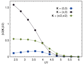
Figure 6: (Color online) The quantity $\beta G({\bf K},\frac{\beta}{2})$ in the different DCA momentum sectors ${\bf K}$ in the 8-site DCA approach at $T/t=1/12$. The values of $\beta G({\bf K},\frac{\beta}{2})$ at ${\bf K}=(\pi,\pi)$ are the same as those at ${\bf K}=(0,0)$. The error bars are smaller than symbol sizes. These results are comparable with those obtained from the interaction-expansion CT-QMC approach in Ref. Gull2009, .

In order to study the Mott behavior in 8-site DCA in more detail, we present in Fig. 5 the real part of the self-energy ${\rm Re}(\Sigma({\bf K},\omega))$ as a function of real frequency $\omega/t$ for $U/t=4.0$ and $5.2$ at $T/t=1/12$. The real and imaginary parts of the self-energy give the energy shift and the spectral broadening, respectively, of the one-electron spectrum due to the interaction $U/t$. In Fig. 5 (a) for $U/t=4.0$ where the spectral function shows a pseudo-gap, the real parts of the self-energy ${\rm Re}(\Sigma({\bf K},\omega))$ at ${\bf K}=(0,0)$ and $(\pi,\pi)$ remain finite below and above the Fermi level, respectively, indicating the shift of the pole positions of the one-electron spectrum. At ${\bf K}=(0,\pi)$ and $(\pi/2,\pi/2)$ ${\rm Re}(\Sigma({\bf K},\omega))$ shows a positive slope with negative value of quasiparticle weight and the corresponding ${\rm Im}(\Sigma({\bf K},\omega))$ (not shown) exhibits a peak around the Fermi level, indicating the appearance of a non-Fermi liquid. This non-Fermi-liquid behavior is the sign of the Mott gap beginning to form. In Fig. 5 (b) the $U/t=5.2$ case is presented. It is known that, in the Mott insulating state, the self-energy has a pole-like structure of the form

$$\Sigma(\omega)\propto\frac{1}{\omega-\triangle+i\gamma},$$ (50)

where the damping $\gamma$ is small, and $\triangle$ is the position of the pole Lin2009 . We observe that while the ${\rm Re}(\Sigma({\bf K},\omega))$ at ${\bf K}=(0,\pi)$ and $(\pi/2,\pi/2)$ for $\omega\rightarrow 0$ shows a pole-like structure indicating the Mott insulating state, the pole in the ${\rm Re}(\Sigma({\bf K},\omega))$ at ${\bf K}=(0,0)$ and $(\pi,\pi)$ lies above and below Fermi level, respectively.

In Fig. 6 we show $\beta G({\bf K},\frac{\beta}{2})$ as a function of $U/t$ at $T/t=1/12$. When the interaction $U/t$ is turned on, the values of $\beta G({\bf K},\frac{\beta}{2})$ at ${\bf K}=(0,0)$ increase until $U/t=3.6$ due to spectral weight transfer caused by electronic correlations, and a metallic behavior is seen in the ${\bf K}=(0,0)$ sector in the intermediate interaction strength regions. When the interaction becomes strong, the gap opens and $\beta G({\bf K},\frac{\beta}{2})$ goes to zero. In the ${\bf K}=(0,\pi)$ sector $\beta G({\bf K},\frac{\beta}{2})$ decreases monotonously and goes to zero at $U/t=5.6$. In the ${\bf K}=(\frac{\pi}{2},\frac{\pi}{2})$ sector, the values of $\beta G({\bf K},\frac{\beta}{2})$ remain nearly constant up to $U/t=3.0$. Beyond $U/t=3.0$, they decrease and the gap opens completely around $U/t=5.6$.

Finally, we compare the results in Fig. 6 to those in Fig. 8 of Ref. Gull2009, calculated within the CT-QMC approach. The behavior at ${\bf K}=(0,\pi)$ in both SCA and CT-QMC approaches is qualitatively the same, even though the critical interactions $U_{c}/t$ are different. The main difference between these two results is in the ${\bf K}=(\frac{\pi}{2},\frac{\pi}{2})$ sector. The CT-QMC results indicate a first-order transition with a discontinuous behavior of $\beta G({\bf K},\frac{\beta}{2})$ at the critical interaction $U_{c}/t$, while the SCA results show a continuous transition with a smooth decrease of $\beta G({\bf K},\frac{\beta}{2})$. We think that this discrepancy between the two approaches also comes from the approximation that the dynamical fluctuations are frozen in the SCA method.

III.2 Orbital-selective phase transitions in the two- orbital dynamical mean field theory

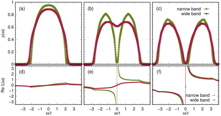
Figure 7: (Color online) The density of states $\rho(\omega)$ and real part of the self-energy ${\rm Re}(\Sigma(\omega))$ for (a) and (d) $U/t_{2}=2.0$, (b) and (e) 2.8, and (c) and (f) 3.6 at $T/t_{2}=1/12.0$, respectively. The bandwidths for narrow and wide orbitals on the Bethe lattice are $W_{1}=2.56$ ($t_{1}=0.8$) and $W_{2}=4.0$ ($t_{2}=1.0$), respectively. The metal, orbital-selective phase, and Mott insulator are present in (a), (b), and (c), respectively.

The orbital-selective phase transition (OSPT), where metallic behavior is seen in the wide band while a metal-insulator transition is observed in narrow band, has been intensively studied in model systems as well as real materials during the last ten years Anisimov2002 ; Koga2004 ; Knecht2005 ; Liebsch2005 ; Inaba2005 ; Biermann2005 ; Bouadim2009 ; Lee2010 ; Lee2011 ; Lee2012 . We study the anisotropic two-orbital Hubbard model with a narrow bandwidth of $W_{1}=2.56$ ($t_{1}=0.8$) for the first orbital and a wide bandwidth of $W_{2}=4$ ($t_{2}=1.0$) for the second orbital at half-filling on the Bethe lattice using single-site DMFT. The interaction part of the Hamiltonian is given by Eq. (16) with $U^{\prime}=\frac{U}{2}$ and $J_{z}=\frac{U}{4}$. The density of states $\rho(\omega)$ in both orbitals obtained with the SCA are shown in Fig. 7 (a)-(c). Metallic behavior in both bands is observed for the weak coupling strength $U/t_{2}=2.0$ in Fig. 7 (a). As the interaction $U/t$ increases, an orbital selective phase transition behavior is present in the intermediate regions for $U/t_{2}=2.8$ (see Fig. 7 (b)). Finally, insulating states in both orbitals are seen in the strong-coupling region for $U/t_{2}=3.6$ in Fig. 7 (c). We also present the real part of the self-energy ${\rm Re}(\Sigma(\omega))$ as a function of real frequency $\omega/t$ in Figs. 7 (d)-(f). As discussed for the 8-site DCA results, the Mott insulating state is related to a polelike structure in the self-energy as in Eq. (50). For $U/t_{2}=2.0$ ${\rm Re}(\Sigma(\omega))$ in both orbitals is small (Fig. 7 (d)). Increasing $U/t$ to $2.8$ we observe that ${\rm Re}(\Sigma(\omega))$ in the narrow-band orbital becomes large near the Fermi level (Fig. 7 (e)) while it retains its small value for the wide-band orbital (OSPT region). Finally for $U/t_{2}=3.6$, both self-energies show poles at $\omega/t=0$, indicating the Mott insulating behavior in both orbitals.

In the following we compare the critical values of the interaction strength obtained from the SCA and HF-QMC calculations in the case of band widths of $W_{1}=2$ (narrow band) and $W_{2}=4$ (wide band). The critical values in the HF-QMC approach are given as $U_{c_{1}}/t_{2}=2.0$ and $U_{c_{2}}/t_{2}=2.8$ in narrow and wide bands, respectively Knecht2005 . Our SCA results show the critical values $U_{c_{1}}/t_{2}=2.0$ and $U_{c_{2}}/t_{2}=3.2$ from the analysis of the Green’s function in the Matsubara frequency space in good agreement with HF-QMC. We encounter though a causality problem if the difference between the band widths of narrow and wide orbitals is large.

IV SUMMARY

In summary, in this work we propose that the semiclassical approximation in combination with the Monte Carlo method can be used to study large clusters and multi-orbital systems and is easy to embed into DMFT and its cluster extensions. We investigate the single-orbital Hubbard model by the DCA(SCA) method with cluster sizes of $N_{c}=4$ and 8 and a two-orbital system by DMFT(SCA). The critical $U_{c}/t$ as well as $G(\frac{\beta}{2})$ as a function of $\omega$ are compared with existing DCA(CT-QMC) results. The critical interactions $U/t$ of SCA and CT-QMC approaches in both cases are in reasonable agreement. In the 8-site DCA cluster calculation, we analyze the spectral functions $A({\bf K},\omega)$ and self-energy at each momentum sector. The only difference between SCA and CT-QMC results is that the CT-QMC shows a discontinuous behavior of the spectral density in the ${\bf K}=(\frac{\pi}{2},\frac{\pi}{2})$ sector around the critical value of interactions, while the SCA exhibits smoothly decreasing behavior. We think that the reason for the discrepancy is that quantum fluctuations are frozen in the SCA approach. In the two-orbital DMFT(SCA) calculation, we observe the orbital selective phase transition as in previous studies performed with DMFT(HF-QMC) Knecht2005 . This method is rather powerful since it can be applied for problems where other impurity solvers remain computationally too expensive but one should be aware of possible causality problems in some cases.

V ACKNOWLEDGMENTS

We would like to thank Gang Li, Hartmut Monien and Claudius Gros for useful discussions. HL, HOJ and RV gratefully acknowledge financial support from the Deutsche Forschungsgemeinschaft through the grant FOR 1346. YZ is supported by National Natural Science Foundation of China (No. 11174219), Shanghai Pujiang Program (No. 11PJ1409900), Research Fund for the Doctoral Program of Higher Education of China (No. 20110072110044) and the Program for Professor of Special Appointment (Eastern Scholar) at Shanghai Institutions of Higher Learning.

References

- (1) A. Georges, G. Kotliar, W. Krauth, and M. J. Rozenberg, Rev. Mod. Phys. 68, 13 (1996).
- (2) G. Kotliar and D. Vollhardt, Phys. Today 57 53 (2004).
- (3) G. Kotliar, S. Y. Savrasov, K. Haule, V. S. Oudovenko, O. Parcollet, and C. A. Marianetti, Rev. Mod. Phys. 78, 865 (2006).
- (4) M. H. Hettler, A. N. Tahvildar-Zadeh, M. Jarrell, T. Pruschke, and H. R. Krishnamurthy, Phys. Rev. B 58, 7475(R) (1998).
- (5) T. Maier, M. Jarrell, T. Pruschke, and M. H. Hettler, Rev. Mod. Phys. 77, 1027 (2005).
- (6) M. Civelli, M. Capone, S. S. Kancharla, O. Parcollet, and G. Kotliar, Phys. Rev. Lett. 95, 106402 (2005).
- (7) Y. Z. Zhang and M. Imada, Phys. Rev. B 76, 045108 (2007).
- (8) S. Sakai, Y. Motome, and M. Imada, Phys. Rev. Lett. 102, 056404 (2009).
- (9) A. Liebsch and N. Tong, Phys. Rev. B 80, 165126 (2009).
- (10) M. Sentef, P. Werner, E. Gull, and A. P. Kampf, Phys. Rev. Lett. 107, 126401 (2011).
- (11) G. Sordi, P. Semon, K. Haule, and A.-M. S. Tremblay, Phys. Rev. Lett. 108, 216401 (2012).
- (12) L. F. Tocchio, H. Lee, H. O. Jeschke, R. Valenti, and C. Gros, Phys. Rev. B 87, 045111 (2013).
- (13) P. Werner, A. Comanac, L. de’Medici, M. Troyer, and A. J. Millis, Phys. Rev. Lett. 97, 076405 (2006).
- (14) P. Werner and A. J. Millis, Phys. Rev. B 74, 155107 (2006).
- (15) A. N. Rubtsov, V. V. Savkin, and A. I. Lichtenstein, Phys. Rev. B 72, 035122 (2005).
- (16) E. Gull, A. Millis, A. I. Lichtenstein, A. N. Rubtsov, M. Troyer, and P. Werner, Rev. Mod. Phys. 83, 349 (2011).
- (17) J. E. Hirsch, Phys. Rev. B 31, 4403 (1985)
- (18) J.E. Hirsch and R. M. Fye, Phys. Rev. Lett. 56, 2521 (1986).
- (19) E. Khatami, C.R. Lee, Z.J. Bai, R. T. Scalettar, and M. Jarrell, Phys. Rev. E 81, 056703 (2010).
- (20) R. Blankenbecler, D. J. Scalapino, and R. L. Sugar, Phys. Rev. D 24, 2278 (1981).
- (21) S. Okamoto, A. Fuhrmann, A. Comanac, and A. J. Millis, Phys. Rev. B 71, 235113 (2005).
- (22) A. Fuhrmann, S. Okamoto, H. Monien, and A. J. Millis, Phys. Rev. B 75, 205118 (2007).
- (23) H. Lee, G. Li, and H. Monien, Phys. Rev. B 78, 205117 (2008).
- (24) X. Wang, E. Gull, L. de’Medici, M. Capone, and A. J. Millis, Phys. Rev. B 80, 045101 (2009).
- (25) E. Gull, P. Werner, A. Millis, and M. Troyer Phys. Rev. B 76, 235123 (2007).
- (26) Within the semiclassical approximation the auxiliary field is independent of the imaginary time and this hinders the existence of Fermi liquid behavior.
- (27) E. Gull, P. Werner, X. Wang, M. Troyer, and A. J. Millis, Europhys. Lett. 84, 37009 (2008).
- (28) E. Gull, O. Parcollet, P. Werner, and A. J. Millis, Phys. Rev. B 80, 245102 (2009).
- (29) S. Moukouri and M. Jarrell, Phys. Rev. Lett. 87, 167010 (2001).
- (30) B. Kyung, J. S. Landry, D. Poulin, and A.-M. S. Tremblay, Phys. Rev. Lett. 90, 099702 (2003).
- (31) K. Haule and G. Kotliar, Phys. Rev. B 76, 104509 (2007).
- (32) C. Lin and A. J. Millis, Phys. Rev. B 79, 205109 (2009).
- (33) Note that and become identical as the temperature approaches zero.
- (34) V. I. Anisimov, I. A. Nekrasov, D. E. Kondakov, T. M. Rice, and M. Sigrist, Eur. Phys. J. B 25, 191 (2002).
- (35) A. Koga, N. Kawakami, T. M. Rice, and M. Sigrist, Phys. Rev. Lett. 92, 216402 (2004).
- (36) C. Knecht, N. Blumer, and P. G. J. van Dongen, Phys. Rev. B 72, 081103 (2005).
- (37) A. Liebsch, Phys. Rev. Lett. 95, 116402 (2005).
- (38) K. Inaba, A. Koga, S.-I. Suga, and N. Kawakami, Phys. Rev. B 72, 085112 (2005).
- (39) S. Biermann, L. de’Medici, and A. Georges, Phys. Rev. Lett. 95, 206401 (2005).
- (40) K. Bouadim, G. G. Batrouni, and R. T. Scalettar, Phys. Rev. Lett. 102, 226402 (2009).
- (41) H. Lee, Y. Z. Zhang, H. O. Jeschke, R. Valentí, and H. Monien, Phys. Rev. Lett. 104, 026402 (2010).
- (42) H. Lee, Y. Z. Zhang, H. O. Jeschke, and R. Valentí, Phys. Rev. B 84, 020401(R) (2011).
- (43) G. Lee, H. S. Ji, Y. Kim, C. Kim, K. Haule, G. Kotliar, B. Lee, S. Khim, K. H. Kim, K. S. Kim, K-S. Kim, and J. H. Shim, Phys. Rev. Lett. 109, 177001 (2012).