Pulse profiles from thermally emitting neutron stars

Abstract

The problem of computing the pulse profiles from thermally emitting spots on the surface of a neutron star in general relativity is reconsidered. We show that it is possible to extend Beloborodov (2002) approach to include (multiple) spots of finite size in different positions on the star surface. Results for the pulse profiles are expressed by comparatively simple analytical formulas which involve only elementary functions.

1. Introduction

X-ray emission from isolated neutron stars (NSs), first detected in radio pulsars (PSRs), is now increasingly observed in other classes of sources, most of which are radio-silent or have radio properties much at variance with those of PSRs. They include the thermally emitting NSs (XDINSs; e.g. Turolla, 2009), the central compact objects in supernova remnants (CCOs; e.g De Luca, 2008), the magnetar candidates (SGRs and AXPs; e.g. Mereghetti, 2008; Rea & Esposito, 2011) and the rotating radio transients (RRaTs; e.g. Burke-Spolaor, 2012).

With the exception of some PSRs, the X-ray emission of which is dominated by a non-thermal component of magnetospheric origin, the spectra of all other X-ray emitting, isolated NSs exhibit one (or more) thermal component which, most probably, originates at the star surface. Since pulsations are observed, thermal X-ray photons come either from a localized, heated region, like in SGRs/AXPs and PSRs, or from the entire cooling surface with an inhomogeneous temperature distribution, like in XDINSs. In this respect the analysis of the observed pulse profiles in different energy bands is bound to reveal much on the surface thermal map of the NS, on the physical size and position of the emitting regions(s) in particular (e.g. Zane & Turolla, 2006; Albano et al., 2010).

The problem of modelling the pulse profiles of a rotating, thermally emitting NS, including the effects of gravitational ray bending, is an old one and has been thoroughly addressed in the literature (e.g. Pechenick, Ftaclas & Cohen, 1983; Page, 1995; Page & Sarmiento, 1996; Psaltis, Özel & DeDeo, 2000; Beloborodov, 2002; Zane & Turolla, 2006). In particular, in their classic paper Pechenick, Ftaclas & Cohen (1983) analyzed the emission from two antipodal, uniform, circular caps. Although their approach contains no inherent complexity, the treatment of photon propagation in a Schwarzschild spacetime leads to elliptic integrals and requires numerical evaluation. In general, resorting to a numerical approach is unavoidable every time a continuous surface temperature distribution, anisotropic emission and/or an arbitrary shape of the emission regions have to be accounted for. However, Beloborodov (2002), by means of a clever approximation, has shown that simple, analytical expressions can be derived for the pulse profiles in full general relativity (Schwarzschild spacetime) for point-like spots.

In this paper we make use of Beloborodov (2002) approximate treatment to extend his analysis to the case of finite, uniform, circular spots. Our results are valid for an arbitrary number of spots, regardless of their size, temperature and mutual position on the star surface (e.g. two different, non-antipodal caps). Some more complex emission geometries (like a cap surrounded by a corona) can also be easily accommodated. The expression for the total observed flux is analytical and this makes our approach both simple and fast for the evaluation and comparison of pulse profiles with observations.

2. Observed flux

Let us consider a surface element $dS$ on a neutron star of radius $R$ and mass $M$ and let us assume that the Schwarzschild solution correctly describes the spacetime outside the star (in the following $R_{S}=2GM/c^{2}$ is the Schwarzschild radius). Let us further introduce a spherical coordinate system, $(r,\,\theta,\,\phi)$, centered on the star in such a way that the polar axis coincides with the line-of-sight (LOS; unit vector $\mathbf{\hat{l}}$). The distance to the observer is $D\gg R$.

Because photon trajectories are not straight lines, the ray from $dS=R^{2}\sin\theta d\theta d\phi$ which reaches the observer leaves the surface, with respect to the local normal, at an angle $\alpha\neq\theta$ (see Figure 1). The relation between $\alpha$ and $\theta$ is given, implicitly, by the two equations

$$\theta=\int_{R}^{\infty}\frac{dr}{r^{2}}\left[\frac{1}{b^{2}}-\frac{1}{r^{2}}\left(1-\frac{R_{S}}{r}\right)\right]^{-1/2}$$ (1)

$$\sin\alpha=\frac{b}{R}\left(1-\frac{R_{S}}{R}\right)^{1/2}\,,$$ (2)

where $b$ is the ray impact parameter Beloborodov (2002).

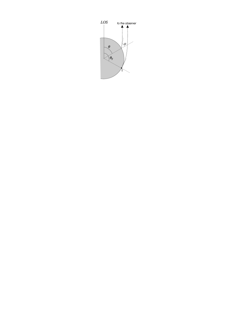
Figure 1.— A schematic view of ray propagation. The angles $\theta$, $\alpha$ and $\theta_{F}$ are also shown.

The (monochromatic) flux $dF_{\nu}$ from $dS$ detected by the observer is then

$$dF_{\nu}=\left(1-\frac{R_{S}}{R}\right)I_{\nu}\cos\alpha\left(\frac{d\cos\alpha}{d\cos\theta}\right)\frac{dS}{D^{2}}\,.$$ (3)

where $\nu$ is the photon frequency and $I_{\nu}$ the specific intensity, both measured by the static observer at $r=R$. The total flux is obtained by integrating the previous expression over the visible part of the emitting region, $S_{V}$. If the emission is Planckian at the local (uniform) temperature $T$, $I_{\nu}=B_{\nu}(T)$ and this results in

$$F_{\nu}=\left(1-\frac{R_{S}}{R}\right)B_{\nu}(T)\int_{S_{V}}\cos\alpha\left(\frac{d\cos\alpha}{d\cos\theta}\right)\frac{dS}{D^{2}}\,.$$ (4)

In Newtonian gravity it is $\alpha=\theta$ and the flux is simply proportional to the area of the visible emitting region projected in the plane of the sky.

Beloborodov (2002) found that a simple, approximate expression can be used to link $\alpha$ and $\theta$, without the need to solve (numerically) eqs. (1) and (2),

$$1-\cos\alpha=(1-\cos\theta)\left(1-\frac{R_{S}}{R}\right)\,.$$ (5)

Eq. (5) is remarkably accurate and produces a fractional error $\lesssim 3\%$ for $R\gtrsim 3R_{S}$. Substituting $\cos\alpha$ and $d\cos\alpha/d\cos\theta$ into eq. (4), one obtains

$$F_{\nu}=\left(1-\frac{R_{S}}{R}\right)^{2}B_{\nu}(T)\int_{S_{V}}\left[\frac{R_{S}}{R}+\left(1-\frac{R_{S}}{R}\right)\cos\theta\right]\frac{dS}{D^{2}}\,.$$ (6)

The flux is, then, expressed by the sum of two contributions, the first proportional to the surface area and the second to the projected area of the visible part of the emitting region. The latter, apart for the factor $(1-R/R_{S})$, is the analogue of the Newtonian expression, while the former is a purely relativistic correction. The problem of computing the flux, once the geometry is fixed, is therefore reduced to that of determining $S_{V}$ and evaluating the two integrals

$$I_{p}=\int_{S_{V}}\cos\theta\sin\theta\,d\theta d\phi\,,\quad I_{s}=\int_{S_{V}}\sin\theta\,d\theta d\phi\,.$$ (7)

2.1. Single circular spot

In order to proceed further, we consider first the simplest case, in which the emitting region is a circular cap of semi-aperture $\theta_{c}$ with its center at $(R,\,\theta_{o},\,0)$. For the sake of simplicity, and also because this is the most common occurrence, we consider only the case $\theta_{c}\leq\pi/2$. Moreover, we restrict to $0\leq\theta_{o}\leq\pi$, since the case $\pi\leq\theta_{o}\leq 2\pi$ is reduced to the previous one upon the substitution $\theta_{o}\to 2\pi-\theta_{o}$, given the axial symmetry around the LOS.

The $\phi$-integral in both $I_{p}$ and $I_{s}$ is immediate. By denoting with $\phi_{b}(\theta)$ the cap boundary ($0\leq\phi_{b}\leq\pi$), it is

$$I_{p}=2\int_{\theta_{\mathrm{min}}}^{\theta_{\mathrm{max}}}\cos\theta\sin\theta\phi_{b}(\theta)\,d\theta\,,\quad I_{s}=2\int_{\theta_{\mathrm{min}}}^{\theta_{\mathrm{max}}}\sin\theta\phi_{b}(\theta)\,d\theta\,,$$ (8)

where $\theta_{\mathrm{min}}$, $\theta_{\mathrm{max}}$ are the limiting values of the co-latitude, which are discussed below.

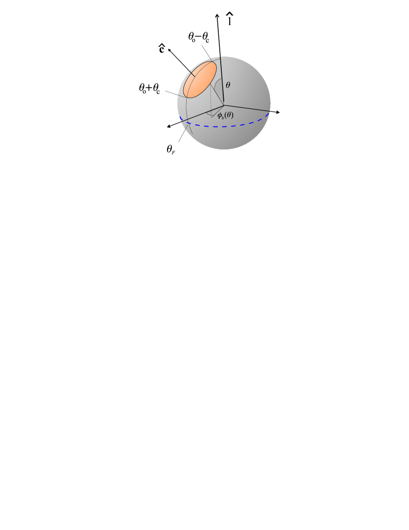
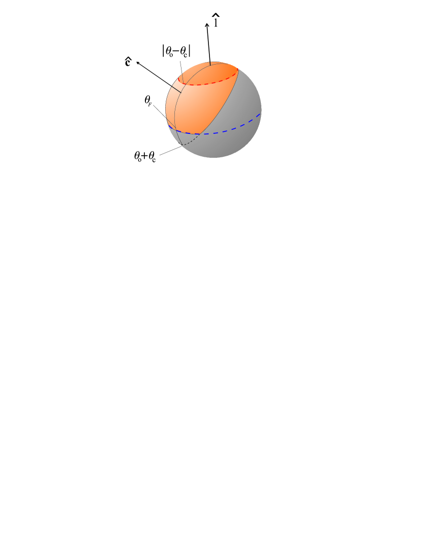
Figure 2.— Geometry for a single spot; the visible part is in orange and the terminator is marked by the blue, dashed line. (Left) The spot is fully into view and $\theta_{o}-\theta_{c}>0$. (Right) The spot is partially into view and $\theta_{o}-\theta_{c}<0$; the darker part bounded by the dashed orange line is the region $0\leq\theta\leq|\theta_{o}-\theta_{c}|$ (see text).

The function $\phi_{b}$ can be readily found noticing that a generic point on the cap boundary has coordinates $(R\,,\theta,\,\phi_{b})$. In a spherical coordinate system with the polar axis coincident with the cap axis (unit vector $\mathbf{\hat{c}}$), its coordinates are $(R\,,\Theta\equiv\theta_{c},\,\Phi)$; the latter system is rotated by an angle $\theta_{o}$ with respect to the former around an axis perpendicular to the $\mathbf{\hat{l}}$–$\mathbf{\hat{c}}$ plane. By exploiting the transformation between the (cartesian) coordinates in the two systems, one gets

$$\cos\theta=\cos\theta_{o}\cos\theta_{c}-\sin\theta_{o}\sin\theta_{c}\cos\Phi\,,$$ (9)

$$\sin\theta\cos\phi_{b}=\cos\theta_{o}\sin\theta_{c}\cos\Phi+\sin\theta_{o}\cos\theta_{c}\,.$$ (10)

Solving the second for $\cos\Phi$ and substituting into the first one, one finally obtains

$$\cos\phi_{b}=\frac{\cos\theta_{c}-\cos\theta_{o}\cos\theta}{\sin\theta_{o}\sin\theta}\,;$$ (11)

$\cos\phi_{b}$ is actually related to the function $h$ introduced by Pechenick, Ftaclas & Cohen (1983). It is immediate to verify that it is $-1\leq\cos\phi_{b}\leq 1$, and hence $\phi_{b}$ is defined, in the range $|\theta_{o}-\theta_{c}|<\theta<\min{[\theta_{o}+\theta_{c},2\pi-(\theta_{o}+\theta_{c})]}$, since it must be, by definition, $0\leq\theta\leq\pi$. It is important to notice that the $\theta$-range in which it is possible to define $\cos\phi_{b}$ is not sufficient to cover the entire cap when the LOS intersects the cap itself: this occurs either for $\theta_{o}-\theta_{c}<0$ or $\theta_{o}+\theta_{c}>\pi$. Since it is $0<\theta_{c}\leq\pi/2$ by assumption and disregarding visibility, there is just one intersection, at $\theta=0$ or $\pi$. In these cases the cap is fully covered only by adding the range $0\leq\theta\leq|\theta_{o}-\theta_{c}|$ or $2\pi-(\theta_{o}+\theta_{c})\leq\theta\leq\pi$, respectively. This accounts for the missing surface which is itself a circular cap, perpendicular to the LOS, where $\phi$ spans the entire range $[0\,,2\pi]$ (see fig. 2). Accordingly, the definition of $\phi_{b}(\theta)$ can be continuously extended as

$$\phi_{b}(\theta)=\begin{cases}\arccos{\displaystyle\left[\frac{\cos\theta_{c}-\cos\theta_{o}\cos\theta}{\sin\theta_{o}\sin\theta}\right]}&|\theta_{o}-\theta_{c}|<\theta<\min{[\theta_{o}+\theta_{c},2\pi-(\theta_{o}+\theta_{c})]}\cr\cr\pi&0\leq\theta\leq|\theta_{o}-\theta_{c}|\quad\mathrm{if}\ \theta_{o}-\theta_{c}\leq 0\cr&2\pi-(\theta_{o}+\theta_{c})\leq\theta\leq\pi\quad\mathrm{if}\ \theta_{o}+\theta_{c}\geq\pi\cr\end{cases}$$ (12)

to include all cases.

At each visible point of the star surface it has to be $\cos\alpha\geq 0$, and the terminator lies precisely at $\alpha=\pi/2$. From eq. (5) it follows that the terminator co-latitude is given by

$$\cos\theta_{F}=\left(1-\frac{R}{R_{S}}\right)^{-1};$$ (13)

it is $\cos\theta_{F}\leq 0$ and $\theta_{F}\geq\pi/2$, as expected, since relativistic effects bring more than half the sphere into view.

In the case the cap is entirely visible, i.e. it does not intersect the terminator, its co-latitude is in the range $\theta_{\mathrm{min}}=\max{(0,\theta_{o}-\theta_{c})}\leq\theta\leq\theta_{\mathrm{max}}=\min{[2\pi-(\theta_{o}+\theta_{c}),\theta_{o}+\theta_{c}]}$. The presence of the terminator (at $\pi/2\leq\theta_{F}<\pi$) is easily accounted for by replacing $\theta_{\mathrm{min}}$ ($\theta_{\mathrm{max}}$), as defined above, with $\theta_{F}$ every time it is $\theta_{F}<\theta_{\mathrm{min}}$ ($\theta_{F}<\theta_{\mathrm{max}}$). Summarizing, it is

$$\theta_{\mathrm{min}}=\min{[\max{(0,\theta_{o}-\theta_{c})},\theta_{F}]}$$ (14)

and

$$\theta_{\mathrm{max}}=\min{(\theta_{0}+\theta_{c},\theta_{F})}\,.$$ (15)

Turning to the evaluation of $I_{p,s}$, both integrals become trivial for $\phi_{b}=\pi$ and yield

$$I_{p}=2\int_{\theta_{1}}^{\theta_{2}}\pi\cos\theta\sin\theta\,d\theta=\pi(\sin^{2}\theta_{2}-\sin^{2}\theta_{1})\,,\quad I_{s}=2\int_{\theta_{1}}^{\theta_{2}}\pi\sin\theta\,d\theta=2\pi(\cos\theta_{2}-\cos\theta_{1})$$ (16)

for any pair of angles $\theta_{1}\,,\theta_{2}$. In the opposite case, the two indefinite integrals

$$I_{1}=2\int\cos\theta\sin\theta\arccos\left[\frac{\cos\theta_{c}-\cos\theta_{o}\cos\theta}{\sin\theta_{o}\sin\theta}\right]\,d\theta\,,$$ (17)

and

$$I_{2}=2\int\sin\theta\arccos\left[\frac{\cos\theta_{c}-\cos\theta_{o}\cos\theta}{\sin\theta_{o}\sin\theta}\right]\,d\theta$$ (18)

have to be calculated. It turns out that $I_{1,2}$ can be evaluated analytically in terms of elementary functions (see the Appendix for more details)

$$I_{1} = \sin^{2}\theta\arccos\left[\frac{\cos\theta_{c}-\cos\theta_{o}\cos\theta}{\sin\theta_{o}\sin\theta}\right]-\sin^{2}\theta_{c}\cos\theta_{o}\arcsin\left[\frac{\cos\theta-\cos\theta_{o}\cos\theta_{c}}{\sin\theta_{o}\sin\theta_{c}}\right]$$ (20)

$$-\cos\theta_{c}\sqrt{-\left[\cos\theta-\cos(\theta_{o}+\theta_{c})\right]\left[\cos\theta-\cos(\theta_{o}-\theta_{c})\right]}$$

and

$$I_{2} = -2\cos\theta\arccos\left[\frac{\cos\theta_{c}-\cos\theta_{o}\cos\theta}{\sin\theta_{o}\sin\theta}\right]+2\cos\theta_{c}\arcsin\left[\frac{\cos\theta-\cos\theta_{o}\cos\theta_{c}}{\sin\theta_{o}\sin\theta_{c}}\right]$$ (23)

$$+\mathrm{sign}\left(\theta_{o}+\theta_{c}-\pi\right)\arcsin\left[\frac{(\cos\theta_{o}\cos\theta_{c}+1)\cos\theta+\sin^{2}\theta_{o}-\cos^{2}\theta_{c}-\cos\theta_{o}\cos\theta_{c}}{(1+\cos\theta)|\sin\theta_{o}\sin\theta_{c}|}\right]$$

$$-\mathrm{sign}\left(\theta_{o}-\theta_{c}\right)\arcsin\left[\frac{(\cos\theta_{o}\cos\theta_{c}-1)\cos\theta+\sin^{2}\theta_{o}-\cos^{2}\theta_{c}-\cos\theta_{o}\cos\theta_{c}}{(1-\cos\theta)|\sin\theta_{o}\sin\theta_{c}|}\right]\,,$$

where the arbitrary constant was set to zero. It is then $I_{p,s}=I_{1,2}(\theta_{max})-I_{1,2}(\theta_{min})$. We note that $I_{1,2}$ take a simple form for $\theta=\theta_{o}\pm\theta_{c}$. In particular, if the cap is fully into view (see Figure 2, left), it is $I_{p}=\pi\cos\theta_{o}\sin^{2}\theta_{c}$ and $I_{s}=2\pi(1-\cos\theta_{c})$, as it follows also from geometrical considerations. The complete form of eqs. (20) and (23) is actually required only when evaluating the integrals at $\theta_{F}$.

The flux (eq. [6]) is finally written as

$$F_{\nu}=\left(1-\frac{R_{S}}{R}\right)^{2}B_{\nu}(T)A_{\mathrm{eff}}(\theta_{c},\theta_{o})\,,$$ (24)

where we introduced the “effective” area

$$A_{\mathrm{eff}}(\theta_{c},\theta_{o})=R^{2}\left[\frac{R_{S}}{R}I_{s}+\left(1-\frac{R_{S}}{R}\right)I_{p}\right]\,.$$ (25)

2.2. Multiple spots and other geometries

Having computed the flux seen by a distant observer for a single circular spot, it is straightforward to generalize the result to an arbitrary number of spots. We stress that this is possible because, using Beloborodov’s approximation, the flux is proportional to the “effective” area of the cap, $A_{\mathrm{eff}}$, introduced in the previous section. Although we impose no restrictions on the parameters, the assumption that the spots do not intersect is understood. For the sake of simplicity, here we consider just two circular, uniform caps with semi-aperture $\theta_{c,i}$, and temperature $T_{i}$ ($i=1,\,2$). Let us further assume that the spots are aligned, in the sense that their centers lie on the same meridian (the more general case of misaligned caps will be discussed in the next section), and let $\theta_{d,2}$ be the relative angular displacement of second one with respect to the first, the center of which is at $\theta_{o}$ (of course it is $\theta_{d,1}=0$). The spot centers are then at $\theta_{o,i}=\theta_{o}+\theta_{d,i}$ and the total flux can be calculated by simply adding the two contributions

$$F_{\nu}^{\mathrm{TOT}}=\left(1-\frac{R_{S}}{R}\right)^{2}\left[B_{\nu}(T_{1})A_{\mathrm{eff}}(\theta_{c,1},\theta_{o})+B_{\nu}(T_{2})A_{\mathrm{eff}}(\theta_{c,2},\theta_{o}+\theta_{d,2})\right]\,.$$ (26)

The case of a two-temperature cap, i.e. a cap at $T_{1}$ surrounded by a circular corona at $T_{2}$, is treated much in the same way by subtracting from the larger cap the contribution of the inner spot and adding the latter at the proper temperature

$$F_{\nu}^{\mathrm{TOT}}=\left(1-\frac{R_{S}}{R}\right)^{2}\left\{B_{\nu}(T_{2})\left[A_{\mathrm{eff}}(\theta_{c,2},\theta_{o})-A_{\mathrm{eff}}(\theta_{c,1},\theta_{o})\right]+B_{\nu}(T_{1})A_{\mathrm{eff}}(\theta_{c,1},\theta_{o})\right\}\,.$$ (27)

With the aid of the previous expressions more configurations can be modelled. In particular, for a NS with a thermal map made of two (antipodal) caps at $T_{1}$ while the rest of the surface is at $T_{2}$, one obtains the flux by using twice eq. (27) with $\theta_{c,2}=\pi/2$, the second time replacing $\theta_{o}$ with $\theta_{o}+\pi$, and summing the two contributions. The similar case of a single cap at $T_{1}$ is handled by summing the flux given by eq. (27) with $\theta_{c,2}=\pi/2$ and that of eq. (24), with $\theta_{c}=\pi/2$, $\theta_{o}\to\theta_{o}+\pi$.

2.3. Pulse profiles

In order to compute pulse profiles we consider first the case of a single spot. Let $\mathbf{\hat{r}}$ be a unit vector parallel to the rotation axis and $\Omega$ the star angular velocity, $\Omega=2\pi/P$ where $P$ is the spin period. Observed periods in X-ray emitting INSs are in the range $\approx 0.1$–10 s, so the assumption of Schwarzschild spacetime previously introduced is fully justified. We also introduce the angles $\chi$, $\xi$ between the LOS, the cap axis and the rotation axis, respectively, i.e. $\cos\chi=\mathbf{\hat{r}}\cdot\mathbf{\hat{l}}$ and $\cos\xi=\mathbf{\hat{r}}\cdot\mathbf{\hat{c}}$.

Since the cap co-rotates with the star, the vector $\mathbf{\hat{c}}$ rotates around $\mathbf{\hat{r}}$, keeping $\xi$ constant. This implies that $\theta_{o}$ changes in time. Introducing the rotational phase $\gamma=\Omega t+\gamma_{0}$ ($\gamma_{0}$ is an arbitrary initial phase), from simple geometrical considerations it follows that

$$\cos\theta_{o}=\cos\chi\cos\xi-\sin\chi\sin\xi\cos\gamma\,.$$ (28)

Eq. (24) then provides the phase-resolved spectrum once the previous expression is used for $\cos\theta_{o}$. The pulse profile in a given energy band is immediately obtained integrating over frequencies. Since $\int_{0}^{\infty}B_{\nu}(T)\,d\nu=\sigma T^{4}/\pi$ ($\sigma$ is the Stefan-Boltzmann constant), the pulse profile in the $[\nu_{1},\,\nu_{2}]$ range is

$$F(\nu_{1},\nu_{2})=\left(1-\frac{R_{S}}{R}\right)^{2}C(\nu_{1},\nu_{2})\frac{\sigma T^{4}}{\pi}A_{\mathrm{eff}}(\theta_{c},\theta_{o})\,,$$ (29)

where $C(\nu_{1},\nu_{2})=(\pi/\sigma T^{4})\int_{\nu_{1}}^{\nu_{2}}B_{\nu}(T)\,d\nu$. Similar expressions hold for other geometries.

Figure 3.— (Left) Normalized flux as a function of phase for a single spot of semi-aperture $\theta_{c}=40^{\circ}$ and different values of $\chi$ and $\xi$; (right) same, but for $\theta_{c}=3^{\circ}$.

Some examples are illustrated in Figure 3, 4 and 5 where the pulse profiles are shown for seven values of the angles $\chi,\,\xi$ in the range $[0^{\circ},\,90^{\circ}]$, step $15^{\circ}$. Because eq. (28) is invariant by exchanging $\chi$ and $\xi$, only the 28 pulse profiles which are actually diverse are shown. In all cases it is $M=1.4\,M_{\odot}$ and $R=15$ km ($R/R_{S}=3.6$), corresponding to $\theta_{F}=112^{\circ}$, and the pulse profiles refer to the bolometric flux (i.e. $C=1$), normalized to $(F_{\mathrm{max}}+F_{\mathrm{min}})/2$. Figure 3 shows the case of a single spot for $\theta_{c}=40^{\circ}$ (left) and $\theta_{c}=3^{\circ}$ (right), small enough to te treated as point-like (see §3). The pulse profiles for two equal, antipodal ($\theta_{d,2}=180^{\circ}$) spots are illustrated in Figure 4, again for $\theta_{c}=30^{\circ}$ (left) and $\theta_{c}=3^{\circ}$ (right).

Figure 4.— Same as in fig. 3, but for two equal, antipodal caps.

Figure 5 (left) refers to two non-antipodal ($\theta_{d,2}=120^{\circ}$), different ($\theta_{c,1}=30^{\circ}\,,\theta_{c,2}=45^{\circ}$, $kT_{1}=0.4$ keV, $kT_{2}=1$ keV) caps, while the right panel illustrates the same case, but with the second spot shifted in longitude by $45^{\circ}$. The latter is simply obtained by adding a constant phase-shift to $\gamma$ in eq. (28) when $\theta_{o}$ refers to the second spot.

Figure 5.— Same as in fig. 3, but for two different, non-antipodal caps on the same meridian (left) and with the second spot shifted in longitude by $45^{\circ}$ (right).

3. Discussion and conclusions

In this investigation we revisited the problem of computing the pulse profiles from thermally emitting spots on the surface of a neutron star in general relativity. Our goal has been to develop a simple approach which can be readily used for a quantitative comparison of models with observations. Beloborodov (2002), by means of a suitable approximation, was able to derive analytical expressions for the pulse profiles in full GR for point-like, equal, antipodal spots. However, if more realistic thermal configurations are to be accounted for, going beyond the point-like approximation becomes necessary. We have shown that it is possible to extend Beloborodov’s approach to include (multiple) spots of finite size in different positions on the star surface. Results for the pulse profiles are expressed by comparatively simple analytical formulas which involve only elementary functions.

A qualitative comparison between point-like and finite-size spots is provided by Figures 3 (single spot) and 4 (two equal, antipodal spots); since $\theta_{c}=0$ produces a vanishing flux, $\theta_{c}=3^{\circ}$ was used instead to simulate a (nearly) point-like spot (see below). Indeed, the pulse profiles in Figure 4 (right) appear very similar to those discussed by Beloborodov (2002, see his fig. 4) and the four “types” he introduced (class I, II, III, IV) are clearly recognizable. This is better seen in Figure 6 (right), where the pulsed fraction, defined as ${\mathrm{PF}}=(F_{max}-F_{min})/(F_{max}+F_{min})$, is shown as a function of $\chi$ and $\xi$, together with Beloborodov’s analytical result (his eq. [8]). The two sets of contours are nearly indistinguishable and the maximum pulsed fraction, equal to $(R-2R_{S})/(R+2R_{S})$ for point-like spots, is the same.

As expected, for larger caps the pulse shape changes, the “plateau” disappears and the pulsed fraction decreases (figure 4, left). Now the constant PF contours are quite different with respect to those of a point-like spot, as clearly shown in the left panel of figure 6. The maximal pulsed fraction is $\sim 30\%$ lower than $(R-2R_{S})/(R+2R_{S})$ for $\theta_{c}=40^{\circ}$. In general, we find that the point-like approximation is reliable up to $\theta_{c}\sim 5^{\circ}$.

Figure 6.— Contour plot for the pulsed fraction as a function of the two angles $\chi$ and $\xi$ (full lines) for two antipodal, equal spots with semi-aperture $40^{\circ}$ (left) and $3^{\circ}$ (right). The dashed contours show the analytical result and the rectangle bounded by the heavy lines (left panel) separates the five regions labelled I, II, III, IV (Beloborodov, 2002, see text).

Larger caps can be treated either using the approach described here or resorting to methods based on general relativistic ray-tracing. We believe that the former offers a number of advantages, since it involves no numerical integration, and allows for a great flexibility, so that diverse thermal configurations of the NS surface can be modeled. An obvious limitation is that only purely blackbody (or at any rate isotropic) emission can be treated. Despite this simple model is often successfully used in fitting the (thermal components) of X-ray spectra, emission from the cooling surface of isolated neutron stars is expected to be more complicated, e.g. because the star is covered by an atmosphere, or because the emissivity is strongly suppressed at energies below the electron plasma frequency if the surface layers are in condensed form (see e.g. Turolla, 2009, and references therein). Realistic emission models predict, to a different extent, an angular dependence of the emitted intensity. While anisotropy is modest for non-magnetized atmospheric models Zavlin, Pavlov & Shibanov (1996), it becomes substantial in magnetized atmospheres Pavlov, Shibanov, Ventura & Zavlin (1994), or in condensed surfaces Turolla, Zane & Drake (2004). In general, it would be impossible to compute analytically the analogues of $I_{1,2}$ (see §2.1) for a non-isotropic radiation field. We point out, however, that in case the intensity depends on the angle $\alpha$ only, i.e. $I_{\nu}=I_{\nu}(\theta)$ by using eq. (5), all the cosiderations presented in §2.1 still hold, although now numerical integration is required to obtain the pulse profiles. This, being the integral just over a single variable, $\theta$, adds only a modest complication and the present method has still advantages with respect to fully numerical ray-tracing. Clearly this is not the case if $I_{\nu}$ depends on both angles, $\alpha$ and the associated azimuth, since double integrals should be evaluated.

Appendix A Integrals evaluation

An integration by parts brings the first integral into the form

$$I_{1}=\sin^{2}\theta\arccos\left[\frac{\cos\theta_{c}-\cos\theta_{o}\cos\theta}{\sin\theta_{o}\sin\theta}\right]-\frac{1}{\sin\theta_{o}\sin\theta_{c}}\int\frac{\cos\theta_{o}-\cos\theta_{c}\mu}{\sqrt{1-\displaystyle{\left(\frac{\mu-\cos\theta_{o}\cos\theta_{c}}{\sin\theta_{o}\sin\theta_{c}}\right)^{2}}}}\,d\mu$$ (A1)

where $\mu=\cos\theta$. By introducing $z=(\mu-\cos\theta_{o}\cos\theta_{c})/(\sin\theta_{o}\sin\theta_{c})$, the previous expression becomes

$$I_{1}=\sin^{2}\theta\arccos\left[\frac{\cos\theta_{c}-\cos\theta_{o}\cos\theta}{\sin\theta_{o}\sin\theta}\right]-\sin^{2}\theta_{c}\cos\theta_{o}\int\frac{dz}{\sqrt{1-z^{2}}}+\cos\theta_{c}\sin\theta_{c}\sin\theta_{o}\int\frac{z\,dz}{\sqrt{1-z^{2}}}\,,$$ (A2)

which, after some trivial manipulations, yields eq. (20).

$I_{2}$ is handled in a similar way. After integrating by parts, one gets

$$I_{2}=-2\cos\theta\arccos\left[\frac{\cos\theta_{c}-\cos\theta_{o}\cos\theta}{\sin\theta_{o}\sin\theta}\right]+\frac{2}{\sin\theta_{o}\sin\theta_{c}}\int\frac{\mu(\cos\theta_{o}-\cos\theta_{c}\mu)}{1-\mu^{2}}\frac{d\mu}{\sqrt{1-\displaystyle{\left(\frac{\mu-\cos\theta_{o}\cos\theta_{c}}{\sin\theta_{o}\sin\theta_{c}}\right)^{2}}}}\,.$$ (A3)

Upon writing

$$\frac{\mu(\cos\theta_{o}-\cos\theta_{c}\mu)}{1-\mu^{2}}=\cos\theta_{c}+\frac{1}{2}\left(-\frac{\cos\theta_{o}+\cos\theta_{c}}{1+\mu}+\frac{\cos\theta_{o}-\cos\theta_{c}}{1-\mu}\right)\,,$$ (A4)

eq. (A3) can be cast as

$$I_{2} = -2\cos\theta\arccos\left[\frac{\cos\theta_{c}-\cos\theta_{o}\cos\theta}{\sin\theta_{o}\sin\theta}\right]+2\cos\theta_{c}\int\frac{dz}{\sqrt{1-z^{2}}}$$ (A7)

$$-\left(\cos\theta_{o}+\cos\theta_{c}\right)\int\frac{d\mu}{(\mu+1)\sqrt{-\mu^{2}+2\cos\theta_{c}\cos\theta_{o}\mu-\cos^{2}\theta_{c}-\cos^{2}\theta_{o}+1}}$$

$$-\left(\cos\theta_{o}-\cos\theta_{c}\right)\int\frac{d\mu}{(\mu-1)\sqrt{-\mu^{2}+2\cos\theta_{c}\cos\theta_{o}\mu-\cos^{2}\theta_{c}-\cos^{2}\theta_{o}+1}}\,.$$

The last two integrals in eq. (A7) are of the general type

$$\int\frac{dx}{(x+p)\sqrt{ax^{2}+bx+c}}=\frac{1}{\sqrt{bp-ap^{2}-c}}\arcsin\frac{(b-2ap)x-bp+2c}{(x+p)\sqrt{b^{2}-4ac}}$$ (A8)

($ap^{2}-bp+c<0\,,b^{2}-4ac>0\,;$ e.g. Prudnikov, Brychkov & Marichev 1992). Note, however, that the previous expression is valid only if $x+p>0$. If $x+p<0$, as in the last integral in eq. (A7) where $\mu-1<0$, a minus sign must be placed in front of the result. Making use of eq. (A8) and after some algebra, eq. (23) is finally recovered.

References

- Albano et al. (2010) Albano, A., Turolla, R., Israel, G.L., Zane, S., Nobili, L., & Stella, L. 2010, ApJ, 722, 788
- Beloborodov (2002) Beloborodov, A.M. 2002, ApJ, 566, L85
- Burke-Spolaor (2012) Burke-Spolaor, S. 2012, in Proceedings of IAU Symposium 291 Neutron Stars and Pulsars: Challenges and Opportunities after 80 years, van Leeuwen, J. ed. [eprint: arXiv:1212.1716]
- De Luca (2008) De Luca, A. 2008, in 40 Years of Pulsars: Millisecond Pulsars, Magnetars and More. AIP Conference Proceedings, 983, 311
- Pechenick, Ftaclas & Cohen (1983) Pechenick, K.R., Ftaclas, C., & Cohen, M.J. 1983, ApJ, 274, 846
- Mereghetti (2008) Mereghetti, S. 2008, A&A Review, 15, 225
- Page (1995) Page, D. 1995, ApJ, 442, 273
- Page & Sarmiento (1996) Page, D., & Sarmiento, A. 1996, ApJ, 473, 1067
- Pavlov, Shibanov, Ventura & Zavlin (1994) Pavlov, G.G., Shibanov, Yu.A., Ventura, J., & Zavlin, V.E. 1994, A&A, 289, 837
- Prudnikov, Brychkov & Marichev (1992) Prudnikov, A.P, Brychkov, Yu.A., & Marichev, O.I. 1992, Integrals and Series. I. Elementary Functions, Gordon & Breach (New York)
- Pavlov, Shibanov, Ventura & Zavlin (1994) Pavlov, G.G., Shibanov, Yu.A., Ventura, J., & Zavlin, V.E. 1994, A&A, 289, 837
- Psaltis, Özel & DeDeo (2000) Psaltis, D., Özel, F., & DeDeo, S. 2000, ApJ, 544, 390
- Rea & Esposito (2011) Rea, N., & Esposito, P. 2011, in “High-energy emission from pulsars and their systems”, proceedings of the Sant Cugat Forum on Astrophysics, Rea, N. & Torres, D.F. eds., Springer, Berlin, p. 247 [eprint: arXiv:1101.4472]
- Turolla (2009) Turolla, R. 2009, in Astrophysics and Space Science Library, Neutron Stars and Pulsars. Springer (Berlin), p. 357
- Turolla, Zane & Drake (2004) Turolla, R, Zane, S., & Drake, J.J. 2004, ApJ, 603, 265
- Zane & Turolla (2006) Zane, S., & Turolla, R. 2006, MNRAS, 366, 727
- Zavlin, Pavlov & Shibanov (1996) Zavlin, V.E., Pavlov, G.G., & Shibanov, Yu.A. 1996, A&A, 315, 141