$\beta$-coalescents and stable Galton-Watson trees

Abstract.

Representation of coalescent process using pruning of trees has been used by Goldschmidt and Martin for the Bolthausen-Sznitman coalescent and by Abraham and Delmas for the $\beta(3/2,1/2)$-coalescent. By considering a pruning procedure on stable Galton-Watson tree with $n$ labeled leaves, we give a representation of the discrete $\beta(1+\alpha,1-\alpha)$-coalescent, with $\alpha\in[1/2,1)$ starting from the trivial partition of the $n$ first integers. The construction can also be made directly on the stable continuum Lévy tree, with parameter $1/\alpha$, simultaneously for all $n$. This representation allows to use results on the asymptotic number of coalescence events to get the asymptotic number of cuts in stable Galton-Watson tree (with infinite variance for the offspring distribution) needed to isolate the root. Using convergence of the stable Galton-Watson tree conditioned to have infinitely many leaves, one can get the asymptotic distribution of blocks in the last coalescence event in the $\beta(1+\alpha,1-\alpha)$-coalescent.

1. Introduction

1.1. Framework

The idea of constructing coalescent processes by pruning discrete trees arises first in [27] where the Bolthausen-Sznitman coalescent is constructed by a uniform pruning of the branches of a random recursive tree, see also [39] and [25] for applications of such a representation. The same kind of ideas has been used in [3] to construct a $\beta(3/1,1/2)$-coalescent process using a uniform pruning of the branches of a uniform random binary tree. This construction is also closely related to Aldous’s continuum random tree. The goal of this paper is to extend this result by applying a pruning at nodes (introduced in [1] in a continuous setting and in [7] in a discrete setting) to a stable Lévy tree, obtaining a $\beta(1+\alpha,1-\alpha)$-coalescent process, with $1/2\leq\alpha<1$.

Let $\Lambda$ be a finite measure on $[0,1]$. A $\Lambda$-coalescent $(\Pi(t),t\geq 0)$ is a Markov process which takes values in the set of partitions of ${\mathbb{N}}^{*}=\{1,2,\ldots\}$ introduced in [38] for coalescent processes with possible multiple collisions. It is defined via the transition rates of its restriction $\Pi^{[n]}=(\Pi^{[n]}(t),t\geq 0)$ to the $n$ first integers: if $\Pi^{[n]}(t)$ is composed of $b$ blocks, then $k$ $(2\leq k\leq b)$ fixed blocks coalesce at rate:

(1) $$\lambda_{b,k}=\int_{0}^{1}u^{k-2}(1-u)^{b-k}\Lambda(du).$$

In particular a coalescence event happens at rate:

(2) $$\lambda_{b}=\sum_{k=2}^{b}\binom{b}{k}\lambda_{b,k}.$$

We take the convention $\lambda_{1}=0$. We also define the discrete process $\Pi_{\text{dis}}^{[n]}=(\Pi_{\text{dis}}^{[n]}(k),k\in{\mathbb{N}})$ as the different successive states of the process $\Pi^{[n]}$ until it reaches the absorbing state (which is the trivial partition consisting in one block) and afterward the discrete process remains constant.

As examples of $\Lambda$-coalescents, let us mention:

• the Kingman’s coalescent with $\Lambda(dx)=\delta_{0}(dx)$, see [33],

• the Bolthausen-Sznitman coalescent with $\Lambda(dx)={\bf 1}_{(0,1)}(x)dx$, see [16],

• the $\beta$-coalescents where $\Lambda(dx)$ is (up to a multiplicative constant) the $\beta(a,b)$ distribution. In the case of the $\beta(1+\alpha,1-\alpha)$-coalescent, that is $\Lambda(dx)=(x/(1-x))^{\alpha}\,dx$, see [15, 11] for $-1<\alpha<0$. The case $\alpha=0$ corresponds to the Bolthausen-Sznitman coalescent, while the limit case $\alpha=-1$ formally corresponds to the Kingman’s coalescent. For the $\beta(1+\alpha,-\alpha)$-coalescent, with $-1<\alpha<0$ see [24].

We refer to the survey [12] for further results on coalescent processes.

Let $\alpha\in[1/2,1)$. We consider a critical Galton-Watson (GW) tree $T$ with offspring distribution characterized by its generating function for $r\in[0,1]$:

(3) $$g(r)=r+\alpha(1-r)^{1/\alpha}.$$

This GW tree arises as the shape of the sub-tree of a stable Lévy tree with index $\gamma=1/\alpha$ generated by leaves chosen in a Poissonian manner, see [21], Theorem 3.2.1. We shall call these random trees the stable GW trees with parameter $\gamma$. We denote by ${\mathbf{P}}$ the distribution of $T$. If $x$ is a node of $T$ we denote by $k_{x}(T)$ the number of offsprings of $x$. If $k_{x}(T)=0$ (resp. $k_{x}(T)>0$), then $x$ is called a leaf (resp. an internal node) of $T$. We denote by $L(T)$ the number of leaves of the tree $T$. Since $g^{\prime}(0)=0$, we get that a.s. $k_{x}(T)\neq 1$ for all $x\in T$. We denote by ${\mathbf{P}}_{n}$ the law of $T$ conditioned to have exactly $n$ leaves. Under ${\mathbf{P}}_{n}$, we label the leaves of $T$ from $1$ to $n$ uniformly at random, independently of $T$, and then we consider the following pruning procedure which is derived from [8], see Section 2.2. Choose an internal node $x_{1}$ (which has at least 2 children) at random with probability:

$$\frac{k_{x_{1}}(T)-1}{L(T)-1}\cdot$$

This internal node separates the tree into two subtrees: the fringe sub-tree $T_{x_{1}}$ rooted at $x_{1}$ that consists of all nodes of $T$ that have $x_{1}$ on their lineage to the root (including $x_{1}$), and the set $T\setminus T_{x_{1}}$ which is still a tree. We set $T_{(1)}=(T\setminus T_{x_{1}})\cup\{x_{1}\}$ which is the new tree we work with. All the leaves of $T_{(1)}$ except $x_{1}$ are leaves of $T$ and they keep their label. Notice that $x_{1}$ is a new leaf of $T_{(1)}$ and we label it by the block (i.e. the sequence) of labels of the leaves of $T_{x_{1}}$. We then iterate the procedure on the tree $T_{(1)}$ and so on until the root is chosen (see Figure (1)).

This pruning procedure defines a discrete time process $\Pi_{\text{GW}}^{[n]}=(\Pi_{\text{GW}}^{[n]}(k),k\in{\mathbb{N}})$ taking values in the set of partitions of the $n$ first integers, $\Pi_{\text{GW}}^{[n]}(k)$ being the set of labels of the leaves of the tree $T_{(k)}$ obtained after the $k$-th cut.

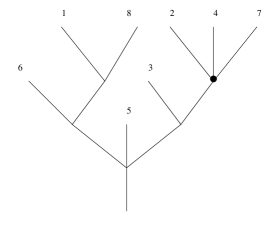
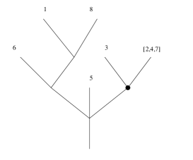
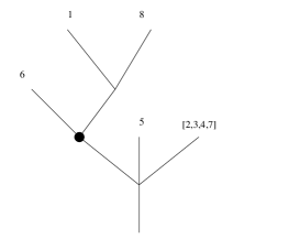
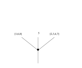
Figure 1. The pruning at node of a given tree. The bold internal node corresponds to the next chosen node.

1.2. Main result

The process $\Pi_{\text{GW}}^{[n]}$ is then a coalescent process starting from the trivial partition consisting of singletons and blocks merge together as time goes by. Its law is given in the next theorem.

Theorem 1.1.

We set $\alpha=\mathop{\frac{1}{\gamma}}\nolimits\in[1/2,1)$. The process $\Pi_{\text{GW}}^{[n]}$ is distributed under ${\mathbf{P}}_{n}$ as $\Pi^{[n]}_{\text{dis}}$ for the $\beta(1+\alpha,1-\alpha)$-coalescent with coalescent measure:

(4) $$\Lambda(dx)=\left(\frac{x}{1-x}\right)^{\alpha}\,dx.$$

Remark 1.2.

Notice that the process $\Pi^{[n]}_{\text{dis}}$ is discrete in time and thus characterizes the coalescent measure up to a multiplicative constant. It is possible to construct the continuous-time coalescent process $\Pi^{[n]}$ associated with the measure $\Lambda$ given by Equation (4) from the process $\Pi_{\text{GW}}^{[n]}$ by adding exponential times between the successive states of this process. More precisely, recall the definitions of the transitions rates $\lambda_{b,k}$ of Equation (1) and of the jump rates $\lambda_{b}$ of Equation (2). Let $(\tau_{k})_{k\in{\mathbb{N}}}$ be a sequence of independent random variables such that, conditionally given the process $\Pi_{\text{GW}}^{[n]}$, the random variable $\tau_{k}$ is exponentially distributed with parameter $\lambda_{\ell_{k}}$ where $\ell_{k}$ is the number of blocks of the partition $\Pi_{\text{GW}}^{[n]}(k)$, with the convention that $\tau_{k}=+\infty$ if $\ell_{k}=1$. Then we set

$$\tilde{\Pi}^{[n]}(t)=\Pi_{\text{GW}}^{[n]}(k)\quad\mbox{ if }\sum_{i=0}^{k-1}\tau_{i}\leq t<\sum_{i=0}^{k}\tau_{i}.$$

As a direct consequence of Theorem 1.1 and the definition of a $\Lambda$-coalescent, we get that the processes $\Pi^{[n]}$ and $\tilde{\Pi}^{[n]}$ have the same distribution.

One major drawback of this construction is that we define the process for fixed $n$ and not simultaneously for all $n$. However, as in [3], we can construct directly the process $(\Pi(\theta),\theta\geq 0)$ taking values in the set of partitions of the integers using the pruning of a Lévy continuum random tree. More precisely, we consider the weighted stable Lévy tree $({\mathcal{T}},d,\mathbf{m}^{\mathcal{T}})$ associated with the branching mechanism $\psi(\lambda)=\lambda^{\gamma}$ for $\gamma\in(1,2)$ (the case $\gamma=2$ is studied in [3] and requires a different pruning). We recall that ${\mathcal{T}}$ is a real tree and that $\mathbf{m}^{\mathcal{T}}$ corresponds to a uniform measure on the leaves of ${\mathcal{T}}$, see [21], [22] and also [9] more specifically for the space of weighted real trees. We work under the so-called normalized excursion measure ${\mathbb{N}}^{(1)}$ under which $\mathbf{m}^{\mathcal{T}}$ is a probability measure. We consider given ${\mathcal{T}}$ the pruning defined in [1]: to each branching point $x$ of ${\mathcal{T}}$ we can associate a “mass” $\Delta_{x}$ of this node, which intuitively represents the size of its progeny, and a random variable $E_{x}$ which is exponentially distributed with parameter $\Delta_{x}$. This random variable represents the time at which the node $x$ is cut. When we cut such a node, we remove the sub-tree above it. Let ${\mathcal{T}}_{\theta}$ denote the continuum random sub-tree obtained at time $\theta\geq 0$. We define a coalescent process using the usual paintbox procedure. Let $(U_{i},i\in{\mathbb{N}}^{*})$ be independent random variables with distribution $\mathbf{m}^{\mathcal{T}}$ under ${\mathbb{N}}^{(1)}$. We define a partition of ${\mathbb{N}}^{*}$ at time $\theta$, $\Pi_{\text{L\'{e}vy}}(\theta)$ by saying that two integers $i$ and $j$ belong to the same block of $\Pi_{\text{L\'{e}vy}}(\theta)$ if and only if the random variables $U_{i}$ and $U_{j}$ have a leaf of ${\mathcal{T}}_{\theta}$ as a common ancestor. Intuitively this means that $U_{i}$ and $U_{j}$ belong to the same sub-tree attached above ${\mathcal{T}}_{\theta}$. This defines a coalescent process $\Pi_{\text{L\'{e}vy}}=(\Pi_{\text{L\'{e}vy}}(\theta),\theta\geq 0)$. We are now interested in its discrete (in time) restriction to the $n$ first integers. Let $\Pi_{\text{L\'{e}vy}}^{[n]}=(\Pi_{\text{L\'{e}vy}}^{[n]}(k),k\in{\mathbb{N}})$ be the discrete process associated with $\Pi_{\text{L\'{e}vy}}$ restricted to the $n$ first integers until it reaches the absorbing state (which is the trivial partition consisting in one block) and which afterward remains constant.

By construction, and thanks to Theorem 3.2.1 in [21], we can deduce that under ${\mathbb{N}}^{(1)}$, the discrete coalescent process $\Pi_{\text{L\'{e}vy}}^{[n]}$ is distributed as $\Pi_{\text{GW}}^{[n]}$ under ${\mathbf{P}}_{n}$. In fact, we have the following stronger result.

Theorem 1.3.

We set $\alpha=\mathop{\frac{1}{\gamma}}\nolimits\in(1/2,1)$. Under ${\mathbb{N}}^{(1)}$, the processes $(\Pi_{\text{L\'{e}vy}}^{[n]},n\in{\mathbb{N}}^{*})$ associated with the Lévy tree with branching mechanism $\psi(\lambda)=\lambda^{\gamma}$ are distributed as $(\Pi_{\text{dis}}^{[n]},n\in{\mathbb{N}}^{*})$ associated with the Lévy measure $\Lambda(dx)=(x/1-x)^{\alpha}\,dx$.

Remark 1.4.

Although the process $\Pi_{\text{L\'{e}vy}}$ is a continuous-time process like $\Pi_{\text{GW}}$, it is not a coalescent process under ${\mathbb{N}}^{(1)}$ as for instance the time of the first coalescence event in $\Pi_{\text{L\'{e}vy}}^{[n]}$ is not exponentially distributed, see Corollary 4.5.

We conjecture that there exists a random time-change $(R(t),t\geq 0)$ such that the process $(\Pi_{\text{L\'{e}vy}}(R(t)),t\geq 0)$ is indeed under ${\mathbb{N}}^{(1)}$ a $\beta(1+\alpha,1-\alpha)$-coalescent, but we have no guess on what this time change could be.

Remark 1.5.

Let us remark that the $\beta(1+\alpha,1-\alpha)$-coalescent we obtain is also a $\beta(2-a,a)$-coalescent (with $a=1-\alpha$) as in [11] but with a different range for $a$. The difference between the two cases is that in [11] $\alpha\in(-1,0)$ and the coalescent process comes down from infinity (i.e. for every positive time $\theta$, the partition $\Pi(\theta)$ contains only a finite number of blocks) whereas in our case $\alpha\in(1/2,1)$ the process always contains an infinite number of singletons (also called “dust”).

Remark 1.6.

Let us remark that the pruning procedure described above is the same as in [36] used to construct the Miermont’s self-similar fragmentation process (see also [1]). However, the time reversal of the process $\Pi_{\text{L\'{e}vy}}$ is not Miermont’s fragmentation as once a sub-tree is cut and discarded, it is no more considered in our construction whereas it undergoes some others fragmentations in Miermont’s construction. There are still some strong connections. For instance, the tree ${\mathcal{T}}_{\theta}$ is linked with a tagged fragment in the fragmentation, see [1] Theorem 1.5 and Proposition 1.7 for the distribution of the tree ${\mathcal{T}}_{\theta}$ and for the distribution of a tagged fragment in Miermont’s fragmentation.

1.3. Number of cuts needed to isolate the root in a stable GW tree

Using the above link between Galton-Watson trees and $\beta$-coalescents, known results in one field translate immediately in the other field giving sometimes new results. In that direction, we first focus on how known asymptotics on the number of coalescence events yield new results on the number of cuts needed to isolate the root in a stable GW tree with $n$ leaves.

The original problem of cutting randomly a rooted tree arises first in Meir and Moon [35]. Given a rooted tree $T_{n}$ with $n$ edges, select an edge uniformly at random (notice that this is not exactly our pruning procedure) and delete the subtree not containing the root attached to this edge. On the remaining tree, iterate this procedure until only the edge attached to the root is left. We denote by $\tilde{Z}_{n}$ the number of edge-removals needed to isolate the root. The problem is then to study asymptotics of this random number $\tilde{Z}_{n}$, depending on the law of the initial tree $T_{n}$.

In the original paper [35], Meir and Moon considered Cayley trees and obtained asymptotics for the first two moments of $X_{n}$. Limits in distribution were then obtained, see for instance Panholzer [37] for some simply generated trees, Drmota, Iksanov, Möhle and Roesler [19] for random recursive trees, Holmgren [30] for binary search trees, Bertoin [13] for Cayley trees. In [31], Janson focuses on conditioned Galton-Watson trees associated with critical offspring distributions with finite variance and proves that

$$\tilde{Z}_{n}/\sqrt{n}\xrightarrow[n\rightarrow+\infty]{(d)}\;\tilde{Z},$$

where the random variable $\tilde{Z}$ has Rayleigh distribution with density $x\mathop{\mathrm{e}^{-x^{2}/2}}{\bf 1}_{\{x>0\}}$, and can be explicitly constructed using a pruning procedure on the Brownian continuum random tree (which corresponds to the cases $\gamma=2$ in our setting), see [5]. In particular $\tilde{Z}$ is distributed as the height of a random leaf of the Brownian continuum random tree. See also [10, 14] for further work on cutting randomly rooted trees.

Notice that the reproduction law for stable GW tree has an infinite variance for $\alpha\in(1/2,1)$, and the uniform pruning does not seem to be adapted to isolate the root. For this reason, we consider the pruning procedure developed in Section 1.1 to tackle the infinite variance case. So, let $Z_{n}$ be the number of cuts, using this procedure, needed to isolate the root of a stable GW tree:

$$Z_{n}=\inf\{k;\;\Pi^{[n]}_{\text{GW}}(k)=\{\{1,\ldots,n\}\}\}.$$

Notice that for $r$-ary trees, since all the internal nodes have the same degree the cutting procedure given in Section 1.1, corresponds to choose an internal node uniformly.

We immediately deduce from asymptotics of the number of coalescence events in $\beta$-coalescent (see Corollary 1 [28], see also [26], Table 1 for a summary of all the results concerning $\beta$-coalescents), the following result which extends part of the result in [31] to GW tree with infinite variance of the reproduction law.

Corollary 1.7.

Let $\alpha=1/\gamma\in[1/2,1)$. We have the following convergence in distribution:

$$n^{\alpha-1}Z_{n}\xrightarrow[n\rightarrow+\infty]{(d)}Z,$$

with the distribution of $Z$ characterized by, for $n\in{\mathbb{N}}^{*}$:

$${\mathbb{E}}\left[Z^{n}\right]=\alpha^{n}\frac{\Gamma(n+1)\Gamma(1-\alpha)}{\Gamma((n+1)(1-\alpha))}\cdot$$

Let us insist on the fact that this corollary does not need any proof as this is just a translation of known results on $\beta$-coalescents using our links with GW trees, only the moment computation needs some explanations and is done in Section 5,

The distribution of $Z$ corresponds to the expected limit distribution in the Conjecture that is stated at the end of the introduction in [4] for the number of cuts needed to isolate the root in general GW trees. (Notice that in the conjecture, one choose an internal node $x\in T$ with probability proportional to $k_{x}(T)$ whereas in Section 1.1 one choose an internal node $x\in T$ with probability proportional to $k_{x}(T)-1$.) In particular, $Z$ is distributed as the height of a random leaf of the normalized Lévy tree with branching mechanism $\psi(\lambda)=\lambda^{\gamma}$.

1.4. Number of blocks in the last coalescence event

On the other hand, we can use results on GW trees conditioned to have an infinite number of leaves (which is very close to Kesten’s result on GW tree conditionally on the non extinction, see [17] Theorem 3.1 or [6] Proposition 4.6) to get asymptotics on the number $B_{n}$ of blocks involved is the last coalescence event of $\Pi^{[n]}$.

The proof of the following Proposition is given in Section 6.

Proposition 1.8.

Let $\alpha=1/\gamma\in[1/2,1)$. We have the following convergence in distribution:

$$B_{n}\xrightarrow[n\rightarrow+\infty]{(d)}B,$$

with the distribution of $B$ given by its generating function $\varphi_{\alpha}(r)={\mathbb{E}}\left[r^{B}\right]$, with for $r\in[0,1]$:

(5) $$\varphi_{\alpha}(r)=(1-\alpha)r\int_{0}^{1}\frac{dx}{1-(1-x)^{\alpha}}\left(\mathop{\frac{1}{(1-rx)^{\alpha}}}\nolimits-1\right).$$

See also [3] for more results in this direction when $\alpha=1/2$ including the number of singletons involved in the last coalescence event as well as a closed form for $\varphi_{1/2}$.

Remark 1.9.

After we first posted this paper on arXiv, Hénard proved in [29] Theorem 3.5 that Equation (5) remains valid for all $\beta(1+\alpha,1-\alpha)$-coalescents with $\alpha\in(-1,1)$ (taking the limit when $\alpha=0$).

For $\alpha=0$, the $\beta(1+\alpha,1-\alpha)$-coalescent corresponds to the Bolthausen-Sznitman coalescent, and thus $\varphi_{0}$ is the generating function of the asymptotic number of blocks of the last coalescence event in the Bolthausen-Sznitman coalescent whose distribution is given in Theorem 3.1 and Proposition 3.2 of [27].

As $\alpha$ goes down to $-1$, we recover the Kingman’s coalescent as a limit. We also get $\varphi_{-1}(r)=r^{2}$ and notice that $\varphi_{-1}$ is trivially the generating function of the number of blocks of the last (in fact all) coalescence event in the Kingman’s coalescent, as all the coalescence events are binary.

1.5. Organization of the paper

Section 2 gives a representation of the pruning at node procedure for GW tree in continuous time motivated by [8]. This procedure corresponds in fact to the one presented in Introduction, Section 1.1. Section 3 is devoted to the proof of Theorem 1.1. Section 4 devoted to the proof of Theorem 1.3 is more technical as it relies on continuum random Lévy trees and the pruning of such trees as developed in [1]. Eventually Sections 5 and 6 are devoted to the proofs of Propositions 1.7 and 1.8.

2. Pruning at node of discrete GW trees

2.1. Discrete trees

Let us recall here the formalism for ordered discrete trees. We set

$${\mathcal{U}}=\bigcup_{n\geq 0}{({\mathbb{N}}^{*})^{n}}$$

the set of finite sequences of positive integers with the convention $({\mathbb{N}}^{*})^{0}=\{\emptyset\}$. For $u\in{\mathcal{U}}$ let $|u|$ be the length or generation of $u$ defined as the integer $n$ such that $u\in({\mathbb{N}}^{*})^{n}$. If $u$ and $v$ are two sequences of ${\mathcal{U}}$, we denote by $uv$ the concatenation of the two sequences, with the convention that $uv=u$ if $v=\emptyset$ and $uv=v$ if $u=\emptyset$. The set of ancestors of $u$ is the set:

(6) $$A_{u}=\{v\in{\mathcal{U}};\text{there exists $w\in{\mathcal{U}}$ such that $u=vw$}\}.$$

A discrete tree ${\mathbf{t}}$ is a subset of ${\mathcal{U}}$ that satisfies:

• $\emptyset\in{\mathbf{t}}$,

• If $u\in{\mathbf{t}}$, then $A_{u}\subset{\mathbf{t}}$.

• For every $u\in{\mathbf{t}}$, there exists a non-negative integer $k_{u}({\mathbf{t}})$ such that, for all positive integer $i$, $ui\in{\mathbf{t}}$ iff $1\leq i\leq k_{u}({\mathbf{t}})$.

The integer $k_{u}({\mathbf{t}})$ represents the number of offsprings of the node $u$ in the tree ${\mathbf{t}}$. We define ${\mathcal{L}}({\mathbf{t}})$ the set of leaves of ${\mathbf{t}}$ and ${\mathcal{N}}({\mathbf{t}})$ the set of internal nodes of ${\mathbf{t}}$ by:

$${\mathcal{L}}({\mathbf{t}})=\{u\in{\mathbf{t}},\ k_{u}({\mathbf{t}})=0\}\quad\text{and}\quad{\mathcal{N}}({\mathbf{t}})={\mathbf{t}}\setminus{\mathcal{L}}({\mathbf{t}}).$$

Let $L({\mathbf{t}})={\rm Card}\;({\mathcal{L}}({\mathbf{t}}))$ be the number of leaves of the tree ${\mathbf{t}}$, and notice that:

(7) $$L({\mathbf{t}})-1=\sum_{u\in{\mathcal{N}}({\mathbf{t}})}(k_{u}({\mathbf{t}})-1).$$

We denote by ${\mathbb{T}}$ the set of discrete trees and by ${\mathbb{T}}_{n}=\{{\mathbf{t}}\in{\mathbb{T}};L({\mathbf{t}})=n\}$ the set of discrete trees with $n$ leaves.

2.2. A discrete tree-valued process

We consider the pruning procedure developed in [7]. Let ${\mathbf{t}}\in{\mathbb{T}}$. Under some probability measure ${\mathbf{P}}^{\mathbf{t}}$, we consider a family of marks $(\xi_{u},u\in{\mathcal{U}})$ of independent non-negative real random variables (possibly infinite) such that:

• ${\mathbf{P}}^{\mathbf{t}}$-a.s. $\xi_{u}=+\infty$ if $u\not\in{\mathbf{t}}$ or if $u\in{\mathbf{t}}$ and $k_{u}({\mathbf{t}})\in\{0,1\}$,

• ${\mathbf{P}}^{\mathbf{t}}(\xi_{u}\geq\theta)=(1+\theta)^{1-k_{u}({\mathbf{t}})}$ if $u\in{\mathbf{t}}$ and $k_{u}({\mathbf{t}})\geq 2$.

At time $\theta$, we define the pruned tree ${\mathcal{P}}_{\theta}({\mathbf{t}})$ as the sub-tree given by:

$${\mathcal{P}}_{\theta}({\mathbf{t}})=\{u\in{\mathbf{t}};\,\xi_{v}>\theta\text{ for all }v\in A_{u},\,v\neq u\}.$$

In particular, we always have $\emptyset\in{\mathcal{P}}_{\theta}({\mathbf{t}})$.

For $u\in{\mathcal{N}}({\mathbf{t}})$, let $D_{u}$ be the event that $u$ is marked first, that is:

$$D_{u}=\{\xi_{u}=\min_{v\in{\mathcal{N}}({\mathbf{t}})}\xi_{v}\}.$$

Lemma 2.1.

We suppose that $L({\mathbf{t}})\neq 1$. Let $u\in{\mathcal{N}}({\mathbf{t}})$. We have:

$${\mathbf{P}}^{\mathbf{t}}(D_{u})=\frac{k_{u}({\mathbf{t}})-1}{L({\mathbf{t}})-1}\cdot$$

This lemma implies that the cutting procedure given in Section 1.1, corresponds to the successive states of the process $({\mathcal{P}}_{\theta}({\mathbf{t}}),\theta\geq 0)$.

Proof.

We have, using (7) for the last equality:

$${\mathbf{P}}^{\mathbf{t}}(D_{u}) ={\mathbf{P}}^{\mathbf{t}}(\xi_{u}\leq\xi_{v}\quad\forall v\neq u,v\in{\mathcal{N}}({\mathcal{T}}))$$

$$={\mathbf{E}}^{\mathbf{t}}\left[(1+\xi_{u})^{-\sum_{v\neq u,v\in{\mathcal{N}}({\mathbf{t}})}(k_{v}({\mathbf{t}})-1)}\right]$$

$$=(k_{u}({\mathbf{t}})-1)\int_{[0,+\infty)}(1+\theta)^{-\sum_{v\in{\mathcal{N}}({\mathbf{t}})}(k_{v}({\mathbf{t}})-1)-1}\;d\theta$$

$$=\frac{k_{u}({\mathbf{t}})-1}{\sum_{v\in{\mathcal{N}}({\mathbf{t}})}(k_{v}({\mathbf{t}})-1)}$$

$$=\frac{k_{u}({\mathbf{t}})-1}{L({\mathbf{t}})-1}\cdot$$

∎

2.3. Construction of the partition-valued process $\Pi_{\text{GW}}^{[n]}$

Let $\alpha\in[1/2,1)$. Recall that the function $g$ defined by (3) is the generating function of a probability measure $\nu_{g}$ on ${\mathbb{N}}$. We denote by $G_{g}(dT)$ the distribution on ${\mathbb{T}}$ of the critical GW tree with offspring distribution $\nu_{g}$. We will denote by ${\mathbf{P}}$ the probability measure on ${\mathbb{T}}\times[0,+\infty]^{\mathcal{U}}$:

$${\mathbf{P}}(dT,d\xi)=G_{g}(dT){\mathbf{P}}^{T}(d\xi).$$

Under ${\mathbf{P}}$, the random tree $T$ is a GW tree whose offspring distribution $\nu_{g}$ has generating function $g$ given by (3). According to Propositions 2.1 and 3.2 in [8], $({\mathcal{P}}_{\theta}(T),\theta\geq 0)$ is a Markov process and ${\mathcal{P}}_{\theta}(T)$ is a GW tree whose reproduction law has generating function $g_{\theta}$, with:

$$g_{\theta}(r)=1+(1+\theta)\left[g\left(\frac{r}{1+\theta}\right)-g\left(\mathop{\frac{1}{1+\theta}}\nolimits\right)\right].$$

Notice that:

(8) $$g_{\theta}(r)=r+\alpha\frac{(1-r+\theta)^{1/\alpha}-\theta^{1/\alpha}}{(1+\theta)^{(1/\alpha)-1}}\cdot$$

For every positive integer $n$, we set:

$${\mathbf{P}}_{n}(\bullet)={\mathbf{P}}(\bullet\bigm{|}L(T)=n).$$

Under ${\mathbf{P}}_{n}$, the distribution of the tree $T$ is given by the following formula (see [21], Theorem 3.3.3, or [34]), for ${\mathbf{t}}\in{\mathbb{T}}_{n}$:

(9) $${\mathbf{P}}_{n}(T={\mathbf{t}})=n!\left(\prod_{v\in{\mathcal{N}}({\mathbf{t}})}\frac{p_{k_{v}({\mathbf{t}})}}{k_{v}({\mathbf{t}})!}\right)\frac{\alpha^{n-1}\Gamma(1-\alpha)}{\Gamma(n-\alpha)}$$

where $p_{1}=0$ and, for $k\geq 2$, $p_{k}=\mathop{\left|(1-\gamma)(2-\gamma)\cdots(k-\gamma)\right|}\nolimits$.

Let $n\in{\mathbb{N}}^{*}$. Let $T$ be a random tree distributed as ${\mathbf{P}}_{n}$. Conditionally on $T$, we define a uniform random labeling $U_{1},\ldots,U_{n}$ of the leaves of $T$, independently of the variables $(\xi_{u},u\in T)$. Recall the set of ancestors defined in (6) and the pruning procedure ${\mathcal{P}}_{\theta}$ introduced in Section 2.2. We define the equivalence relation ${\mathcal{R}}_{\theta}^{[n]}$ on $\{1,2,\ldots,n\}$ by: $i{\mathcal{R}}_{\theta}^{[n]}j$ if $A_{U_{i}}\bigcap A_{U_{j}}\bigcap{\mathcal{L}}({\mathcal{P}}_{\theta}(T))$ is non empty, that is $U_{i}$ and $U_{j}$ have a leaf of ${\mathcal{P}}_{\theta}(T)$ as common ancestor. Then, for every $\theta\geq 0$, let $\hat{\Pi}_{\text{GW}}^{[n]}(\theta)$ be the equivalence classes of the equivalence relation ${\mathcal{R}}_{\theta}^{[n]}$ of the $n$ first integers. Let $\Pi_{\text{GW}}^{[n]}=(\Pi_{\text{GW}}^{[n]}(k),k\in{\mathbb{N}})$ be the discrete process associated with $\hat{\Pi}_{\text{GW}}^{[n]}=(\hat{\Pi}_{\text{GW}}^{[n]}(\theta),\theta\geq 0)$ until it reaches the absorbing state (which is the trivial partition consisting in one block) and afterward the discrete process remains constant.

We end this section with an elementary lemma which will be used in the proof of Theorem 1.1.

Lemma 2.2.

We have for $n\geq 2$:

(10) $${\mathbf{E}}_{n}\left[k_{\emptyset}(T)-1\right]=\frac{1-\alpha}{\alpha}\,\frac{\Gamma\left(1-\alpha\right)}{\Gamma\left(\alpha\right)}\,\frac{\Gamma\left(n-1+\alpha\right)}{\Gamma\left(n-\alpha\right)}\cdot$$

Proof.

We consider the generating function of $(k_{\emptyset}(T),L(T))$ under ${\mathbf{P}}$, that is $H(s,t)={\mathbf{E}}\left[s^{k_{\emptyset}(T)}t^{L(T)}\right]$. Using the branching property of GW trees, we have:

(11) $$H(s,t)={\mathbf{E}}\left[s^{k_{\emptyset}(T)}{\mathbf{E}}[t^{L(T)}]^{k_{\emptyset}(T)}{\bf 1}_{\{k_{\emptyset}(T)\neq 0\}}\right]+t{\mathbf{P}}(k_{\emptyset}(T)=0).$$

Notice that $g(s)={\mathbf{E}}\left[s^{k_{\emptyset}(T)}\right]=H(s,1)$. We set $h(t)=H(1,t)={\mathbf{E}}\left[t^{L(T)}\right]$ the generating function of $L(T)$. So that (11) becomes:

(12) $$H(s,t)=g(s\,h(t))-g(0)(1-t).$$

Taking $s=1$ in (12), we get:

(13) $$g(h(t))-h(t)=g(0)(1-t).$$

Using expression (3), we get:

$$h(t)=1-(1-t)^{\alpha}\quad\text{and}\quad H(s,t)=s\,h(t)+\alpha(1-s\,h(t))^{1/\alpha}-\alpha(1-t).$$

We deduce that:

$${\mathbf{E}}\left[k_{\emptyset}(T)t^{L(T)}\right]=\frac{\partial H}{\partial s}(1,t) =h(t)-h(t)(1-h(t))^{(1/\alpha)-1}$$

$$={\mathbf{E}}\left[t^{L(T)}\right]-\left[1-(1-t)^{\alpha}\right](1-t)^{1-\alpha}$$

$$={\mathbf{E}}\left[t^{L(T)}\right]-(1-t)^{1-\alpha}+1-t.$$

This gives:

$${\mathbf{E}}\left[(k_{\emptyset}(T)-1)t^{L(T)}\right]=-(1-t)^{1-\alpha}+1-t.$$

For $n\geq 2$, we get:

$${\mathbf{E}}\left[(k_{\emptyset}(T)-1){\bf 1}_{\{L(T)=n\}}\right] =\mathop{\frac{1}{n!}}\nolimits\left(\frac{d^{n}}{dt^{n}}{\mathbf{E}}\left[(k_{\emptyset}(T)-1)t^{L(T)}\right]\right)_{|_{t=0}}$$

$$=\mathop{\frac{1}{n!}}\nolimits\left(1-\alpha\right)\prod_{k=0}^{n-2}\left(\alpha+k\right)$$

$$=\mathop{\frac{1}{n!}}\nolimits\left(1-\alpha\right)\frac{\Gamma\left(n-1+\alpha\right)}{\Gamma\left(\alpha\right)}\cdot$$

We also get for $n\geq 2$:

$${\mathbf{P}}(L(T)=n)=\mathop{\frac{1}{n!}}\nolimits h^{(n)}(0)=\mathop{\frac{1}{n!}}\nolimits\alpha\prod_{k=1}^{n-1}\left(k-\alpha\right)=\mathop{\frac{1}{n!}}\nolimits\alpha\frac{\Gamma\left(n-\alpha\right)}{\Gamma\left(1-\alpha\right)}\cdot$$

We deduce that:

$${\mathbf{E}}_{n}\left[k_{\emptyset}(T)-1\right]=\frac{{\mathbf{E}}\left[(k_{\emptyset}(T)-1){\bf 1}_{\{L(T)=n\}}\right]}{{\mathbf{P}}(L(T)=n)}=\frac{1-\alpha}{\alpha}\frac{\Gamma(1-\alpha)}{\Gamma(\alpha)}\frac{\Gamma(n-1+\alpha)}{\Gamma(n-\alpha)}\cdot$$

∎

3. Proof of Theorem 1.1

Let $\alpha\in[1/2,1)$ and $\Lambda$ given by (4). Notice that the probability that the first coalescence event for $\Pi^{[n]}_{\text{dis}}$ corresponds to the collision of $k$ given blocks is $\lambda_{n,k}/\lambda_{n}$, with $\lambda_{n,k}$ and $\lambda_{n}$ given respectively by (1) and (2).

Theorem 1.1 is a direct consequence of Lemma 3.3 which states that the probability that the first coalescence event for $\Pi^{[n]}_{\text{GW}}$ corresponds to the collision of $k$ given blocks is $\lambda_{n,k}/\lambda_{n}$, and of Lemma 3.4, which states that after the first coalescence event, the law of the pruned tree under ${\mathbf{P}}_{n}$ conditionally given that it has $k$ leaves is exactly ${\mathbf{P}}_{k}$.

The proof of Lemme 3.3 (resp. 3.4) is given in Section 3.1 (resp. 3.2).

3.1. Computation of the coalescence rates

We first give an intermediate lemma. For $\alpha\in(0,1)$ and $\lambda>\alpha-1$, we set:

(14) $$\phi_{1+\alpha,1-\alpha}(\lambda)=\int_{0}^{1}\left(1-(1-x)^{\lambda}\right)x^{\alpha-2}(1-x)^{-\alpha}\;dx.$$

Lemma 3.1.

For $\alpha\in(0,1)$ and $\lambda>\alpha-1$, we have:

(15) $$\phi_{1+\alpha,1-\alpha}(\lambda)=\lambda\frac{\Gamma(\alpha)\Gamma(\lambda+1-\alpha)}{(1-\alpha)\Gamma(\lambda+1)}\cdot$$

Notice that for $\lambda>0$, (15) reduces to:

(16) $$\phi_{1+\alpha,1-\alpha}(\lambda)=\frac{\Gamma(\alpha)\Gamma(\lambda+1-\alpha)}{(1-\alpha)\Gamma(\lambda)}\cdot$$

Proof.

We set:

$$I=\int_{0}^{1}\left((1-u)^{-\alpha}-1\right)\;u^{\alpha-2}\,du.$$

Notice that $I$ is finite and $\phi_{1+\alpha,1-\alpha}(\alpha)=I$. For $\lambda>\alpha$, using an integration by part, we have:

$$\phi_{1+\alpha,1-\alpha}(\lambda) =\int_{0}^{1}\left(1-(1-x)^{\lambda}\right)x^{\alpha-2}(1-x)^{-\alpha}\;dx$$

$$=\int_{0}^{1}\left((1-x)^{-\alpha}-1\right)x^{\alpha-2}\;dx+\int_{0}^{1}\left(1-(1-x)^{\lambda-\alpha}\right)x^{\alpha-2}dx$$

$$=I-\mathop{\frac{1}{1-\alpha}}\nolimits+\frac{\lambda-\alpha}{1-\alpha}\int_{0}^{1}(1-x)^{\lambda-\alpha-1}x^{\alpha-1}\;dx$$

$$=I-\mathop{\frac{1}{1-\alpha}}\nolimits+\frac{\Gamma(\alpha)\Gamma(\lambda+1-\alpha)}{(1-\alpha)\Gamma(\lambda)}\cdot$$

We now compute $I$. For $\lambda=1$, we also have:

$$\phi_{1+\alpha,1-\alpha}(1)=\int_{0}^{1}x^{\alpha-1}(1-x)^{-\alpha}\;dx=\Gamma(\alpha)\Gamma(1-\alpha).$$

We deduce that:

$$I-\mathop{\frac{1}{1-\alpha}}\nolimits+\frac{\Gamma(\alpha)\Gamma(2-\alpha)}{(1-\alpha)\Gamma(1)}=\phi_{1+\alpha,1-\alpha}(1)=\Gamma(\alpha)\Gamma(1-\alpha).$$

This readily implies that $I=1/(1-\alpha)$ and thus (15) holds for $\lambda\geq\alpha$. Then uses that the right-hand sides of (14) and (15) are analytic for $\lambda>\alpha-1$ to get that (15) also holds for $\lambda>\alpha-1$. ∎

Recall that $\lambda_{n,k}$ and $\lambda_{n}$ are given respectively by (1) and (2), for $\Lambda$ given by (4).

Lemma 3.2.

Let $\alpha\in[1/2,1)$. We have for $2\leq k\leq n$:

(17) $$\frac{\lambda_{n,k}}{\lambda_{n}}=\frac{1-\alpha}{\Gamma(\alpha+1)}\frac{\Gamma(k+\alpha-1)\Gamma(n-k-\alpha+1)}{\Gamma(n-\alpha)}\frac{1}{n-1}\cdot$$

Proof.

We have

$$\lambda_{n,k} =\int_{0}^{1}u^{k-2}(1-u)^{n-k}\Lambda(du)$$

$$=\int_{0}^{1}u^{k-2+\alpha}(1-u)^{n-k-\alpha}du$$

$$=\beta(k+\alpha-1,n-k-\alpha+1)$$

$$=\frac{\Gamma(k+\alpha-1)\Gamma(n-k-\alpha+1)}{\Gamma(n)},$$

and

$$\lambda_{n}=\sum_{k=2}^{n}\left(\begin{array}[]{c}n\\ k\end{array}\right)\lambda_{n,k}=\int_{0}^{1}(1-(1-u)^{n}-nu(1-u)^{n-1})u^{-2}\Lambda(du).$$

Then using notations (14) and (16), we deduce that:

$$\lambda_{n} =\phi_{1+\alpha,1-\alpha}(n)-n\int_{0}^{1}u^{\alpha-1}(1-u)^{n-1-\alpha}\,du$$

$$=\frac{\Gamma(\alpha)\Gamma(n+1-\alpha)}{(1-\alpha)\Gamma(n)}-n\frac{\Gamma(\alpha)\Gamma(n-\alpha)}{\Gamma(n)}$$

$$=\left(\frac{n-\alpha}{1-\alpha}-n\right)\frac{\Gamma(\alpha)\Gamma(n-\alpha)}{\Gamma(n)}$$

$$=(n-1)\frac{\alpha}{1-\alpha}\frac{\Gamma(\alpha)\Gamma(n-\alpha)}{\Gamma(n)}\cdot$$

The expression obtained for $\lambda_{n,k}$ then gives the result. ∎

If ${\mathbf{t}}_{1}$ and ${\mathbf{t}}_{2}$ are two discrete trees and $u\in{\mathcal{L}}({\mathbf{t}}_{1})$ is a leaf of ${\mathbf{t}}_{1}$, we shall denote by ${\mathbf{t}}_{1}\circledast_{u}{\mathbf{t}}_{2}$ the tree obtained by grafting the tree ${\mathbf{t}}_{2}$ on the leaf $u$ of ${\mathbf{t}}_{1}$, that is:

(18) $${\mathbf{t}}_{1}\circledast_{u}{\mathbf{t}}_{2}={\mathbf{t}}_{1}\cup\{uv,\ v\in{\mathbf{t}}_{2}\}.$$

Lemma 3.3.

Let $\alpha\in[1/2,1)$. The probability under ${\mathbf{P}}_{n}$ that the first coalescence event in $\Pi_{\text{GW}}^{[n]}$ is the coalescence of $k$ given integers into one block is $\lambda_{n,k}/\lambda_{n}$.

Proof.

Let $A_{k}$ be the event that the first coalescence event corresponds to the $k$ first integers merging together. By exchangeability, the lemma is proved as soon as we check that ${\mathbf{P}}_{n}(A_{k})=\lambda_{n,k}/\lambda_{n}$.

The event $A_{k}$ is realized, if and only if:

• The initial tree $T$ is of the form ${\mathbf{t}}_{1}\circledast_{u}{\mathbf{t}}_{2}$ for some ${\mathbf{t}}_{2}\in{\mathbb{T}}_{k}$ and ${\mathbf{t}}_{1}\in{\mathbb{T}}_{n-k+1}$ and $u\in{\mathcal{L}}({\mathbf{t}}_{1})$.

• The leaves of ${\mathbf{t}}_{2}$ are labeled from $1$ to $k$ (and therefore, the leaves of ${\mathbf{t}}_{1}$ except $u$ are labeled from $k+1$ to $n$). This occurs with probability $\frac{k!(n-k)!}{n!}$.

• The first chosen node of ${\mathbf{t}}_{1}\circledast_{u}{\mathbf{t}}_{2}$ is $u$. This occurs according to Lemma 2.1 with probability $\frac{k_{\emptyset}({\mathbf{t}}_{2})-1}{n-1}$.

Thus, using (9) for the probability of having a given tree, we have:

$${\mathbf{P}}_{n}(A_{k}) =\sum_{\overset{{\mathbf{t}}_{1}\in{\mathbb{T}}_{n-k+1}}{\overset{{\mathbf{t}}_{2}\in{\mathbb{T}}_{k}}{u\in{\mathcal{L}}({\mathbf{t}}_{1})}}}{\mathbf{P}}_{n}(T={\mathbf{t}}_{1}\circledast_{u}{\mathbf{t}}_{2})\frac{k!(n-k)!}{n!}\frac{k_{\emptyset}({\mathbf{t}}_{2})-1}{n-1}$$

$$=\sum_{\overset{{\mathbf{t}}_{1}\in{\mathbb{T}}_{n-k+1}}{\overset{{\mathbf{t}}_{2}\in{\mathbb{T}}_{k}}{u\in{\mathcal{L}}({\mathbf{t}}_{1})}}}n!\left(\prod_{v\in{\mathcal{N}}({\mathbf{t}}_{1}\circledast_{u}{\mathbf{t}}_{2})}\frac{p_{k_{v}({\mathbf{t}}_{1}\circledast_{u}{\mathbf{t}}_{2})}}{k_{v}({\mathbf{t}}_{1}\circledast_{u}{\mathbf{t}}_{2})!}\right)\frac{\alpha^{n-1}\Gamma(1-\alpha)}{\Gamma(n-\alpha)}\frac{k!(n-k)!}{n!}\frac{k_{\emptyset}({\mathbf{t}}_{2})-1}{n-1}$$

$$=(n-k+1)\sum_{\overset{{\mathbf{t}}_{1}\in{\mathbb{T}}_{n-k+1}}{{\mathbf{t}}_{2}\in{\mathbb{T}}_{k}}}\frac{n!}{k!(n-k+1)!}{\mathbf{P}}_{n-k+1}(T={\mathbf{t}}_{1}){\mathbf{P}}_{k}(T={\mathbf{t}}_{2})$$

$$\qquad\qquad{\frac{\alpha^{n-1}\Gamma(1-\alpha)}{\Gamma(n-\alpha)}\frac{\Gamma(n-k-\alpha+1)}{\alpha^{n-k}\Gamma(1-\alpha)}\frac{\Gamma(k-\alpha)}{\alpha^{k-1}\Gamma(1-\alpha)}\frac{k!(n-k)!}{n!}\frac{k_{\emptyset}({\mathbf{t}}_{2})-1}{n-1}}$$

$$=\frac{\Gamma(n-k-\alpha+1)\Gamma(k-\alpha)}{\Gamma(n-\alpha)\Gamma(1-\alpha)}\frac{1}{n-1}{\mathbf{E}}_{k}\left[k_{\emptyset}(T)-1\right].$$

We then use Lemma 2.2 and Lemma 3.2 to conclude. ∎

3.2. Law of the tree after the first coalescence event

Let $S$ be the time of the first coalescence event and recall that ${\mathcal{P}}_{S}(T)$ denote the pruned tree at the first coalescence event.

Lemma 3.4.

Let ${\mathbf{t}}\in{\mathbb{T}}_{k}$. We have:

(19) $${\mathbf{P}}_{n}({\mathcal{P}}_{S}(T)={\mathbf{t}}\bigm{|}L({\mathcal{P}}_{S}(T))=k)={\mathbf{P}}_{k}(T={\mathbf{t}}).$$

Proof.

Let ${\mathbf{t}}\in{\mathbb{T}}_{k}$. We obtain ${\mathbf{t}}$ just after the first coalescence event if $T$ is of the form ${\mathbf{t}}\circledast_{u}{\mathbf{s}}$ for some $s\in{\mathbb{T}}_{n-k+1}$, $u\in{\mathcal{L}}({\mathbf{t}})$ and $u$ is the first chosen internal node. This gives:

$${\mathbf{P}}_{n}({\mathcal{P}}_{S}(T)={\mathbf{t}}) =\sum_{\overset{u\in{\mathcal{L}}({\mathbf{t}})}{{\mathbf{s}}\in{\mathbb{T}}_{n-k+1}}}{\mathbf{P}}_{n}(T={\mathbf{t}}\circledast_{u}{\mathbf{s}})\frac{k_{\emptyset}({\mathbf{s}})-1}{n-1}$$

$$=k\sum_{{\mathbf{s}}\in{\mathbb{T}}_{n-k+1}}n!\left(\prod_{v\in{\mathcal{N}}({\mathbf{t}})}\frac{p_{k_{v}({\mathbf{t}})}}{k_{v}({\mathbf{t}})!}\prod_{v\in{\mathcal{N}}({\mathbf{s}})}\frac{p_{k_{v}({\mathbf{s}})}}{k_{v}({\mathbf{s}})!}\right)\frac{\alpha^{n-1}\Gamma(1-\alpha)}{\Gamma(n-\alpha)}\frac{k_{\emptyset}({\mathbf{s}})-1}{n-1}$$

$$=k\sum_{{\mathbf{s}}\in{\mathbb{T}}_{n-k+1}}\frac{n!}{k!(n-k+1)!}{\mathbf{P}}_{k}(T={\mathbf{t}}){\mathbf{P}}_{n-k+1}(T={\mathbf{s}})$$

$$\qquad\qquad\frac{\alpha^{n-1}\Gamma(1-\alpha)}{\Gamma(n-\alpha)}\frac{\Gamma(k-\alpha)}{\alpha^{k-1}\Gamma(1-\alpha)}\frac{\Gamma(n-k+1-\alpha)}{\alpha^{n-k}\Gamma(1-\alpha)}\frac{k_{\emptyset}({\mathbf{s}})-1}{n-1}$$

$$=\frac{n!}{(k-1)!(n-k+1)!}\frac{\Gamma(n-k+1-\alpha)\Gamma(k-\alpha)}{\Gamma(n-\alpha)\Gamma(1-\alpha)}$$

$$\qquad\qquad\qquad\qquad\mathop{\frac{1}{n-1}}\nolimits{\mathbf{E}}_{n-k+1}[k_{\emptyset}(T)-1]{\mathbf{P}}_{k}(T={\mathbf{t}}).$$

As the term in front of ${\mathbf{P}}_{k}(T={\mathbf{t}})$ does not depend on ${\mathbf{t}}$, it has to be equal to ${\mathbf{P}}_{n}(L({\mathcal{P}}_{S}(T))=k)$ and therefore (19) holds. ∎

4. Pruning of rooted real trees and proof of Theorem 1.3

The aim of this section is to use the pruning procedure for Lévy trees developed in [1] to give a consistent representation of the family of coalescent processes $(\hat{\Pi}^{[n]}_{\text{GW}},n\in{\mathbb{N}}^{*})$, see Corollary 4.4 and thus deduce Theorem 1.3.

4.1. The CRT framework

4.1.1. Real trees

Real trees have been introduced first in the field of geometric group theory (see for instance [18]) and then used later for defining continuum random trees (the framework first appeared in [23]). A real tree is a metric space $({\mathcal{T}},d)$ satisfying the following two properties for every $x,y\in{\mathcal{T}}$:

• (unique geodesic) There is a unique isometric map $f_{x,y}$ from $[0,d(x,y)]$ into ${\mathcal{T}}$ such that $f_{x,y}(0)=x$ and $f_{x,y}(d(x,y))=y$.

• (no loop) If $\varphi$ is a continuous injective map from $[0,1]$ into ${\mathcal{T}}$ such that $\varphi(0)=x$ and $\varphi(1)=y$, then

  $$\varphi([0,1])=f_{x,y}([0,d(x,y)]).$$

A rooted real tree is a real tree with a distinguished vertex denoted $\emptyset$ and called the root.

For every $x,y\in{\mathcal{T}}$, we denote by $[\![x,y]\!]$ the range of the map $f_{x,y}$ (i.e. the only path in the tree that links $x$ to $y$) and we set $[\![x,y[\![=[\![x,y]\!]\setminus\{y\}$.

If ${\mathcal{T}}$ is a rooted real tree, for $x\in{\mathcal{T}}$, we define the degree of $x$, denoted by $n_{x}$, as the number of connected components of ${\mathcal{T}}\setminus\{x\}$. The leaves of ${\mathcal{T}}$ is ${\mathcal{L}}({\mathcal{T}})=\{x\in{\mathcal{T}}\setminus\{\emptyset\};\,n_{x}=1\}$. If $n_{x}\geq 3$, we say that $x$ is a branching point of ${\mathcal{T}}$. We denote by ${\mathcal{B}}_{\text{br}}({\mathcal{T}})$ the set of branching points of ${\mathcal{T}}$. The height of ${\mathcal{T}}$ is $H_{\text{max}}({\mathcal{T}})=\sup\{d(\emptyset,x);\;x\in{\mathcal{T}}\}$. Let $(x_{i},i\in I)$ be a family of elements of ${\mathcal{T}}$, we define their most recent common ancestor denoted by $\text{MRCA}(x_{i},i\in I)$ as the element $x$ of ${\mathcal{T}}$ such that $[\![\emptyset,x]\!]=\bigcap_{i\in I}[\![\emptyset,x_{i}]\!]$.

A weighted rooted real tree $({\mathcal{T}},d,\mathbf{m})$ is a rooted real tree $({\mathcal{T}},d)$ endowed with a $\sigma$-finite measure $\mathbf{m}$ called the mass measure.

4.1.2. Stable Lévy tree

Set $\psi(\lambda)=\lambda^{\gamma}$ with $\gamma\in(1,2)$. We refer to [22] and [9] for the existence of a measure ${\mathbb{N}}[d{\mathcal{T}}]$ on the set of weighted locally compact rooted real tree such that ${\mathcal{T}}$ is under ${\mathbb{N}}[d{\mathcal{T}}]$ a Lévy tree associated with the branching mechanism $\psi$. For the Lévy tree $({\mathcal{T}},d,\mathbf{m})$, ${\mathbb{N}}[d{\mathcal{T}}]$ -a.e., the mass measure has support ${\mathcal{L}}({\mathcal{T}})$ and has no atom. Furthermore, ${\mathbb{N}}[d{\mathcal{T}}]$-a.e., all the branching points of the tree are of infinite degree. Following [22], there exists a local time process $(\ell^{a},a\geq 0)$ with values on finite measures on ${\mathcal{T}}$, which is càdlàg for the weak topology on finite measures on ${\mathcal{T}}$ and such that ${\mathbb{N}}^{\psi}[d{\mathcal{T}}]$-a.e.:

$$\mathbf{m}(dx)=\int_{0}^{\infty}\ell^{a}(dx)\,da,$$

$\ell^{0}=0$, $\inf\{a>0;\ell^{a}=0\}=\sup\{a\geq 0;\ell^{a}\neq 0\}=H_{\text{max}}({\mathcal{T}})$ and for every fixed $a\geq 0$, ${\mathbb{N}}^{\psi}[d{\mathcal{T}}]$-a.e. the measure $\ell^{a}$ is supported on $\{x\in{\mathcal{T}};d(\emptyset,x)=a\}$ and the real valued process $(\langle\ell^{a},1\rangle,a\geq 0)$ is distributed as a continuous state branching process (CSBP) with branching mechanism $\psi$ under its canonical measure. In particular, as the total size of a critical CSBP is finite, we get that ${\mathbb{N}}$-a.e. $\sigma=\mathbf{m}({\mathcal{T}})$ is finite.

The set $\{d(\emptyset,x),\ x\in\mathrm{Br}({\mathcal{T}})\}$ coincides ${\mathbb{N}}^{\psi}$-a.e. with the set of discontinuity times of the mapping $a\mapsto\ell^{a}$. Moreover, ${\mathbb{N}}^{\psi}$-a.e., for every such discontinuity time $b$, there is a unique $x\in{\mathcal{B}}_{\text{br}}({\mathcal{T}})$ such that $d(\emptyset,x)=b$ and $\Delta_{x}>0$, such that:

$$\ell^{b}=\ell^{b-}+\Delta_{x}\delta_{x},$$

where $\Delta_{x}>0$ is called the mass of the node $x$. Intuitively $\Delta_{x}$ represents the size of the progeny of $x$.

The scaling property of the stable Lévy tree implies that there exists a well defined probability measure ${\mathbb{N}}^{(1)}$ defined as the measure ${\mathbb{N}}$ conditioned on $\{\sigma=1\}$. The probability measure is also referred as the normalized excursion measure for Lévy trees.

4.2. The partition-valued process

Set $\psi(\lambda)=\lambda^{\gamma}$ with $\gamma\in(1,2)$.

4.2.1. Pruning of the stable Lévy tree

We consider the pruning procedure introduced in [1] (this procedure is defined when there is no Brownian part in the Lévy process with index given by the branching mechanism $\psi$). Under ${\mathbb{N}}$ or ${\mathbb{N}}^{(1)}$, conditionally given ${\mathcal{T}}$, we consider a family $(E_{x},x\in{\mathcal{B}}_{\text{br}}({\mathcal{T}}))$ of independent real random variables such that the random variable $E_{x}$ is exponentially distributed with parameter $\Delta_{x}$. This random variable represents the time at which the branching point $x$ is marked. For every $\theta>0$, we set

$${\mathcal{T}}_{\theta}=\{x\in{\mathcal{T}},\ \forall y\in[\![\emptyset,x[\![,\ E_{y}\geq\theta\}.$$

The set ${\mathcal{T}}_{\theta}$ is still a real tree which represents the tree ${\mathcal{T}}$ pruned at time $\theta$: we cut ${\mathcal{T}}$ at the points that are marked before time $\theta$ and keep the connected component of the tree that contains the root. We set ${\mathcal{T}}_{0}={\mathcal{T}}$. By [1], Theorem 1.5, the tree ${\mathcal{T}}_{\theta}$ is distributed under ${\mathbb{N}}$ as a Lévy tree with branching mechanism $\psi_{\theta}$ defined by:

$$\psi_{\theta}(\lambda)=\psi(\lambda+\theta)-\psi(\theta).$$

Moreover, by [2], the process $({\mathcal{T}}_{\theta},\theta\geq 0)$ is under ${\mathbb{N}}$ a Markov process.

4.2.2. Definition of the partition-valued process

Under ${\mathbb{N}}$ or ${\mathbb{N}}^{(1)}$, conditionally on ${\mathcal{T}}$, let $(F_{i},i\in{\mathbb{N}}^{*})$ be independent random variables on ${\mathcal{T}}$ distributed according to the probability mass measure $\mathbf{m}/\mathbf{m}({\mathcal{T}})$, and independent of the marks $(E_{x},x\in{\mathcal{B}}_{\text{br}}({\mathcal{T}}))$. Notice that ${\mathbb{N}}$-a.e. or ${\mathbb{N}}^{(1)}$-a.s. $(F_{i},i\in{\mathbb{N}}^{*})$ are leaves of ${\mathcal{T}}$. For $\theta\geq 0$, we define the equivalence relation ${\mathcal{R}}_{\theta}^{\text{L\'{e}vy}}$ on ${\mathbb{N}}^{*}$ by: $i{\mathcal{R}}_{\theta}^{\text{L\'{e}vy}}j$ if $[\![\emptyset,F_{i}]\!]\bigcap[\![\emptyset,F_{j}]\!]\bigcap{\mathcal{L}}({\mathcal{T}}_{\theta})$ is non empty, that is $F_{i}$ and $F_{j}$ have a leaf of ${\mathcal{T}}_{\theta}$ as common ancestor. This is very close to the definition of the equivalence relation ${\mathcal{R}}_{\theta}^{\text{[n]}}$ defined in Section 2.3. We denote by $\Pi_{\text{L\'{e}vy}}(\theta)$ the partition of ${\mathbb{N}}^{*}$ formed by the equivalence classes of ${\mathcal{R}}_{\theta}^{\text{L\'{e}vy}}$ and set $\Pi_{\text{L\'{e}vy}}=(\Pi_{\text{L\'{e}vy}}(\theta),\theta\geq 0)$.

4.3. Lévy sub-trees

4.3.1. Skeleton of finite real tree

Let $\hat{\mathbf{t}}$ be a real tree with finite height and a finite number of leaves, such that the leaves $(f_{i},i\in I(\hat{\mathbf{t}}))$ are indexed by a totally ordered set $I(\hat{\mathbf{t}})$. We define the skeleton $\tilde{\mathbf{t}}$ of the tree $\hat{\mathbf{t}}$ as the discrete tree (belonging to ${\mathbb{T}}$) where we forget the edge lengths. As the trees in ${\mathbb{T}}$ are ordered, we must be a bit more rigorous for the definition of $\tilde{\mathbf{t}}$.

The skeleton $\tilde{\mathbf{t}}$ of the real tree with ordered leaves $\left(\hat{\mathbf{t}},(f_{i},i\in I(\hat{\mathbf{t}}))\right)$ is defined recursively as follows. We define $k_{\emptyset}(\tilde{\mathbf{t}})$ as the degree of $\text{MRCA}(f_{i},i\in I(\hat{\mathbf{t}}))$ the ancestor of all the leaves of $\hat{\mathbf{t}}$. If $k_{\emptyset}(\tilde{\mathbf{t}})=0$, then $\tilde{\mathbf{t}}$ is reduced to $\emptyset$. In this case $\hat{\mathbf{t}}$ has one leaf, let $f$ be its label, and the discrete tree $\tilde{\mathbf{t}}$ has thus one leaf to which we give the label $f$. If $k_{\emptyset}(\tilde{\mathbf{t}})>0$, then we consider the $k_{\emptyset}(\tilde{\mathbf{t}})$ connected components of $\hat{\mathbf{t}}\setminus\{\text{MRCA}(f_{i},i\in I(\hat{\mathbf{t}}))\}$ that do not contain the root and label them from 1 to $k_{\emptyset}(\tilde{\mathbf{t}})$ according to the lowest label of the leaves of $\hat{\mathbf{t}}$ which belongs to them. This gives an ordered family $(\hat{\mathbf{t}}_{k},k\in\{1,\ldots,k_{\emptyset}(\tilde{\mathbf{t}})\})$ of real trees, and let $\text{MRCA}(f_{i},i\in I(\hat{\mathbf{t}}))\})$ be the root of each one. For $k\in\{1,\ldots,k_{\emptyset}(\tilde{\mathbf{t}})\}$, let $I(\hat{\mathbf{t}}_{k})=\{i\in I(\hat{\mathbf{t}});f_{i}\in\hat{\mathbf{t}}_{k})$ be the labels of the leaves of $\hat{\mathbf{t}}_{k}$ and the discrete tree $\tilde{\mathbf{t}}_{k}$ is the skeleton of $\left(\hat{\mathbf{t}}_{k},(f_{i},i\in I(\hat{\mathbf{t}}_{k}))\right)$.

Notice that $\tilde{\mathbf{t}}$ is finite, $k_{u}(\tilde{\mathbf{t}})\neq 1$ for all $u\in\tilde{\mathbf{t}}$, and $\hat{\mathbf{t}}$ and $\tilde{\mathbf{t}}$ have the same number of leaves. In the previous construction to a leaf $f_{i}$ of $\hat{\mathbf{t}}$ with label $i$ corresponds a unique leaf $e_{i}$ of $\tilde{\mathbf{t}}$ with label $i$. For $u\in\tilde{\mathbf{t}}$, we define $\tilde{\mathbf{t}}_{u}$ the sub-tree of $\tilde{\mathbf{t}}$ attached to the node $u$ i.e.

(20) $$\tilde{\mathbf{t}}_{u}=\{w\in{\mathcal{U}},\ uw\in\tilde{\mathbf{t}}\},$$

and let $I_{u}=\{i;e_{i}\in\tilde{\mathbf{t}}_{u}\}$. Define $\hat{\mathbf{t}}_{u}$ as ${\mathbf{s}}_{u}=\hat{\mathbf{t}}\backslash\bigcup_{i\not\in I_{u}}[\![\emptyset,f_{i}]\!]$ to which we add the root $\emptyset_{u}=\overline{{\mathbf{s}}_{u}}\backslash{\mathbf{s}}_{u}$, and $I(\hat{\mathbf{t}}_{u})=\{i;e_{i}\in\tilde{\mathbf{t}}_{u}\}$. Notice that by construction $\tilde{\mathbf{t}}_{u}$ is the skeleton of $\left(\hat{\mathbf{t}}_{u},(f_{i};i\in I(\hat{\mathbf{t}}_{u}))\right)$. We say that $u\in\tilde{\mathbf{t}}$ are the individuals of $\hat{\mathbf{t}}$, and define their lifetime as the length $h_{u}$ of the geodesic $B(u)=[\![\emptyset_{u},\text{MRCA}(f_{i},i\in I(\hat{\mathbf{t}}_{u}))]\!]$. We say the corresponding node in $\hat{\mathbf{t}}$ of $u\in\tilde{\mathbf{t}}$ is $C(u)=\text{MRCA}(f_{i},i\in I(\hat{\mathbf{t}}_{u}))$.

Notice it is easy to reconstruct $\hat{\mathbf{t}}$ from $\tilde{\mathbf{t}}$ and the family of lifetime $(h_{u},u\in\tilde{\mathbf{t}})$.

4.3.2. Coalescence of Lévy tree and GW tree

Let $M$ be, under ${\mathbb{N}}$ or ${\mathbb{N}}^{(1)}$ conditionally on ${\mathcal{T}}$, a Poisson random variable with finite mean $\sigma=\mathbf{m}({\mathcal{T}})$. We shall work on $\{M\geq 1\}$. On $\{M\geq 1\}$, let $\hat{T}_{0}$ be the real sub-tree of ${\mathcal{T}}$ generated by the root and $(F_{i},1\leq i\leq M)$:

$$\hat{T}_{0}=\bigcup_{1\leq i\leq M}[\![\emptyset,F_{i}]\!].$$

Since $\mathbf{m}$ has support ${\mathcal{L}}({\mathcal{T}})$ and has no atom, we deduce that $(F_{i},1\leq i\leq M)$ are distinct and are the leaves of $\hat{T}_{0}$.

We denote by $\tilde{T}_{0}$ the skeleton of $\hat{T}_{0}$ with the labeled leaves $(F_{i},1\leq i\leq M)$. According to [21], Theorem 3.2.1, the tree $\hat{T}_{0}$ is distributed under ${\mathbb{N}}[\;\cdot\bigm{|}M\geq 1]$ as a continuous GW tree (i.e. a GW tree with edge-lengths) such that

• The discrete tree $\tilde{T}_{0}$ is a GW tree with offspring distribution characterized by its generating function $g$ defined by (3) with $\alpha=1/\gamma$.

• Lifetimes of individuals $(h_{u},u\in\tilde{T}_{0})$ are independent random variables with exponential distribution with parameter $\gamma$.

We must first prove the following lemma which will be a key point in the sequel. Its proof relies on the scaling property of the Lévy tree.

Lemma 4.1.

The distributions of $\hat{T}_{0}$ under ${\mathbb{N}}[\;\cdot\bigm{|}M=n]$ and under ${\mathbb{N}}^{(1)}[\;\cdot\bigm{|}M=n]$ are the same.

Proof.

For a tree ${\mathcal{T}}$ and points $x_{1},\ldots,x_{n}$ of ${\mathcal{T}}$, let us denote by $T({\mathcal{T}},x_{1},\ldots,x_{n})$ the tree spanned by the points $(x_{i})$ and the root of the tree and $\tilde{T}({\mathcal{T}},x_{1},\ldots,x_{n})$ the associated discrete tree so that under ${\mathbb{N}}[\;\cdot\bigm{|}M=n]$ or ${\mathbb{N}}^{(1)}[\;\cdot\bigm{|}M=n]$, we have

$$\tilde{T}_{0}=\tilde{T}({\mathcal{T}},F_{1},\ldots,F_{n}).$$

Then, for every bounded measurable function $\phi$, we have

$${\mathbb{N}}\left[\phi\bigl{(}\tilde{T}({\mathcal{T}},F_{1},\ldots,F_{n})\bigr{)}{\bf 1}_{\{M=n\}}\right]={\mathbb{N}}\left[\phi\bigl{(}\tilde{T}({\mathcal{T}},F_{1},\ldots,F_{n})\bigr{)}\frac{\sigma^{n}}{n!}\mathop{\mathrm{e}^{-\sigma}}\right].$$

Let $\nu$ be the distribution of $\sigma$ under ${\mathbb{N}}$ i.e. the only measure $\nu$ such that for every $\lambda>0$,

$$\int_{0}^{+\infty}(1-\mathop{\mathrm{e}^{-\lambda u}})\nu(du)=\lambda^{\alpha}.$$

Then we have

$${\mathbb{N}}\left[\phi\bigl{(}\tilde{T}({\mathcal{T}},F_{1},\ldots,F_{n})\bigr{)}{\bf 1}_{\{M=n\}}\right]=\int_{0}^{+\infty}{\mathbb{N}}^{(u)}\left[\phi\bigl{(}\tilde{T}({\mathcal{T}},F_{1},\ldots,F_{n})\bigr{)}\right]\frac{u^{n}}{n!}\mathop{\mathrm{e}^{-u}}\nu(du).$$

Using the scaling property of the stable Lévy tree (see [21] Section 3.3), we have that the law of the tree ${\mathcal{T}}$ under ${\mathbb{N}}^{(u)}$ is the same as the law of $u^{1-\alpha}{\mathcal{T}}$ under ${\mathbb{N}}^{(1)}$ where the notation $\lambda{\mathcal{T}}$ means that we multiply the distance that defines ${\mathcal{T}}$ by the factor $\lambda$ (i.e. we scale all the edge lengths by $\lambda$). Moreover, as we only look at discrete trees, this factor does not modify the tree $\tilde{T}_{0}$. Therefore, we get:

$${\mathbb{N}}\left[\phi\bigl{(}\tilde{T}({\mathcal{T}},F_{1},\ldots,F_{n})\bigr{)}{\bf 1}_{\{M=n\}}\right] =\int_{0}^{+\infty}{\mathbb{N}}^{(1)}\left[\phi\bigl{(}\tilde{T}({\mathcal{T}},F_{1},\ldots,F_{n})\bigr{)}\right]\frac{u^{n}}{n!}\mathop{\mathrm{e}^{-u}}\nu(du)$$

$$={\mathbb{N}}^{(1)}\left[\phi\bigl{(}\tilde{T}({\mathcal{T}},F_{1},\ldots,F_{n})\bigr{)}\right]{\mathbb{N}}[M=n].$$

We deduce:

$${\mathbb{N}}[\phi(\tilde{T}_{0})\bigm{|}M=n]={\mathbb{N}}\left[\phi\bigl{(}\tilde{T}({\mathcal{T}},F_{1},\ldots,F_{n})\bigr{)}\bigm{|}M=n\right]\\ ={\mathbb{N}}^{(1)}\left[\phi\bigl{(}\tilde{T}({\mathcal{T}},F_{1},\ldots,F_{n})\bigr{)}\right]={\mathbb{N}}^{(1)}[\phi(\tilde{T}_{0})\bigm{|}M=n]$$

since ${\mathcal{T}}$ and $M$ are independent under ${\mathbb{N}}^{(1)}$. ∎

We now consider the marks that define the pruned tree ${\mathcal{T}}_{\theta}$ and we define on the event $\{M\geq 1\}$ the tree $\hat{T}_{\theta}$ as the tree $\hat{T}_{0}$ pruned on the same marks, in other words, we set

$$\hat{T}_{\theta}=\hat{T}_{0}\cap{\mathcal{T}}_{\theta}.$$

Let $\hat{\Pi}_{\text{L\'{e}vy}}^{[n]}$ be the restriction of $\Pi_{\text{L\'{e}vy}}$ to the $n$ first integers. By construction, if $C_{\theta}$ is an element of $\hat{\Pi}_{\text{L\'{e}vy}}^{[n]}(\theta)$, then there exists a leaf $x$ of $\hat{T}_{\theta}$ such that $x$ belongs to the sub-tree $\bigcup_{i\in C_{\theta}}[\![\emptyset,F_{i}]\!]$, and $x$ is the only leaf of $\hat{T}_{\theta}$ with this property. We set $C_{\theta}$ for the label of $x$, and we consider the order of the elements of $\tilde{\Pi}_{\text{L\'{e}vy}}^{[n]}$ given by the order of their smallest integer. We set $I_{\theta}=I(\hat{T}_{\theta})$ for the labels of the leaves of $\hat{T}_{\theta}$ and $(F^{\theta}_{i},i\in I_{\theta})$ for the leaves of $\hat{T}_{\theta}$.

We denote by $\tilde{T}_{\theta}$ the skeleton of $\hat{T}_{\theta}$ with the labeled leaves $(F_{i}^{\theta},i\in I_{\theta})$. According to [8], Proposition 4.1, the tree $\hat{T}_{\theta}$ is distributed under ${\mathbb{N}}[\;\cdot\bigm{|}M\geq 1]$ as a continuous GW tree such that

• $\tilde{T}_{\theta}$ is a GW tree with offspring distribution characterized by its generating function $g_{\theta}$ given in (8) with $\alpha=1/\gamma$.

• The lifetimes of individuals $(h_{u},u\in\hat{T}_{\theta})$ are independent random variable with exponential distribution with parameter $\psi_{\theta}^{\prime}(1)=\gamma(1+\theta)^{\gamma-1}$.

The following Lemma is a consequence of Theorem 6.1 of [8].

Lemma 4.2.

The process $(\tilde{T}_{\theta},\theta\geq 0)$ is distributed under ${\mathbb{N}}[\;\cdot\bigm{|}M\geq 1]$ as the process $({\mathcal{P}}_{\theta}(T),\theta\geq 0)$ under ${\mathbf{P}}$.

Proof.

Let $\theta>0$. Theorem 6.1 of [8] describes how $\hat{T}_{\theta}$ is obtained from $\hat{T}_{0}$:

• A branching point $x$ of $\hat{T}_{0}$ with $k_{x}=k_{x}(\hat{T}_{0})$ children is marked at time $\tau_{x}$ with distribution given by:

  $${\mathbb{N}}[\tau_{x}\geq\theta\bigm{|}\hat{T}_{0}]=-\int_{\theta}^{+\infty}\frac{\psi^{(k_{x}+1)}(1+z)}{\psi^{(k_{x})}(1)}dz=\frac{\psi^{(k_{x})}(1+\theta)}{\psi^{(k_{x})}(1)}=\left(\frac{1}{1+\theta}\right)^{k_{x}-\gamma}.$$

• A branch $B$ of length $h$ is marked at time $\tau_{B}$ with distribution given by:

  $${\mathbb{N}}[\tau_{B}\geq\theta\bigm{|}\hat{T}_{0}]=\exp\left(-h\int_{0}^{\theta}\psi^{\prime\prime}(1+z)dz\right)=\mathop{\mathrm{e}^{-\bigl{(}\psi^{\prime}(1+\theta)-\psi^{\prime}(1)\bigr{)}h}}.$$

Then the tree $\hat{T}_{0}$ is cut according to the marks present at time $\theta$ and the tree $\hat{T}_{\theta}$ is the connected component that contains the root. Therefore, the tree $\tilde{T}_{\theta}$ is obtained from the tree $\tilde{T}_{0}$ by a pruning at node. A node $u\in\tilde{T}_{0}$ is marked if the corresponding node $C(u)\in\hat{T}_{0}$ is marked at time $\theta$ in the previous procedure OR the branch $B(u)$ with length $h_{u}$ is marked. So the node $u$ of $\tilde{T}_{0}$ is marked at time $\zeta_{u}=\tau_{C(u)}\wedge\tau_{B(u)}$ and using that the edge lengths of $\hat{T}_{0}$ are independent and exponentially distributed with parameter $\gamma=\psi^{\prime}(1)$, we have with $k_{u}=k_{u}(\hat{T}_{0})$:

$${\mathbb{N}}[\zeta_{u}\geq\theta\bigm{|}\tilde{T}_{0}] ={\mathbb{N}}[\tau_{C(u)}\geq\theta\bigm{|}\tilde{T}_{0}]\;{\mathbb{N}}[\tau_{B(u)}\geq\theta\bigm{|}\tilde{T}_{0}]$$

$$=\left(\mathop{\frac{1}{1+\theta}}\nolimits\right)^{k_{u}-\gamma}\int_{0}^{+\infty}dh\,\gamma\mathop{\mathrm{e}^{-\gamma h}}\mathop{\mathrm{e}^{-\bigl{(}\psi^{\prime}(1+\theta)-\gamma\bigr{)}h}}$$

$$=\left(\mathop{\frac{1}{1+\theta}}\nolimits\right)^{k_{u}-\gamma}\left(\mathop{\frac{1}{1+\theta}}\nolimits\right)^{\gamma-1}$$

$$=\left(\frac{1}{1+\theta}\right)^{k_{u}-1}\cdot$$

Since the cutting time $\tau_{C(u)}$ and $\tau_{B(u)}$ are independent for all internal nodes $u$, we recover the discrete pruning procedure that defines the process $({\mathcal{P}}_{\theta}(T),\theta\geq 0)$ under ${\mathbf{P}}$. To conclude notice that $\tilde{T}_{0}$ and $T$ are GW tree with offspring distribution characterized by its generating function $g$. ∎

4.4. Proof of Theorem 1.3

The next corollary states that the pruning procedure for stable GW tree developed in [7] and the pruning procedure for Lévy trees developed in [1] and applied in [8] to sub-trees with finite number of leaves coincide.

Corollary 4.3.

Let $n\in{\mathbb{N}}$. The process $(\tilde{T}_{\theta},\theta\geq 0)$ is distributed under ${\mathbb{N}}[\;\cdot\bigm{|}M=n]$ as the process $({\mathcal{P}}_{\theta}(T),\theta\geq 0)$ under ${\mathbf{P}}_{n}$.

Proof.

This is a direct consequence of Lemma 4.2 and the fact that $M=L(\tilde{T}_{0})$. ∎

Theorem 1.3 follows directly from Theorem 1.1 and from the following corollary, which is a direct consequence of Corollary 4.3. Recall that $\hat{\Pi}_{\text{L\'{e}vy}}^{[n]}$ is the restriction of $\Pi_{\text{L\'{e}vy}}$ defined in Section 4.2.2 to the $n$ first integers.

Corollary 4.4.

The process $\hat{\Pi}_{\text{L\'{e}vy}}^{[n]}$ is under ${\mathbb{N}}^{(1)}$ distributed as $\hat{\Pi}^{[n]}_{\text{GW}}$ under ${\mathbf{P}}_{n}$.

Using Lemma 4.2, we also have the following corollary which shows that the first coalescent event in $\hat{\Pi}^{[n]}_{\text{L\'{e}vy}}$ is not exponentially distributed.

Corollary 4.5.

Let $\tau_{1}^{(n)}$ be the first coalescent event in $\hat{\Pi}^{[n]}_{\text{L\'{e}vy}}$. Then we have for $\theta\geq 0$:

$${\mathbb{N}}^{(1)}[\tau_{1}^{(n)}\geq\theta]=\left(\frac{1}{1+\theta}\right)^{n-1}.$$

Proof.

We keep the notations of the proof of Lemma 4.2. We have:

$${\mathbb{N}}^{(1)}[\tau_{1}^{(n)}\geq\theta] ={\mathbb{N}}\left[{\mathbb{N}}\left[\inf_{u\in{\mathcal{N}}(\tilde{T}_{0})}\zeta_{u}\geq\theta\bigm{|}\tilde{T}_{0}\right]\Bigm{|}M=n\right]$$

$$={\mathbb{N}}\left[\prod_{u\in{\mathcal{N}}(\tilde{T}_{0})}\left(\frac{1}{1+\theta}\right)^{k_{u}(\tilde{T}_{0})-1}\Bigm{|}M=n\right]$$

$$={\mathbb{N}}\left[\left(\frac{1}{1+\theta}\right)^{M-1}\Bigm{|}M=n\right]$$

$$=\left(\frac{1}{1+\theta}\right)^{n-1},$$

using (7) for the third equality. ∎

5. Proof of Proposition 1.7

We recall results from [28], Corollary 1. Let $X_{n}$ be the number of coalescence events for a $\beta(a,b)$-coalescent. For $1<a<2$ and $b>0$, we have that:

$$\frac{2-a}{\Gamma(a)}n^{a-2}X_{n}$$

converges in distribution towards

$$W_{a,b}=\int_{0}^{\infty}dt\;\mathop{\mathrm{e}^{-(2-a)S_{a,b}(t)}},$$

where $S_{a,b}$ is a subordinator with Laplace exponent $\phi_{a,b}$ given by:

$$\phi_{a,b}(\lambda)=\int_{0}^{1}\left(1-(1-x)^{\lambda}\right)x^{a-3}(1-x)^{b-1}\;dx.$$

Notice that this notation is consistent with (14). Since $Z_{n}$ is distributed as $X_{n}$ with $a=1+\alpha$ and $b=1-\alpha$. We deduce that:

$$n^{\alpha-1}Z_{n}\xrightarrow[n\rightarrow+\infty]{(d)}Z,$$

with $Z$ distributed as $\frac{\Gamma(1+\alpha)}{1-\alpha}W_{1+\alpha,1-\alpha}$.

Using Lemma 3.1, we compute the moments of $Z$:

$${\mathbb{E}}\left[W_{1+\alpha,1-\alpha}^{n}\right] =n!\int_{0\leq t_{1}\leq\cdots\leq t_{n}}{\mathbb{E}}\left[\mathop{\mathrm{e}^{-(1-\alpha)\sum_{k=1}^{n}S_{1-\alpha,1+\alpha}(t_{k})}}\right]\;dt_{1}\cdots dt_{n}$$

$$=n!\int_{0\leq r_{1},\cdots,0\leq r_{n}}\prod_{k=1}^{n}{\mathbb{E}}\left[\mathop{\mathrm{e}^{-(1-\alpha)kS_{1-\alpha,1+\alpha}(r_{k})}}\right]\;dr_{1}\cdots dr_{n}$$

$$=\frac{n!}{\prod_{k=1}^{n}\phi_{1+\alpha,1-\alpha}(k(1-\alpha))}$$

$$=\left(\frac{1-\alpha}{\Gamma(\alpha)}\right)^{n}\frac{\Gamma(n+1)\Gamma(1-\alpha)}{\Gamma((n+1)(1-\alpha))}\cdot$$

We deduce that:

$${\mathbb{E}}\left[Z^{n}\right]=\alpha^{n}\,\frac{\Gamma(n+1)\Gamma(1-\alpha)}{\Gamma((n+1)(1-\alpha))}\cdot$$

6. Number of blocks in the last coalescence event

We consider the number of blocks $B_{n}$ involved in the last coalescence event of $\Pi^{[n]}_{\text{dis}}$. In order to stress the dependence in $n$, we shall denote by $T_{n}$ the GW tree $T$ under ${\mathbf{P}}_{n}$. We also write $\xi_{u}(T_{n})$ for $\xi_{u}$ to stress the dependence of the marks introduced in Section 2.2 as a function of the underlying tree $T_{n}$. Notice that the time $\xi_{\emptyset}(T_{n})$ at which the root of $T_{n}$ is marked corresponds to the last coalescence event associated with $T_{n}$. Thanks to Theorem 1.1, $B_{n}$ is distributed as the number of leaves of the pruned tree obtained from $T_{n}$ just before the last coalescence event, that is:

(21) $$B_{n}\overset{(\text{d})}{=}L({\mathcal{P}}_{\xi_{\emptyset}(T_{n})-}(T_{n})).$$

6.1. Local limit

The method used in [3] when $\alpha=1/2$ relies on the Aldous’s CRT, which is the (global) limit of $T_{n}$ when the length of the branch of $T_{n}$ are rescaled by $1/\sqrt{n}$, see [20]. Since Lévy’s trees are more difficult to handle, we choose here to use the local limit of $T_{n}$, which is the Kesten’s tree $T^{*}$, according to [17] Theorem 3.1 or [6] Proposition 4.6.

Recall that $\nu_{g}$ is the distribution with generating function $g$ given in (3) and that $\nu_{g}$ is critical as $g^{\prime}(1)=1$. We recall the distribution of the Kesten’s tree $T^{*}$ associated with the critical reproduction law $\nu_{g}$, see [32]. Let $\nu_{g}^{*}$ be the corresponding size-biased distribution: $\nu_{g}^{*}(k)=k\nu_{g}(k)$ for all $k\in{\mathbb{N}}$. For $h\in{\mathbb{N}}$, we consider the truncation operator $r_{h}$ on ${\mathbb{T}}$ defined as:

$$r_{h}{\mathbf{t}}=\{u\in{\mathbf{t}};|u|\leq h\}.$$

The distribution of $T^{*}$ is as follows. Almost surely, $T^{*}$ contains a unique infinite path i.e. a unique infinite sequence $(V_{k},k\in{\mathbb{N}}^{*})$ of positive integers such that, for every $h\in{\mathbb{N}}$, $V_{1}\cdots V_{h}\in T^{*}$, with the convention that $V_{1}\cdots V_{h}=\emptyset$ if $h=0$. The joint distribution of $(V_{k},k\in{\mathbb{N}}^{*})$ and $T^{*}$ is determined recursively as follows: for each $h\in{\mathbb{N}}$, conditionally given $(V_{1},\ldots,V_{h})$ and $r_{h}T^{*}$, we have:

• The number of children $(k_{v}(T^{*}),\ v\in T^{*},\ |v|=h)$ are independent and distributed according to $\nu_{g}$ if $v\neq V_{1}\cdots V_{h}$ and according to $\nu_{g}^{*}$ if $v=V_{1}\cdots V_{h}$.

• Given also the numbers of children $(k_{v}(T^{*}),\ v\in T^{*},\ |v|=h)$, the vertex $V_{h+1}$ is uniformly distributed on the set of integers $\left\{1,\ldots,\sum_{v\in T^{*},\ |v|=h}k_{v}(T^{*})\right\}$.

We denote by ${\mathbb{P}}$ the distribution of $T^{*}$.

Recall that the height of a discrete tree ${\mathbf{t}}\in{\mathbb{T}}$ is $H_{\text{max}}({\mathbf{t}})=\sup\{|u|,u\in{\mathbf{t}}\}$. The local limit convergence of critical GW trees, see [6], implies that, for all $h\in{\mathbb{N}}^{*}$, ${\mathbf{t}}\in{\mathbb{T}}$ with height $h$:

$$\lim_{n\rightarrow+\infty}{\mathbf{P}}_{n}(r_{h}T_{n}={\mathbf{t}})={\mathbb{P}}(r_{h}T^{*}={\mathbf{t}}).$$

Notice that ${\mathcal{P}}_{\theta}(T^{*})$ is a.s. finite for any $\theta>0$. By construction of the marks, we easily get that the local limit of $({\mathcal{P}}_{\theta}(T_{n}),\theta\geq 0)$ is given by $({\mathcal{P}}_{\theta}(T^{*}),\theta\geq 0)$. Since $k_{\emptyset}(T_{n})$ converges in distribution to $k_{\emptyset}(T^{*})$ (with distribution $\nu^{*}_{g}$), we deduce the convergence in distribution of the mark $\xi_{\emptyset}(T_{n})$ to $\xi^{*}_{\emptyset}$ distributed under ${\mathbb{P}}$ as:

$${\mathbb{P}}(\xi^{*}_{\emptyset}\geq\theta|T^{*})=(1+\theta)^{1-k_{\emptyset}(T^{*})}.$$

We deduce that the local limit in distribution of ${\mathcal{P}}_{\xi_{\emptyset}(T_{n})-}(T_{n})$ is given by ${\mathcal{P}}_{\xi_{\emptyset}^{*}-}(T^{*})$.

This and the definition of $T^{*}$ gives the following Lemma. For ${\mathbf{t}}\in{\mathbb{T}}$, and $u\in{\mathbf{t}}$, recall the notation ${\mathbf{t}}_{u}$ for the sub-tree attached at $u$, see (20).

Lemma 6.1.

We have, for all ${\mathbf{t}}\in{\mathbb{T}}$:

$$\lim_{n\rightarrow+\infty}{\mathbf{P}}_{n}({\mathcal{P}}_{\xi_{\emptyset}(T_{n})-}(T_{n})={\mathbf{t}})={\mathbb{P}}(\bar{T}={\mathbf{t}}),$$

where $\bar{T}$ is such that:

• $k_{\emptyset}(\bar{T})$ has distribution $\nu_{g}^{*}$.

• Conditionally on $k_{\emptyset}(\bar{T})$, $\xi$ is a random variable such that ${\mathbb{P}}(\xi\geq\theta)=(1+\theta)^{1-k_{\emptyset}(\bar{T})}$ for all $\theta\geq 0$.

• Conditionally on $k_{\emptyset}(\bar{T})$ and $\xi$, $V_{1}$ is a uniform random variable on $\{1,\ldots,k_{\emptyset}(\bar{T})\}$.

• Conditionally on $k_{\emptyset}(\bar{T})$, $\xi$ and $V_{1}$, $(\bar{T}_{u},u\in\{1,\ldots,k_{\emptyset}(\bar{T})\})$ are independent random trees distributed such that for $u\neq V_{1}$, $T_{u}$ is distributed as ${\mathcal{P}}_{\xi}(T)$ with $T$ a GW tree with offspring distribution $\nu_{g}$, and $T_{V_{1}}$ is distributed as ${\mathcal{P}}_{\xi}(T^{*})$, with $T^{*}$ distributed as the Kesten’s tree associated with the reproduction law $\nu_{g}$.

Notice that by construction, $\bar{T}$ is finite.

6.2. Proof of Proposition 1.8

We deduce from (21), Lemma 6.1 and the fact that $\bar{T}$ is a.s. finite, that $B_{n}$ converge in distribution to $B=L(\bar{T})$. From Lemma 6.1, we have that $B$ is distributed as

$$L({\mathcal{P}}_{\xi}(T^{*}))+\sum_{k=1}^{k_{\emptyset}-1}L({\mathcal{P}}_{\xi}(T_{k})),$$

where $k_{\emptyset}$ has distribution $\nu^{*}_{g}$, $\xi$ has density $(k_{\emptyset}-1)(1+\theta)^{-k_{\emptyset}}{\bf 1}_{\{\theta\geq 0\}}$, $T^{*}$ is independent and distributed as the Kesten’s tree associated with $\nu_{g}$, and $(T_{k},k\in{\mathbb{N}}^{*})$ are independent and distributed as a Galton-Watson tree $T$ with offspring distribution $\nu_{g}$. We deduce that:

$${\mathbb{E}}\left[r^{B}\right]={\mathbb{E}}\left[N(N-1)\int_{0}^{+\infty}(1+\theta)^{-N}d\theta\,{\mathbb{E}}\left[r^{L_{\theta}}\right]^{N-1}{\mathbb{E}}\left[r^{L^{*}_{\theta}}\right]\right],$$

where $N$ has distribution $\nu_{g}$, $L_{\theta}$ is the number of leaves of ${\mathcal{P}}_{\theta}(T)$ and $L_{\theta}^{*}$ is the number of leaves of ${\mathcal{P}}_{\theta}(T^{*})$.

Let $h_{\theta}$ be the generating function of $L_{\theta}$ and $h_{\theta}^{*}$ be the generating function of $L_{\theta}^{*}$. We have:

$${\mathbb{E}}\left[r^{B}\right]=\int_{0}^{+\infty}\frac{d\theta}{(1+\theta)^{2}}\;g^{\prime\prime}\left(\frac{h_{\theta}(r)}{1+\theta}\right)h_{\theta}(r)h^{*}_{\theta}(r).$$

Recall that ${\mathcal{P}}_{\theta}(T)$ is a GW tree whose reproduction law has generating function $g_{\theta}$ given by (8). Similar arguments as in the proof of (13), yields that:

(22) $$g_{\theta}(h_{\theta}(r))-h_{\theta}(r)=g_{\theta}(0)(1-r).$$

We deduce from (8) that:

$$g^{\prime\prime}_{\theta}(r)=g^{\prime\prime}\left(\frac{r}{1+\theta}\right)\mathop{\frac{1}{1+\theta}}\nolimits\cdot$$

We deduce from (22) that:

(23) $$(1-g^{\prime}_{\theta}(h_{\theta}(r)))=\frac{g_{\theta}(0)}{h^{\prime}_{\theta}(r)}\quad\text{and}\quad g^{\prime\prime}_{\theta}(h_{\theta}(r))=(1-g^{\prime}_{\theta}(h_{\theta}(r)))\frac{h^{\prime\prime}_{\theta}(r)}{(h^{\prime}_{\theta}(r))^{2}}\cdot$$

We obtain:

$$g^{\prime\prime}\left(\frac{h_{\theta}(r)}{1+\theta}\right)\mathop{\frac{1}{1+\theta}}\nolimits=g_{\theta}(0)\frac{h^{\prime\prime}_{\theta}(r)}{(h^{\prime}_{\theta}(r))^{3}}\cdot$$

We now compute $h_{\theta}^{*}$. According to Remark 3.7 in [8], we have for ${\mathbf{t}}\in{\mathbb{T}}$:

$${\mathbf{P}}({\mathcal{P}}_{\theta}(T^{*})={\mathbf{t}})=L({\mathbf{t}})\,\frac{1-g^{\prime}_{\theta}(1)}{g^{\prime}_{\theta}(0)}\,{\mathbf{P}}({\mathcal{P}}_{\theta}(T)={\mathbf{t}}).$$

We deduce that:

$$h^{*}_{\theta}(r)={\mathbf{E}}\left[r^{L^{*}_{\theta}}\right] =\sum_{{\mathbf{t}}\in{\mathbb{T}}}r^{L({\mathbf{t}})}{\mathbf{P}}({\mathcal{P}}_{\theta}(T^{*})={\mathbf{t}})$$

$$=\frac{1-g^{\prime}_{\theta}(1)}{g_{\theta}(0)}\sum_{{\mathbf{t}}\in{\mathbb{T}}}L({\mathbf{t}})r^{L({\mathbf{t}})}{\mathbf{P}}({\mathcal{P}}_{\theta}(T)={\mathbf{t}})$$

$$=r\,\frac{h^{\prime}_{\theta}(r)}{h^{\prime}_{\theta}(1)},$$

where we used the first equality in (23) with $r=1$ and $h_{\theta}(1)=1$. We get:

(24) $${\mathbb{E}}\left[r^{B}\right]=r\int_{0}^{+\infty}\frac{d\theta}{1+\theta}\;\frac{g_{\theta}(0)}{h^{\prime}_{\theta}(1)}\;\frac{h^{\prime\prime}_{\theta}(r)}{(h^{\prime}_{\theta}(r))^{2}}\;h_{\theta}(r).$$

We have from (8) that:

$$g_{\theta}(0)=\alpha(1+\theta)\left[1-\left(\frac{\theta}{1+\theta}\right)^{1/\alpha}\right].$$

We deduce from (22) that:

$$h_{\theta}(r)=(1+\theta)\left[1-\left\{1-r\left[1-\left(\frac{\theta}{1+\theta}\right)^{1/\alpha}\right]\right\}^{\alpha}\right].$$

Then, the change of variable $x=1-(\theta/(1+\theta))^{1/\alpha}$ in (24) gives that $\varphi_{\alpha}$, given in (5), is the generating function of $B$.

References

- [1] R. ABRAHAM and J. DELMAS. Fragmentation associated with Lévy processes using snake. Probab. Th. and rel. Fields, 141:113–154, 2008.
- [2] R. ABRAHAM and J. DELMAS. A continuum-tree-valued Markov process. Ann. of Probab., 40:1167–1211, 2012.
- [3] R. ABRAHAM and J. DELMAS. A construction of a -coalescent via the pruning of binary trees. J. Appl. Probab., 50(3):772–790, 2013.
- [4] R. ABRAHAM and J. DELMAS. The forest associated with the record process on a Lévy tree. Stochastic Process. Appl., 123(9):3497–3517, 2013.
- [5] R. ABRAHAM and J. DELMAS. Record process on the continuum random tree. ALEA Lat. Am. J. Probab. Math. Stat., 10(1):225–251, 2013.
- [6] R. ABRAHAM and J. DELMAS. Local limits of conditioned Galton-Watson trees: the infinite spine case. Elec. J. of Probab., 19:1–19, 2014.
- [7] R. ABRAHAM, J. DELMAS, and H. HE. Pruning Galton-Watson trees and tree-valued Markov processes. Ann. de l’Inst. Henri Poincaré, 48:688–705, 2012.
- [8] R. ABRAHAM, J. DELMAS, and H. HE. Pruning of CRT-sub-trees. Stoc. Proc. and their Appli., 2015. To appear.
- [9] R. ABRAHAM, J. DELMAS, and P. HOSCHEIT. Exit times for an increasing Lévy tree-valued process. Probab. Th. and rel. Fields, 159:357–403, 2014.
- [10] L. ADDARIO-BERRY, N. BROUTIN, and C. HOLMGREN. Cutting down trees with a Markov chainsaw. Ann. Appl. Probab., 24(6):2297–2339, 2014.
- [11] J. BERESTYCKI, N. BERESTYCKI, and J. SCHWEINSBERG. Beta-coalescents and continuous stable random trees. Ann. of Probab., 35:1835–1887, 2007.
- [12] N. BERESTYCKI. Recent progress in coalescent theory. Ensaios Matemáticos, 16:1–193, 2009.
- [13] J. BERTOIN. Fires on trees. Ann. Inst. Henri Poincaré Probab. Stat., 48(4):909–921, 2012.
- [14] J. BERTOIN and G. MIERMONT. The cut-tree of large Galton-Watson trees and the Brownian CRT. Ann. Appl. Probab., 23(4):1469–1493, 2013.
- [15] M. BIRKNER, J. BLATH, M. CAPALDO, A. ETHERIDGE, M. MOEHLE, J. SCHWEINSBERG, and A. WAKOLBINGER. Alpha-stable branching and beta-coalescents. Elec. J. of Probab., 10:303–325, 2005.
- [16] E. BOLTHAUSEN and A.-S. SZNITMAN. On Ruelle’s probability cascades and an abstract cavity method. Comm. Math. Phys., 197:247–276, 1998.
- [17] N. CURIEN and I. KORTCHEMSKI. Random non-crossing plane configurations: a conditioned Galton-Watson tree approach. Random Struct. and Alg., 45(2):236–260, 2014.
- [18] A. DRESS, V. MOULTON, and W. TERHALLE. T-theory: an overview. European J. Combin., 17:161–175, 1996.
- [19] M. DRMOTA, A. IKSANOV, M. MOEHLE, and U. ROESLER. A limiting distribution for the number of cuts needed to isolate the root of a random recursive tree. Random Structures Algorithms, 34(3):319–336, 2009.
- [20] T. DUQUESNE. A limit theorem for the contour process of conditioned Galton-Watson trees. Ann. Probab., 31(2):996–1027, 2003.
- [21] T. DUQUESNE and J. L. GALL. Random trees, Lévy processes and spatial branching processes, volume 281. Astérisque, 2002.
- [22] T. DUQUESNE and J. L. GALL. Probabilistic and fractal aspects of Lévy trees. Probab. Th. and rel. Fields, 131:553–603, 2005.
- [23] S. EVANS, J. PITMAN, and A. WINTER. Rayleigh processes, real trees and root growth with re-grafting. Probab. Th. and rel. Fields, 134:81–126, 2006.
- [24] C. FOUCARD and O. HENARD. Stable continuous-state branching processes with immigration and Beta-Fleming-Viot processes with immigration. Electron. J. Probab., 18:no. 23, 2013.
- [25] F. FREUND and A. SIRI-JEGOUSSE. Minimal clade size in the Bolthausen-Sznitman coalescent. J. Appl. Probab., 51(3):657–668, 2014.
- [26] A. GNEDIN, A. IKSANOV, A. MARYNYCH, and M. MOEHLE. On asympotics of the beta-coalescents. Adv. in Appl. Probab., 46(2):496–515, 2014.
- [27] C. GOLDSCHMIDT and J. MARTIN. Random recursive trees and the Bolthausen-Sznitman coalescent. Elec. J. of Probab., 10:718–745, 2005.
- [28] B. HAAS and G. MIERMONT. Self-similar scaling limits of non-increasing Markov chains. Bernoulli, 17(4):1217–1247, 2011.
- [29] O. HENARD. The fixation line. arXiv:1307.0784, 2013.
- [30] C. HOLMGREN. Random records and cuttings in binary search trees. Combin. Probab. Comput., 19(3):391–424, 2010.
- [31] S. JANSON. Random cutting and records in deterministic and random trees. Random Struct. and Alg., 29:139–179, 2006.
- [32] H. KESTEN. Subdiffusive behavior of random walk on a random cluster. Ann. Inst. H. Poincaré Probab. Statist., 22(4):425–487, 1986.
- [33] J. KINGMAN. The coalescent. Stoc. Proc. and their Appli., 13:235–248, 1982.
- [34] P. MARCHAL. A note on the fragmentation of a stable tree. Fifth Colloquium on Mathematics and Computer Science, pages 489–500, 2008.
- [35] A. MEIR and J. W. MOON. Cutting down random trees. J. Austral. Math. Soc., 11:313–324, 1970.
- [36] G. MIERMONT. Self-similar fragmentations derived from the stable tree. II. Splitting at nodes. Probab. Theory Related Fields, 131(3):341–375, 2005.
- [37] A. PANHOLZER. Cutting down very simple trees. Quaest. Math., 29(2):211–227, 2006.
- [38] J. PITMAN. Coalescents with multiple collisions. Ann. of Probab., 27:1870–1902, 1999.
- [39] J. SCHWEINSBERG. Dynamics of the evolving Bolthausen-Sznitman coalescent. Electron. J. Probab., 17:no. 91, 50, 2012.