Green’s function for Sturm-Liouville problem

Abstract

The purpose of this study is to investigate a new class of boundary value transmission problems (BVTP’s) for Sturm-Liouville equation on two separate intervals. We introduce modified inner product in direct sum space $L_{2}[a,c)\oplus L_{2}(c,b]\oplus\mathbb{C}^{2}$ and define symmetric linear operator in it such a way that the considered problem can be interpreted as an eigenvalue problem of this operator. Then by suggesting an own approaches we construct Green’s function for problem under consideration and find the resolvent function for corresponding inhomogeneous problem.

1 Introduction

Many interesting applications of Sturm-Liouville theory arise in quantum mechanics. Boundary value problems can be investigate also through the methods of Green’s function and eigenfunction expansion. The main tool for solvability analysis of such problems is the concept of Green’s function. The concept of Green’s functions is very close to physical intuition (see [1]). If one knows the Green’s function of a problem one can write down its solution in closed form as linear combinations of integrals involving the Green’s function and the functions appearing in the inhomogeneities. Green’s functions can often be found in an explicit way, and in these cases it is very efficient to solve the problem in this way. Determination of Green s functions is also possible using Sturm-Liouville theory. This leads to series representation of Green’s functions (see [3]).

2 Statement of the problem

In this study we shall investigate a new class of BVP’s which consist of the Sturm-Liouville equation

$$\mathcal{\ell}(y):=-p(x)y^{\prime\prime}(x)+q(x)y(x)=\lambda y(x)$$ (1)

to hold in finite interval $[a,b]$ except at one inner point $c\in(a,b)$, where discontinuity in $u\ \textrm{and}\ u^{\prime}$ are prescribed by the transmission conditions at interior point $x=c$

$$V_{j}(y):=\beta^{-}_{j1}y^{\prime}(c-)+\beta^{-}_{j0}y(c-)+\beta^{+}_{j1}y^{\prime}(c+)+\beta^{+}_{j0}y(c+)=0,\ \ j=1,2$$ (2)

together with eigenparameter-dependent boundary conditions at end points $x=a,b$

$$V_{1}(y):=\alpha_{10}y(a)-\alpha_{11}y^{\prime}(a)-\lambda(\alpha^{\prime}_{10}y(a)-\alpha^{\prime}_{11}y^{\prime}(a))=0,$$ (3)

$$V_{2}(y):=\alpha_{20}y(b)-\alpha_{21}y^{\prime}(b)+\lambda(\alpha^{\prime}_{20}y(b)-\alpha^{\prime}_{21}y^{\prime}(b))=0,$$ (4)

where $p(x)=p^{-}>0\ \textrm{for}\ x\in[a,c)$, $p(x)=p^{+}>0\ \textrm{for}\ x\in(c,b],$ the potential $q(x)$ is real-valued function which continuous in each of the intervals $[a,c)\ \textrm{and}\ (c,b]$, and has a finite limits $q(c\mp 0)$, $\lambda$  is a complex spectral parameter,  $\alpha_{ij},\ \ \beta^{\pm}_{ij},\ \alpha^{\prime}_{ij}\ (i=1,2\ \textrm{and}\ j=0,1)$ are real numbers. We want emphasize that the boundary value problem studied here differs from the standard boundary value problems in that it contains transmission conditions and the eigenvalue-parameter appears not only in the differential equation, but also in the boundary conditions. Moreover the coefficient functions may have discontinuity at one interior point. Naturally, eigenfunctions of this problem may have discontinuity at the one inner point of the considered interval. The problems with transmission conditions has become an important area of research in recent years because of the needs of modern technology, engineering and physics. Many of the mathematical problems encountered in the study of boundary-value-transmission problem cannot be treated with the usual techniques within the standard framework of boundary value problem (see [2]). Note that some special cases of this problem arise after an application of the method of separation of variables to a varied assortment of physical problems. For example, some boundary value problems with transmission conditions arise in heat and mass transfer problems [4], in vibrating string problems when the string loaded additionally with point masses [10], in diffraction problems [13]. Such properties, as isomorphism, coerciveness with respect to the spectral parameter, completeness and Abel bases of a system of root functions of the similar boundary value problems with transmission conditions and its applications to the corresponding initial boundary value problems for parabolic equations have been investigated in [5, 8, 9]. Also some problems with transmission conditions which arise in mechanics (thermal conduction problems for a thin laminated plate) were studied in [12].

3 The ,,basic” solutions and characteristic function

With a view to constructing the characteristic function $\omega(\lambda)$ we shall define two basic solution $\varphi^{-}(x,\lambda)\ \textrm{and}\ \psi^{-}(x,\lambda)$ on the left interval [a,c) and two basic solution $\varphi^{+}(x,\lambda)\ \textrm{and}\ \psi^{+}(x,\lambda)$ on the right interval (c,b] by special procedure. Let $\varphi^{-}(x,\lambda)\ \textrm{and}\ \psi^{+}(x,\lambda)$ be solutions of the equation $(\ref{1})$ on [a,c) and (c,b] satisfying initial conditions

$$\varphi^{-}(a,\lambda)=\alpha_{11}-\lambda\alpha^{\prime}_{11},\ \frac{\partial\varphi^{-}(a,\lambda)}{\partial x})=\alpha_{10}-\lambda\alpha^{\prime}_{10}$$ (5)

$$\psi^{+}(b,\lambda)=\alpha_{21}+\lambda\alpha^{\prime}_{21},\ \frac{\partial\psi^{+}(b,\lambda)}{\partial x}=\alpha_{20}+\lambda\alpha^{\prime}_{20}$$ (6)

respectively. In terms of these solution we shall define the other solutions $\varphi^{+}(x,\lambda)\ \textrm{and}\ \psi^{-}(x,\lambda)$ by initial conditions

$$\varphi^{+}(c+,\lambda)=\frac{1}{\Delta_{12}}(\Delta_{23}\varphi^{-}(c,\lambda)+\Delta_{24}\frac{\partial\varphi^{-}(c,\lambda)}{\partial x})$$ (8)

$$\frac{\partial\varphi^{+}(c+,\lambda)}{\partial x}=\frac{-1}{\Delta_{12}}(\Delta_{13}\varphi^{-}(c,\lambda)+\Delta_{14}\frac{\partial\varphi^{-}(c,\lambda)}{\partial x})$$

and (10)

$$\psi^{-}(c,\lambda)=\frac{-1}{\Delta_{34}}(\Delta_{14}\psi^{+}(c,\lambda)+\Delta_{24}\frac{\partial\psi^{+}(c,\lambda)}{\partial x})$$

$$\frac{\partial\psi^{-}(c,\lambda)}{\partial x})=\frac{1}{\Delta_{34}}(\Delta_{13}\psi^{+}(c,\lambda)+\Delta_{23}\frac{\partial\psi^{+}(c,\lambda)}{\partial x})$$

respectively, where $\Delta_{ij}\ (1\leq i<j\leq 4)$ denotes the determinant of the i-th and j-th columns of the matrix

$$T=\left[\begin{array}[]{cccc}\beta^{-}_{10}&\beta^{-}_{11}&\beta^{+}_{10}&\beta^{+}_{11}\\ \beta^{-}_{20}&\beta^{-}_{21}&\beta^{+}_{20}&\beta^{+}_{21}\\ \end{array}\right].$$

The existence and uniqueness of these solutions are follows from well-known theorem of ordinary differential equation theory. Moreover by applying the method of [7] we can prove that each of these solutions are entire functions of parameter $\lambda\in\mathbb{C}$ for each fixed $x$. Taking into account (8)-(10) and the fact that the Wronskians $\omega\pm(\lambda):=W[\varphi^{\pm}(x,\lambda),\psi^{\pm}x,\lambda)]$ are independent of variable $x$ we have

$$\omega^{+}(\lambda) = \varphi^{+}(c,\lambda)\frac{\partial\psi^{+}(c,\lambda)}{\partial x}-\frac{\partial\varphi^{+}(c,\lambda)}{\partial x}\psi^{+}(c,\lambda)$$

$$= \frac{\Delta_{34}}{\Delta_{12}}(\varphi^{-}(c,\lambda)\frac{\partial\psi^{-}(c,\lambda)}{\partial x}-\frac{\partial\varphi^{-}(c,\lambda)}{\partial x}\psi^{-}(c,\lambda))$$

$$= \frac{\Delta_{34}}{\Delta_{12}}\omega^{-}(\lambda).$$

It is convenient to define the characteristic function  $\omega(\lambda)$ for our problem $(\ref{1})-(\ref{3})$ as

$$\omega(\lambda):=\Delta_{34}\omega^{-}(\lambda)=\Delta_{12}\ \omega^{+}(\lambda).$$

Obviously, $\omega(\lambda)$ is an entire function. By applying the technique of [6] we can prove that there are infinitely many eigenvalues $\lambda_{n},\ n=1,2,...$ of the problem $(\ref{1})-(\ref{3})$ which are coincide with the zeros of characteristic function  $\omega(\lambda)$.

Theorem 1

Each eigenvalue of the problem (1)-(4) is the simple zero of  $w(\lambda)$.

Proof 1

Lemma 1

Let $\lambda_{0}$ be zero of $w(\lambda)$. Then the solutions $\varphi(x,\lambda_{0})\ \textrm{and}\ \psi(x,\lambda_{0})$ are linearly dependent.

Proof 2

4 Operator treatment in modified Hilbert space

To analyze the spectrum of the BVTP $(\ref{1})-(\ref{3})$ we shall construct an adequate Hilbert space and define a symmetric linear operator in it such a way that the considered problem can be interpreted as the eigenvalue problem of this operator. For this we assume that

$$\Delta_{12}>0,\ \Delta_{34}>0,\ \theta_{1}=\left[\begin{array}[]{cccc}\alpha_{11}&\alpha_{10}\\ \alpha^{\prime}_{11}&\alpha^{\prime}_{10}\\ \end{array}\right]>0,\ \theta_{2}=\left[\begin{array}[]{cccc}\alpha_{21}&\alpha_{20}\\ \alpha^{\prime}_{21}&\alpha^{\prime}_{20}\\ \end{array}\right]>0$$

and introduce modified inner products on direct sum space $\mathcal{H}_{1}=L_{2}[a,c)\oplus L_{2}(c,b]\ \textrm{and}\ \mathcal{H}=\mathcal{H}_{1}\oplus\mathbb{C}^{2}$ by

$$[f,g]_{\mathcal{H}_{1}}:=\frac{\Delta_{12}}{p^{-}}\ \int_{a}^{c-}f(x)\overline{g(x)}dx+\frac{\Delta_{34}}{p^{+}}\int_{c+}^{b}f(x)\overline{g(x)}dx$$ (11)

and (12)

$$[F,G]_{\mathcal{H}}:=[f,g]_{\mathcal{H}_{1}}+\frac{\Delta_{12}}{p^{-}\theta_{1}}f_{1}\overline{g_{1}}+\frac{\Delta_{34}}{p^{+}\theta_{2}}f_{2}\overline{g_{2}}$$

for $F=\left(\begin{array}[]{c}f(x),f_{1},f_{2}\\ \end{array}\right)$,  $G=\left(\begin{array}[]{c}g(x),g_{1},g_{2}\\ \end{array}\right)$ $\in\mathcal{H}$ respectively. Obviously, these inner products are equivalent to the standard inner products, so, $(\mathcal{H},[.,.]_{\mathcal{H}})$ and $(\mathcal{H}_{1},[.,.]_{\mathcal{H}_{1}})$ are also Hilbert spaces. Let us now define the boundary functionals

$$B_{a}[f]:=\alpha_{10}f(a)-\alpha_{11}f^{\prime}(a),\ \ B^{\prime}_{a}[f]:=\alpha^{\prime}_{10}f(a)-\alpha^{\prime}_{11}f^{\prime}(a)$$

$$B_{b}[f]:=\alpha_{20}f(b)-\alpha_{21}f^{\prime}(b),\ \ B^{\prime}_{b}[f]:=\alpha^{\prime}_{20}f(b)-\alpha^{\prime}_{21}f^{\prime}(b)$$

and construct the operator $\mathcal{L}:\mathcal{H}\rightarrow\mathcal{H}$ with the domain

$$dom(\mathcal{L}):= \bigg{\{}F=(f(x),f_{1},f_{2}):f(x),f^{\prime}(x)\ \in AC_{loc}(a,c)\cap AC_{loc}(c,b),$$

$$\textrm{and has a finite limits}\ f(c\mp 0)\ \textrm{and}\ f^{\prime}(c\mp 0),\ \ell F\in L_{2}[a,b],$$

$$V_{3}(f)=V_{4}(f)=0,\ f_{1}=B^{\prime}_{a}[f],f_{2}=-B^{\prime}_{b}[f]\bigg{\}}$$

and action low

$$\mathcal{L}(f(x),B^{\prime}_{a}[f],-B^{\prime}_{b}[f])=(\ell f,B_{a}[f],B_{b}[f]).$$

Then the problem $(\ref{1})-(\ref{3})$ can be written in the operator equation form as

$$\mathcal{L}F=\lambda F,\ \ F=(f(x),B^{\prime}_{a}[f],-B^{\prime}_{b}[f])\in dom(\mathcal{L})$$

in the Hilbert space $\mathcal{H}$.

Theorem 2

The linear operator $\mathcal{L}$ is symmetric.

Proof 3

By applying the method of [6] it is not difficult to show that $dom(\mathcal{L})$ is dense in the Hilbert space $\mathcal{H}$. Now let $F=(f(x),B^{\prime}_{a}[f],-B^{\prime}_{b}[f]),G=(g(x),B^{\prime}_{a}[g],-B^{\prime}_{b}[g])\in dom(\mathcal{L}).$ By partial integration we have

$$[\mathcal{L}F,G]_{\mathcal{H}}-[F,\mathcal{L}G]_{\mathcal{H}}=\Delta_{12}\ W(f,\overline{g};c-)-\Delta_{12}\ W(f,\overline{g};a)$$

$$+\Delta_{34}\ W(f,\overline{g};b)-\Delta_{34}\ W(f,\overline{g};c+)+\frac{\Delta_{12}}{p^{-}\theta_{1}}(B_{a}[f]\overline{B^{\prime}_{a}[g]}-B^{\prime}_{a}[f]\overline{B_{a}[g]})$$

$$+\frac{\Delta_{34}}{p^{+}\theta_{2}}(B^{\prime}_{b}[f]\overline{B_{b}[g]}-B_{b}[f]\overline{B^{\prime}_{b}[g]})$$ (13)

where, as usual, $W(f,\overline{g};x)$ denotes the Wronskians of the functions $f$ and $\overline{g}$. From the definitions of boundary functionals we get that

$$B_{a}[f]\overline{B^{\prime}_{a}[g]}-B^{\prime}_{a}[f]\overline{B_{a}[g]}=p^{-}\theta_{1}W(f,\overline{g};a),$$ (14)

$$B^{\prime}_{b}[f]\overline{B_{b}[g]}-B_{b}[f]\overline{B^{\prime}_{b}[g]}=-p^{+}\theta_{2}W(f,\overline{g};b)$$ (15)

Further, taking in view the definition of $\mathcal{L}$ and initial conditions $(\ref{7})-(\ref{12})$ we derive that

$$W(f,\overline{g};c-)=\frac{\Delta_{34}}{\Delta_{12}}\ W(f,\overline{g};c+).$$ (16)

Finally, substituting (14), (15) and (16) in (3) we have

$$[\mathcal{L}F,G]_{\mathcal{H}}=[F,\mathcal{L}G]_{\mathcal{H}}\ \textrm{for \ every}\ F,G\in dom(\mathcal{L}),$$

so the operator $\mathcal{L}$ is symmetric in $\mathcal{H}$. The proof is complete.

Corollary 1

(i) The eigenvalues of the problem $(\ref{1})-(\ref{3})$ are real.
(ii) If $f(x)$ and $g(x)$ are eigenfunctions corresponding to distinct eigenvalues, then they are ,,orthogonal” in the sense of

$$[f,g]_{\mathcal{H}_{1}}+\frac{\Delta_{12}}{p^{-}\theta_{1}}{}B^{\prime}_{a}[f]B^{\prime}_{a}[g]+\frac{\Delta_{34}}{p^{+}\theta_{2}}{}B^{\prime}_{b}[f]B^{\prime}_{b}[g]=0.$$ (17)

where $F=(f(x),B^{\prime}_{a}[f],-B^{\prime}_{b}[f]),G=(g(x),B^{\prime}_{a}[g],-B^{\prime}_{b}[g])\in dom(\mathcal{L})$.

Theorem 3

The linear operator $\mathcal{L}$ is self-adjoint.

Proof 4

5 Solvability of the corresponding inhomogeneous problem

Now let $\lambda\in\mathbb{C}$ not be an eigenvalue of $\mathcal{L}$ and consider the operator equation

$$(\lambda I-\mathcal{L})Y=U,$$ (18)

for arbitrary  $U=(u(x),u_{1},u_{2})\in\mathcal{H}$. This operator equation is equivalent to the following inhomogeneous BVTP

$$\ \ \ \ \ \ \ \ \ \ \ \ \ \ \ (\lambda-\ell)y(x)=u(x),\ \ x\in[a,c)\cup(c,b]$$ (19)

$$V_{3}(y)=V_{4}(y)=0,\ \ \lambda B^{\prime}_{a}[y]-B_{a}[y]=u_{1},\ \ -\lambda B^{\prime}_{b}[y]-B_{b}[y]=u_{2}$$ (20)

We shall search the resolvent function of this BVTP in the form

$$Y(x,\lambda)=\left\{\begin{array}[]{c}d_{11}(x,\lambda)\varphi^{-}(x,\lambda)+d_{12}(x,\lambda)\psi^{-}(x,\lambda)\hbox{ for }x\in\left[a,c\right)\\ d_{21}(x,\lambda)\varphi^{+}(x,\lambda)+d_{22}(x,\lambda)\psi^{+}(x,\lambda)\hbox{ for }x\in\left(c,b\right]\end{array}\right.$$ (21)

where the functions $d_{11}(x,\lambda)$, $d_{12}(x,\lambda)$ and $d_{21}(x,\lambda)$, $d_{22}(x,\lambda)$ are the solutions of the system of equations Since $\lambda$ is not an eigenvalue $\omega^{\pm}(\lambda)\neq 0$. By using the conditions $(\ref{141v})$ we can derive that

$$h_{12}(\lambda)=\frac{u_{1}}{\omega^{-}(\lambda)},\ h_{21}(\lambda)=\frac{u_{2}}{\omega^{+}(\lambda)},$$

$$h_{11}(\lambda)=\frac{1}{p^{+}\omega^{+}(\lambda)}\int_{c+}^{b}\psi^{+}(y,\lambda)u(y)dy+\frac{u_{2}}{\omega^{+}(\lambda)}$$

and

$$h_{22}(\lambda)=\frac{1}{p^{-}\omega^{-}(\lambda)}\int_{a}^{c-}\varphi^{-}(y,\lambda)u(y)dy+\frac{u_{1}}{\omega^{-}(\lambda)}.$$

Thus

$$Y(x,\lambda)=\left\{\begin{array}[]{c}\frac{\Delta_{34}\psi^{-}(x,\lambda)}{p^{-}\omega(\lambda)}\int_{a}^{x}\varphi^{-}(y,\lambda)u(y)dy+\frac{\Delta_{34}\varphi^{-}(x,\lambda)}{p^{-}\omega(\lambda)}\int_{x}^{c-}\psi^{-}(y,\lambda)u(y)dy\\ +\frac{\Delta_{12}\varphi^{-}(x,\lambda)}{\omega(\lambda)}(\frac{1}{p^{+}}\int_{c+}^{b}\psi^{+}(y,\lambda)u(y)dy+u_{2})+\frac{\Delta_{34}u_{1}\psi^{-}(x,\lambda)}{\omega(\lambda)}\ \ \ \ \ for\ x\in[a,c)\\ \\ \frac{\Delta_{12}\psi^{+}(x,\lambda)}{p^{+}\omega(\lambda)}\int_{c+}^{x}\varphi^{+}(y,\lambda)u(y)dy+\frac{\Delta_{12}\varphi^{+}(x,\lambda)}{p^{+}\omega(\lambda)}\int_{x}^{b}\psi^{+}(y,\lambda)u(y)dy\\ +\frac{\Delta_{34}\psi^{+}(x,\lambda)}{\omega(\lambda)}(\frac{1}{p^{-}}\int_{a}^{c-}\varphi^{-}(y,\lambda)u(y)dy+u_{1})+\frac{\Delta_{12}u_{2}\varphi^{+}(x,\lambda)}{\omega(\lambda)}\ \ \ \ \ \ for\ x\in(c,b]\\ \end{array}\right.$$ (27)

Let us introduce the Green’s function as

$$G_{1}(x,y;\lambda)=\left\{\begin{array}[]{c}\frac{\varphi^{-}(x,\lambda)\psi^{-}(y,\lambda)}{\Delta_{34}\omega^{-}(\lambda)},\ \ \ if\ x\in[a,c),\ \ y\in[a,x)\\ \\ \frac{\psi^{-}(x,\lambda)\varphi^{-}(y,\lambda)}{\Delta_{34}\omega^{-}(\lambda)},\ \ \ if\ x\in[a,c),\ \ y\in[x,c)\\ \\ \frac{\psi^{-}(x,\lambda)\varphi^{+}(y,\lambda)}{\Delta_{34}\omega^{-}(\lambda)},\ \ \ \ \ if\ x\in[a,c),\ \ y\in(c,b]\\ \frac{\varphi^{+}(x,\lambda)\psi^{-}(y,\lambda)}{\Delta_{12}\omega^{+}(\lambda)},\ \ \ if\ x\in(c,b],\ \ y\in[a,c)\\ \\ \frac{\varphi^{+}(x,\lambda)\psi^{+}(y,\lambda)}{\Delta_{12}\omega^{+}(\lambda)},\ \ \ if\ \ x\in(c,b],\ \ y\in(c,x]\\ \\ \frac{\psi^{+}(x,\lambda)\varphi^{+}(y,\lambda)}{\Delta_{12}\omega^{+}(\lambda)},\ \ \ if\ \ x\in(c,b],\ \ y\in[x,b]\\ \\ \end{array}\right.$$ (39)

Then from (27) and (39) it follows that the considered problem (2), (20) has an unique solution given by

$$Y(x,\lambda) = \Delta_{34}\int_{a}^{c-}G_{1}(x,y;\lambda)u(y)dy+\Delta_{12}\int_{c+}^{b}G_{1}(x,y;\lambda)u(y)dy$$ (40)

$$+ \Delta_{34}u_{1}\frac{\psi(x,\lambda)}{\omega(\lambda)}+\Delta_{12}u_{2}\frac{\varphi(x,\lambda)}{\omega(\lambda)}$$

Corollary 2

The resolvent operator can be represented as

$$(\lambda I-\mathcal{L})^{-1}U(x)=\left\{\begin{array}[]{c}\int\limits_{a}^{b}G_{1}(x,y;\lambda)u(y)dy+\Delta_{34}u_{1}\frac{\psi(x,\lambda)}{\omega(\lambda)}+\Delta_{12}u_{2}\frac{\varphi(x,\lambda)}{\omega(\lambda)}\\ \\ \ \ B^{\prime}_{a}[u]\\ -B^{\prime}_{b}[u]\\ \end{array}\right\}$$

Theorem 4

The resolvent operator $R(\lambda,A)$ is compact.

Proof 5

Theorem 5

(i) The modified Parseval equality

$$\Delta_{12}\ \int_{a}^{c}f^{2}(x)dx+\Delta_{34}\int_{c}^{b}f^{2}(x)dx = \sum_{n=0}^{\infty}\mid\Delta_{12}\ \int_{a}^{c}f(x)\psi_{n}(x)dx$$ (42)

$$+ \Delta_{34}\int_{c}^{b}f(x)\psi_{n}(x)dx\mid^{2}$$

is hold for each $f\in L_{2}[a,c]\oplus L_{2}[c,b].$

Proof 6

Theorem 6

Let $(f(x),(f)_{\beta}^{{}^{\prime}})\in D(A)$. Then

$$(i)\ \ f(x) = \sum_{n=0}^{\infty}\big{(}\Delta_{12}\ \int_{a}^{c}f(x)\psi_{n}(x)dx+\Delta_{34}\int_{c}^{b}f(x)\psi_{n}(x)dx$$ (43)

$$+ \frac{\Delta_{12}}{p^{-}\theta_{1}}f_{1}\overline{g_{1}}(\psi_{n})_{\beta}^{{}^{\prime}}\big{)}\psi_{n}(x)+\frac{\Delta_{34}}{p^{+}\theta_{2}}f_{2}\overline{g_{2}}(\psi_{n})_{\beta}^{{}^{\prime}}\big{)}\psi_{n}(x)$$

where, the series converges absolutely and uniformly in whole $[a,c)\cup(c,b].$ (ii) The series (43) may also be differentiated, the differentiated series also being absolutely and uniformly convergent in whole $[a,c)\cup(c,b].$

Proof 7

Example. Consider the following simple case of the BVTP’s $(\ref{1})-(\ref{3})$

$$-y^{\prime\prime}(x)=\lambda y(x)$$ (44)

$$y(-1)+\lambda y^{\prime}(-1))=0,$$ (45)

$$\lambda y(1)+y^{\prime}(1))=0,$$ (46)

$$y^{\prime}(0-)=y(+0),\ \ y^{\prime}(-0)=2y^{\prime}(+0)$$ (47)

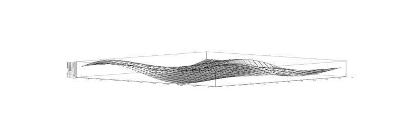
Figure 1: The graph of the Green’s function $G(x,t,\mu)$ for $\mu=3$

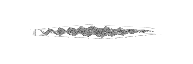
Figure 2: The graph of the Green’s function $G(x,t,\mu)$ for $\mu=15$

The graph of the Green’s function is displayed in Figure 1 and Figure 2 for two different values of spectral parameter.

References

• [1] D. G. Duffy, Green’s Functions with Applications , Chapmanand Hall/Crc, 2001.
• [2] J. Ao, J. Sun and M. Zhang, Matrix representations of Sturm-Liouville problems with transmission conditions, Comput. Math. Appl., 63(2012), 1335-1348.
• [3] B. M. Levitan and I. S. Sargsyan, Sturm - Liouville and Dirac Operators, Springer-Verlag New York, 1991.
• [4] A. V. Likov and Yu. A. Mikhailov, The theory of Heat and Mass Transfer, Qosenergaizdat, 1963(Russian).
• [5] O. Sh. Mukhtarov and H. Demir, Coersiveness of the discontinuous initial- boundary value problem for parabolic equations, Israel J. Math., Vol. 114(1999), Pages 239-252.
• [6] O. Sh. Mukhtarov and M. Kadakal Some spectral properties of one Sturm-Liouville type problem with discontinuous weight, Sib. Math. J., 46(2005), 681-694.
• [7] F. S. Muhtarov and K. AydemirDistributions of eigenvalues for Sturm-Liouville problem under jump conditions, Journal of New Results in Science 1(2012) 81-89.
• [8] O. Sh. Mukhtarov and S. Yakubov, Problems for ordinary differential equations with transmission conditions, Appl. Anal.,81(2002),1033-1064.
• [9] M. L. Rasulov, Methods of Contour Integration, North-Holland Publishing Company, Amsterdam, 1967.
• [10] A. N. Tikhonov and A. A. Samarskii, Equations of Mathematical Physics, Oxford and New York, Pergamon, 1963.
• [11] E. C. Titchmarsh, Eigenfunctions Expansion Associated with Second Order Differential Equations I, second edn. Oxford Univ. Press, London, 1962.
• [12] I. Titeux and Ya. Yakubov, Completeness of root functions for thermal conduction in a strip with piecewise continuous coefficients, Math. Models Methods Appl. Sc., 7(7), (1997), 1035-1050.
• [13] N. N. Voitovich , B. Z. Katsenelbaum and A. N. Sivov , Generalized Method of Eigen-vibration in the theory of Diffraction , Nakua, Mockow, 1997 (Russian).