Wave front propagation for a reaction-diffusion equation in narrow random channels

Abstract

We consider a reaction-diffusion equation in narrow random channels. We approximate the generalized solution to this equation by the corresponding one on a random graph. By making use of large deviation analysis we study the asymptotic wave front propagation.

Keywords: reaction-diffusion equation, wave front propagation, diffusion processes on graphs, random environment.

2010 Mathematics Subject Classification Numbers: 35K57, 35A18, 60J60, 60K37.

1 Introduction

In studying the motion of molecular motors we introduced in [5] a solvable model: we think of the molecular motors as diffusion particles traveling in a narrow random channel. Based on the model suggested in [5], we consider in this paper wave front propagation for a reaction-diffusion in narrow random channels. Problems of this type naturally appear in the theory of nerve impulse propagation and in combustion theory. Our analysis relies on techniques in large deviations similar to that of [3, Chapter 7] and [14], [13], [15], [1], [18, Chapter 5]. We shall note that problems of this type are mentioned in [4, Chapter 7], [8], [7]. It is also interesting to note that similar problems are considered in [12], [16], [17] but from different points of view.

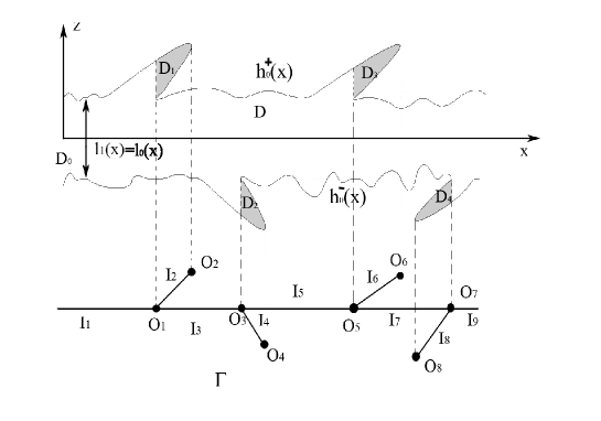
Fig. 1: A model of the molecular motor.

Let us first briefly recall the model introduced in [5]. Let $h_{0}^{\pm}(x)$ be a pair of piecewise smooth functions with $h_{0}^{+}(x)-h_{0}^{-}(x)=l_{0}(x)>0$. Let $D_{0}=\{(x,z):x\in\mathbb{R},h_{0}^{-}(x)\leq z\leq h_{0}^{+}(x)\}$ be a tubular $2$-d domain of infinite length, i.e. it goes along the whole $x$-axis. At the discontinuities of $h_{0}^{\pm}(x)$, we connect the pieces of the boundary via straight vertical lines. The domain $D_{0}$ models the ”main” channel in which the motor is traveling. Let a sequence of ”wings” $D_{j}$ ($j\geq 1$) be attached to $D_{0}$. These wings are attached to $D_{0}$ at the discontinuities of the functions $h_{0}^{\pm}(x)$.

Consider the union $D=D_{0}\bigcup\left(\bigcup\limits_{j=1}^{\infty}D_{j}\right)$. An example of such a domain $D$ is shown in Fig.1, in which one can see four ”wings” $D_{1},D_{2},D_{3},D_{4}$. We assume that, after adding the ”wings”, for the domain $D$, the boundary $\partial D$ has two smooth pieces: the upper boundary and the lower boundary. Let $\boldsymbol{n}(x,z)=(n_{1}(x,z),n_{2}(x,z))$ be the inward unit normal vector to $\partial D$. We make same assumptions as in [5].

Assumption 1. The set of points $x\in\mathbb{R}$ for which there are points $(x,z)\in\partial D$ at which the unit normal vector $\boldsymbol{n}(x,z)$ is parallel to the $x$-axis: $n_{2}(x,z)=0$ has no limit points in $\mathbb{R}$. Each such point $x$ corresponds to only one point $(x,z)\in\partial D$ for which $n_{2}(x,z)=0$.

Assumption 2. For every $x$ the cross-section of the region $D$ at level $x$, i.e., the set of all points belonging to $D$ with the first coordinate equal to $x$, consists of either one or two intervals that are its connected components. That is to say, in the case of one interval this interval corresponds to the ”main channel” $D_{0}$; and in the case of two intervals one of them corresponds to the ”main channel” $D_{0}$ and the other one corresponds to the wing. The wing will not have additional branching structure. Also, for some $0<l_{0}<\bar{l}_{0}<\infty$ we have $\l_{0}\leq h_{0}^{+}(x)-h_{0}^{-}(x)=l_{0}(x)\leq\bar{l}_{0}$.

Let us take into account randomness of the domain $D$. Keeping the above assumptions in mind, we can assume that the functions $h_{0}^{\pm}(x)$ and the shape of the wings $D_{k}$ ($k=1,2,...$) are all random. Thus we can view the shape of $D$ as random. We introduce a filtration $\mathcal{F}_{s}^{t}$, $-\infty\leq s<t\leq\infty$ as the smallest $\sigma$-algebra corresponding to the shape of $D\cap\{(x,z):x\in[s,t]\}$. We introduce stationarity and mixing assumptions. Let us consider some $A\in\mathcal{F}_{s}^{t}$, $-\infty\leq s<t\leq\infty$. The set $A$ consists of some shapes of the domain $D\cap\{(x,z):x\in[s,t]\}$. Let $\theta_{r}$ ($r\in\mathbb{R}$) be the operator corresponding to the shift along $x$-direction: $\theta_{r}(A)\in\mathcal{F}_{s+r}^{t+r}$ consists of the same shapes as those in $A$ but correspond to the domain $D\cap\{(x,z):x\in[s+r,t+r]\}$.

Assumption 3. (stationarity) We have $\mathbf{P}(A)=\mathbf{P}(\theta_{r}(A))$.

Assumption 4. (mixing) For any $A\in\mathcal{F}_{s}^{t}$ and any $B\in\mathcal{F}_{s+r}^{t+r}$ we have

$$\lim\limits_{r\rightarrow\pm\infty}\sup\limits_{A\in\mathcal{F}_{s}^{t},B\in\mathcal{F}_{s+r}^{t+r}}|\mathbf{P}(A\cap B)-\mathbf{P}(A)\mathbf{P}(B)|=0$$

exponentially fast.

For instance, we can assume that there exists some $M>0$ such that $\mathbf{P}(A\cap B)=\mathbf{P}(A)\mathbf{P}(B)$ for $|r|\geq M$.

In particular, the mixing assumption implies that the transformation $\theta_{r}$ is ergodic.

Here and below the symbols $\mathbf{P}$ and $\mathbf{E}$ etc. refer to probabilities and expectations etc. with respect to the filtration $\{\mathcal{F}_{s}^{t}\}_{-\infty\leq s<t\leq\infty}$.

Let $D^{\varepsilon}=\{(x,\varepsilon z):(x,z)\in D\}$. The parameter $\varepsilon>0$ is small. The domain $D^{\varepsilon}$ models the narrow random channel. Let us consider the following reaction-diffusion equation in the domain $D^{\varepsilon}$:

$$\left\{\begin{array}[]{l}\dfrac{\partial u^{\varepsilon}}{\partial t}=\dfrac{1}{2}\left(\dfrac{\partial^{2}u^{\varepsilon}}{\partial x^{2}}+\dfrac{\partial^{2}u^{\varepsilon}}{\partial z^{2}}\right)+V(x,z)\dfrac{\partial u^{\varepsilon}}{\partial x}+f(u^{\varepsilon})\ ,\\ u^{\varepsilon}(0,x,z)=g(x)\ ,\\ \left.\dfrac{\partial u^{\varepsilon}}{\partial\nu}\right|_{\partial D^{\varepsilon}}=0\ ,\\ u^{\varepsilon}=u^{\varepsilon}(t,x,z)\ ,\ (t,x,z)\in\mathbb{R}_{+}\times D^{\varepsilon}\ .\end{array}\right.$$

Here $\nu$ is the inward unit normal vector field on $\partial D^{\varepsilon}$; $V(x,z)$ is the velocity field; the function $f(u^{\varepsilon})$ is smooth and is of KPP type: $f\in\mathbf{C}^{(\infty)}([0,1])$, $f(0)=f(1)$, $0\leq f(u^{\varepsilon})\leq f^{\prime}(0)u^{\varepsilon}$ for all $u^{\varepsilon}\in(0,1)$, e.g. $f(u^{\varepsilon})=u^{\varepsilon}(1-u^{\varepsilon})$. The initial function $g(x)\geq 0$ (not identically equal to $0$) is smooth and compactly supported in $x\in\mathbb{R}$: $g(x)\in\mathbf{C}^{(\infty)}_{0}(\mathbb{R})$. We notice that the initial function $g(x)$ depends only on the variable $x\in\mathbb{R}$ and is independent of $z$.

Alternatively, problem (1.1) can be considered on the domain $D$ with a change of variable $z\mapsto z/\varepsilon$. The equivalent problem takes the form

$$\left\{\begin{array}[]{l}\dfrac{\partial u^{\varepsilon}}{\partial t}=\dfrac{1}{2}\left(\dfrac{\partial^{2}u^{\varepsilon}}{\partial x^{2}}+\dfrac{1}{\varepsilon^{2}}\dfrac{\partial^{2}u^{\varepsilon}}{\partial z^{2}}\right)+V(x,z)\dfrac{\partial u^{\varepsilon}}{\partial x}+f(u^{\varepsilon})\ ,\\ u^{\varepsilon}(0,x,z)=g(x)\ ,\\ \left.\dfrac{\partial u^{\varepsilon}}{\partial\nu^{\varepsilon}}\right|_{\partial D}=0\ ,\\ u^{\varepsilon}=u^{\varepsilon}(t,x,z)\ ,\ (t,x,z)\in\mathbb{R}_{+}\times D\ .\end{array}\right.$$

Here $\nu^{\varepsilon}=(\nu^{\varepsilon}_{1},\nu^{\varepsilon}_{2})=(\varepsilon n_{1}(x,z),n_{2}(x,z))$ is the inward unit co-normal vector field on $\partial D$ corresponding to the operator $\dfrac{1}{2}\left(\dfrac{\partial^{2}}{\partial x^{2}}+\dfrac{1}{\varepsilon^{2}}\dfrac{\partial^{2}}{\partial z^{2}}\right)$.

The diffusion process $\boldsymbol{X}_{t}^{\varepsilon}=(X_{t}^{\varepsilon},Z_{t}^{\varepsilon})$ corresponding to problem (1.2) takes the form of equation (2) in [5]. We have

$$\left\{\begin{array}[]{l}dX_{t}^{\varepsilon}=dW_{t}^{1}+V(X_{t}^{\varepsilon},Z_{t}^{\varepsilon})dt+\nu_{1}^{\varepsilon}(X_{t}^{\varepsilon},Z_{t}^{\varepsilon})d\ell_{t}^{\varepsilon}\ ,\\ dZ_{t}^{\varepsilon}=\dfrac{1}{\varepsilon}dW_{t}^{2}+\nu_{2}^{\varepsilon}(X_{t}^{\varepsilon},Z_{t}^{\varepsilon})d\ell_{t}^{\varepsilon}\ ,\end{array}\right.$$

Let $\mathbf{P}^{W}$, $\mathbf{E}^{W}$ denote probabilities and expectations with respect to the filtration generated by $\boldsymbol{X}_{t}^{\varepsilon}$ (and henceforth $(W_{t}^{1},W_{t}^{2})$). We note that as in [5] the motion of $\boldsymbol{X}_{t}^{\varepsilon}$ is independent of the random shape of $D$ (and henceforth $D^{\varepsilon}$). We have, in the same way as [5], the following.

Assumption 5. The process $(W_{t}^{1},W_{t}^{2})$ is independent of the filtration $\{\mathcal{F}_{s}^{t}\}_{-\infty\leq s<t\leq\infty}$ corresponding to the shape of $D$.

We shall also make some assumptions parallel to Assumptions 7 and 8 in [5]. To this end we let $L$ be the random variable distributed the same as the distance along $x$-axis between two wings: $L$ is the distance along $x$-axis between two cross-sections of $D$ where there is a branching. Let $l_{\text{wing}}$ be the cross-section width of the wing. Let $r$ be the projection length of a wing onto $x$-axis ($r$ can be positive or negative; compare with [5, Assumptions 7 and 8]). We assume the following.

Assumption 6. With $\mathbf{P}$ probability $1$ we have (1) $+\infty>\overline{L}\geq L\geq\underline{L}>0$ for some constants $\overline{L},\underline{L}>0$; (2) $0\leq l_{\text{wing}}(x)\leq A_{1}$ and $|r|\leq A_{1}$ for some constant $A_{1}>0$.

Our goal in this paper is to study the asymptotic wave front propagation properties for the generalized solution of (1.2). To be precise, by a generalized solution of (1.2) we mean the one defined via the path integral representation (Feynmann-Kac) formula:

$$u^{\varepsilon}(t,(x,z))=\mathbf{E}_{(x,z)}^{W}\left[\exp\left(\int_{0}^{t}c(u^{\varepsilon}(t-s,\boldsymbol{X}_{s}^{\varepsilon}))ds\right)g(X_{t}^{\varepsilon})\right]\ .$$

Here $c(u)=\dfrac{f(u)}{u}$ for $u>0$ and $c(0)=\lim\limits_{u\downarrow 0}\dfrac{f(u)}{u}=\sup\limits_{u>0}\dfrac{f(u)}{u}$. The latter equality is due to the KPP nonlinearity assumption. We shall also suppose that $|c^{\prime}(u)|\leq\text{Lip}(c)<\infty$, $u\in[0,1]$. The proof of existence, uniqueness and regularity of the generalized solution to the integral equation (1.3) is close to [3, Chapter 5, Section 3]. For the reader’s convenience we will prove it in Section 3 of this paper.

We introduced in [5] the metric graph $\Gamma$ corresponding to the domain $D$ (see Fig.1). Let $Y_{t}=(X_{t},k_{t})$ be defined on $\Gamma$ as in [5, Section 2]. The construction of the graph $\Gamma$ and the process $Y_{t}$ as well as some basic convergence results in [5] will be recalled in Section 2. The process $Y_{t}$ is a diffusion process on $\Gamma$ with a generator $A$ and the domain of definition $D(A)$. We consider the reaction-diffusion equation associated with the Markov process $Y_{t}$. This equation takes the form

$$\dfrac{\partial u}{\partial t}=Au+f(u)\ ,\ u(0,(x,k))=g(x)\ ,\ u=u(t,y),\ (t,y)\in\mathbb{R}_{+}\times\Gamma\ .$$

The initial function $g=g(x)$ is the same as in (1.2). We require that for each fixed $t\geq 0$, $u(t,\bullet)\in D(A)$. This requirement ia a kind of boundary condition. For details we refer to [5] and [9, Chapter 8] and the references therein.

The generalized solution to (1.4) is defined as the solution to the integral equation

$$u(t,(x,k))=\mathbf{E}_{(x,k)}^{W}\left[\exp\left(\int_{0}^{t}c(u(t-s,Y_{s}))ds\right)g(X_{t})\right]\ .$$

The existence and regularity of the solution can be proved in a same way as those for (1.3). We will briefly mention this in Section 3.

We will show, in Section 3 of this paper, that as $\varepsilon\downarrow 0$, the solution $u^{\varepsilon}(t,(x,z))$ of (1.3) will converge to $u(t,(x,k))$ of (1.5) in the strong sense. Here $(x,k)=\mathbf{\mathfrak{Y}}((x,z))$ and the mapping $\mathbf{\mathfrak{Y}}:D\rightarrow\Gamma$ is an identification map that will be recalled in Section 2.

After we get convergence results we will focus on the study of the solution $u(t,(x,k))$ of (1.5). We will show that, as $t\rightarrow\infty$, the solution $u(t,(x,k))$ behaves asymptotically as a traveling wave. This wave is traveling in both positive and negative directions along $x$-axis.

The paper is organized as follows: in Section 2 we recall some necessary basic set up of [5], such as the construction of the graph $\Gamma$, the process $Y_{t}$, etc.; in Section 3 we show the convergence as $\varepsilon\downarrow 0$ of the solution $u^{\varepsilon}(t,(x,z))$ to $u(t,(x,k))$; in Section 4 we obtain some auxiliary results that will be used in later sections; in Section 5 we derive the large deviation principle; in Section 6 we study the wave front propagation properties of the solution $u(t,(x,k))$.

2 Set up

We shall first recall some basic facts in [5] (also see [10]). Let us work with a fixed shape of $D$.

First of all we need to construct a graph $\Gamma$ related to the domain $D$ (see Fig.1). For $x_{0}\in\mathbb{R}$, let $C(x_{0})=\{(x,z)\in D:x=x_{0}\}$ be the intersection of the domain $D$ with the line $\{x=x_{0}\}$. The set $C(x_{0})$ may have several connected components. We identify all points in each connected component and the set thus obtained, equipped with the natural topology, is homeomorphic to a graph $\Gamma$. We label the edges of this graph $\Gamma$ by $I_{1},...,I_{k},...$ (there might be infinitely many such edges).

We see that the structure of the graph $\Gamma$ consists of many edges (such as $I_{1},I_{3},I_{5},I_{7},I_{9}$,… in Fig.1) that form a long line corresponding to the domain $D_{0}$ and many other short edges (such as $I_{2},I_{4},I_{6},I_{8}$,… in Fig.1) attached to the long line in a random way. We will henceforth denote by $I_{0}$ the long line corresponding to the domain $D_{0}$.

A point $y\in\Gamma$ can be characterized by two coordinates: the horizontal coordinate $x$, and the discrete coordinate $k$ being the number of the edge $I_{k}$ in the graph $\Gamma$ to which the point $y$ belongs. Let the identification mapping be $\mathfrak{Y}:D\rightarrow\Gamma$. We note that the second coordinate is not chosen in a unique way: for $y$ being an interior vertex $O_{i}$ of the graph $\Gamma$ we can take $k$ to be the number of any of the several edges meeting at the vertex $O_{i}$.

The distance $\rho(y_{1},y_{2})$ between two points $y_{1}=(x_{1},k)$ and $y_{2}=(x_{2},k)$ belonging to the same edge of the graph $\Gamma$ is defined as $\rho(y_{1},y_{2})=|x_{1}-x_{2}|$; for $y_{1},y_{2}\in\Gamma$ belonging to different edges of the graph it is defined as the geodesic distance $\rho(y_{1},y_{2})=\min(\rho(y_{1},O_{j_{1}})+\rho(O_{j_{1}},O_{j_{2}})+...+\rho(O_{j_{l}},y_{2}))$, where the minimum is taken over all chains $y_{1}\leftrightarrow O_{j_{1}}\leftrightarrow O_{j_{2}}\leftrightarrow...\leftrightarrow O_{j_{l}}\leftrightarrow y_{2}$ of vertices $O_{j_{i}}$ connecting the points $y_{1}$ and $y_{2}$.

For an edge $I_{k}=\{(x,k):A_{k}\leq x\leq B_{k}\}$ we consider the ”tube” $U_{k}=\mathbf{\mathfrak{Y}}^{-1}(I_{k})\cap\{A_{k}\leq x\leq B_{k}\}$ in $D$. The ”tube” $U_{k}$ can be characterized by the interval $x\in[A_{k},B_{k}]$ and the ”height functions” $h_{k}^{\pm}(x)$: $U_{k}=\{(x,z):A_{k}\leq x\leq B_{k},h_{k}^{-}(x)\leq z\leq h_{k}^{+}(x)\}$. For $x\in[A_{k},B_{k}]$, we denote the set $C_{k}(x)$ to be the connected component of $C(x)$ that corresponds to the ”tube” $U_{k}$: $C_{k}(x)=\{x\}\times[h_{k}^{-},h_{k}^{+}]$. Let $l_{k}(x)=h_{k}^{+}(x)-h_{k}^{-}(x)\geq 0$ for all $x\in\mathbb{R}$. We notice that each $h_{k}^{\pm}(x),l_{k}(x)$, etc. is smooth.

The vertices $O_{j}$ correspond to the connected components containing points $(x,z)\in\partial D$ with $n_{2}(x,z)=0$. There are two types of vertices: the interior vertices (in Fig.1 they are $O_{1},O_{3},O_{5},O_{7}$) are the intersection of three edges; the exterior vertices (in Fig.1 they are $O_{2},O_{4},O_{6},O_{8}$) are the endpoints of only one edge.

Using the ideas in [10] with a little modification we can establish the weak convergence of the process $Y_{t}^{\varepsilon}=\mathbf{\mathfrak{Y}}(\boldsymbol{X}_{t}^{\varepsilon})$ (which is not Markov in general) as $\varepsilon\downarrow 0$ in the space $\mathbf{C}_{[0,T]}(\Gamma)$ to a certain Markov process $Y_{t}$ on $\Gamma$. A sketch of the proof of this fact is in [5, Section 2].

The process $Y_{t}$ is a diffusion process on $\Gamma$ with a generator $A$ and the domain of definition $D(A)$. We are going now to define the operator $A$ and its domain of definition $D(A)$.

For each edge $I_{k}$ we define an operator $\overline{L}_{k}$:

$$\overline{L}_{k}u(x)=\dfrac{1}{2l_{k}(x)}\dfrac{d}{dx}\left(l_{k}(x)\dfrac{du}{dx}\right)+\overline{V}_{k}(x)\dfrac{du}{dx}\ ,\ A_{k}\leq x\leq B_{k}\ .$$

Here

$$\overline{V}_{k}(x)=\dfrac{1}{l_{k}(x)}\int_{h_{k}^{-}(x)}^{h_{k}^{+}(x)}V(x,z)dz$$

is the average of the velocity field $V(x,z)$ on the connected component $C_{k}(x)$, with respect to Lebesgue measure in $z$-direction. At places where $l_{k}=0$, the above expression for $\overline{V}_{k}(x)$ is understood as a limit as $l_{k}\rightarrow 0$:

$$\overline{V}_{k}(x)=\lim\limits_{y\rightarrow x}\dfrac{1}{l_{k}(y)}\int_{h_{k}^{-}(y)}^{h_{k}^{+}(y)}V(y,z)dz\ .$$

We will assume throughout this paper the following.

Assumption 7. The function $\overline{V}_{k}(x)=0$.

We notice that this is a bit different from the corresponding one in [5, Assumption 6]. We point out that the vanishing mean drift assumption is crucial for the method of our analysis to work.

Thus under our Assumption 7 we have

$$\overline{L}_{k}u(x)=\displaystyle{\dfrac{1}{2l_{k}(x)}\dfrac{d}{dx}\left(l_{k}(x)\dfrac{du}{dx}\right)}\ .$$

The operator $\overline{L}_{k}$ can be represented as a generalized second order differential operator (see [2])

$$\overline{L}_{k}u(x)=D_{m_{k}}D_{p_{k}}f(x)\ ,$$

where, for an increasing function $h$, the derivative $D_{h}$ is defined by $D_{h}g(x)=\lim\limits_{\delta\downarrow 0}\dfrac{g(x+\delta)-g(x)}{h(x+\delta)-h(x)}$, and

$$p_{k}(x)=\int\dfrac{dx}{l_{k}(x)}$$

is the scale function,

$$m_{k}(x)=2\int l_{k}(x)dx$$

is the speed measure.

The operator $A$ is acting on functions $f$ on the graph $\Gamma$: for $y=(x,k)$ being an interior point of the edge $I_{k}$ we take $Af(y)=\overline{L}_{k}f(x,k)$.

The domain of definition $D(A)$ of the operator $A$ consists of such functions $f$ satisfying the following properties.

$\bullet$ The function $f$ is a continuous function that is twice continuously differentiable in $x$ in the interior part of every edge $I_{k}$;

$\bullet$ There exist finite limits $\lim\limits_{y\rightarrow O_{i}}Af(y)$ (which are taken as the value of the function $Af$ at the point $O_{i}$);

$\bullet$ There exist finite one-sided limits $\lim\limits_{x\rightarrow x_{i}}D_{p_{k}}f(x,k)$ along every edge ending at $O_{i}=(x_{i},k)$ and they satisfy the gluing conditions

$$\sum\limits_{j=1}^{N_{i}}(\pm)\lim\limits_{x\rightarrow x_{i}}D_{p_{k_{j}}}f(x,k_{j})=0\ ,$$

where the sign ”$+$” is taken if the values of $x$ for points $(x,k_{j})\in I_{k_{j}}$ are $\geq x_{i}$ and ”$-$” otherwise. Here $N_{i}=1$ (when $O_{i}$ is an exterior vertex) or $3$ (when $O_{i}$ is an interior vertex).

For an exterior vertex $O_{i}=(x_{i},k)$ with only one edge $I_{k}$ attached to it the condition (2.1) is just $\lim\limits_{x\rightarrow x_{i}}D_{p_{k}}f(x,k)=0$. Such a boundary condition can also be expressed in terms of the usual derivatives $\dfrac{d}{dx}$ instead of $D_{p_{k}}$. It is $\lim\limits_{x\rightarrow x_{i}}l_{k}(x)\dfrac{\partial f}{\partial x}(x,k)=0$. We remark that we are in dimension 2 so that these exterior vertices are accessible, and the boundary condition can be understood as a kind of (not very standard) instantaneous reflection. In dimension 3 or higher these endpoints do not need a boundary condition, they are just inaccessible. For an interior vertex the gluing condition (2.1) can be written with the derivatives $\dfrac{d}{dx}$ instead of $D_{p_{k}}$. For $k$ being one of the $k_{j}$ we define $\alpha_{ik}=\lim\limits_{x\rightarrow x_{i}}l_{k}(x)$ (for each edge $I_{k}$ the limit is a one-sided one). Then the condition (2.1) can be written as

$$\sum\limits_{j=1}^{3}(\pm)\alpha_{i,k_{j}}\cdot\lim\limits_{x\rightarrow x_{i}}\dfrac{df(x,k_{j})}{dx}=0\ .$$

It can be shown as in [10, Section 2] that the process $Y_{t}$ exists as a continuous strong Markov process on $\Gamma$.

We fix the shape of $D$. For every $\varepsilon>0$, every $\boldsymbol{x}=(x,z)\in D$ and every $T\in(0,\infty)$ let us consider the distribution $\mu_{\boldsymbol{x}}^{\varepsilon}$ of the trajectory $Y_{t}^{\varepsilon}=\mathbf{\mathfrak{Y}}(\boldsymbol{X}_{t}^{\varepsilon})$ starting from a point $\boldsymbol{X}_{0}^{\varepsilon}=\boldsymbol{x}$ in the space $\mathbf{C}_{[0,T]}(\Gamma)$ of continuous functions on the interval $[0,T]$ with values in $\Gamma$: the probability measure defined for every Borel subset $B\subseteq\mathbf{C}_{[0,T]}(\Gamma)$ as $\mu_{\boldsymbol{x}}^{\varepsilon}(B)=\mathbf{P}_{\boldsymbol{X}_{0}^{\varepsilon}=\boldsymbol{x}}^{W}(Y_{\bullet}^{\varepsilon}\in B)$. Similarly, for every $y\in\Gamma$ and $T>0$ let $\mu^{0}_{y}$ be the distribution of the process $Y_{t}$ in the same space: $\mu^{0}_{y}(B)=\mathbf{P}^{W}_{y}(Y_{\bullet}\in B)$. The following theorem is basic for our analysis.

Theorem 2.1. For every $\boldsymbol{x}\in D$ and every $T>0$ the distribution $\mu_{\boldsymbol{x}}^{\varepsilon}$ converges weakly to $\mu_{\mathbf{\mathfrak{Y}}(\boldsymbol{x})}^{0}$ as $\varepsilon\downarrow 0$.

In other words we have

$$\mathbf{E}_{\boldsymbol{X}_{0}^{\varepsilon}=\boldsymbol{x}}^{W}F(Y^{\varepsilon}_{\bullet})\rightarrow\mathbf{E}_{\mathbf{\mathfrak{Y}}(\boldsymbol{x})}^{W}F(Y_{\bullet})$$

for every bounded continuous functional $F$ on the space $\mathbf{C}_{[0,T]}(\Gamma)$.

The proof of this theorem follows from [10] and there is a sketch in [5, Section 3]. We omit duplicating the details here.

3 Convergence of $u^{\varepsilon}$ to $u$

We recall that our definition of the generalized solutions to (1.2) and (1.4) are the solutions of the integral equations (1.3) and (1.5), respectively. That is to say, we have

$$u^{\varepsilon}(t,(x,z))=\mathbf{E}_{(x,z)}^{W}\left[\exp\left(\int_{0}^{t}c(u^{\varepsilon}(t-s,\boldsymbol{X}_{s}^{\varepsilon}))ds\right)g(X_{t}^{\varepsilon})\right]$$

and

$$u(t,(x,k))=\mathbf{E}_{(x,k)}^{W}\left[\exp\left(\int_{0}^{t}c(u(t-s,Y_{s}))ds\right)g(X_{t})\right]\ .$$

Theorem 3.1. There exist unique bounded measurable generalized solutions $u^{\varepsilon}(t,(x,z))$, $t>0,(x,z)\in D$ and $u(t,(x,k))$, $t>0,(x,k)\in\Gamma$ for (1.2) and (1.4), respectively. These solutions are continuous for all $t\geq 0$.

Proof. We take (1.2) as an example. The proof for (1.4) is exactly the same. We shall prove the existence and regularity by using a contraction mapping principle (compare with [3, §5.3]). To this end we consider the Banach space $B_{T}$ of bounded measurable functions on $[0,T]\times[D]$ with norm $\|v\|=\sup\limits_{(t,x)\in[0,T]\times[D]}|v(t,x)|$. Consider in $B_{T}$ the following operator

$$F[v]=F[v](t,(x,z))=\mathbf{E}_{(x,z)}^{W}\left[\exp\left(\int_{0}^{t}c(v(t-s,\boldsymbol{X}_{s}^{\varepsilon}))ds\right)g(X_{t}^{\varepsilon})\right]\ ,\ v\in B_{T}\ .$$

It is then checked that we have, for $0\leq t\leq T_{0}\leq T$, that

$$\begin{array}[]{l}|F[u]-F[v]|(t,(x,z))\\ \displaystyle{=\left|\mathbf{E}_{(x,z)}^{W}\left[\exp\left(\int_{0}^{t}c(u(t-s,\boldsymbol{X}_{s}^{\varepsilon}))ds\right)g(X_{t}^{\varepsilon})\right]-\mathbf{E}_{(x,z)}^{W}\left[\exp\left(\int_{0}^{t}c(v(t-s,\boldsymbol{X}_{s}^{\varepsilon})ds\right)g(X_{t}^{\varepsilon})\right]\right|}\\ \displaystyle{\leq\|g\|\left|\mathbf{E}_{(x,z)}^{W}\left[\exp\left(\int_{0}^{t}c(u(t-s,\boldsymbol{X}_{s}^{\varepsilon}))ds\right)-\exp\left(\int_{0}^{t}c(v(t-s,\boldsymbol{X}_{s}^{\varepsilon}))ds\right)\right]\right|}\\ \displaystyle{\leq\|g\|\exp(c(0)t)\cdot\text{Lip}(c)\cdot t\cdot\|u-v\|}\\ =C(T_{0})\|u-v\|\end{array}$$

for $u,v\in B_{t}$ and $C(T_{0})=\|g\|\exp(c(0)T_{0})\text{Lip}(c)T_{0}$. This guarantees that $F$ is a contraction provided that $T_{0}<\dfrac{1}{\|g\|\text{Lip}(c)\exp(c(0)T)}$. By contraction mapping theorem we have existence and uniqueness of generalized solution in the space of bounded measurable functions to the problem (1.2) on the interval $[0,T_{0}]$. Since the solution $|u^{\varepsilon}(T_{0},(x,z))|\leq\|g\|\exp(c(0)T_{0})$ we can use the same $T_{0}$ and work with intervals $[T_{0},2T_{0}]$, …, up to $[(k-1)T_{0},kT_{0}]$ ($k\geq 1$) provided that $kT_{0}<T$. This gives existence ”in the large” for a unique generalized solution $u^{\varepsilon}(t,(x,z))$ for (1.2) in the space of bounded measurable functions.

The continuity of the solution $u^{\varepsilon}(t,(x,z))$ in the variables $t$ and $(x,z)$ is provided by (1) The continuity of $g$; (2) The Lipschitz continuity of $c(u)$; (3) The continuity and continuous dependence of the process $\boldsymbol{X}_{t}^{\varepsilon}$ on $\boldsymbol{X}_{0}^{\varepsilon}=(x,z)$. $\square$

We shall then show the approximation of the generalized solution $u^{\varepsilon}(t,(x,z))$ as $\varepsilon$ is small by the generalized solution $u(t,\mathbf{\mathfrak{Y}}((x,z)))$. We prove this via a sequence of auxiliary results.

Lemma 3.1. We have

$$\lim\limits_{\varepsilon\downarrow 0}\max\limits_{(x,z_{1}),(x,z_{2})\in\mathbf{\mathfrak{Y}}^{-1}((x,k))}\max\limits_{0\leq t\leq T}|u^{\varepsilon}(t,(x,z_{1}))-u^{\varepsilon}(t,(x,z_{2}))|=0\ .$$

Proof. We consider the stopping time $\tau^{\varepsilon}=\tau^{\varepsilon}((x,z_{2}),z_{1})=\inf\{t>0:X_{0}^{\varepsilon}=x,Z_{0}^{\varepsilon}=z_{2},Z_{t}^{\varepsilon}=z_{1}\}$. By strong Markov property of the process $\boldsymbol{X}_{t}^{\varepsilon}$ we have

$$\begin{array}[]{l}u^{\varepsilon}(t,(x,z_{2}))\\ =\displaystyle{\mathbf{E}_{(x,z_{2})}^{W}\left[\exp\left(\int_{0}^{t}c(u^{\varepsilon}(t-s,X_{s}^{\varepsilon},Z_{s}^{\varepsilon}))ds\right)g(X_{t}^{\varepsilon})\right]}\\ =\displaystyle{\mathbf{E}_{(x,z_{2})}^{W}\left[\exp\left(\int_{0}^{\tau^{\varepsilon}}c(u^{\varepsilon}(t-s,X_{s}^{\varepsilon},Z_{s}^{\varepsilon}))ds\right)u^{\varepsilon}(t-\tau^{\varepsilon},(X_{\tau^{\varepsilon}}^{\varepsilon},z_{1}))\right]}\ .\end{array}$$

Since the motion $Z_{t}^{\varepsilon}$ is moving very fast as $\varepsilon\downarrow 0$ we see that $\tau^{\varepsilon}\rightarrow 0$ almost surely as $\varepsilon\downarrow 0$. This immediately implies the convergence. $\square$

Let $(x,k)\in\Gamma$. We introduce a new function

$$\bar{u}^{\varepsilon}(t,(x,k))=\dfrac{1}{|\mathbf{\mathfrak{Y}}^{-1}((x,k))|}\displaystyle{\int_{\mathbf{\mathfrak{Y}}^{-1}((x,k))}u^{\varepsilon}(t,(x,z))dz}\ ,$$

and we see from Lemma 3.1 that we have the following.

Corollary 3.1. We have

$$\lim\limits_{\varepsilon\downarrow 0}\max\limits_{(x,z)\in\mathbf{\mathfrak{Y}}^{-1}((x,k))}\max\limits_{0\leq t\leq T}|\bar{u}^{\varepsilon}(t,\mathbf{\mathfrak{Y}}(x,z))-u^{\varepsilon}(t,(x,z))|=0\ .$$

We are going now to prove that the function $\bar{u}^{\varepsilon}(t,(x,k))$ has a uniform in $\varepsilon$ bounded first derivative in the variable $x$.

Lemma 3.2. We have an a-priori estimate

$$\max\limits_{0\leq t\leq T,(x,k)\in\Gamma}\left|\dfrac{\partial\bar{u}^{\varepsilon}}{\partial x}(t,(x,k))\right|\leq C(T)=C$$

where $C>0$ is independent of $\varepsilon$.

Proof. By (1.3) we have

$$u^{\varepsilon}(t,(x,z))=\mathbf{E}_{(x,z)}^{W}\left[\exp\left(\int_{0}^{t}c(u^{\varepsilon}(t-s,\boldsymbol{X}_{t}^{\varepsilon}))ds\right)g(X_{t}^{\varepsilon})\right]\ .$$

Differentiating with respect to $x$ we have

$$\begin{array}[]{l}\displaystyle{\dfrac{\partial u^{\varepsilon}}{\partial x}=\mathbf{E}^{W}\left[\dfrac{\partial g}{\partial x}(X_{t}^{\varepsilon})\dfrac{\partial X_{t}^{\varepsilon}}{\partial x}\exp\left(\int_{0}^{t}c(u^{\varepsilon}(t-s,X_{s}^{\varepsilon},Z_{s}^{\varepsilon}))ds\right)\right.}\\ \displaystyle{\left.\ \ \ +g(X_{t}^{\varepsilon})\exp\left(\int_{0}^{t}c(u^{\varepsilon}(t-s,X_{s}^{\varepsilon},Z_{s}^{\varepsilon}))\right)\dfrac{\partial}{\partial x}\left(\int_{0}^{t}c(u^{\varepsilon}(t-s,X_{s}^{\varepsilon},Z_{s}^{\varepsilon}))ds\right)\right]}\ .\end{array}$$

Note that

$$\dfrac{\partial}{\partial x}\left(\int_{0}^{t}c(u^{\varepsilon}(t-s,X_{s}^{\varepsilon},Z_{s}^{\varepsilon}))ds\right)=\int_{0}^{t}c^{\prime}(u^{\varepsilon}(t-s,X_{s}^{\varepsilon},Z_{s}^{\varepsilon}))\dfrac{\partial u^{\varepsilon}}{\partial x}(t-s,X_{s}^{\varepsilon},Z_{s}^{\varepsilon})\dfrac{\partial X_{s}^{\varepsilon}}{\partial x}ds\ .$$

Therefore if we let $m^{\varepsilon}(t)=\max\limits_{(x,k)\in D,0\leq s\leq t}\left|\dfrac{\partial u^{\varepsilon}}{\partial x}(s,(x,k))\right|^{2}$, we get

$$m^{\varepsilon}(t)\leq\alpha(t)+\beta(t)\int_{0}^{t}m^{\varepsilon}(s)ds\ ,$$

where $\alpha(t),\beta(t)$ are bounded with their bound depending on the regularity of $g(x)$, $c(u)$ and the shape parameter $l(x)$, yet independent of $\varepsilon$. We then apply a Gronwall inequality to conclude that we have an a-priori estimate

$$\max\limits_{0\leq t\leq T,(x,z)\in D}\left|\dfrac{\partial u^{\varepsilon}}{\partial x}(t,(x,z))\right|\leq C(T)=C$$

where $C>0$ is independent of $\varepsilon$.

From the above estimate and taking into account the smoothness of the shape parameter $l(x)$, we see that the a-priori estimate in the statement of the Lemma holds. In fact, by the definition of $\bar{u}^{\varepsilon}(t,(x,k))$, we have

$$|\mathbf{\mathfrak{Y}}^{-1}((x,k))|\cdot\bar{u}^{\varepsilon}(t,(x,k))=\displaystyle{\int_{\mathbf{\mathfrak{Y}}^{-1}((x,k))}u^{\varepsilon}(t,(x,z))dz}\ .$$

Thus

$$\dfrac{\partial}{\partial x}(|\mathbf{\mathfrak{Y}}^{-1}((x,k))|)\bar{u}^{\varepsilon}(t,(x,k))+|\mathbf{\mathfrak{Y}}^{-1}((x,k))|\dfrac{\partial\bar{u}^{\varepsilon}}{\partial x}(t,(x,k))=\dfrac{\partial}{\partial x}\left(\int_{\mathbf{\mathfrak{Y}}^{-1}((x,k))}u^{\varepsilon}(t,(x,z))dz\right)\ .$$

We notice that

$$\dfrac{\partial}{\partial x}\left(\int_{\mathbf{\mathfrak{Y}}^{-1}((x,k))}u^{\varepsilon}(t,(x,z))dz\right)=\int_{\mathbf{\mathfrak{Y}}^{-1}((x,k))}\dfrac{\partial u^{\varepsilon}}{\partial x}(t,(x,z))dz+u^{\varepsilon}(t,(x,b(x)))b^{\prime}(x)-u^{\varepsilon}(t,(x,a(x)))a^{\prime}(x)\ .$$

Here $\mathbf{\mathfrak{Y}}^{-1}(x,k)=(a(x),b(x))$. This implies (3.3). $\square$

Making use of Theorem 2.1, Corollary 3.1 and Lemma 3.2 we can prove the following.

Theorem 3.2. We have

$$\lim\limits_{\varepsilon\downarrow 0}\max\limits_{0\leq t\leq T}\max\limits_{(x,z)\in D}|u^{\varepsilon}(t,(x,z))-u(t,\mathbf{\mathfrak{Y}}((x,z)))|=0\ .$$

Proof. An outline of this proof is mentioned at the end of [4, Chapter 7]. We fulfill the details here.

Let $(x,k)=\mathbf{\mathfrak{Y}}((x,z))$. From (1.3) and (1.5) we see that

$$\begin{array}[]{l}|u^{\varepsilon}(t,(x,z))-u(t,(x,k))|\\ \displaystyle{=\left|\mathbf{E}_{(x,z)}^{W}\left[\exp\left(\int_{0}^{t}c(u^{\varepsilon}(t-s,\boldsymbol{X}_{s}^{\varepsilon}))ds\right)g(X_{t}^{\varepsilon})\right]-\mathbf{E}_{(x,k)}^{W}\left[\exp\left(\int_{0}^{t}c(u(t-s,Y_{s}))ds\right)g(X_{t})\right]\right|}\\ \leq\|g\|\cdot[(I)+(II)+(III)]\ .\end{array}$$

Here

$$(I)=\left|\mathbf{E}_{(x,z)}^{W}\exp\left(\int_{0}^{t}c(u^{\varepsilon}(t-s,\boldsymbol{X}_{s}^{\varepsilon}))ds\right)-\mathbf{E}_{(x,z)}^{W}\exp\left(\int_{0}^{t}c(\bar{u}^{\varepsilon}(t-s,\mathbf{\mathfrak{Y}}(\boldsymbol{X}_{s}^{\varepsilon}))ds\right)\right|\ ,$$

$$(II)=\left|\mathbf{E}_{(x,z)}^{W}\exp\left(\int_{0}^{t}c(\bar{u}^{\varepsilon}(t-s,\mathbf{\mathfrak{Y}}(\boldsymbol{X}_{s}^{\varepsilon})))ds\right)-\mathbf{E}_{(x,k)}^{W}\exp\left(\int_{0}^{t}c(\bar{u}^{\varepsilon}(t-s,Y_{s})ds\right)\right|\ ,$$

$$(III)=\left|\mathbf{E}_{(x,k)}^{W}\exp\left(\int_{0}^{t}c(\bar{u}^{\varepsilon}(t-s,Y_{s}))ds\right)-\mathbf{E}_{(x,k)}^{W}\exp\left(\int_{0}^{t}c(u(t-s,Y_{s})ds\right)\right|\ .$$

Thus we see that $(I)\rightarrow 0$ as $\varepsilon\downarrow 0$ due to (3.2); $(II)\rightarrow 0$ as $\varepsilon\downarrow 0$ due to the weak convergence of the processes $Y_{t}^{\varepsilon}=\mathbf{\mathfrak{Y}}(\boldsymbol{X}_{t}^{\varepsilon})$ to $Y_{t}$ on $\Gamma$ as $\varepsilon\downarrow 0$ in $\mathbf{C}_{[0,T]}(\Gamma)$ (Theorem 2.1) and (3.3); $(III)$ can be bounded by a constant multiple of $\displaystyle{\int_{0}^{t}\max\limits_{(x,z)\in D}|u^{\varepsilon}(s,(x,z))-u(s,(x,k))|ds}$ plus a term going to $0$ as $\varepsilon\downarrow 0$ (due to (3.2)). We then apply a standard technique via Gronwall’s inequality and we can conclude. $\square$

4 Auxiliary results

This section will be devoted to obtaining some auxiliary results which will be used in Sections 5–6.

Let the random variable

$$T_{r}^{s}=\inf\{t\geq 0,Y_{0}=(s,0),Y_{t}\in I_{0},X_{t}\leq r\}$$

for $s\geq r\in\mathbb{R}$. Intuitively, $T_{r}^{s}$ is the first time that the process $Y_{t}$, starting from $Y_{0}=(s,0)$, comes back to $I_{0}$ with the value of its $x$-component $\leq r$. We recall that $I_{0}$ is the long line in $\Gamma$ corresponding to the domain $D_{0}$.

In the same way we define

$$T_{r}^{s}=\inf\{t\geq 0,Y_{0}=(s,0),Y_{t}\in I_{0},X_{t}\geq r\}$$

for $s\leq r\in\mathbb{R}$.

Let $\lambda>0$. Let the function

$$u(x)=\mathbf{E}^{W}[e^{-\lambda T^{x}_{0}}]$$

for $x\in\mathbb{R}$. We remind the reader of a small notational convention here. In this section for convenience of notation we have a minus sign in front of the stopping time $T^{x}_{0}$ in (4.2). In the Sections 5–6 we will drop this minus sign and instead we will be mainly working with $\lambda<0$.

Let us first consider the case when $x>0$. The function $u(x)$ is the solution of the following Sturm-Liouville problem

$$Au-\lambda u=0\text{ on }\Gamma\ ,\ u\in D(A)\ ,\ u(0)=1\ ,\ u(+\infty)=0\ .$$

To solve the above problem we shall first recall the basic theory of Feller ([2]). We follow here [11] and we also refer the reader to [6, Lemma 2.10]. Without loss of generality let us first work with some interval $I=[0,r]$ for some $r>0$. We consider the eigenvalue problem associated with the generalized second-order differential operator $D_{m}D_{p}$:

$$D_{m}D_{p}u(x)-\lambda u(x)=0$$

on an interval $x\in I=[0,r]$. Here $m=m(x)$ is the speed measure and $p=p(x)$ is the scale function. The function $p(x)$ is a strictly increasing continuous function on $(0,r)$ and the function $m(x)$ is a strictly increasing function on $(0,r)$ continuous to the right. The generalized derivatives are defined as

$$D_{p}f(x)=\lim\limits_{y\rightarrow x}\dfrac{f(y)-f(x)}{p(y)-p(x)}\ ,\ D_{m}f(x)=\lim\limits_{y\rightarrow x}\dfrac{f(y)-f(x)}{m(y)-m(x)}$$

where $x\in(0,r)$ and $f$ is a real function defined in a neighborhood of $x$. There are two basic solutions $u_{+}(x)$, $u_{-}(x)$ of the equation (4.4) with $u_{+}(0)=u_{-}(r)=0$ and $u_{+}(r)=u_{-}(0)=1$; the function $u_{+}(x)$ is increasing in $x$ and $u_{-}(x)$ is decreasing in $x$; the derivatives $D_{p}u_{+}(x)$, $D_{p}u_{-}(x)$ are increasing functions.

Moreover, an explicit representation of the functions $u_{\pm}(x)$ is available ([11]). We set, for $n=0,1,2,...$, $x\in[0,r]$,

$$u^{(0)}(x)\equiv 1\ ,\ u^{(n+1)}(x)=\int_{0}^{x}\int_{0}^{y}u^{(n)}(s)dm(s)dp(y)\ .$$

Let

$$u(x,\lambda)=\sum\limits_{n=0}^{\infty}\lambda^{n}u^{(n)}(x)\ .$$

It could be justified that the above series converges.

We can easily check that

$$D_{p}u(x,\lambda)=\sum\limits_{n=0}^{\infty}\lambda^{n+1}\int_{0}^{x}u^{(n)}(y)dm(y)\ .$$

Let

$$u_{+}(x,\lambda)=u(x,\lambda)\int_{0}^{x}u(y,\lambda)^{-2}dp(y)\ ,$$

$$u_{-}(x,\lambda)=u(x,\lambda)\int_{x}^{r}u(y,\lambda)^{-2}dp(y)\ .$$

Moreover, we can calculate the derivative

$$\dfrac{du_{+}}{dx}(x,\lambda)=\dfrac{du}{dx}(x,\lambda)\int_{0}^{x}u(y,\lambda)^{-2}dp(y)+\dfrac{1}{u(x,\lambda)}\dfrac{dp(x)}{dx}\ ,$$

$$\dfrac{du_{-}}{dx}(x,\lambda)=\dfrac{du}{dx}(x,\lambda)\int_{x}^{r}u(y,\lambda)^{-2}dp(y)-\dfrac{1}{u(x,\lambda)}\dfrac{dp(x)}{dx}\ .$$

Then we have

$$u_{+}(x)=\dfrac{u_{+}(x,\lambda)}{u_{+}(r,\lambda)}\ ,\ u_{-}(x)=\dfrac{u_{-}(x,\lambda)}{u_{-}(0,\lambda)},$$

and

$$\begin{array}[]{l}\displaystyle{\dfrac{du_{+}}{dx}(x)=\dfrac{\displaystyle{\dfrac{du}{dx}(x,\lambda)\int_{0}^{x}u(y,\lambda)^{-2}dp(y)+\dfrac{1}{u(x,\lambda)}\dfrac{dp(x)}{dx}}}{\displaystyle{u(r,\lambda)\int_{0}^{r}u(y,\lambda)^{-2}dp(y)}}\ ,}\\ \displaystyle{\dfrac{du_{-}}{dx}(x)=\dfrac{\displaystyle{\dfrac{du}{dx}(x,\lambda)\int_{x}^{r}u(y,\lambda)^{-2}dp(y)-\dfrac{1}{u(x,\lambda)}\dfrac{dp(x)}{dx}}}{\displaystyle{u(0,\lambda)\int_{0}^{r}u(y,\lambda)^{-2}dp(y)}}\ .}\end{array}$$

In terms of generalized derivatives we see that the above is equivalent to

$$\begin{array}[]{l}\displaystyle{D_{p}u_{+}(x)=\dfrac{\displaystyle{D_{p}u(x,\lambda)\int_{0}^{x}u(y,\lambda)^{-2}dp(y)+\dfrac{1}{u(x,\lambda)}}}{\displaystyle{u(r,\lambda)\int_{0}^{r}u(y,\lambda)^{-2}dp(y)}}\ ,}\\ \displaystyle{D_{p}u_{-}(x)=\dfrac{\displaystyle{D_{p}u(x,\lambda)\int_{x}^{r}u(y,\lambda)^{-2}dp(y)-\dfrac{1}{u(x,\lambda)}}}{\displaystyle{u(0,\lambda)\int_{0}^{r}u(y,\lambda)^{-2}dp(y)}}\ .}\end{array}$$

A general solution of (4.4) can be represented as a linear combination

$$u(x)=c^{+}u_{+}(x)+c^{-}u_{-}(x)\ .$$

The constants $c^{+}$ and $c^{-}$ are determined by boundary conditions to be specified.

In the case when $r<0$ situation is similar and we have to make small changes accordingly. To be more precise, we can treat the point $r$ as the point $0$ and the point $0$ as the point $r$. The formulas (4.5.0) ((4.5.0^′)), (4.5.1) and (4.5.2) ((4.5.2^′)) have to be changed accordingly. In the rest of this section we will be mainly performing detailed steps in the calculations assuming $r>0$ and we will present corresponding results when $r<0$ without a detailed calculation.

Let us come back to our problem (4.3). First of all we note that the structure of the graph $\Gamma$ consists of two types of edges: the first type of edges are lined up together forming the edge $I_{0}$ and we label them as $I_{2k-1}$, $k\in\mathbb{N}$; the second type of edges correspond to the wings and we label them as $I_{2k}$, $k\in\mathbb{N}$. These edges are labeled in a consecutive way (see Fig.1). Let the projection of the second type of edges $I_{2k}$ onto the $x$-direction be isomorphic to $[0,r_{2k}]$ for $r_{2k}>0$ and $[r_{2k},0]$ for $r_{2k}<0$. Let the interval $I_{2k-1}$ be isomorphic to $[0,r_{2k-1}]$. We solve the problem $\overline{L}_{k}u_{k}-\lambda u_{k}=0$ on each edge $I_{2k-1}\cong[0,r_{2k-1}]$ (the first type), $I_{2k}\cong[0,r_{2k}]$ for $r_{2k}>0$ and $I_{2k+1}\cong[r_{2k},0]$ for $r_{2k}<0$ (the second type). We notice that in this case when we represent the operator $\overline{L}_{k}$ as a generalized second order derivative operator $\overline{L}_{k}=D_{m_{k}}D_{p_{k}}$ we will have

$$dm_{k}(x)=2l_{k}(x)dx$$

and

$$dp_{k}(x)=\dfrac{1}{l_{k}(x)}dx\ .$$

The general solution is represented as $u_{k}(x)=c^{+}_{k}u_{+}^{k}(x)+c^{-}_{k}u_{-}^{k}(x)$. Here $u_{+}^{k}(x)$ and $u_{-}^{k}(x)$ are the two basic solutions corresponding to the interval $I_{k}$ and we identify $x$ with some $x\in I_{k}$ (or its projection onto the $x$-axis, anyway). We note that they are random solutions. The constants $c^{+}_{k}$ and $c^{-}_{k}$ are to be determined. We shall seek for a solution $u(x)=u_{2k-1}(x)$ whenever $(x,0)\in\Gamma$. Thus we have

$$\left\{\begin{array}[]{l}D_{p_{2k}}u_{2k}(r_{2k})=0\ ,\\ u_{2k-1}(r_{2k-1})=u_{2k+1}(0)=u_{2k}(0)\ ,\\ \alpha_{2k-1}\dfrac{du_{2k-1}}{dx}(r_{2k-1})=\text{sign}(r_{2k})\gamma_{2k}\dfrac{du_{2k}}{dx}(0)+\beta_{2k+1}\dfrac{du_{2k+1}}{dx}(0)\ ,\\ u_{1}(0)=1\ ,\\ \lim\limits_{k\rightarrow\infty}u_{2k+1}(r_{2k+1})=0\ .\end{array}\right.$$

In the above $\alpha_{2k-1},\beta_{2k+1},\gamma_{2k}$ are the corresponding cross-section width of the channel at the junctions. We have $\alpha_{2k-1}-\beta_{2k+1}=\text{sign}(r_{2k})\gamma_{2k}$.

Lemma 4.1. We have

$$\begin{pmatrix}c^{+}_{2k-1}\\ c^{-}_{2k-1}\end{pmatrix}=M_{k}\begin{pmatrix}c^{+}_{2k+1}\\ c^{-}_{2k+1}\end{pmatrix}\ .$$

Here

$$M_{k}=\begin{pmatrix}0&1\\ x_{k}&y_{k}\end{pmatrix}$$

with

$$x_{k}=\dfrac{\beta_{2k+1}}{\alpha_{2k-1}}\dfrac{\dfrac{du_{+}^{2k+1}}{dx}(0)}{\dfrac{du_{-}^{2k-1}}{dx}(r_{2k-1})}\ ,$$

$$\begin{array}[]{l}y_{k}=\displaystyle{-\dfrac{\dfrac{du_{+}^{2k-1}}{dx}(r_{2k-1})}{\dfrac{du_{-}^{2k-1}}{dx}(r_{2k-1})}}\\ \displaystyle{\ \ \ +\dfrac{\gamma_{2k}}{\alpha_{2k-1}}\left(-\dfrac{D_{p_{2k}}u_{-}^{2k}(r_{2k})}{D_{p_{2k}}u_{+}^{2k}(r_{2k})}\dfrac{\dfrac{du_{+}^{2k}}{dx}(0)}{\dfrac{du_{-}^{2k-1}}{dx}(r_{2k-1})}+\dfrac{\dfrac{du_{-}^{2k}}{dx}(0)}{\dfrac{du_{-}^{2k-1}}{dx}(r_{2k-1})}\right)}\\ \displaystyle{\ \ \ +\dfrac{\beta_{2k+1}}{\alpha_{2k-1}}\dfrac{\dfrac{du_{-}^{2k+1}}{dx}(0)}{\dfrac{du_{-}^{2k-1}}{dx}(r_{2k-1})}}\ ,\end{array}$$

if $r_{2k}>0$; and

$$\begin{array}[]{l}y_{k}=\displaystyle{-\dfrac{\dfrac{du_{+}^{2k-1}}{dx}(r_{2k-1})}{\dfrac{du_{-}^{2k-1}}{dx}(r_{2k-1})}}\\ \displaystyle{\ \ \ -\dfrac{\gamma_{2k}}{\alpha_{2k-1}}\left(\dfrac{\dfrac{du_{+}^{2k}}{dx}(0)}{\dfrac{du_{-}^{2k-1}}{dx}(r_{2k-1})}-\dfrac{D_{p_{2k}}u_{+}^{2k}(r_{2k})}{D_{p_{2k}}u_{-}^{2k}(r_{2k})}\dfrac{\dfrac{du_{-}^{2k}}{dx}(0)}{\dfrac{du_{-}^{2k-1}}{dx}(r_{2k-1})}\right)}\\ \displaystyle{\ \ \ +\dfrac{\beta_{2k+1}}{\alpha_{2k-1}}\dfrac{\dfrac{du_{-}^{2k+1}}{dx}(0)}{\dfrac{du_{-}^{2k-1}}{dx}(r_{2k-1})}}\ ,\end{array}$$

if $r_{2k}<0$.

Proof. The first three equalities in (4.6) will give us

$$\begin{pmatrix}c^{+}_{2k-1}\\ c^{-}_{2k-1}\end{pmatrix}=M_{k}\begin{pmatrix}c^{+}_{2k+1}\\ c^{-}_{2k+1}\end{pmatrix}$$

where we can calculate the random matrix $M_{k}$. Let us first consider the case when $r_{2k}>0$. From the first equation of (4.6) we see that we have

$$c_{2k}^{+}D_{p_{2k}}u^{2k}_{+}(r_{2k})+c_{2k}^{-}D_{p_{2k}}u^{2k}_{-}(r_{2k})=0\ .$$

We have $u_{2k-1}(r_{2k-1})=c_{2k-1}^{+}u_{+}^{2k-1}(r_{2k-1})=c_{2k-1}^{+}$, $u_{2k+1}(0)=c_{2k+1}^{-}u_{-}^{2k+1}(0)=c_{2k+1}^{-}$, $u_{2k}(0)=c_{2k}^{-}u_{-}^{2k}(0)=c_{2k}^{-}$. So from the second equality of (4.6) we get

$$c_{2k-1}^{+}=c_{2k+1}^{-}=c_{2k}^{-}\ .$$

The third equality in (4.6) gives us

$$\begin{array}[]{l}\displaystyle{\alpha_{2k-1}\left(c_{2k-1}^{+}\dfrac{du_{+}^{2k-1}}{dx}(r_{2k-1})+c_{2k-1}^{-}\dfrac{du_{-}^{2k-1}}{dx}(r_{2k-1})\right)}\\ \displaystyle{=\gamma_{2k}\left(c_{2k}^{+}\dfrac{du_{+}^{2k}}{dx}(0)+c_{2k}^{-}\dfrac{du_{-}^{2k}}{dx}(0)\right)+\beta_{2k+1}\left(c_{2k+1}^{+}\dfrac{du_{+}^{2k+1}}{dx}(0)+c_{2k+1}^{-}\dfrac{du_{-}^{2k+1}}{dx}(0)\right)\ .}\end{array}$$

From (4.10), (4.11) and (4.12) we can conclude that

$$M_{k}=\begin{pmatrix}0&1\\ x_{k}&y_{k}\end{pmatrix}\ .$$

Here the random variables $x_{k}$ and $y_{k}$ are defined by (4.8) and (4.9.1).

In the case when $r_{2k}<0$ we just have to replace in (4.11) the coefficient $c_{2k}^{-}$ by $c_{2k}^{+}$ and we have to change the sign in front of $\gamma_{2k}$ in (4.12) to minus. We thus get (4.9.2). $\square$

Let $L_{k}=\sum\limits_{j=1}^{k}r_{2j-1}$. Due to shift invariance (stationarity) we see that without loss of generality we can assume that $L_{1}$ and $L$ have the same distribution.

Lemma 4.2. The random variables $\dfrac{c_{2k-1}^{+}}{c_{2k-1}^{-}}$ , $k\in\mathbb{N}$ are identically distributed.

Proof. We have, by strong Markov property of the process $Y_{t}$ on $\Gamma$, that for $\lambda>0$,

$$\mathbf{E}^{W}[e^{-\lambda T^{L_{k+1}}_{0}}]=\mathbf{E}^{W}[e^{-\lambda T^{L_{k+1}}_{L_{k}}}]\mathbf{E}^{W}[e^{-\lambda T^{L_{k}}_{0}}]\ .$$

By stationarity we see that $\mathbf{E}^{W}[e^{-\lambda T^{L_{k+1}}_{L_{k}}}]$ has the same distribution as $\mathbf{E}^{W}[e^{-\lambda T^{L_{1}}_{0}}]$. Since

$$\mathbf{E}^{W}[e^{-\lambda T^{L_{k+1}}_{0}}]=u(L_{k+1})=c_{2k-1}^{+}$$

and

$$\mathbf{E}^{W}[e^{-\lambda T^{L_{k}}_{0}}]=u(L_{k})=c_{2k-1}^{-}\ ,$$

we see that the distribution of $\dfrac{c_{2k-1}^{+}}{c_{2k-1}^{-}}$ is independent of $k\in\mathbb{N}$. $\square$

Lemma 4.3. For any $k\in\mathbb{N}$ we have $0\leq\dfrac{c_{2k+1}^{+}}{c_{2k+1}^{-}}\leq 1$ almost surely with respect to $\mathbf{P}$.

Proof. This is because we have $\mathbf{E}^{W}[e^{-\lambda T_{0}^{L_{1}}}]\in[0,1]$ and Lemma 4.2. $\square$

It is convenient to introduce the notation

$$S_{k}=\text{sign}(r_{k})\int_{0}^{r_{k}}u_{k}(y,\lambda)^{-2}\dfrac{dy}{l_{k}(y)}\ .$$

Here $u_{k}(x,\lambda)$ is given by the formula (4.5.0) specified in the interval $I_{k}$.

Lemma 4.4. For any $k\in\mathbb{N}$ we have

$$x_{k}=-\dfrac{u_{2k-1}(r_{2k-1},\lambda)S_{2k-1}}{u_{2k+1}(r_{2k+1},\lambda)S_{2k+1}}\ ;$$

$y_{k}>0$ almost surely with respect to $\mathbf{P}$.

Proof. By Lemma 4.1 we have

$$\dfrac{c_{2k-1}^{+}}{c_{2k-1}^{-}}=\dfrac{1}{x_{k}\dfrac{c_{2k+1}^{+}}{c_{2k+1}^{-}}+y_{k}}\ .$$

Making use of (4.5.2) and (4.5.3) we see that $\displaystyle{x_{k}=-\dfrac{u_{2k-1}(r_{2k-1},\lambda)S_{2k-1}}{u_{2k+1}(r_{2k+1},\lambda)S_{2k+1}}}$. Thus $x_{k}<0$ and since we have Lemma 4.2 and Lemma 4.3 we see that $y_{k}>0$, almost surely with respect to $\mathbf{P}$. $\square$

Lemma 4.5. We have $\dfrac{1}{y_{k}}\leq c_{1}^{+}\leq 1$ and thus $y_{k}\geq 1$ almost surely with respect to $\mathbf{P}$.

Proof. This is a simple consequence of Lemma 4.1, Lemma 4.3 and Lemma 4.4. $\square$

Lemma 4.6. We have

$$\begin{array}[]{l}y_{k}\displaystyle{=\dfrac{1}{u_{2k-1}(r_{2k-1},\lambda)}+\alpha_{2k-1}\dfrac{du_{2k-1}}{dx}(r_{2k-1},\lambda)S_{2k-1}}\\ \ \ \ +u_{2k-1}(r_{2k-1},\lambda)\dfrac{S_{2k-1}}{S_{2k}}\dfrac{u_{2k}(r_{2k},\lambda)D_{p_{2k}}u_{2k}(r_{2k},\lambda)S_{2k}}{u_{2k}(r_{2k},\lambda)D_{p_{2k}}u_{2k}(r_{2k},\lambda)S_{2k}+1}+u_{2k-1}(r_{2k-1},\lambda)\dfrac{S_{2k-1}}{S_{2k+1}}\ ,\end{array}$$

when $r_{2k}>0$; and

$$\begin{array}[]{l}y_{k}\displaystyle{=\dfrac{1}{u_{2k-1}(r_{2k-1},\lambda)}+\alpha_{2k-1}\dfrac{du_{2k-1}}{dx}(r_{2k-1},\lambda)S_{2k-1}}\\ \ \ \ +\gamma_{2k}\dfrac{u_{2k-1}(r_{2k-1},\lambda)}{u_{2k}(0,\lambda)}\dfrac{du_{2k}}{dx}(0,\lambda)S_{2k-1}+u_{2k-1}(r_{2k-1},\lambda)\dfrac{S_{2k-1}}{S_{2k+1}}\ ,\end{array}$$

when $r_{2k}<0$.

Proof. Let us first consider the case when $r_{2k}>0$. By (4.9.1) we can write

$$y_{k}=(i)+\dfrac{\gamma_{2k}}{\alpha_{2k-1}}((ii)(iii)+(iv))+\dfrac{\beta_{2k+1}}{\alpha_{2k-1}}(v)\ .$$

Here

$$(i)=-\dfrac{\dfrac{du^{2k-1}_{+}}{dx}(r_{2k-1})}{\dfrac{du_{-}^{2k-1}}{dx}(r_{2k-1})}\ ,(ii)=-\dfrac{D_{p_{2k}}u^{2k}_{-}(r_{2k})}{D_{p_{2k}}u_{+}^{2k}(r_{2k})}\ ,(iii)=\dfrac{\dfrac{du^{2k}_{+}}{dx}(0)}{\dfrac{du_{-}^{2k-1}}{dx}(r_{2k-1})}\ ,$$

$$(iv)=\dfrac{\dfrac{du^{2k}_{-}}{dx}(0)}{\dfrac{du_{-}^{2k-1}}{dx}(r_{2k-1})}\ ,(v)=\dfrac{\dfrac{du^{2k+1}_{-}}{dx}(0)}{\dfrac{du_{-}^{2k-1}}{dx}(r_{2k-1})}\ .$$

By making use of (4.5.2) and $(4.5.2^{\prime})$ as well as $(4.5.0^{\prime})$ it is straightforward to calculate that

$$(i)=\alpha_{2k-1}\dfrac{du_{2k-1}}{dx}(r_{2k-1},\lambda)S_{2k-1}+\dfrac{1}{u_{2k-1}(r_{2k-1},\lambda)}\ ,$$

$$(ii)=\dfrac{u_{2k}(r_{2k},\lambda)}{u_{2k}(r_{2k},\lambda)D_{p_{2k}}u_{2k}(r_{2k},\lambda)S_{2k}+1}\ ,$$

$$(iii)=-\dfrac{\alpha_{2k-1}}{\gamma_{2k}}\dfrac{u_{2k-1}(r_{2k-1},\lambda)S_{2k-1}}{u_{2k}(r_{2k},\lambda)S_{2k}}\ ,$$

$$(iv)=\dfrac{\alpha_{2k-1}}{\gamma_{2k}}u_{2k-1}(r_{2k-1},\lambda)\dfrac{S_{2k-1}}{S_{2k}}\ ,$$

$$(v)=\dfrac{\alpha_{2k-1}}{\beta_{2k+1}}u_{2k-1}(r_{2k-1},\lambda)\dfrac{S_{2k-1}}{S_{2k+1}}\ .$$

So we get

$$\begin{array}[]{l}y_{k}\\ =\alpha_{2k-1}\dfrac{du_{2k-1}}{dx}(r_{2k-1},\lambda)S_{2k-1}+\dfrac{1}{u_{2k-1}(r_{2k-1},\lambda)}\\ \ \ -\displaystyle{\dfrac{1}{u_{2k}(r_{2k},\lambda)D_{p_{2k}}u_{2k}(r_{2k},\lambda)S_{2k}+1}u_{2k-1}(r_{2k-1},\lambda)\dfrac{S_{2k-1}}{S_{2k}}}\\ \ \ +u_{2k-1}(r_{2k-1},\lambda)\dfrac{S_{2k-1}}{S_{2k}}+u_{2k-1}(r_{2k-1},\lambda)\dfrac{S_{2k-1}}{S_{2k+1}}\ .\end{array}$$

Thus we get (4.13.1). The equality (4.13.2) is obtained in a similar way. $\square$

Making use of Lemma 4.6 and basic calculations (4.5.0)–(4.5.4), as well as our Assumptions 2 and 6, we see that we have the following.

Corollary 4.1.

$$\mathbf{E}\ln y_{k}<\infty\ .$$

Combining Lemmas 4.5 and 4.6 we colculde that $\mathbf{E}|\ln c_{1}^{+}|\leq\mathbf{E}\ln y_{k}<\infty$. Thus we have the following.

Theorem 4.1.

$$\mathbf{E}[|\ln\mathbf{E}^{W}[e^{-\lambda T_{0}^{L}}]|]<\infty\ ;\ \mathbf{E}[|\ln\mathbf{E}^{W}[e^{-\lambda T_{0}^{-L}}]|]<\infty\ .$$

In the above theorem the second inequality is estimated in a similar fashion as the first one.

Lemma 4.7. We have $\mathbf{P}^{W}(T_{0}^{L}<\infty)=1$ and $\mathbf{P}^{W}(T_{0}^{-L}<\infty)=1$ almost surely with respect to $\mathbf{P}$.

Proof. We take $T_{0}^{L}$ as an example. The case for $T^{-L}_{0}$ is similar. Let $v((x,k);A)=\mathbf{P}^{W}(T_{[0,A]}^{(x,k)}<\infty)$ where $(x,k)\in\Gamma$. Here $T_{[0,A]}^{(x,k)}$ is the first time the process $Y_{t}$, starting from $Y_{0}=(x,k)\in\Gamma$, hits the point $(0,k=0)\in\Gamma$ or $(A,k=0)\in\Gamma$. We set $v_{k}(x)=v((x,k);A)$ where we identify $(x,k)\in\Gamma$ with some $x\in I_{k}$ (or projection of $I_{k}$ onto the $x$-axis, anyway). Then we have

$$\left\{\begin{array}[]{l}\displaystyle{\dfrac{1}{2}\dfrac{1}{l_{k}(x)}\dfrac{d}{dx}\left(l_{k}(x)\dfrac{dv_{k}}{dx}\right)=0\ ,}\\ \displaystyle{\lim\limits_{x\rightarrow r_{2k}}l_{2k}(x)\dfrac{dv_{2k}}{dx}(x)=0\ ,}\\ \displaystyle{\alpha_{2k-1}\dfrac{dv_{2k-1}}{dx}(r_{2k-1})=\text{sign}(r_{2k})\gamma_{2k}\dfrac{dv_{2k}}{dx}(0)+\beta_{2k+1}\dfrac{dv_{2k+1}}{dx}(0)\ ,}\\ v_{2k-1}(r_{2k-1})=v_{2k+1}(0)=v_{2k}(0)\ ,\\ \displaystyle{v_{1}(0)=1\ ,}\\ v((A,0);A)=0\ .\end{array}\right.$$

This gives

$$v_{2k}(x)=v_{2k}(0)=v_{2k-1}(r_{2k-1})=v_{2k+1}(0)\ ,$$

$$\dfrac{dv_{2k-1}}{dx}(x)=\dfrac{C_{2k-1}}{l_{2k-1}(x)}\ ,$$

$$C_{2k+1}=C_{2k-1}\ .$$

Thus

$$v_{2k+1}(x)=D_{2k+1}+C\int_{0}^{x}\dfrac{dy}{l_{0}(y)}\ .$$

We see that $D_{1}=1$. And we have recursively that

$$D_{2k+1}-D_{2k-1}=C\int_{0}^{r_{2k-1}}\dfrac{dy}{l_{0}(y)}\ .$$

Thus we see that

$$v((x,0);A)=1-\dfrac{\displaystyle{\int_{0}^{x}\dfrac{dy}{l_{0}(y)}}}{\displaystyle{\int_{0}^{A}\dfrac{dy}{l_{0}(y)}}}\ .$$

Thus $\lim\limits_{A\rightarrow\infty}v((x,0);A)=1$ by Assumption 1 ($\infty>\bar{l}_{0}\geq l_{0}(x)\geq l_{0}>0$). In particular, $\mathbf{P}^{W}(T_{0}^{L}<\infty)=1$ almost surely with respect to $\mathbf{P}$. $\square$

Lemma 4.8. We have $\mathbf{E}^{W}[T_{0}^{L}]=+\infty$ and $\mathbf{E}^{W}[T_{0}^{-L}]=+\infty$ almost surely with respect to $\mathbf{P}$.

Proof. We take $T_{0}^{L}$ as an example. The proof for $T_{0}^{-L}$ is similar. We show by comparison. To this end we construct the part of the process $\boldsymbol{X}_{t}^{\varepsilon}=(X_{t}^{\varepsilon},Z_{t}^{\varepsilon})$ within the domain $D_{0}$ (compare with [5, Section 4.2]). Let $\displaystyle{\varphi_{t}=\int_{0}^{t}\mathbf{1}(\boldsymbol{X}_{s}^{\varepsilon}\in D_{0})ds}$ be an additive functional, which is called the proper time of the domain $D_{0}$. We introduce the time $\beta_{t}$ inverse to $\varphi_{t}$ and continuous on the right. Let $Y_{t}^{\varepsilon,D_{0}}=\mathbf{\mathfrak{Y}}(\boldsymbol{X}_{\beta_{t}}^{\varepsilon})$. One can show that as $\varepsilon\downarrow 0$ the weak convergence of $Y_{t}^{\varepsilon,D_{0}}$ to $Y_{t}^{D_{0}}$. The process $Y_{t}^{D_{0}}$ is described as a one-dimensional diffusion process on $\mathbb{R}$ with gluing conditions (see [5, Section 4.2]). We have $T_{0}^{L}\geq T_{0}^{L,I_{0}}$ where $T_{0}^{L,I_{0}}$ is the proportion of time of process $Y_{t}$ spent inside $I_{0}$. We see that $T_{0}^{L,I_{0}}=T_{0}^{L,D_{0}}$ where $T_{0}^{L,D_{0}}=\inf\{t\geq 0:Y_{0}^{D_{0}}=L,Y_{t}^{D_{0}}=0\}$. It is not hard to prove, via an approximation similar as in [5, Section 4.2], that $\mathbf{E}^{W}[T_{0}^{L,D_{0}}]=+\infty$. More precisely, let

$$v(x;A)=-2\int_{0}^{x}\dfrac{dy}{l_{0}(y)}\int_{0}^{y}l_{0}(z)dz+2\dfrac{\displaystyle{\int_{0}^{A}\dfrac{dy}{l_{0}(y)}\int_{0}^{y}l_{0}(z)dz}}{\displaystyle{\int_{0}^{A}\dfrac{dy}{l_{0}(y)}}}\int_{0}^{x}\dfrac{dy}{l_{0}(y)}\ .$$

Then we have $\mathbf{E}^{W}[T_{0}^{L,D_{0}}]=\lim\limits_{A\rightarrow\infty}v(L;A)$. Since we can estimate

$$\dfrac{\displaystyle{\int_{0}^{A}\dfrac{dy}{l_{0}(y)}\int_{0}^{y}l_{0}(z)dz}}{\displaystyle{\int_{0}^{A}\dfrac{dy}{l_{0}(y)}}}\geq\dfrac{A}{2}\dfrac{l_{0}^{2}}{\bar{l}_{0}}\ ,$$

and we have our Assumption 1, we see that $\mathbf{E}^{W}[T_{0}^{L}]=+\infty$. $\square$

5 The Large deviation principle

We are interested in describing the wave front propagation corresponding to the solution $u(t,(x,k))$ of (1.5). To this end we study the quenched large deviation principle for the random variable $\dfrac{vt-X^{(vt,k)}(\kappa t)}{\kappa t}$. Here $v>0$, $\kappa>0$ and $X^{(vt,k)}(\kappa t)$ is the first component of the process $Y_{t}=(X_{t},k_{t})$ on $\Gamma$ starting from a point $(vt,k)\in\Gamma$. Here $k$ may be $0$ or some other integer $\geq 1$ depending on the structure of $\Gamma$. This is in essence an adaptation of the arguments of [15] and [1].

Here and below, for notational convenience we will use the symbol $X^{x}(\kappa t)$ to denote the process $X_{t}$ (which is the first component of the process $Y_{t}=(X_{t},k_{t})$) starting from a point $(x,k)$ on $\Gamma$ with an arbitrary choice of $k$. The fact that the large deviation results for the random variable $\dfrac{vt-X^{(vt,k)}(\kappa t)}{\kappa t}$ are independent of the choice of $k$ will be revealed in the proof of Theorem 5.2.

Let $\lambda\in\mathbb{R}$ and we introduce

$$q(r,s,\lambda)=\mathbf{E}^{W}[e^{\lambda T_{r}^{s}}\mathbf{1}_{T_{r}^{s}<\infty}]\ .$$

Recall that $L$ is the distance between two consecutive vertices $O_{i}$ and $O_{j}$ at which there is an edge corresponding to a wing. We see that $L$ is a random variable measurable with respect to the filtration $\{\mathcal{F}_{s}^{t}\}_{-\infty\leq t\leq s\leq\infty}$ generated by the shape of $D$. For each fixed shape of $D$ the random variables $T^{L}_{0}$ and $T^{-L}_{0}$ are well defined and they are measurable with respect to the filtration generated by the Wiener process $(W_{t}^{1},W_{t}^{2})$. Notice that by our Assumption 6 we have $\infty>\overline{L}>L>\underline{L}>0$ where $\underline{L},\overline{L}$ are constants.

Lemma 5.1. Suppose that $\lambda\in\mathbb{R}$ is such that

$$\mathbf{E}\left(|\ln\mathbf{E}^{W}[e^{\lambda T_{0}^{L}}\mathbf{1}_{T_{0}^{L}<\infty}]|\right)<\infty\ ;\ \mathbf{E}\left(|\ln\mathbf{E}^{W}[e^{\lambda T_{0}^{-L}}\mathbf{1}_{T_{0}^{-L}<\infty}]|\right)<\infty\ .$$

Let $\lambda\in\mathbb{R}$ and $c<v$. Then almost surely with respect to $\mathbf{P}$ the limits

$$\mu^{+}(\lambda)\equiv\lim\limits_{t\rightarrow\infty}\dfrac{1}{(v-c)t}\ln\mathbf{E}^{W}[e^{\lambda T_{ct}^{vt}}\mathbf{1}_{T_{ct}^{vt}<\infty}]=\dfrac{1}{\mathbf{E}L}\mathbf{E}\left(\ln\mathbf{E}^{W}[e^{\lambda T_{0}^{L}}\mathbf{1}_{T_{0}^{L}<\infty}]\right)$$

$$\mu^{-}(\lambda)\equiv\lim\limits_{t\rightarrow\infty}\dfrac{1}{(v-c)t}\ln\mathbf{E}^{W}[e^{\lambda T_{vt}^{ct}}\mathbf{1}_{T_{vt}^{ct}<\infty}]=\dfrac{1}{\mathbf{E}L}\mathbf{E}\left(\ln\mathbf{E}^{W}[e^{\lambda T_{0}^{-L}}\mathbf{1}_{T_{0}^{-L}<\infty}]\right)$$

hold. The convergence is uniform with respect to $v$ and $c$ as $v$ and $c$ vary in a set that is bounded and $(v-c)$ is bounded away from zero. Moreover, $\mu^{\pm}(\lambda)$ is independent of $v$ and $c$.

Proof. Let us just work with $\mu^{+}(\lambda)$. The proof of this fact is essentially the same as that of [14, Section 2, Proposition 1] provided we make small modifications. In fact, by the strong Markov property of the process $Y_{t}$ on $\Gamma$ it is easy to deduce that for $r<s<t$ we have

$$\ln q(r,t,\lambda)=\ln q(r,s,\lambda)+\ln q(s,t,\lambda)\ .$$

Let there be located $N(n)$ edges that correspond to the ”wings” in the interval $x\in[0,cn]$. We see that $\lim\limits_{n\rightarrow\infty}\dfrac{cn}{N(n)}=\mathbf{E}L$ holds $\mathbf{P}$–a.s.. On the other hand, we have, by the ergodic theorem, that

$$\lim\limits_{n\rightarrow\infty}\dfrac{\ln q(0,cn,\lambda)}{N(n)}=\mathbf{E}\left(\ln\mathbf{E}^{W}[e^{\lambda T_{0}^{L}}\mathbf{1}_{T_{0}^{L}<\infty}]\right)$$

holds $\mathbf{P}$–a.s.. Thus we see that

$$\lim\limits_{n\rightarrow\infty}\dfrac{1}{cn}\ln q(0,cn,\lambda)=\lim\limits_{n\rightarrow\infty}\dfrac{1}{\dfrac{cn}{N(n)}}\dfrac{\ln q(0,cn,\lambda)}{N(n)}=\dfrac{1}{\mathbf{E}L}\mathbf{E}\left(\ln\mathbf{E}^{W}[e^{\lambda T_{0}^{L}}\mathbf{1}_{T_{0}^{L}<\infty}]\right)$$

provided that

$$\mathbf{E}\left(|\ln\mathbf{E}^{W}[e^{\lambda T_{0}^{L}}\mathbf{1}_{T_{0}^{L}<\infty}]|\right)<\infty\ .$$

The rest of the argument is the same as in [14, Section 2, Proposition 1]. $\square$

We note that by Theorem 4.1 the requirements of Lemma 5.1 always hold for $\lambda<0$.

Let

$$\lambda_{c}^{\pm}=\sup\{\lambda\in\mathbb{R},\mu^{\pm}(\lambda)<\infty\}\ .$$

Our Theorem 4.1 implies that $\lambda_{c}^{\pm}\geq 0$.

Lemma 5.2. (Properties of the function $\mu^{\pm}(\lambda)$)

(1) $\mu^{\pm}(0)=0$;

(2) $\mu^{\pm}(\lambda)<0$ for $\lambda<0$;

(3) $\mu^{\pm}(\lambda)\rightarrow-\infty$ as $\lambda\rightarrow-\infty$;

(4) $\mu^{\pm}(\lambda)=+\infty$ as $\lambda>\lambda_{c}^{\pm}$;

(5) $\mu^{\pm}(\lambda)$ is convex for $\lambda\in(-\infty,\lambda_{c}^{\pm})$;

(6) For $\lambda<\lambda_{c}^{\pm}$, $\mu^{\pm}(\lambda)$ is differentiable and

$$(\mu^{\pm})^{\prime}(\lambda)=\mathbf{E}\left[\dfrac{\mathbf{E}^{W}[T_{0}^{\pm L}e^{\lambda T_{0}^{\pm L}}\mathbf{1}_{T_{0}^{\pm L}<\infty}]}{\mathbf{E}^{W}[e^{\lambda T_{0}^{\pm L}}\mathbf{1}_{T_{0}^{\pm L}<\infty}]}\right]\ ;$$

In particular,

$$(\mu^{\pm})^{\prime}(0)=a_{0}^{\pm}=\mathbf{E}[\mathbf{E}^{W}[T_{0}^{\pm L}\mathbf{1}_{T_{0}^{\pm L}<\infty}]]\in(0,\infty]\ ;$$

(7) $(\mu^{\pm})^{\prime}(\lambda)$ is monotonically strictly increasing for $\lambda\in(-\infty,\lambda_{c})$;

(8) $a_{0}^{+}=a_{0}^{-}=+\infty$ and therefore $\lambda_{c}^{+}=\lambda_{c}^{-}=0$.

Proof. The proof of this lemma is the same as in [14, Lemma 2.2, Proposition 4.2]. The last statement (8) follows from our Lemmas 4.7 and 4.8. $\square$

We define

$$I^{\pm}(a)\equiv\sup\limits_{\lambda\leq 0}(a\lambda-\mu^{\pm}(\lambda))\ .$$

Lemma 5.3. (Properties of the function $I^{\pm}(a)$)

(1) $I^{\pm}(a)>0$ for $a\in(0,\infty)$;

(2) $I^{\pm}(a)$ is convex and decreasing in $a$ for $a\in(0,\infty)$;

(3) $\lim\limits_{a\rightarrow 0+}I^{\pm}(a)=+\infty$ and $\lim\limits_{a\rightarrow+\infty}I^{\pm}(a)=0$.

Proof. The proof of this lemma is the same as in [14]. $\square$

Theorem 5.1. (Large deviation principle for hitting time) Almost surely with respect to $\mathbf{P}$ the following estimates hold. Let $v,c\in\mathbb{R}$ and $c<v$. For any closed set $G\subset(0,\infty)$ we have

$$\limsup\limits_{t\rightarrow\infty}\dfrac{1}{t}\ln\mathbf{P}^{W}\left(\dfrac{T_{ct}^{vt}}{t}\in G\right)\leq-(v-c)\inf\limits_{a\in G}I^{+}\left(\dfrac{a}{v-c}\right)\ ,$$

$$\limsup\limits_{t\rightarrow\infty}\dfrac{1}{t}\ln\mathbf{P}^{W}\left(\dfrac{T_{vt}^{ct}}{t}\in G\right)\leq-(v-c)\inf\limits_{a\in G}I^{-}\left(\dfrac{a}{v-c}\right)\ ;$$

and for any open set $F\subset(0,\infty)$ we have

$$\liminf\limits_{t\rightarrow\infty}\dfrac{1}{t}\ln\mathbf{P}^{W}\left(\dfrac{T_{ct}^{vt}}{t}\in F\right)\geq-(v-c)\inf\limits_{a\in G}I^{+}\left(\dfrac{a}{v-c}\right)\ ,$$

$$\liminf\limits_{t\rightarrow\infty}\dfrac{1}{t}\ln\mathbf{P}^{W}\left(\dfrac{T_{vt}^{ct}}{t}\in F\right)\geq-(v-c)\inf\limits_{a\in G}I^{-}\left(\dfrac{a}{v-c}\right)\ .$$

Proof. The proof of this theorem is the same as the proof of [14, Theorem 2.3]. For the sake of completeness we shall briefly repeat it here. We prove the first and third bounds for example. The second and fourth estimates are the same. Let $\lambda\leq 0$. Let us consider the upper bound first. We have, by Chebyshev’s inequality, that

$$\begin{array}[]{l}\displaystyle{\limsup\limits_{t\rightarrow\infty}\dfrac{1}{t}\ln\mathbf{P}^{W}\left(\dfrac{T_{ct}^{vt}}{t}<\alpha\right)}\\ \displaystyle{\leq\limsup\limits_{t\rightarrow\infty}\dfrac{1}{t}\ln\mathbf{P}^{W}\left(e^{\lambda T_{ct}^{vt}}>e^{\lambda\alpha t}\right)}\\ \displaystyle{\leq-\lambda\alpha+\limsup\limits_{t\rightarrow\infty}\dfrac{1}{t}\ln q(ct,vt,\lambda)}\\ \displaystyle{=-\lambda\alpha+(v-c)\mu^{+}(\lambda)\ .}\end{array}$$

Thus we see that

$$\limsup\limits_{t\rightarrow\infty}\dfrac{1}{t}\ln\mathbf{P}^{W}\left(\dfrac{T_{ct}^{vt}}{t}<\alpha\right)\leq-\sup\limits_{\lambda\leq 0}(\lambda\alpha-(v-c)\mu^{+}(\lambda))=-(v-c)I^{+}\left(\dfrac{\alpha}{v-c}\right)\ ,$$

since $\lambda_{c}^{+}=0$.

We now derive the lower bound. Let $u\in(0,\infty)$ and $\delta>0$. Let $B_{\delta}(u)=(u-\delta,u+\delta)$ be the $\delta$-ball centered at $u$. Let $\lambda_{u}\leq 0$ be such that

$$I^{+}\left(\dfrac{u}{v-c}\right)=\sup\limits_{\lambda\leq 0}\left(\lambda\dfrac{u}{v-c}-\mu^{+}(\lambda)\right)=\lambda_{u}\dfrac{u}{v-c}-\mu^{+}(\lambda_{u})\ .$$

Now we make use of a Cramér’s change of measure. Let

$$\dfrac{d\mathbf{P}^{W,u,t}}{d\mathbf{P}^{W}}=\dfrac{1}{S_{u,t}}e^{\lambda_{u}T^{vt}_{ct}}\mathbf{1}_{T_{ct}^{vt}<\infty}\ ,$$

$$S_{u,t}=\mathbf{E}^{W}[e^{\lambda_{u}T_{ct}^{vt}}\mathbf{1}_{T_{ct}^{vt}<\infty}]\ .$$

Then we get

$$\begin{array}[]{l}\displaystyle{\mathbf{P}^{W}\left(\dfrac{T_{ct}^{vt}}{t}\in B_{\delta}(u)\right)}\\ \displaystyle{\geq e^{-\lambda_{u}ut-\delta t|\lambda_{u}|}\mathbf{P}^{W,u,t}\left(\dfrac{T_{ct}^{vt}}{t}\in B_{\delta}(u)\right)\mathbf{E}^{W}[e^{\lambda_{u}T_{ct}^{vt}}\mathbf{1}_{T_{ct}^{vt}<\infty}]}\ .\end{array}$$

One can show in the same way as in [1, page 77] and [15], that

$$\liminf\limits_{t\rightarrow\infty}\dfrac{1}{t}\ln\mathbf{P}^{W,u,t}\left(\dfrac{T_{ct}^{vt}}{t}\in B_{\delta}(u)\right)=0\ .$$

Suppose we already have (5.2), then we can conclude that we have

$$\begin{array}[]{l}\displaystyle{\liminf\limits_{t\rightarrow\infty}\dfrac{1}{t}\ln\mathbf{P}^{W}\left(\dfrac{T_{ct}^{vt}}{t}\in B_{\delta}(u)\right)}\\ \displaystyle{\geq-\lambda_{u}u-\delta|\lambda_{u}|+(v-c)\mu^{+}(\lambda_{u})}\\ \displaystyle{=(v-c)\left[\lambda_{u}\dfrac{u}{v-c}-\mu^{+}(\lambda_{u})\right]-\delta|\lambda_{u}|}\\ \displaystyle{=(v-c)I^{+}\left(\dfrac{u}{v-c}\right)-\delta|\lambda_{u}|}\end{array}$$

which implies the lower bound. $\square$

Theorem 5.2. (Large deviation principle) Almost surely with respect to $\mathbf{P}$ the following estimates hold. Let $v\in\mathbb{R}$ and $\kappa\in(0,1]$. For any closed set $G\subset[0,\infty)$ we have

$$\limsup\limits_{t\rightarrow\infty}\dfrac{1}{\kappa t}\ln\mathbf{P}^{W}\left(\dfrac{vt-X^{vt}(\kappa t)}{\kappa t}\in G\right)\leq-\inf\limits_{c\in G}cI^{+}\left(\dfrac{1}{c}\right)\ ,$$

and for any open set $F\subset[0,\infty)$ we have

$$\liminf\limits_{t\rightarrow\infty}\dfrac{1}{\kappa t}\ln\mathbf{P}^{W}\left(\dfrac{vt-X^{vt}(\kappa t)}{\kappa t}\in F\right)\geq-\inf\limits_{c\in F}cI^{+}\left(\dfrac{1}{c}\right)\ .$$

For any closed set $G\subset(-\infty,0]$ we have

$$\limsup\limits_{t\rightarrow\infty}\dfrac{1}{\kappa t}\ln\mathbf{P}^{W}\left(\dfrac{vt-X^{vt}(\kappa t)}{\kappa t}\in G\right)\leq-\inf\limits_{c\in G}|c|I^{-}\left(\dfrac{1}{|c|}\right)\ ,$$

and for any open set $F\subset(-\infty,0]$ we have

$$\liminf\limits_{t\rightarrow\infty}\dfrac{1}{\kappa t}\ln\mathbf{P}^{W}\left(\dfrac{vt-X^{vt}(\kappa t)}{\kappa t}\in F\right)\geq-\inf\limits_{c\in F}|c|I^{-}\left(\dfrac{1}{|c|}\right)\ .$$

Proof. We show the first two estimates as an example. The last two estimates are the same. We shall make use of the duality

$$\mathbf{P}^{W}\left(\dfrac{vt-X^{vt}(\kappa t)}{\kappa t}>c\right)=\mathbf{P}^{W}\left(X^{vt}(\kappa t)<vt-c\kappa t\right)\leq\mathbf{P}^{W}\left(\dfrac{\widehat{T}_{(v-c\kappa)t}^{vt}}{t}<\kappa\right)\ .$$

Here $\widehat{T}_{r}^{s}=\inf\{t\geq 0:X^{s}(t)\leq r\}$. We have

$$\widehat{T}_{r}^{s}=\mathbf{1}(Y_{0}\not\in I_{0})\sigma+T_{Y_{\tau}}^{Y_{\sigma}}+\mathbf{1}(Y_{\widehat{T}_{r}^{s}}\not\in I_{0})\widetilde{\tau}\ .$$

Here $\sigma$ is the first time that the process $Y_{t}$, starting from $Y_{0}\not\in I_{0}$, arrives at $I_{0}$; $\tau$ is the first time that the process $Y_{t}$ arrives at the first branching point $K$ on $\Gamma$ with $x$-coordinate $\geq r$; $\widetilde{\tau}$ is the first time that the process $Y_{t}$, starting from $Y_{\tau}$, arrives at $Y_{\widehat{T}_{r}^{s}}$. We note that by our Assumption 6 in probability $1$ the distances $\rho(Y_{\sigma},(s,0))$, $\rho(Y_{\tau},(r,0))$ are finite. On the other hand, as $t\rightarrow\infty$, by Law of Large Numbers for stationary sequences we have $\dfrac{\sigma}{\widehat{T}_{rt}^{st}}\rightarrow 0$ and $\dfrac{\widetilde{\tau}}{\widehat{T}_{rt}^{st}}\rightarrow 0$ almost surely. Thus for fixed $r<s$ we have

$$\dfrac{T_{rt}^{st}}{\widehat{T}_{rt}^{st}}\rightarrow 1\text{ as }t\rightarrow\infty\ .$$

From here we have

$$\limsup\limits_{t\rightarrow\infty}\dfrac{1}{\kappa t}\ln\mathbf{P}^{W}\left(\dfrac{vt-X^{vt}(\kappa t)}{\kappa t}>c\right)\leq\limsup\limits_{t\rightarrow\infty}\dfrac{1}{\kappa t}\ln\mathbf{P}^{W}\left(\dfrac{T_{(v-c\kappa)t}^{vt}}{t}<\kappa\right)\leq-cI^{+}\left(\dfrac{1}{c}\right)$$

which proves the upper bound.

We now derive the lower bound. We have, for $0<\varepsilon<1$,

$$\begin{array}[]{l}\displaystyle{\mathbf{P}^{W}\left(\dfrac{vt-X^{vt}(\kappa t)}{\kappa t}\in B_{\delta}(u)\right)}\\ \displaystyle{=\mathbf{P}^{W}\left(X^{vt}(\kappa t)\in B_{\kappa t\delta}((v-\kappa u)t)\right)}\\ \displaystyle{\geq\mathbf{P}^{W}\left(\widehat{T}_{(v-\kappa u)t}^{vt}\in((1-\varepsilon)\kappa t,\kappa t)\right)-\mathbf{P}^{W}\left(\sup\limits_{(1-\varepsilon)\kappa t\leq s\leq\kappa t}|X^{vt}(s)-(v-\kappa u)t|\geq\kappa t\delta\right)}\ .\end{array}$$

The second term in the above formula can be estimated by using space reversal invariance and the corresponding large deviation principle, in the same way as [14, proof of Theorem 2.4] and [15, Section 5], provided that we have (5.3). It turns out that

$$\lim\limits_{\varepsilon\rightarrow 0}\limsup\limits_{t\rightarrow\infty}\dfrac{1}{t}\ln\mathbf{P}^{W}\left(\sup\limits_{(1-\varepsilon)\kappa t\leq s\leq\kappa t}|X^{vt}(s)-(v-\kappa u)t|\geq\kappa t\delta\right)=-\infty\ .$$

So then we have, by (5.3) again and Theorem 5.1,

$$\begin{array}[]{l}\displaystyle{\liminf\limits_{t\rightarrow\infty}\dfrac{1}{t}\ln\mathbf{P}^{W}\left(\dfrac{vt-X^{vt}(\kappa t)}{\kappa t}\in B_{\delta}(u)\right)}\\ \displaystyle{\geq\liminf\limits_{\varepsilon\rightarrow 0}\liminf\limits_{t\rightarrow\infty}\dfrac{1}{t}\ln\mathbf{P}^{W}\left(T_{(v-\kappa u)t}^{vt}\in((1-\varepsilon)\kappa t,\kappa t)\right)}\\ \displaystyle{=-\kappa uI^{+}\left(\dfrac{1}{u}\right)\ .}\end{array}$$

This proves the upper bound. $\square$

6 Wave front propagation for reaction diffusion in narrow random channels

After we get the quenched large deviation principle we study the wave front propagation of the solution $u(t,(x,k))$ of (1.5) making use of the arguments of [13], [14] and [3, Chapter 7].

We define non-random constants $c^{*}_{+}>0$ and $c^{*}_{-}<0$ as the solutions of the equations

$$c^{*}_{+}I^{+}\left(\dfrac{1}{c^{*}_{+}}\right)=f^{\prime}(0)\ ,$$

$$|c^{*}_{-}|I^{-}\left(\dfrac{1}{|c^{*}_{-}|}\right)=f^{\prime}(0)\ .$$

These solutions exist and are unique due to Lemma 5.3.

Theorem 6.1. For any closed set $F\subset(-\infty,c^{*}_{-})\cup(c_{+}^{*},\infty)$ we have

$$\lim\limits_{t\rightarrow\infty}\sup\limits_{c\in F}u(t,(ct,k))=0$$

almost surely with respect to $\mathbf{P}$. For any compact set $K\subset(c^{*}_{-},c^{*}_{+})$ we have

$$\lim\limits_{t\rightarrow\infty}\inf\limits_{c\in K}u(t,(ct,k))=1$$

almost surely with respect to $\mathbf{P}$.

This theorem can be proved in the same way as [14, Theorem 1.1, Lemma 4.1, Lemma 4.2]. We shall briefly sketch the proof here. We need a sequence of auxiliary lemmas.

Lemma 6.1. For any closed set $F\subset(-\infty,c_{-}^{*})\cup(c_{+}^{*},+\infty)$ we have

$$\lim\limits_{t\rightarrow\infty}\sup\limits_{c\in F}u(t,(ct,k))=0$$

almost surely.

Proof. By the KPP condition and (1.5) we have

$$u(t,(ct,k))\leq\mathbf{E}^{W}_{(ct,k)}\left[\exp(f^{\prime}(0)t)g(X^{ct}(t))\right]\ .$$

We notice that the support of the function $g(x)$ is a compact set $U\subset(-\infty,\infty)$. Without loss of generality let us assume that $U=B_{\delta}=(-\delta,\delta)$ for some $\delta>0$. Therefore we have

$$\begin{array}[]{l}u(t,(ct,k))\\ \displaystyle{\leq\|g\|\exp(f^{\prime}(0)t)\mathbf{P}^{W}_{(ct,k)}\left(-\delta\leq X^{ct}(t)\leq\delta\right)}\\ \displaystyle{=\|g\|\exp(f^{\prime}(0)t)\mathbf{P}^{W}_{(ct,k)}\left(c+\dfrac{\delta}{t}\geq\dfrac{ct-X^{ct}(t)}{t}\geq c-\dfrac{\delta}{t}\right)\ .}\end{array}$$

We apply Theorem 5.2 with $\kappa=1$ and $v=c$. As $t\rightarrow\infty$ we see that, for $c>0$ such that $f^{\prime}(0)-cI^{+}\left(\dfrac{1}{c}\right)<-\varepsilon<0$ and $\varepsilon>0$; or for $c<0$ such that $f^{\prime}(0)-|c|I^{-}\left(\dfrac{1}{|c|}\right)<-\varepsilon<0$ and $\varepsilon>0$ we have $\displaystyle{\limsup\limits_{t\rightarrow\infty}\dfrac{1}{t}\ln u(t,(ct,k))\leq-\dfrac{\varepsilon}{2}}$. This proves the Lemma. $\square$

Lemma 6.2. For any compact set $K\subset(c^{*}_{+},+\infty)$ we have

$$\liminf\limits_{t\rightarrow\infty}\dfrac{1}{t}\ln\inf\limits_{c\in K}u(t,(ct,k))\geq-\max\limits_{c\in K}\left[cI^{+}\left(\dfrac{1}{c}\right)-f^{\prime}(0)\right]\ .$$

For any compact set $K\subset(-\infty,c^{*}_{-})$ we have

$$\liminf\limits_{t\rightarrow\infty}\dfrac{1}{t}\ln\inf\limits_{c\in K}u(t,(ct,k))\geq-\max\limits_{c\in K}\left[|c|I^{-}\left(\dfrac{1}{|c|}\right)-f^{\prime}(0)\right]\ .$$

Proof. This lemma is proved in the same way as [14, Lemma 4.1], [13, Corollary 1], provided that we have the estimates (6.3) and (6.4) in the following lemma. $\square$

Lemma 6.3. For any $v\in\mathbb{R}$ and $\eta>0$ we have

$$\lim\limits_{t\rightarrow\infty}\sup\limits_{|x|\leq|v|t}\mathbf{P}\left(\sup\limits_{s\in[0,t]}|X^{x}(s)-x|\geq\eta t\right)=0\ .$$

Also, for a given $M>0$ there exists $\kappa_{0}>0$ sufficiently small so that

$$\limsup\limits_{t\rightarrow\infty}\sup\limits_{|x|\leq|v|t}\dfrac{1}{t}\ln\mathbf{P}\left(\sup\limits_{s\in[0,\kappa t]}|X^{x}(s)-x|\geq\eta t\right)\leq-M\ ,$$

whenever $\kappa<\kappa_{0}$.

Proof. This lemma is proved in the same way as [14, Lemma 4.2], by making use of Theorem 5.2. We omit the details. $\square$

Proof of Theorem 6.1. With the above lemmas at hand the lower bound follows from a standard argument as in [13] and [3, Chapter 7, Theorem 3.1]. We omit the proof. $\square$

References

• [1] Comets, F., Gantert, N., Zeitouni, O., Quenched, annealed and functional large deviations for one-dimensional random walk in random environment, Probability Theory and Related Fields, 118 (2000), pp. 65–114.
• [2] Feller, W., Generalized second-order differential operators and their lateral conditions, Illinois Journal of Mathematics, 1 (1957), pp. 459–504.
• [3] Freidlin, M., Functional integration and partial differential equations, Princeton University Press, 1985.
• [4] Freidlin, M., Markov Processes and Differential Equations: Asymptotic Problems, Birkhäuser, 1996.
• [5] Freidlin, M., Hu, W., On diffusion in narrow random channels, preprint, submitted. http://arxiv.org/abs/1210.5226.
• [6] Freidlin, M., Hu, W., Wentzell, A., Small mass asymptotic for the motion with vanishing friction. Stochastic Process and their Applications, 123 (2013), 1, pp. 45–75.
• [7] Freidlin, M., Spiliopoulos, K., Reaction-diffusion equations with nonlinear boundary conditions in narrow domains, Asymptotic Analysis, 59 (2008), pp. 227–249.
• [8] Freidlin, M., Sheu, S–J., Diffusion processes on graphs: stochastic differential equations, large deviation principle, Probability Theory and Related Fields, 116, pp. 181–220 (2000).
• [9] Freidlin, M., Wentzell, A., Random Perturbations of Dynamical Systems, 2-nd edition, Springer, 1998.
• [10] Freidlin, M., Wentzell, A., On the Neumann problem for PDE’s with a small parameter and corresponding diffusion processes, Probability Theory and Related Fields, 152 (2012), pp. 101–140.
• [11] Mandl, P., Analytical Treatment of One-dimensional Markov Processes, Springer, 1968.
• [12] Molchanov, S., Vainberg, B., Wave propagation in periodic network of thin fibers, Integral methods in Science and Engineering, Vol.I, Birkhäuser Verlag, 2010, pp. 255–278.
• [13] Nolen, J., Xin, J., Variational Principle of KPP Front Speeds in Temporally Random Shear Flows with Applications, Communications in Mathematical Physics, 269 (2007), pp. 493–532.
• [14] Nolen, J., Xin, J., KPP Fronts in 1D Random Drift, Discrete and Continuous Dynamical Systems B, 11, 2 (2009).
• [15] Taleb, M., Large deviations for a Brownian motion in a drifted Brownian potential, Annals of Probability, 39 (2001), No.3, pp. 1173–1204.
• [16] Lions, P.-L., Souganidis, P.E., Homogenization of ”viscous” Hamilton-Jacobi equations in stationary ergodic media, Communications in Partial Differential Equations, 30, 2005, pp. 335–375.
• [17] Lee, T.Y., Torcaso, F., Wave front propagation in a lattice KPP equation in random media, Annals of Probability, 36 (1998), No. 3, pp. 1179–1197.
• [18] Xin, J., An Introduction to Fronts in Random Media, Springer, 2009.