DISCRETE OPTIMIZATION
OF STATISTICAL SAMPLE SIZES
IN SIMULATION BY USING
THE HIERARCHICAL
BOOTSTRAP METHOD

Abstract

The Bootstrap method application in simulation supposes that value of random variables are not generated during the simulation process but extracted from available sample populations. In the case of Hierarchical Bootstrap the function of interest is calculated recurrently using the calculation tree. In the present paper we consider the optimization of sample sizes in each vertex of the calculation tree. The dynamic programming method is used for this aim. Proposed method allows to decrease a variance of system characteristic estimators.
Keywords: Bootstrap method, Simulation, Hierarchical Calculations, Variance Reduction

1 INTRODUCTION

Main problem of the mathematical statistics and simulation is connected with insufficiency of primary statistical data. In this situation, the Bootstrap method can be used successfully (Efron, Tibshirani 1993, Davison, Hinkley 1997). If a dependence between characteristics of interest and input data is very composite and is described by numerical algorithm then usually it applies a simulation. By this the probabilistic distributions of input data are not estimated because the given primary data has small size and such estimation gives a bias and big variance. The Bootstrap method supposes that random variables are not generated by a random number generator during simulation in accordance with the estimated distributions but ones are extracted from given primary data at random. Various problems of this approach were considered in previous papers (Andronov et al. 1995, 1998).

We will consider the known function $\phi$ of m independent continuos random variables $X_{1},X_{2},\ldots,X_{m}:\phi(X_{1},X_{2},\ldots,X_{m}).$ It is assumed that distributions of random variables $\{X_{i}\}$ are unknown, but the sample population $H_{i}=\{X_{i1},X_{i2},\ldots,X_{in_{i}}\}$ is available for each $X_{i},i=\overline{1,m}$. Here $n_{i}$ is the size of the sample $H_{i}$. The problem consists in estimation of the mathematical expectation

$$\Theta=E\;\phi(X_{1},X_{2},\ldots,X_{m}).$$ (1)

The Bootstrap method use supposes an organization of some realizations of the values $\phi(X_{1},X_{2},\ldots,X_{m})$. In each realization the values of arguments are extracted randomly from the corresponding sample populations $H_{1},H_{2},\ldots,H_{m}$. Let $j_{i}(l)$ be a number of elements which were extracted from the population $H_{i}$ in the $l$-th realization. We denote ${\bf X}(l)=(X_{1,j_{1}(l)},X_{2,j_{2}(l)},\ldots,X_{m,j_{m}(l)})$ and name it the l-th subsample. The estimator $\Theta^{*}$ of the mathematical expectation $\Theta$ is equal to an average value for all r realizations:

$$\Theta^{*}=\frac{1}{r}\sum_{l=1}^{r}\phi({\bf X}(l)).$$ (2)

Our main aim is to calculate and to minimize the variance of this estimator. The variance will depend upon two factors: 1) a calculation method of the function $\phi$; 2) a formation mode of subsamples ${\bf X}(l)$.

The next two Sections will be dedicated to these questions. In Section 4 we will show how to decrease variance $D\;\Theta^{*}$ using the dynamic programming method.

2 THE HIERARCHICAL BOOTSTRAP METHOD

We suppose that the function $\phi$ is calculated by a calculation tree. A root of this tree corresponds to the computed function $\phi=\phi_{k}$. It is the vertex number k. The vertices numbers $1,2,\ldots,m$ correspond to the input variables $X_{1},X_{2},\ldots,X_{m}$. The rest vertices are intermediate ones. They correspond to intermediate functions $\phi_{m+1},\phi_{m+2},\ldots,\phi_{k-1}$ (see Fig.1).

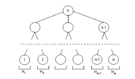
Figure 1: Calculation tree

Only one arc $y_{v}$ comes out from each vertex $v$, $v=1,2,\ldots,k$. It corresponds to a value of the function $\phi_{v}$. We suppose that $y_{v}=X_{v},v=1,2,\ldots,m;y_{k}=\phi=\phi_{k}$.

We denote $I_{v}$ as a set of vertices from which arcs come into the vertex $v$, and $J_{v}$ as a corresponding set of variables (arcs): $i\in I_{v}\Leftrightarrow y_{i}\in J_{v}$. It is clear that $I_{v}=\oslash$ for $v=1,2,\ldots,m$; $y_{v}=f_{v}(J_{v})$, $v=m+1,m+2,\ldots,k$. We suppose that a numbering of the vertices is correct: if $v<w$ than $w\notin I_{v}$.

Now, function value can be calculated by the sweep method. At the beginning, we extract separate elements $X_{1j_{1}(1)},X_{2j_{2}(1)},\ldots,X_{mj_{m}(1)}$ from populations $H_{1},H_{2},\ldots,H_{m}$, then calculate the function values $\phi_{m+1},\phi_{m+2},\ldots$, $\phi_{k}=\phi$ successively. After r such runs the estimator $\Theta^{*}$ is computed according to the formula (2). An analysis of this method was developed in the previous papers of authors.

The Hierarchical Bootstrap method is based on the wave algorithm. Here all values of the function $\phi_{v}$ for each vertex $v=m+1,m+2,\ldots,k$ should be calculated all at once. They form the set $H_{v}=\{Y_{v1},Y_{v2},\ldots,Y_{vn_{v}}\}$, where $n_{v}$ is number of realizations (sample size). Getting one realization $Y_{vl}$ consists of choosing value from each corresponding population $H_{i},i\in I(v)$, and calculation of $\phi_{v}$ value. By this we suppose that a random sample with replacement is used when each element from $H_{i}$ is choosen independendly with the probability $1/n_{i}$. Further on, this procedure is repeated for next vertex. Finally we get $Y_{k1},Y_{k2},\ldots,Y_{kn_{k}}$ as values of the population $H_{k}$. Their average gives the estimator $\Theta^{*}$ by analogy with formula (2).

3 EXPRESSIONS FOR VARIANCE

The aim of this section is to show how to calculate variance $D\;\Theta^{*}$ of the estimator (2). It is easy to see that in the case of Hierarchical Bootstrap the variance $D\;\Theta^{*}$ is function of sample sizes $n_{1},n_{2},\ldots,n_{k}$.

In the previous papers of authors the variance $D\;\Theta^{*}$ was calculated using the $\omega$-pairs notion (Andronov et. al, 1996, 1998). Then, it was considered as continuos function of variables $n_{1},n_{2},\ldots,n_{k}$, and reduced gradient method was used. But now we need other approach for the calculation of $D\;\Theta^{*}$.

We use Taylor decomposition of function $\phi({\bf x})$ in respect to mean ${\bf\mu}=(E\;X_{1},E\;X_{2},\ldots,E\;X_{m})$:

$$\phi({\bf x})=\phi({\bf\mu})+\bigtriangledown^{T}\phi({\bf\mu})({\bf x}-{\bf\mu})+\frac{1}{2}({\bf x}-{\bf\mu})^{T}\bigtriangledown^{2}\phi({\bf\mu})({\bf x}-{\bf\mu})+O(||{\bf x}-{\bf\mu}||^{3}),$$ (3)

where	$\bigtriangledown^{2}\phi({\bf x})$ is the matrix of second derivatives of the function $\phi({\bf x})$,
	$||{\bf v}||$ is Euclidean norm of vector ${\bf v}$.

It gives the following decomposition:

$$\phi({\bf x})\phi({\bf x^{\prime}})= \phi^{2}({\bf\mu})+\phi({\bf\mu})\bigtriangledown^{T}\phi({\bf\mu})({\bf x}-{\bf\mu})+\phi({\bf\mu})\bigtriangledown^{T}\phi({\bf\mu})({\bf x^{\prime}}-{\bf\mu})+$$

$$+\frac{1}{2}\phi({\bf\mu})({\bf x}-{\bf\mu})^{T}\bigtriangledown^{2}\phi({\bf\mu})({\bf x}-{\bf\mu})+$$

$$+\frac{1}{2}\phi({\bf\mu})({\bf x^{\prime}}-{\bf\mu})^{T}\bigtriangledown^{2}\phi({\bf\mu})({\bf x^{\prime}}-{\bf\mu})+$$

$$+\bigtriangledown^{T}\phi({\bf\mu})({\bf x}-{\bf\mu})({\bf x^{\prime}}-{\bf\mu})^{T}\bigtriangledown\phi({\bf\mu})+$$

$$+O(||{\bf x^{\prime}}-{\bf\mu}||^{3}+||{\bf x}-{\bf\mu}||^{3}).$$

If ${\bf X}=(X_{1},X_{2},\ldots,X_{m})$ is a random vector with mutual independent components $\{X_{i}\}$, $E\;{\bf X}={\bf\mu}$, $D\;X_{i}=\sigma^{2}_{i}$, then

$$E\;\phi({\bf X})=\phi({\bf\mu})+\frac{1}{2}\sum_{i=1}^{m}\sigma^{2}_{i}\frac{\partial^{2}}{\partial x_{i}^{2}}\phi({\bf\mu})+E(O(||{\bf X}-{\bf\mu}||^{3})),$$ (5)

$$(E\;\phi({\bf X}))^{2}=\phi^{2}({\bf\mu})+\phi({\bf\mu})\sum_{i=1}^{m}\sigma_{i}^{2}\frac{\partial^{2}}{\partial x_{i}^{2}}\phi({\bf\mu})+\ldots.$$ (6)

Now we suppose that $X_{i}$ and $X^{\prime}_{i}$ are some values from sample population $H_{i}=\{Y_{i1},Y_{i2},\ldots,Y_{in_{i}}\}$. Let $C_{i}$ denote the covariance of two elements $Y_{il}$ and $Y_{il^{\prime}}$ with different numbers $l$ and $l^{\prime}$:

$$C_{i}=Cov(Y_{il},Y_{il^{\prime}}|l\neq l^{\prime}).$$ (7)

Let $X_{i}$ and $X^{\prime}_{i}$ correspond to the elements $Y_{il}$ and $Y_{il^{\prime}}$ accordingly. Because we extract $X_{i}$ and $X_{i}^{\prime}$ from $H_{i}$ at random and with replacement, then the event $\{l\neq l^{\prime}\}$ occurs with the probability $1/n_{i}$. Then

$$Cov(X_{i},X_{i}^{\prime})=\left\{\begin{array}[]{ll}Cov(Y_{il},Y_{il})=D\;Y_{i}&\mbox{with the probability $1/n_{i}$},\\ Cov(Y_{il},Y_{il^{\prime}})=C_{i}&\mbox{with the probability $1-1/n_{i}$}.\end{array}\right.$$ (8)

Therefore

$$Cov(X_{i},X_{i}^{\prime})=\frac{1}{n_{i}}D\;Y_{i}+\left(1-\frac{1}{n_{i}}\right)C_{i}.$$ (9)

If the values $\phi(X)$ and $\phi(X^{\prime})$ correspond to subfunction $y_{v}=\phi_{v}(\cdot)$ and the sample population $H_{v}$, then formulas (3), (5) and (6) give

$$C_{v}=\sum_{i\in I_{v}}\left(\frac{\partial}{\partial x_{i}}\phi_{v}(\mu_{v})\right)^{2}Cov(X_{i},X_{i}^{\prime})+\ldots.$$ (10)

Now we can get from (9)

$$Cov(\phi_{v}(X),\phi_{v}(X^{\prime}))=\frac{1}{n_{v}}\sigma^{2}_{v}+\left(1-\frac{1}{n_{v}}\right)C_{v},$$ (11)

where the variance $\sigma^{2}_{v}=D\;Y_{v}$ can be determined from (10) by $X_{i}=X_{i}^{\prime}$:

$$\sigma^{2}_{v}=\sum_{i\in I_{v}}\left(\frac{\partial}{\partial x_{i}}\phi_{v}(\mu_{v})\right)^{2}\sigma_{i}^{2}+\ldots.$$ (12)

Finally we have

$$Cov(\phi_{v}(X),\phi_{v}(X^{\prime}))=\sum_{i\in I_{v}}\left(\frac{\partial}{\partial x_{i}}\phi_{v}(\mu_{v})\right)^{2}\left[\frac{1}{n_{v}}\sigma_{i}^{2}+\left(1-\frac{1}{n_{v}}\right)Cov(X_{i},X_{i}^{\prime})\right]+\ldots,$$ (13)

or

$$Cov(\phi_{v}(X),\phi_{v}(X^{\prime}))=\sum_{i\in I_{v}}\left(\frac{\partial}{\partial x_{i}}\phi_{v}(\mu_{v})\right)^{2}\left[\left(\frac{1}{n_{v}}+\left(1-\frac{1}{n_{v}}\right)\frac{1}{n_{i}}\right)\sigma^{2}_{i}+\ldots\right.$$

$$\left.+\left(1-\frac{1}{n_{v}}\right)\left(1-\frac{1}{n_{i}}\right)C_{i}\right].$$ (14)

By this we suppose that variances $\sigma_{1}^{2},\sigma_{2}^{2},\ldots,\sigma_{m}^{2}$ of input random variables $X_{1},X_{2},\ldots,X_{m}$ are known. For example, it is possible to use estimators of these variances, calculated on given sample populations $H_{1},H_{2},\ldots,H_{m}$.

If the vertex $i$ belongs to the initial level of the calculation tree (it means that $i=1,2,\ldots,m$) then $\phi_{i}(x_{i})=x_{i}$, $\sigma_{i}^{2}$ is known value, $C_{i}=0$. Therefore

$$Cov(\phi_{i}(X_{i}),\phi_{i}(X^{\prime}_{i}))=\frac{1}{n_{i}}\sigma_{i}^{2},\qquad i=1,2,\ldots,m.$$ (15)

Another covariances and variances are calculated recurrently in accordance with formulas (10),(12), (14), (15) from vertices with less numbers to vertices with great numbers. Finally we get the variance $D\;\Theta^{*}$ of interest as the variance for root of the calculation tree:

$$D\;\Theta^{*}=\frac{1}{r}(\sigma_{k}^{2}+(r-1)C_{k})+\ldots,$$ (16)

where $r=n_{k}$.

As it was just mentioned, we will consider the variance $D\;\Theta^{*}$ as a function of sample sizes $n_{1},n_{2},\ldots,n_{k}$ and denote it $D(n_{1},n_{2},\ldots,n_{k})$. Our aim is to minimize this function in respect to variables $n_{1},n_{2},\ldots,n_{k}$ by linear restriction, or, by other words, to solve the following optimization problem:

$$\mbox{minimize }D(n_{1},n_{2},\ldots,n_{k})$$ (17)

by restriction

$$a_{1}n_{1}+a_{2}n_{2}+\ldots+a_{k}n_{k}\leq b,$$ (18)

where $b$, $\{a_{i}\}$ and $\{n_{i}\}$ are integer non-negative numbers.

Now we intent to apply the dynamic programming method (Minox 1989).

4 THE DYNAMIC PROGRAMMING METHOD

Let us solve the optimization problem (17), (18). Our function of interest $\phi({\bf x})$ is calculated and simulated recurrently, using the calculation tree (see Section 2). In accordance to the dynamic programming technique, we have ”forward” and ”backward” procedure.

During ”backward” procedure, we calculate recurrently so-called Bellman function $\Phi_{v}(\alpha,z)$, $v=1,2,\ldots,k$, $z=1,2,\ldots,b$, $0\leq\alpha\leq 1$. Let us consider the subfunction $\phi_{v}(\cdot)$, that corresponds to the vertex $v$. This subfunction directly depends on variables $y_{i}$, $i\in I_{v}$, which correspond to incoming arcs for the vertex $v$. Additionally $\phi_{v}$ depends on variables $\{x_{i}\}$ and $\{y_{i}\}$ from which there exists path from leaves to the vertex $v$ of our calculation tree. Let $B_{v}$ denote corresponding set of variables $\{x_{i}\}$ and $\{y_{i}\}$.

Now we need to denote some auxiliary functions. Let us introduce the following notation

$$\psi_{i}(\alpha)=\alpha\sigma_{i}^{2}+(1-\alpha)Cov(X_{i},X^{\prime}_{i}),\qquad i=1,2,\ldots,k,\;0\leq\alpha\leq 1.$$ (19)

Then we are able to write in accordance with (13):

$$Cov(\phi_{v}(X),\phi_{v}(X^{\prime}))=\sum_{i\in I_{v}}\left(\frac{\partial}{\partial x_{i}}\phi_{v}(\mu_{v})\right)^{2}\psi_{i}\left(\frac{1}{n_{v}}\right).$$ (20)

Now we have from (19), (12) and (13)

$$\psi_{v}(\alpha)=\sum_{i\in I_{v}}\left(\frac{\partial}{\partial x_{i}}\phi_{v}(\mu_{v})\right)^{2}\left\{\alpha\sigma_{i}^{2}+(1-\alpha)\left[\frac{1}{n_{v}}\sigma_{i}^{2}+(1-\frac{1}{n_{v}})Cov(X_{i},X_{i}^{\prime})\right]\right\}=$$

$$\sum_{i\in I_{v}}\left(\frac{\partial}{\partial x_{i}}\phi_{v}(\mu_{v})\right)^{2}\left[\left(\alpha+\frac{1-\alpha}{n_{v}}\right)\sigma_{i}^{2}+(1-\alpha)(1-\frac{1}{n_{v}})Cov(X_{i},X^{\prime}_{i})\right],$$

so

$$\psi_{v}(\alpha)=\sum_{i\in I_{v}}\left(\frac{\partial}{\partial x_{i}}\phi_{v}(\mu_{v})\right)^{2}\psi_{i}\left(\alpha+\frac{1-\alpha}{n_{v}}\right).$$ (21)

Note that it follows from (11) and (19) that our variance of interest (16) is

$$D\;\Theta^{*}=\psi_{k}(0).$$ (22)

Values $\psi_{v}(\alpha)$ depend on the sample sizes $n_{i}$ for all $i\in B_{v}$. We will mark this fact as $\psi_{v}(\alpha)=\psi_{v}(\alpha;n_{i}:i\in B_{v})$.

Now we are able to introduce above mentioned Bellman functions:

$$\Phi_{v}(\alpha,z)=\min_{n_{i}}\psi_{v}(\alpha;n_{i}:i\in B_{v}),$$ (23)

where minimization is realized with respect to non-negative integer variables $n_{i}$ that are satisfied the linear restriction

$$\sum_{i\in B_{v}}a_{i}n_{i}\leq z.$$ (24)

It is clear that optimal value of variance $D^{*}(\cdot)$ for the problem (17), (18) is equal to $\Phi_{k}(0,b)$.

Bellman functions $\Phi_{v}(\alpha,z)$ are calculated recurrently from $v=1$ to $v=k$ for $0\leq\alpha\leq 1$ and $z=1,2,\ldots,b$. Basic functional equation of dynamic programming has the following form:

$$\Phi_{v}(\alpha,z)=\min\sum_{i\in I_{v}}\left(\frac{\partial}{\partial x_{i}}\phi_{v}(\mu_{v})\right)^{2}\Phi_{i}\left(\alpha+\frac{1-\alpha}{n_{v}};z_{i}\right)$$ (25)

where minimaiztion is realized with respect to non-negative integer variables $n_{v}$ and $\{z_{i}:i\in I_{v}\}$ that satisfy the linear restriction

$$a_{v}n_{v}+\sum_{i\in I_{v}}z_{i}\leq z.$$ (26)

The initial values of $\Phi_{v}(\cdot)$ are determined with the tree leaves by formulas (15), (19) and (23):

$$\Phi_{v}(\alpha,z)=\alpha\sigma^{2}_{v}+(1-\alpha)\frac{1}{[z/a_{v}]}\sigma_{v}^{2}=$$ (27)

$$=\sigma_{v}^{2}\left(\alpha+(1-\alpha)\frac{1}{[z/a_{v}]}\right),\qquad v=1,2,\ldots,m,$$

where $[z/a_{v}]$ - integer part of number $z/a_{v}$,

Thus the ”backward” procedure is a recurrent calculation of Bellman functions $\Phi_{v}(\alpha,z)$ for $v=1,2,\ldots,k$, $0\leq\alpha\leq 1$, $z=1,2,\ldots,b$ by using formulas (27), (25). Finally we get the minimal variance

$$D^{*}\;\Theta^{*}=\Phi_{k}(0,b).$$ (28)

To calculate the optimal sample sizes $n^{*}_{1},n^{*}_{2},\ldots,n^{*}_{k}$ we should apply ”forward” procedure of dynamic programming technique. At first, we find $n^{*}_{k}$ and $\{z^{*}_{i}:i\in I_{k}\}$ by solving the equation

$$\Phi_{k}(0,b)=\min\sum_{i\in I_{k}}\left(\frac{\partial}{\partial x_{i}}\phi_{k}(\mu_{k})\right)^{2}\Phi_{i}\left(\frac{1}{n^{*}_{k}},z_{i}^{*}\right)$$ (29)

where minimization is realized by condition

$$a_{k}n_{k}^{*}+\sum_{i\in I_{k}}z_{i}^{*}\leq b.$$ (30)

Let $I^{-1}(v)=\{\omega:v\in I(\omega)\}$, $\alpha_{k}=1/n_{k}^{*}$. Then we recurrently determine by analogy the rest $n_{v}^{*}$ and $\{z^{*}_{i}:i\in I_{v}\}$ for $v=k-1,k-2,\ldots,m+1$:

$$\Phi_{v}(\alpha_{I^{-1}(v)},z^{*}_{v})=\min\sum_{i\in I_{v}}\left(\frac{\partial}{\partial x_{i}}\phi_{v}(\mu_{v})\right)^{2}\Phi_{i}\left(\alpha_{I^{-1}(v)}+\frac{1-\alpha_{I^{-1}(v)}}{n_{v}^{*}},z_{i}^{*}\right)$$ (31)

by condition

$$a_{v}n_{v}^{*}+\sum_{i\in I_{v}}z_{i}^{*}\leq z_{v}^{*}.$$ (32)

Moreover we put

$$\alpha_{v}=\alpha_{I^{-1}(v)}+(1-\alpha_{I^{-1}(v)})/n_{v}^{*}$$ (33)

Finally the optimal sizes $n_{i}^{*}$ for $i=1,2,\ldots,m$ are determined by the following way:

$$n_{i}^{*}=[z_{i}^{*}/a_{i}].$$ (34)

References

Andronov, A., Merkuryev, Yu. (1996) Optimization of Statistical Sizes in Simulation. In: Proceedings of the 2-nd St. Petersburg Workshop on Simulation, St. Petersburg State University, St. Petersburg, 220-225.

Andronov, A., Merkuryev, Yu. (1998) Controlled Bootstrap Method and its Application in Simulation of Hierarchical Structures. In: Proceedings of the 3-d St. Petersburg Workshop on Simulation, St. Petersburg State University, St. Petersburg, 271-277.

Davison, A.C., Hinkley, D.V. (1997) Bootstrap Methods and their Application. Cambridge university Press, Cambridge.

Efron, B., Tibshirani, R.Y. (1993) Introduction to the Bootstrap. Chapman & Hall, London.

Minox, M. (1989) Programmation Mathematique. Teorie et Algorithmes. Dunod.