Optimizing Vetoes for Gravitational-wave Transient Searches

Abstract

Interferometric gravitational-wave detectors like LIGO, GEO600 and Virgo record a surplus of information above and beyond possible gravitational-wave events. These auxiliary channels capture information about the state of the detector and its surroundings which can be used to infer potential terrestrial noise sources of some gravitational-wave-like events. We present an algorithm addressing the ordering (or equivalently optimizing) of such information from auxiliary systems in gravitational-wave detectors to establish veto conditions in searches for gravitational-wave transients. The procedure was used to identify vetoes for searches for unmodeled transients by the LIGO and Virgo collaborations during their science runs from 2005 through 2007. In this work we present the details of the algorithm; we also use a limited amount of data from LIGO’s past runs in order to examine the method, compare it with other methods, and identify its potential to characterize the instruments themselves. We examine the dependence of Receiver Operating Characteristic curves on the various parameters of the veto method and the implementation on real data. We find that the method robustly determines important auxiliary channels, ordering them by the apparent strength of their correlations to the gravitational-wave channel. This list can substantially reduce the background of noise events in the gravitational-wave data. In this way it can identify the source of glitches in the detector as well as assist in establishing confidence in the detection of gravitational-wave transients.

Keywords: Gravitational waves, Interferometric detectors, LIGO, Virgo, Vetoes, Auxilliary Channels, Statistical Methods

1 Introduction

The Laser Interferometer Gravitational-wave Observatory (LIGO) [1] together with Virgo [2] and GEO600 [3] form a network of detectors employing kilometer-scale interferometers to search for gravitational waves (GWs) from astrophysical and cosmological sources. One such class of sources is expected to result in short-lived signals lasting from milliseconds to several seconds within the sensitive frequency band of the instruments. They may correspond to core-collapse supernovae, neutron star glitches, cosmic string cusps and kinks, magnetars or some binary compact systems (made up of neutron stars/black holes) [4]. Environmental and instrumental noise sources may generate similar short-lived signals through their coupling to the GW sensing channel. These signals are colloquially referred to as “glitches.” During the first-generation instruments’ operation (2002-2010), such glitches were non-Gaussian and non-stationary and presented challenges when searching for transients of astrophysical origin. For well modeled GW transient sources (like most of the binary compact star coalescences), knowledge of the expected signal waveform significantly helps reject such glitches. These signal-based vetoes have been developed and invoked in existing searches [5, 6]. However, for unmodeled (or poorly modeled) transient searches, such glitches may drive detection thresholds to significantly higher values than one would expect for Gaussian backgrounds [7, 8].

Interferometric detectors record their physical environment and detailed interferometry status through thousands of auxiliary channels that present no or negligible coupling to GWs. Information from these channels presents an important handle for understanding (and fixing) the sources of noise in the instruments, reducing the background and ultimately establishing confidence in detections. The problem of identifying and “mechanizing” the use of information from auxiliary channels is long standing within the GW data analysis community [9, 10, 11].

A number of statistical quantities have been developed [12] in order to help characterize the performance of a particular auxiliary channel or veto strategy, such as veto efficiency: the fraction of GW-channel glitches removed, use percentage: the fraction of auxiliary channel glitches which can be associated with a GW-channel glitch [9, 13], dead-time: the effective fraction of analysis live-time removed when applying the veto strategy, and veto significance: the statistical significance of a measured correlation between auxiliary and GW-channel glitches assuming random coincidence [14]. These veto metrics are most appropriate for a simple veto strategy, such as a coincidence between the auxiliary and GW-channel glitch within a short specified time window. Expansions on this approach include making use of our knowledge of the instrument to anticipate when noise coupling between the auxiliary and GW channels is strongest and/or consistent with observation [15, 16]. The use of machine learning algorithms to digest the large amounts of auxiliary channel information and predict GW-channel glitches is also an active area of study [17]. Aside from auxiliary information, signal consistency of the event across multiple instruments, or between the observed signal and theoretical waveform, provide an extremely powerful way to reject noise transients. However, accidental transient noise coincidence across multiple instruments is still a dominant source of background in astrophysical searches, especially in searches for unmodeled transients.

In this paper we present an algorithm which we will call Ordered Veto List (OVL). It exploits the information from the auxiliary channels in GW detectors and uses a unified ranking metric, veto efficiency divided by dead-time (described earlier), in order to make inferences about the source of GW-channel events recorded at each detector. The OVL algorithm operates by generating a small time window surrounding a glitch in an auxiliary channel. If a GW-channel transient is present within this window, it is assumed to be noise and removed. An earlier version of the method, described in [18], was used to identify noise transients in a search for GW bursts during LIGO’s fifth and Virgo’s first science runs [19, 7].

OVL addresses several problems with the simple strategy of removing all live-time associated with a disturbance in an auxiliary channel. First, OVL identifies only those channels with noise that couples in a statistically significant way to the GW channel, thus avoiding the unnecessary removal of live-time. Second, when multiple auxiliary channels cover the same transient disturbances in the instrument, OVL selects the channel which optimally removes background with minimal loss of live-time. Ultimately, OVL provides an ordered list of rules to follow for successively removing time from the analysis based on auxiliary channel information, with the most effective channels at the top of the list [14]. The ordered list also provides a metric representing our confidence that any particular event is instrumental in origin.

Another hierarchical veto selection method, h-veto [20], has been developed. Both methods have a similar strategy for ranking veto channels. The major difference is in the figure-of-merit used in the ordering process. The ranking for h-veto depends on the statistical significance of the correlation between the auxiliary and GW channels under the assumption of a Poisson process. This choice favors large statistics, and generally results in a short list of highly-efficient vetoes, where each entry represents the most relevant physical parameters (e.g. time-scale) of the coupling. OVL, on the other hand, ranks vetoes by the ratio of efficiency divided by the fractional dead-time. This favors vetoes which have the highest rate of GW-channel transients within their chosen exclusion windows. In this ranking, it is common for the same auxiliary channel to appear multiple times in the list with different thresholds on glitch strength or different exclusion window durations. Typically a channel is chosen first at the highest thresholds (strongest auxiliary channel disturbances) and smallest exclusion windows, and only appears later with more relaxed parameters. This choice maximizes the overall efficiency obtained using the best veto parameters at a fixed dead-time threshold at the expense of a longer, interlaced list which can be more difficult to interpret. Finally, in OVL, the veto windows are explicitly calculated as a set of non-overlapping time intervals (segments), and overlaps between different veto conditions are calculated exactly. This can be important when considering highly-correlated auxiliary channels with significant overlap.

This paper is organized as follows. In Section 2, we describe the OVL algorithm, including construction of veto configurations and their application to GW-channel data. In Section 3, we discuss OVL’s performance when applied to two samples of LIGO data: one month from LIGO’s fourth science run (S4) and one week from LIGO’s sixth science run (S6). We evaluate the method’s performance using Receiver Operating Characteristic (ROC) curves and examine some features of the ordering generated. We conclude in Section 5.

2 Description of the algorithm

OVL is based on a simple process, which includes constructing veto-configurations, the application of those configurations to GW-channel data, and iteration. It uses glitches identified by a generic transient-finding algorithm called Kleine Welle (KW) [21]. Each of these glitches is characterized by a time, duration, frequency content, and significance. While all our investigations are based on KW, any glitch-finding method able to provide at least a time and a significance for each event can be used. In this way, OVL can be adapted to specific searches for different types of GW signals, or to more general detection problems beyond GW astronomy.

2.1 Construction of veto configurations

The OVL algorithm systematically searches for coincident signals in the GW and auxiliary channels by identifying glitches in the GW channel that fall within pre-defined time-window surrounding glitches in an auxiliary channel. In order to accommodate the variety of possible couplings between auxiliary channels and the GW channel, the algorithm tries a variety of window sizes and thresholds on auxiliary glitch thresholds. Each configuration is labeled by a set of three parameters: auxiliary channel name, a threshold on the significance of auxiliary glitches, and time window. OVL uses all permutations of auxiliary channels, significance-thresholds and time-windows to create a diverse set of configurations. In the specified auxiliary channel, OVL selects only those glitches with significance above the threshold, and then time-windows are constructed around the central time of each remaining glitch. The union of these time windows forms a list of (possibly) disjoint segments that are used to remove livetime. Figure 1 demonstrates this procedure using some artificial data.

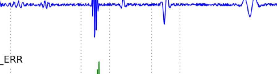
Figure 1: A cartoon showing how veto segments are constructed for a given configuration. Time runs on the x-axis while the y-axis is an arbitrary quantity that may represent the amplitude of the signal in the time-domain or some scalar quantity reflecting its significance in a time-frequency decomposition. In an auxiliary channel (labeled “vchan” here), a threshold is applied to the glitches (shown as “vthr”) and then windows (indicated as “vwin” above) are created surrounding those glitches. The union of these windows is then used to remove time from the GW channel (shown as “DARM_ERR” above), thereby vetoing some GW-channel glitches.

The algorithm creates these configurations to separate and categorize different types of auxiliary glitches. It then applies the configurations to the GW-channel data and searches for an optimal order. This allows the method to find highly correlated configurations while removing spurious information from uncorrelated channels, thereby identifying troublesome auxiliary channels or glitches.

There is no reason the parameters describing each configuration must be limited to channel name, time-window, and significance threshold. By including other degrees of freedom such as frequency bands, glitch duration, data epoch, or time of day (e.g. mornings vs. evenings), the algorithm will be able to find more specific correlations between configurations and GW-channel data, giving better overall performance. However, the total number of configurations must also be balanced against the number of auxiliary glitches available in order to maintain sufficient statistics.

2.2 Initial application of veto configurations to GW-channel data

OVL is based on the idea of ordering veto configurations by their correlations with GW-channel data. We achieve this by associating a figure-of-merit with each veto configuration. Initially, we assume there is no way to know which configuration will perform well, and we give each an equal opportunity. Each veto configuration is applied to the entire GW-channel data set, which we represent as a list of times corresponding to GW-channel glitches. For each veto configuration, veto-segements are generated as prescribed in Section 2.1. We then count the number of GW-channel glitches that fall within these segments, and determine the configuration’s efficiency, the fraction of events removed. Likewise, we determine the fractional dead-time for the configuration by measuring the fraction of livetime contained in the veto segments using explicit segment arithmetic. The ratio of these two quantities defines OVL’s figure-of-merit, which we will refer to as efficiency-over-dead-time. This “base-line” efficiency-over-dead-time measurement is then used to find an initial ordering scheme for all veto configurations. Figure 1 shows how this looks when comparing two time series.

We should note that the efficiency-over-dead-time has a straightforward interpretation in terms of Poisson processes. We can write the efficiency as $\varepsilon=n_{c}/N_{GW}$ and fractional dead-time as $f=t/T$ where $n_{c}$ is the observed number of coincident events, $N_{GW}$ is the total number of GW-channel glitches, $t$ is the amount of time contained in the veto-segments and $T$ is the total amount of live-time. We then have

$$\varepsilon/f=\frac{n_{c}}{t(N_{GW}/T)}\approx\frac{n_{c}}{t\lambda_{GW}}$$ (1)

where $\lambda_{GW}$ is an estimate of the rate of GW-channel glitches. This means that $t\lambda_{GW}\approx\left<n_{c}\right>$, the expected number of GW-channel coincidences that will randomly fall within the veto-segments. We then see that the efficiency-over-dead-time is nothing but the ratio of the observed coincident events to the expected number of coincident events. As we will see in the results and analysis section, we observe efficiency-over-dead-times as high as $10^{4}$ for some highly-correlated configurations.

Besides associating an efficiency-over-dead-time with each configuration, OVL also records the Poisson significance of finding the measured number of coincidences. We compute the Poisson significance as the cumulative probability of observing as many or more coincident GW-channel glitches given the expected number of coincident glitches. OVL uses this significance threshold to avoid over-training by requiring the observed correlations to be reasonably unlikely to occur by chance given the large number of configurations tested.

We should note that rankings based on efficiency-over-dead-time and rankings based on Poisson-significance (as is done with h-veto) are not equivalent, and the two metrics may generate different lists. We can see this by noting that the statistical significance of observing a given number of coincidences can be written as

$$p=\sum_{k=n_{c}}^{\infty}\frac{\left<n_{c}\right>^{k}}{k!}e^{-\left<n_{c}\right>}=\sum_{k=n_{c}}^{\infty}\frac{\left(n_{c}(f/\varepsilon)\right)^{k}}{k!}e^{-n_{c}(f/\varepsilon)}.$$ (2)

We then see that the statistical significance is a function of both the number of coincident events and efficiency-over-dead-time. Generally, for a given $\varepsilon/f$, the Poisson statistical significance will favor veto configurations with large $n_{c}$, and therefore favors configurations with large number statistics versus a ranking based only on $\varepsilon/f$.

2.3 Iteration and ordering

Once a “base-line” efficiency-over-deadtime has been determined for each veto configuration, they are ordered accordingly. At this point, veto configurations are applied hierarchically. When a configuration is applied, OVL counts the number of coincident GW-channel glitches and evaluates the associated efficiency-over-deadtime and Poisson-significance. The GW-channel glitches and veto-segments associated with this configuration are removed from the rest of the analysis. In this way, OVL prevents redundant vetoes. Later configurations do not count GW-channel events or live-time already removed by previous configurations. This data-reduction scheme is applied after each configuration, and therefore each veto configuration in the list sees a slightly different set of GW-channel glitches. Furthermore, the statistics computed for each configuration do not represent global fractions, but rather are fractions of a subset of data. This also allows OVL to measure the additional information contained in later configurations. If they are completely redundant with an earlier configuration, then they will not find any new GW-channel glitches and their efficiency-over-deadtime will vanish. In this way, OVL can remove spurious, extraneous, or redundant veto configurations.

This begs the question of what determines an important configuration. We define these as configurations that yield both a sufficiently high efficiency-over-deadtime and Poisson-significance. Because these are functionally dependent, we can think of this as requiring a sufficient strength of correlation and a sufficiently large number of observed coincidences. By including the Poisson-significance threshold, OVL tends to reject extremely low number statistics with low correlation strength, which makes the ordered list’s performance more robust when applying it to different data sets. If configurations do not perform above these two thresholds, they are removed from the list. This process helps OVL to converge rapidly, and prevents under-performing channels which will be removed in the next iteration from affecting the performance of later channels. For final evaluation of a list’s performance after the ordering process is complete, all channels in the list are applied.

In practice, the entire method is repeated several times, which allows for repeated evaluation and ranking of the configurations. After each iteration, the veto configurations are re-ordered according to their most recent efficiency–over–dead-time measurements. The next iteration re-applied the configurations in this new order. If that order is optimal, it won’t change between iterations. After about 2 iterations, the list gains the bulk of its performance, with a nearly monotonic decrease in efficiency-over-dead-time as one reads down the ordered list. The near monotonicity is caused by the finite number of iterations, as well as phenomena analogous to cycles in Markov processes. Once a sufficiently monotonic list is created, further iterations do not have a large impact on performance, but they can help simplify the list by removing unnecessary configurations, and are relatively cheap to calculate because the final lists are comparatively short.

3 Results and analysis

An earlier version of this method [18] was used to reject transient noise artifacts in searches for unmodeled bursts in LIGO’s fifth science run (S5) and Virgo’s first science run (VSR1) data [19, 7]. In those searches, the method was able to reject 13–45% of single-detector glitches and 5–10% of coincident background (which is generally weak) at under 1% dead-time. In order to further study the performance and systematics of the OVL procedure, we analysed the entirety of LIGO S4 data (February 22, 2005 - March 25, 2005) from the LIGO Hanford Observatory (H1) and one week of LIGO S6 data (May 28, 2010 - June 4, 2010) from the LIGO Livingston Observatory (L1) using KW glitches [21]. These two data sets were collected from geographically distant detectors and are separated by several years. They therefore represent very different noise environments. Furthermore, because the LIGO detectors underwent significant commissioning between S4 and S6, these data sets may capture different couplings between auxiliary channels and the GW-channel data. Therefore, the similarities in OVL’s performance on these very different data sets allows us to draw conclusions about the method rather than peculiarities in either data set.

In this analysis, because there may be causal relations between the GW-channel and auxiliary channels, we restrict ourselves to a subset of auxiliary channels shown to be minimally coupled to the GW channel and thus safe to be used as vetoes. These safety relations are determined through hardware injections at the sites, in which the test masses are driven with a known GW-like transient waveform. Searches for these transients in auxiliary channels during hardware injections at the instruments have been used to establish the exact conditions on their strength (either absolute or related to the GW-channel signal) that make them “safe”, i.e., ensuring that they will not systematically reject an astrophysical GW transient [22, 19, 8].

In what follows, we find similar performance between the two data sets, and describe the characteristics of the method. In both cases, OVL identifies a subset of channels that appear to be correlated with the GW-channel data which is significantly smaller than the set of all auxiliary channels.

Our implementation of this algorithm used python. An AMD 2.7 GHz 32-bit processor processed $3.7\times 10^{4}$ seconds of data containing $2.8\times 10^{3}$ GW-channel glitches with 250 auxiliary channels from S6 in approximately 9 hours. Nearly half the computational effort is spent on the first two iterations, with the following iterations processing much faster.

3.1 ROC curves and bulk statistics

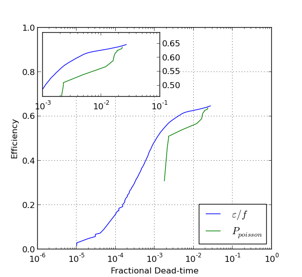
Figure 2: Comparison of ranking by two figures of merit. Both curves are generated over the S6 data set, using the same code, set of configurations, and performance thresholds. These curves represent the 9^th iteration through OVL, when both ordered lists have settled down to a near optimal order. We see that the efficiency-over-deadtime ($\varepsilon/f$: blue) curve is better than the Poisson Significance curve ($P_{poisson}$: green)). Efficiency–over-dead-time also produces a much smoother curve, indicating that Poisson significance favors larger-number statistics.

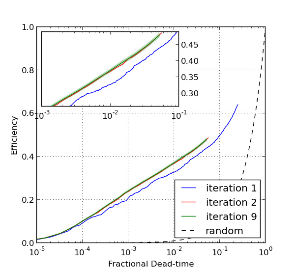
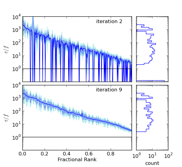
(a) S4 H1

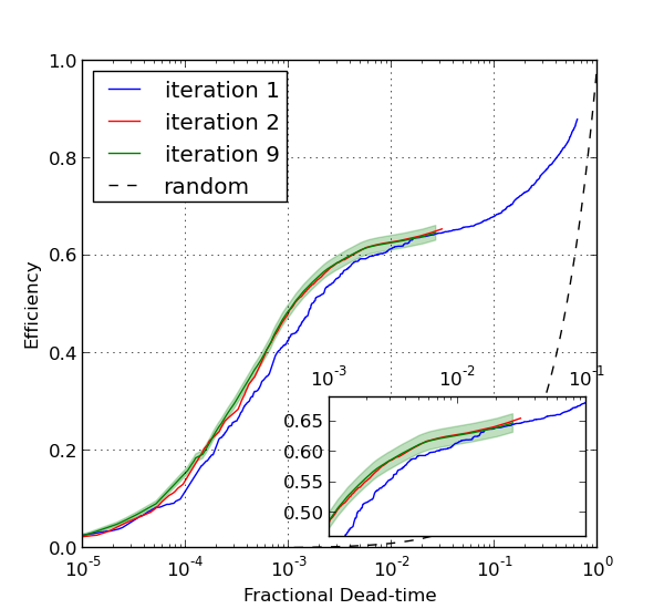
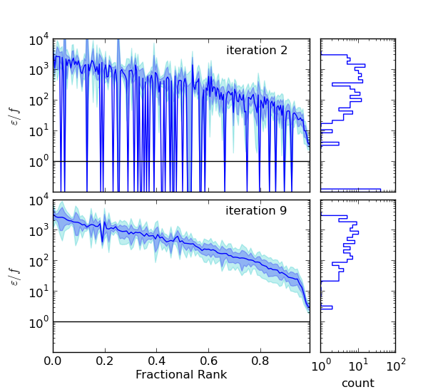
(b) S6 L1

Figure 3: (Left) Receiver Operating Characteristic curves. These plots show OVL’s performance after different numbers of iterations. Importantly, iteration 1 represents the ordering generated by applying individual veto configurations independently to the entire data set. We would expect the algorithm to improve with further iteration because it can better order its list of vetoes, but we see that the bulk efficiency gains are achieved after only two iterations. There are marginal gains with further iterations, but these are well within the expected errors. The shaded regions represent 68% confidence intervals. (Right) The relation between OVL’s figure of merit ($\varepsilon/f=$ efficiency-over-deadtime) and the veto-configuration’s order in the list for S4 and S6 data. We expect a nearly monotonic decrease for well-trained lists. The blue curve denotes the point-estimate, with the shaded regions representing 68% and 95% confidence intervals. We see that the errors are relatively small in these plots, in contrast to Figure 4 where the same analysis is repeated for uncorrelated data. There is the additional feature in the S6 data: a distinct knee in these plots at high fractional rank. This suggests a large special population of easily-vetoed glitches. The projected histograms show the grouping of $\varepsilon/f$, with the peak clearly above Poisson coincidence’s prediction of 1. The bin with $\varepsilon/f=0$ corresponds to configurations that do not find any coincident GW-channel events.

The Receiver Operating Characteristic (ROC) curve is the basic diagnostic for how the OVL algorithm performs. It shows the fraction of GW-channel glitches removed as a function of the fraction of live-time removed. As a first experiment, we compared two ranking figures-of-merit: efficiency-over-deadtime and the Poisson significance, both described in Section 2.2. Figure 2 shows the ROC curves for each ranking scheme. As expected, ranking by incremental efficiency-over-deadtime results in a higher-performing ROC when measuring overall cumulative efficiency as a function of dead-time, though the two rankings begin to converge near at the end where all effective veto conditions are used up. Furthermore, the Poisson significance selects many fewer configurations, each covering a larger number of events. This is seen clearly by the discreteness of the curve. A short veto list is often convenient for simplicity and ease of interpretation. A smooth curve with many configurations may also be preferable in cases where one requires a continuous ranking parameter.

As stated above, OVL’s performance improves upon iteration, but the majority of the efficiency gains are achieved after 2 iterations. Figure 3 shows OVL’s performance after several different iterations. The main advantage of running to 9 iterations is a reduction in the number of veto configurations identified. Table 1 shows that the number of important channels stabilizes rather early, but the number of important configurations continues to decrease. This means that further iteration helps to compress the information stored in the important channels into a shorter list and determine exactly which glitches in which channels are most troublesome.

Table 1: Number of auxiliary channels and veto-configurations present in OVL as a function of iteration number. We see that the number of important channels stabilizes quickly and corresponds to the bulk efficiency gains seen in Figure 3. The information in these channels is then compressed into a small number of veto-configurations (corresponding to different values of auxiliary channel glitch significance and coincidence time-window) upon further iterations.

iteration		initial	1	2	3	4	5	6	7	8	9
S4 H1	No. chan	161	106	99	52	47	47	47	47	47	47
	No. config	7245	3117	294	196	183	178	176	176	176	175
S6 L1	No. chan	202	44	37	35	35	35	35	35	35	35
	No. config	11250	4361	209	140	128	119	118	118	117	117

We also note that the ordering improves upon further iteration. Figure 3 shows the relation between a configuration’s efficiency-over-deadtime and its position in the list for different iterations. We observe a general smoothing with further iterations. Even though the bulk of OVL’s performance is gained after 2 iterations, the list still contains many irrelevant and underperforming configurations. By iteration 9, these configurations have been removed and efficiency-over-deadtime decrease much more smoothly, although there are still some fluctuations. Furthermore, the histograms of efficiency-over-deadtime show the distribution of performance over the list. We see that the peak of the distribution is well away from the Poisson coincidence prediction of 1, and iteration does not damage this distribution.

3.2 Performance on uncorrelated data

In order to further check the overall implementation and performance of our veto algorithm, we examined its output when it was applied on uncorrelated data. For this purpose we constructed artificial data sets by randomly shifting the auxiliary glitches in every channel by a different amount of time using S6 data. In this way, we break all temporal correlations between the GW channel and auxiliary channels, as well as between the auxiliary channels themselves. We therefore expect OVL to be subject only to correlations due to statistical fluctuations in the coincidence of two Poisson processes. We processed this data through the OVL pipeline and examined the ROC curve as well as the dependence of the algorithm’s figure of merit as a function of a configuration’s fractional rank. This is shown in Figure 4.

When compared with the plots in Figure 3 we see that the ROC curve is much worse for the uncorrelated data, as expected. However, there are common features in the lists, namely the comparable decay in efficiency-over-deadtime as one moves to higher ranks.

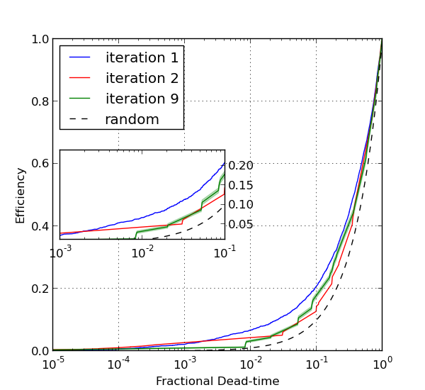
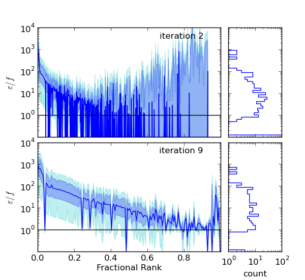
Figure 4: (Left) Receiver Operating Characteristic curves for uncorrelated data. We see that the ROC curves are much worse than those for correlated data. (Right) The relation between OVL’s figure of merit and the veto-configuration’s order in the list for time-shifted S6 data. The bin with $\varepsilon/f=0$ corresponds to configurations that do not find any coincident GW-channel events. We see that there is still the general trend seen in Figure 3, however the errors are somewhat larger here. This is most noticeable because the upper error estimates are significantly higher in this figure. This is expected, because all coincident GW-channel glitches are due to pure chance in the time-shifted data, and the errors are dominated by small number statistics and the lower bound $n_{c}\geq 0$.

Figure 4 shows the relation between efficiency-over-deadtime and a configuration’s rank. This ordering consists of over-training only because it represents OVL’s performance when evaluated on the same data used to generate the ordered list. We should note that when we apply the threshold on Poisson significance used for the correlated data to this uncorrelated data, only $1\%$ of these configuration survive. However, by lowering the Poisson significance threshold, we are able to examine the underlying distribution of noise in our analysis. We can immediately interpret our threshold on efficiency-over-deadtime from the projected histogram as designed to separate the distributions for correlated data (Figure 3) and uncorrelated data (Figure 4).

3.3 Round robin algorithm

There exists a potential danger of over-training OVL with a single data set, which may produce artificially high performance that will not generalize to other data. For this purpose, we performed a simple cross-referencing procedure that shows this is not significant for our results. We divided the data into separate sets, which were arranged like a 1-dimensional checker-board in time, meaning the $k^{\mathrm{th}}$ bin contains every $k^{\mathrm{th}}$ minute of the livetime. Training was then performed on all sets except one, and that one set was used for evaluation. This was carried out with each set, so we have a measure of the algorithm’s performance over all our data. Fig 5 shows a comparison between the round robin and non-round robin procedure. We see that there is no significant difference between the two curves at the 68% confidence level, although there is a small systematic error introduced. The consistency between round robin and non-round robin performance is due to OVL’s threshold on Poisson significance, described in Section 2.2. By requiring the number of observed coincidences to be statistically significant relative to the total number of veto configurations tested, OVL can reject configurations with low number statistics that may pass the performance threshold due to random coincidence alone.

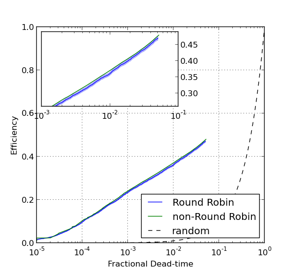
(a) S4 H1

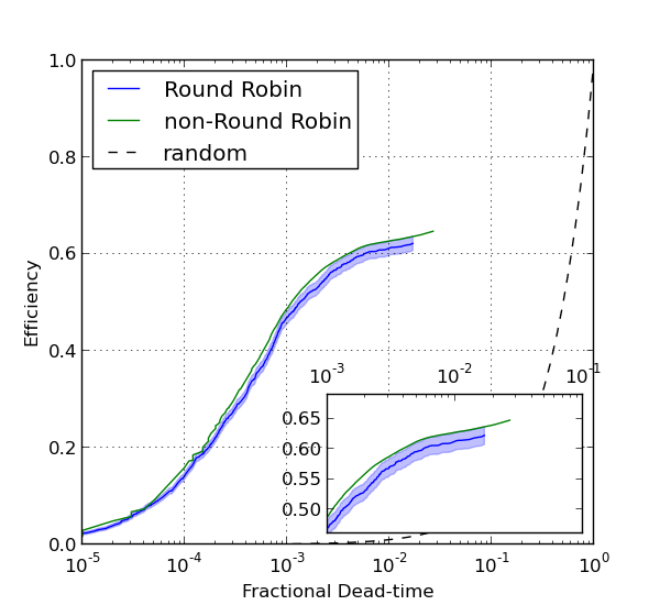
(b) S6 L1

Figure 5: A comparison of round robin and non-round robin analysis techniques. Shaded regions represent 68% confidence intervals. The round robin algorithm ensures that lists are developed and then evaluated using disjoint data sets. However, we see that the application to disjoint data has a very small affect on the list’s performance. This suggests that OVL finds overwhelmingly true correlations in the data. The observed decrease in performance could be due to a combination small over-training errors as well as statistical fluctuations caused by evaluating a list’s performance on a smaller data set (implicit in the division associated with round robin analysis).

We also examine the performance of individual configurations when round robin binning is used. Figure 6 shows the efficiency-over-deadtime for correlated and uncorrelated S6 data (discussed further in Section 3.2), and should be compared with Figures 3 and 4. It is clear that both correlated and uncorrelated data contain some configurations that do not perform well on disjoint data. These are likely due to statistical fluctuations and represent the sharp spikes in these plots. However, we also see that consistent performance is the norm in correlated data, whereas under-performance is the norm for uncorrelated data. The few outliers in the uncorrelated data set are due to single auxiliary glitches that happen to coincide with GW-channel events, and are statistical in nature. We also note that the distributions over efficiency-over-deadtime are very different for the two data sets. Encouragingly, the uncorrelated data appears to have a peak in likelihood near $\varepsilon/f=1$, which agrees with our Poissonian interpretation. We should also note that the ordering in the uncorrelated data is generated entirely by statistical errors in the estimation of efficiency and dead-time, which is clearly visible in the error estimates for uncorrelated data show in Figure 6.

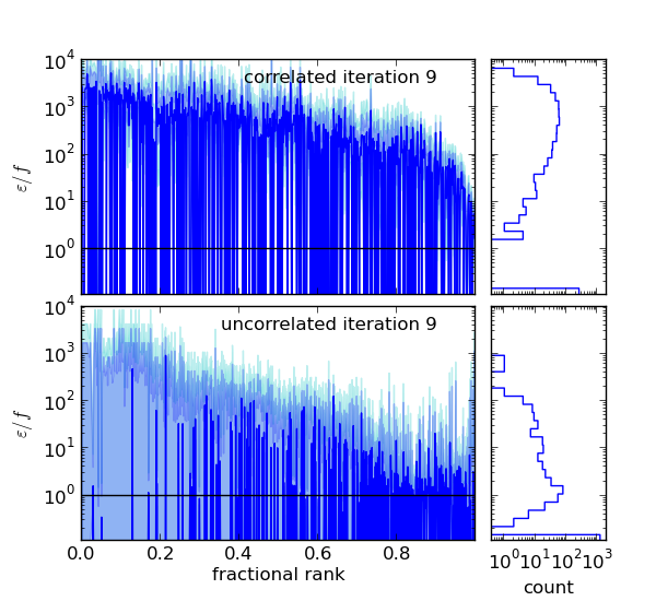
Figure 6: Comparison of OVL figure-of-merit upon evaluation using round-robin binning and correlated/uncorrelated data. We see that there are many configurations that perform poorly upon round-robin evaluation in both the correlated and uncorrelated data. However, we also see that the histograms of the two data sets are much different, with clearly separated points of maximum likelihood. Furthermore, the uncorrelated data appears to have a peak in likelihood near $\varepsilon/f\approx 1$, which is exactly what we expect from Poisson coincidence. The bin with $\varepsilon/f=0$ corresponds to configurations that do not find any conincident GW-channel events.

3.4 Effects of algorithmic parameters

OVL constructs a set of configurations based on a list of channels, thresholds, and time-windows, using all possible permutations of these parameters. In the bulk of this paper, we used time-windows from the set {25ms, 50ms, 100ms, 150ms, 200ms} and KW significance thresholds from the set {15, 25, 30, 50, 100, 200, 400, 800, 1600}. These thresholds and windows were chosen because they reflect the types of glitch significance and correlation time-scales observed in the past. We would expect that increasing the dimensionality of these configurations would allow the algorithm to better separate classes of glitches (characterized by the elements of the configuration).

Generally, we see that high auxiliary significance thresholds congregate at the top of the ordered list. This is because these events are relatively rare and are likely to be strongly correlated with GW-channel glitches. We contrast this with low threshold events, which are relatively common and may be more strongly influenced by a statistical background. This also means that these high-threshold auxiliary glitches are used first and dominate OVL’s performance at low dead-time. However, at sufficiently high dead-time, low-significance auxiliary glitches begin to dominate performance. Consider a set of veto configurations with the same auxiliary channel and significance threshold. Then, for a configuration from this set to remove more GW-channel glitches, it must widen the time-window applied around auxiliary glitches. If the GW-channel glitches are clustered, this can improve efficiency, but if the GW-channel glitches are sparse, it will mainly increase fractional dead-time without removing more glitches. However, lower threshold events may be able to better select small, widely separated GW-channel glitches without increasing the time-window used. Even if the correlation is weaker, this can increase overall performance. Similar effects are observed with the time-windows. Small time-windows typically show up at the top of the list with larger time windows appearing later and at decreased efficiency-over-deadtime.

4 Applications in instrument characterization

The OVL method we just described generates a wealth of information beyond the list of times that should be used as vetoes in a search for gravitational-wave transients. This information can be mined and used for general instrument monitoring and characterization. The algorithm is also simple and efficient enough so that to be able to analyze data within a few seconds from real time and without any significant impact on computational resources.

In giving a flavor of the capacity of our analysis, we will focus on the immediately derived quantities out of our statistical analysis. The typical output of our algorithm in the training phase is captured in Figure 2, where the most relevant auxiliary channels (and their corresponding parameters) are ranked using our unified criterion.

Table 2: This is an example OVL output from iteration 9 of the S6 data. We observe a nearly monotonic decrease in efficiency-over-deadtime as we proceed down the list. We also notice that several channels appear multiple times with different sets of significance thresholds and time-windows. In way of definition, livetime is the number of seconds in the analysis; #gwtrg is the number of GW-channel glitches in the analysis; vchan is the auxiliary channel name; vthr is the threshold on auxiliary KW significance; vwin is the time-window applied around each auxiliary glitch; deadsec is the number of seconds removed by this configuration; vexp is the expected number of GW-channel glitches coincident contained in deadsec; vact is the actual number of coincident GW-channel glitches; vsignif is the negative-logarithm of the Poisson significance of observing vact coincident GW-channel glitches when we expected vexp; eff is the efficiency; fdt is the fractional dead-time; eff/fdt is efficiency-over-deadtime, OVL’s ranking metric.

  livetime #gwtrg  vchn                               vthr   vwin deadsec  vexp vact vsignif  eff/fdt
374014.000   2826  L1_LSC-POB_Q_1024_4096              400  0.025   0.238  0.00    6   44.50  3334.29
374013.762   2820  L1_OMC-PZT_LSC_OUT_DAQ_8_1024      1600  0.025   1.500  0.01   32  225.00  2829.42
374012.262   2788  L1_OMC-PZT_LSC_OUT_DAQ_8_1024       400  0.025   0.550  0.00   11   77.97  2683.02
374011.712   2777  L1_ISI-OMC_GEOPF_H2_IN1_DAQ_8_1024 1600  0.100   0.150  0.00    3   22.19  2693.64
374011.562   2774  L0_PEM-LVEA_SEISZ_8_128             200  0.050   0.100  0.00    2   15.11  2696.55
374011.462   2772  L1_ISI-OMC_GEOPF_H1_IN1_DAQ_8_1024  400  0.025   0.266  0.00    5   35.94  2539.06
374011.196   2767  L1_OMC-PZT_LSC_OUT_DAQ_8_1024       200  0.025   0.541  0.00    9   62.50  2250.26
374010.656   2758  L1_OMC-PZT_LSC_OUT_DAQ_8_1024       100  0.025   0.908  0.01   14   95.28  2090.54
374009.747   2744  L1_ASC-ITMY_P_8_256                 400  0.025   3.700  0.03   56  374.35  2062.93
374006.047   2688  L0_PEM-LVEA_BAYMIC_8_1024           400  0.025   1.835  0.01   25  166.23  1895.94

The identification and ranking of channels that contribute to gravitational-wave-like glitches allows tracking such contributions over time, thus promptly signaling changes in the couplings between instrument channels and their environments. In Figure 7 we show an example of how auxiliary channels appear in OVL’s final training table (like the one in Figure 2) The colors reflect the significance of each channel in the corresponding veto configuration list, with dark red corresponding to high efficiency–over–dead-time and blue corresponding to low efficiency–over–dead-time. Applying simple thresholds either in the absolute significance or in the stride-by-stride changes in significance can provide useful handles in identifying and investigating changes in instrument performance.

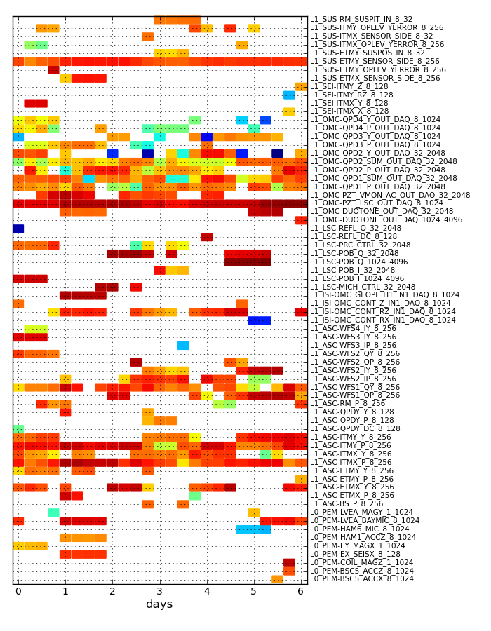
Figure 7: Appearance of auxiliary channels shown over the single week of S6 data. Channels’ relative performance is encoded in the color scheme, with dark red implying high $\varepsilon/f$ and blue low $\varepsilon/f$. Simple thresholding on absolute significance or relative changes in significance can provide handles for initiating and assisting investigations on instrument performance. We should note that the “L1” prefix on the channel names corresponds to the LIGO Livingston detector, and the last two numbers at the end of the channel name correspond to the bandwidth of that channel (in Hertz).

Zooming out to more macroscopic quantities, key summary quantities encoded in our ROC curves like efficiency and dead-time can be readily used for prompt figure-of-merit criteria when making data acquisition decisions as data come in. For example, by fixing a tolerable dead-time one can monitor the efficiency of the veto algorithm as a function of time, or in a symmetric way monitor the dead-time corresponding to a veto configuration that results in a fixed efficiency. We show one such example in Figure 8. In this plot the resulting efficiency in removing gravitational-wave-like glitches from the gravitational-wave channel over seven days of S6 data is shown at two arbitrary dead-times, one at 0.1% and another one at 0.01%.

The examples we have used above mostly target identification and studies of what has been a commonly encountered feature of the first generation gravitational-wave detectors, namely, non-stationarity. Our algorithm assists the study of such variability at the single-channel level as well as at the macroscopic level, in terms of quantities that will end up being relevant in an end-to-end search (like residual singles rates before and after veto application).

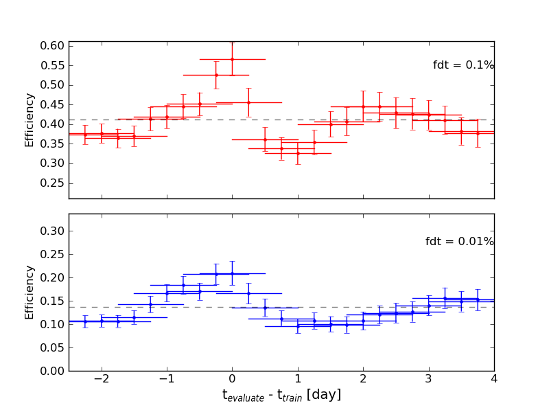
Figure 8: Efficiency at fixed fractional dead-time over 1 week of S6 data. This plot shows the change in performance for a single ordered list when it is applied on different days. The abscissa shows the time difference between the training and evaluation sets and we see that there is significane flucutation in performance, although those fluctuations appear to be bounded.

We should also note that OVL can be used to conduct safety studies, in which we determine which auxiliary channels are coupled to possible GW signals. The results presented in this paper are predicated on previous safety studies, conducted via hardware injections. However, OVL need not resort to these external studies. By running the OVL algorithm over a set of fake glitches corresponding to only hardware injections, OVL will naturally select the auxiliary channels that are highly correlated with these injections. By removing these auxiliary channels and re-processing the hardware injections, we can iteratively determine which auxiliary channels are unsafe and remove them from the analysis. Clearly, the procedure should terminate when OVL’s performance becomes consistent with uncorrelated data, and example of which is shown in Section 3.2. These safety studies can be repeated for various types of injections in order to determine which auxiliary channels are unsafe for certain classes of expected waveforms.

5 Conclusions

A variety of astrophysical sources of GWs are expected to produce short-duration signals within the sensitive frequency band of kilometer-scale ground-based interferometers, such as those operated by the LIGO, GEO600 and Virgo collaborations. Multiple terrestrial noise sources can produce transient artifacts (glitches) that resemble these short duration signals, and their contribution to the background for searches of these types of signals is a limiting factor for search sensitivity. An active area of research involves developing procedures to remove this transient noise during analysis of GW-channel data by using information derived from the many auxiliary channels which measure the local environment and other instrumental non-GW degrees of freedom. We presented the Ordered Veto List (OVL) algorithm, which aims to identify the unique and most relevant correlations between GW-channel glitches and similar signals seen in auxiliary channels by use of an iterative application and ranking of auxiliary channel veto conditions.

OVL uses many veto configurations to describe the types of couplings between auxiliary channels and the GW channel. This implementation used auxiliary channel name, a threshold on auxiliary glitch significance, and a time-window surrounding auxiliary glitches. However, the algorithm can be easily extended to include other parameters such as frequency information or time of day. OVL then constructs a list of segments using these configuration parameters. The union of time-windows surrounding auxiliary glitches with a sufficiently high significance is used to remove data from the GW channel. OVL then computes the configuration’s efficiency and dead-time, the fractions of GW-channel glitches and livetime removed, respectively. The configurations are then ranked according to the ratio of these numbers, efficiency-over-deadtime, which has the natural interpretation as the ratio of the number of removed GW-channel glitches and the expected number of removed GW-channel glitches. Furthermore, these configurations are applied hierarchically, in that once a configuration is applied, later configurations do not see any data removed by earlier configurations. Upon iteration, this repeated ranking and application finds highly correlated auxiliary channels and constructs an ordered list based on the efficiency-over-deadtimes observed. It also removes any redundant or uninformative channels.

This paper presented OVL results based on the entirety of LIGO S4 data (February 22, 2005 – March 25, 2005) from the LIGO Hanford Observatory (H1) and one week of LIGO S6 data (May 28, 2010 – June 4, 2010) from the LIGO Livingston Observatory (L1) using Kleine Welle glitches. These two data sets represent very different noise sources and couplings between auxiliary channels and the GW channel. Therefore, the common trends we observe in the two data sets are indicative of OVL itself, rather than any peculiarities within a data set.

We examined OVL’s performance using standard Receiver Operating Characteristic (ROC) curves, which shows the fraction of noise signals we are able to remove as a function of the fractional loss in live-time incurred. We see that the bulk performance is gained after 2 iterations, and this improves over the application of configurations based solely on their individual performance when applied to the entier data set. Further iteration helps to compress the useful information in the ordered list into a small number of configurations. This helps isolate exactly which correlations are significant and makes the list easier to read. We find that while the ROC curve only marginally improves between 2 and 9 iterations, the ordered list is only 1-2% as long after 9 iterations.

Finally, we point out a few possible applications of OVL to instrument characterization, including tracking and accounting for instrument non-stationarity and identification of subsystems containing channels that are highly correlated with GW-channel glitches.

References

References

- [1] Abbott B et al. (LIGO Scientific Collaboration) 2009 Rept.Prog.Phys. 72 076901 (Preprint 0711.3041)
- [2] Accadia T et al. (VIRGO Collaboration) 2012 JINST 7 P03012
- [3] Grote H (LIGO Scientific Collaboration) 2008 Class.Quant.Grav. 25 114043
- [4] Cutler C and Thorne K 2002 An overview of gravitational-wave sources General Relativity and Gravitation ed Bishop N and Maharaj S (Singapore; River Edge, U.S.A.: World Scientific) pp 72–111
- [5] Abadie J et al. (LIGO Scientific Collaboration, Virgo Collaboration) 2010 Phys.Rev. D82 102001 (Preprint 1005.4655)
- [6] Abadie J et al. (LIGO Collaboration, Virgo Collaboration) 2012 Phys.Rev. D85 082002 (Preprint 1111.7314)
- [7] Abadie J et al. (LIGO Collaboration, Virgo Collaboration) 2010 Phys.Rev. D81 102001 (Preprint 1002.1036)
- [8] Abadie J et al. (LIGO Scientific Collaboration, Virgo Collaboration) 2012 Phys.Rev. D85 122007 (Preprint 1202.2788)
- [9] Di Credico A (LIGO Scientific Collaboration) 2005 Class.Quant.Grav. 22 S1051–S1058 (Preprint gr-qc/0504106)
- [10] Christensen N, Shawhan P and Gonzalez G (LIGO Scientific Collaboration) 2004 Class.Quant.Grav. 21 S1747–S1756 (Preprint gr-qc/0403114)
- [11] Christensen N (LIGO Scientific Collaboration) 2005 Class.Quant.Grav. 22 S1059–S1068 (Preprint gr-qc/0504067)
- [12] Slutsky J, Blackburn L, Brown D, Cadonati L, Cain J et al. 2010 Class.Quant.Grav. 27 165023 (Preprint 1004.0998)
- [13] Isogai T (LIGO and Virgo Scientific Collaborations) 2010 J.Phys.Conf.Ser. 243 012005
- [14] Katsavounidis E and Shawhan P 2006 Veto selection for gravitational wave event searches lIGO-G060639-00-Z
- [15] Ajith P, Hewitson M, Smith J and Strain K 2006 Class.Quant.Grav. 23 5825–5837 (Preprint gr-qc/0605079)
- [16] Ajith P, Hewitson M, Smith J, Grote H, Hild S et al. 2007 Phys.Rev. D76 042004 (Preprint 0705.1111)
- [17] Biswas R et al. in preparation LIGO-P1300005
- [18] Blackburn L 2010 Open Issues in the Search for Gravitational Wave Transients Ph.D. thesis MIT
- [19] Abbott B et al. (LIGO Scientific Collaboration) 2009 Phys.Rev. D80 102001 (Preprint 0905.0020)
- [20] Smith J R, Abbott T, Hirose E, Leroy N, Macleod D et al. 2011 Class.Quant.Grav. 28 235005 (Preprint 1107.2948)
- [21] Chatterji S, Blackburn L, Martin G and Katsavounidis E 2004 Class.Quant.Grav. 21 S1809–S1818 (Preprint gr-qc/0412119)
- [22] Abbott B et al. (LIGO Scientific Collaboration) 2007 Class.Quant.Grav. 24 5343–5370 (Preprint 0704.0943)