Linear slices close to a Maskit slice

Abstract

We consider linear slices of the space of Kleinian once-punctured torus groups; a linear slice is obtained by fixing the value of the trace of one of the generators. The linear slice for trace $2$ is called the Maskit slice. We will show that if traces converge ‘horocyclically’ to $2$ then associated linear slices converge to the Maskit slice, whereas if the traces converge ‘tangentially’ to $2$ the linear slices converge to a proper subset of the Maskit slice. This result will be also rephrased in terms of complex Fenchel-Nielsen coordinates. In addition, we will show that there is a linear slice which is not locally connected.

1 Introduction

One of the central issues in the theory of Kleinian groups is to understand the structures of deformation spaces of Kleinian groups. In this paper we consider Kleinian punctured torus groups, one of the simplest classes of Kleinian groups with a non-trivial deformation theory.

Let $S$ be a once-punctured torus and let $R(S)$ be the space of conjugacy classes of representations $\rho:\pi_{1}(S)\to{\mathrm{PSL}}(2,\mathbb{C})$ which takes a loop surrounding the cusp to a parabolic element. The space $AH(S)$ of Kleinian punctured torus groups is the subset of $R(S)$ of faithful representations with discrete images. Although the interior of $AH(S)$ is parameterized by a product of Teichmüller spaces of $S$, its boundary is quite complicated. For example, McMullen [Mc2] showed that $AH(S)$ self-bumps, and Bromberg [Br] showed that $AH(S)$ is not even locally connected. We refer the reader to [Ca] for more information on the topology of deformation spaces of general Kleinian groups.

In this paper we investigate the shape of $AH(S)$ form the point of view of the trace coordinates. Let us fix a pair $a,b$ of generators of $\pi_{1}(S)$. Then every representation $\rho$ in $R(S)$ is essentially determined by the data $({\mathrm{tr}}\,\rho(a),{\mathrm{tr}}\,\rho(b))=(\alpha,\beta)\in\mathbb{C}^{2}$. Thus we identify $R(S)$ with $\mathbb{C}^{2}$ in this introduction (see Section 2 for more accurate treatment). We want to understand when $(\alpha,\beta)\in\mathbb{C}^{2}$ corresponds to a point of $AH(S)$. More precisely, we consider in this paper the shape the linear slice

$$\mathcal{L}(\beta):=\{\alpha\in\mathbb{C}:(\alpha,\beta)\in AH(S)\}$$

of $AH(S)$ when $\beta$ close to $2$. Note that $\mathcal{L}(2)$ is known as the Maskit slice, corresponding to the set of representations $\rho\in AH(S)$ such that $\rho(b)$ is parabolic. It is natural to ask the following question: “When $\beta$ tends to $2$, does $\mathcal{L}(\beta)$ converge to $\mathcal{L}(2)$?” Parker and Parkkonen [PP] studied this question in the case that a real number $\beta>2$ tends to $2$, and obtained an affirmative answer for this case. In this paper, we consider the question above in the general case that a complex number $\beta\in\mathbb{C}\setminus[-2,2]$ tends to $2$, and obtain the complete answer to this question. In fact, the answer depends on the manner how $\beta$ tends to $2$.

To describe our results, we need to introduce the notion of complex length. Let $\rho\in R(S)$ and assume that $\beta={\mathrm{tr}}\rho(b)$ is close to $2$. Then the complex length $\lambda$ of $\rho(b)$ is determined by the relation $\beta=2\cosh(\lambda/2)$ and the normalization $\mathrm{Re}\,\lambda>0,\,\mathrm{Im}\,\lambda\in(-\pi,\pi]$. We denote this $\lambda$ by $\lambda(\beta)$. Note that $\beta\to 2$ if and only if $\lambda(\beta)\to 0$. We say that a sequence $\beta_{n}\in\mathbb{C}\setminus[-2,2]$ converges horocyclically to $2$ if for any disk in the right-half plane $\mathbb{C}_{+}$ touching at zero, $\lambda(\beta_{n})$ are eventually contained in this disk. On the other hand, we say that the sequence $\beta_{n}$ converges tangentially to $2$ if there is a disk in $\mathbb{C}_{+}$ touching at zero which does not contain any $\lambda(\beta_{n})$. Now we can state our main result. (See Theorems 6.6 and 6.8 for more precise statements. See also Figure 3.)

Theorem 1.1.

Suppose that a sequence $\beta_{n}\in\mathbb{C}\setminus[-2,2]$ converges to $2$. If $\beta_{n}\to 2$ horocyclically, then $\mathcal{L}(\beta_{n})$ converge to $\mathcal{L}(2)$ in the sense of Hausdorff. On the other hand, if $\beta_{n}\to 2$ tangentially, then $\mathcal{L}(\beta_{n})$ converge (up to subsequence) to a proper subset of $\mathcal{L}(2)$ in the sense of Hausdorff.

We now sketch the essential idea which is underlying this phenomenon. Especially we explain the reason why the limit of linear slices is a proper subset of $\mathcal{L}(2)$ in the case where $\beta_{n}\to 2$ tangentially.

Now suppose that $\beta_{n}\to 2$ tangentially, and that a sequence $\alpha_{n}\in\mathcal{L}(\beta_{n})$ converges to $\alpha\in\mathbb{C}$. We will explain that $\alpha$ should lie in a proper subset of $\mathcal{L}(2)$. Let us take a sequence $\rho_{n}\in AH(S)$ such that $({\mathrm{tr}}\,\rho_{n}(a),{\mathrm{tr}}\,\rho_{n}(b))=(\alpha_{n},\beta_{n})$. Since $(\alpha_{n},\beta_{n})\to(\alpha,2)$ as $n\to\infty$, and since $AH(S)$ is closed, we have $(\alpha,2)\in AH(S)$, and hence $\alpha\in\mathcal{L}(2)$. By taking conjugations, we may assume that $\rho_{n}(a)\to A_{\alpha}$ and $\rho_{n}(b)\to B$ in ${\mathrm{PSL}}(2,\mathbb{C})$, where

$$A_{\alpha}=\left(\begin{array}[]{cc}\alpha&-i\\ -i&0\end{array}\right)\quad\text{and}\quad B=\left(\begin{array}[]{cc}1&2\\ 0&1\end{array}\right).$$

In addition, by pass to a subsequence if necessary, we may also assume that the sequence $\rho_{n}(\pi_{1}(S))$ converges geometrically to a Kleinian group $\Gamma$, which contains the algebraic limit $\langle A_{\alpha},B\rangle$. From the assumption that $\beta_{n}\to 2$ tangentially, one can see that the cyclic groups $\langle\rho_{n}(b)\rangle$ converge geometrically to rank-$2$ abelian group $\langle B,C\rangle$, where $C$ is of the form

$$C=\left(\begin{array}[]{cc}1&\zeta\\ 0&1\end{array}\right)$$

for some $\zeta\in\mathbb{C}\setminus\mathbb{R}$, see Theorem 6.5. Therefore the geometric limit $\Gamma$ contains the group $\langle A_{\alpha},B,C\rangle$. For any given integer $k$, one see from $C^{k}A_{\alpha}=A_{\alpha-ki\zeta}$ that the group $\langle A_{\alpha-ki\zeta},B\rangle$ is a subgroup of the Kleinian group $\Gamma$. Hence the group $\langle A_{\alpha-ki\zeta},B\rangle$ is discrete and thus $\alpha-ki\zeta\in\mathcal{L}(2)$. Therefore $\alpha$ should be contained in the intersection

$$\bigcap_{k\in\mathbb{Z}}(ki\zeta+\mathcal{L}(2)),$$

which is a proper subset of $\mathcal{L}(2)$.

In the proof of Theorem 1.1, we will make an essential use of Bromberg’s theory in [Br]. In fact, Bromberg obtained in [Br] a coordinate system for representations in $AH(S)$ close to the Maskit slice. The poof of Theorem 1.1 is then obtained by comparing Bromberg’s coordinates and the trace coordinates.

Some other topics and computer graphics of linear slices can be fond in [Mc2], [MSW] and [KY], as well as [PP].

This paper is organized as follows; In section 2, we recall some basic fact about spaces of representations and their subspaces. In section 3, we introduce the trace coordinates for the space $R(S)$ of representations of the once-punctured torus group. In section 4, we recall Bromberg’s theory in [Br] which gives us a local model of the space $AH(S)$ of Kleinian once-punctured torus groups near the Maskit slice. In section 5, we consider relation between Bromberg’s coordinates and the trace coordinates, and obtain an estimate which will be used in the proofs of the main results. We will show our main results, Theorems 6.6 and 6.8, in section 6. We also show that there is a linear slice which is not locally connected. In section 7, we translate our main results in terms of the complex Fenchel-Nielsen coordinates.

The following is the mainstream of this paper, where the top (resp. bottom) line is corresponding to the tangential (resp. horocyclic) convergence:

Acknowledgements.

The author would like to thank Hideki Miyachi for his many helpful discussions. He is also grateful to Keita Sakugawa for developing a computer program drawing linear slices, which was very helpful to proceed this research. All computer-generated figures of linear slices of this paper are made by this program.

2 Spaces of representations

In this section, we recall the definitions of spaces we will work with.

Let $(M,P)$ be a paired manifold; that is, $M$ is a compact, hyperbolizable $3$-manifold with boundary and $P$ is a disjoint union of tori and annuli in $\partial M$. Especially, every torus component of $\partial M$ is contained in $P$. Let

$${\cal R}(M,P):={\mathrm{Hom}}_{P}^{\mathrm{irr}}(\pi_{1}(M),{\mathrm{PSL}}(2,\mathbb{C}))$$

denote the set of all type-preserving, irreducible representations of $\pi_{1}(M)$ into ${\mathrm{PSL}}(2,\mathbb{C})$. Here a representation $\rho:\pi_{1}(M)\to{\mathrm{PSL}}(2,\mathbb{C})$ is said to be type-preserving if $\rho(\gamma)$ is parabolic or identity for every $\gamma\in\pi_{1}(P)$. The space of representations

$$R(M,P):={\cal R}(M,P)/{\mathrm{PSL}}(2,\mathbb{C})$$

is the set of all ${\mathrm{PSL}}(2,\mathbb{C})$-conjugacy classes $[\rho]$ of representations $\rho$ in ${\cal R}(M,P)$. We endow this space $R(M,P)$ with the algebraic topology; that is, a sequence $[\rho_{n}]$ converges to $[\rho]$ if there are representatives $\rho_{n}$ in $[\rho_{n}]$ and $\rho$ in $[\rho]$ such that for every $g\in\pi_{1}(M)$ the sequence $\rho_{n}(g)$ converges to $\rho(g)$ in ${\mathrm{PSL}}(2,\mathbb{C})$. The conjugacy class $[\rho]$ of a representation $\rho$ is also denoted by $\rho$ if there is no confusion. We are interested in the topological nature of the space

$$AH(M,P):=\{\rho\in R(M,P):\rho\text{ is faithful, discrete}\}.$$

It is known by Jørgensen [Jø] that $AH(M,P)$ is closed in $R(M,P)$. Let $MP(M,P)$ denote the subset of $AH(N,P)$ consists of representations $\rho$ which are minimally parabolic (i.e., $\rho(g)$ is parabolic if and only if $g\in\pi_{1}(P)$) and geometrically finite. It is known by Marden [Mar] and Sullivan [Su] that $MP(N,P)$ is equal to the interior of $AH(N,P)$ as a subset of $R(N,P)$. Recently, it was shown by Brock, Canary and Minsky [BCM] that the closure of $MP(M,P)$ is equal to $AH(M,P)$.

In this paper, we only consider the following three paired manifolds

$$(N,P),\quad(N,P^{\prime}),\quad({\hat{N}},{\hat{P}})$$

which are constructed as follows (see Figure 1):

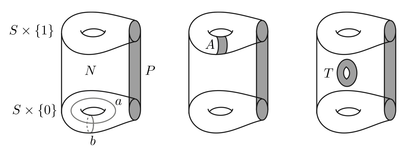
Figure 1: Paired manifolds $(N,P),(N,P^{\prime})$ and $({\hat{N}},{\hat{P}})$ (from left to right).

Let $S$ be a torus with one open disk removed. Throughout of this paper, we fix a pair $a,b$ of generators of $\pi_{1}(S)$ such that the geometric intersection number equals one. Then the commutator $[a,b]=aba^{-1}b^{-1}$ is homotopic to $\partial S$. Now we set

$$N:=S\times[0,1]$$

and

$$P:=\partial S\times[0,1].$$

We next set $P^{\prime}:=P\cup A$, where $A\subset S\times\{1\}$ is an annulus whose core curve is freely homotopic to $b\in\pi_{1}(S)$. Finally, we let

$$({\hat{N}},{\hat{P}}):=(N\setminus W,P\cup T),$$

where $W$ is a regular tubular neighborhood of $b\times\{1/2\}$ in $N=S\times[0,1]$ and $T:=\partial W$.

Note that $AH(N,P^{\prime})$ lies in the boundary of $AH(N,P)$; in fact $\rho\in AH(N,P)$ lies in $AH(N,P^{\prime})$ if and only if $\rho(b)$ is parabolic. This space $AH(N,P^{\prime})$ is called the Maskit slice of $AH(N,P)$. It is known by Minsky [Mi] that $AH(N,P^{\prime})$ has exactly two connected components. Bromberg’s theory in [Br] gives us an information about the topology of $AH(N,P)$ near $AH(N,P^{\prime})$. The aim of this paper is to understand the topology of $AH(N,P)$ near $AH(N,P^{\prime})$ from the view point of the trace coordinates, which is explained in the next section.

3 Trace coordinates for $AH(N,P)$

In this section, we introduce a trace coordinate system on a subset of $R(N,P)$ containing $R(N,P^{\prime})$.

Recall that $(N,P)=(S\times[0,1],\partial S\times[0,1])$, where $S$ is a torus with one open disk removed. In this case, the space $R(N,P)$ consists of all ${\mathrm{PSL}}(2,\mathbb{C})$-conjugacy classes of representations

$$\rho:\pi_{1}(S)=\langle a,b\rangle\to{\mathrm{PSL}}(2,\mathbb{C})$$

which satisfy the condition ${\mathrm{tr}}(\rho([a,b]))=-2$. Note that the trace of the commutator $[a,b]$ is well defined, although the traces of $\rho(a)$ and $\rho(b)$ are determined up to sign.

As we will see below, for any given $(\alpha,\beta)\in\mathbb{C}^{2}$, there is a representation $\rho\in R(N,P)$ which satisfies ${\mathrm{tr}}^{2}\rho(a)=\alpha^{2},\,{\mathrm{tr}}^{2}\rho(b)=\beta^{2}$, and this $\rho$ is determined uniquely up to pre-composition of automorphism $(a,b)\mapsto(a,b^{-1})$ of $\pi_{1}(N)$. Therefore the subset

$$\mathcal{D}_{{\mathrm{tr}}}:=\{(\alpha,\beta)\in\mathbb{C}^{2}:\exists\rho\in AH(N,P)\text{ s.t. }{\mathrm{tr}}^{2}\rho(a)=\alpha^{2},\,{\mathrm{tr}}^{2}\rho(b)=\beta^{2}\}$$

of $\mathbb{C}^{2}$ is well-defined. Note that the set $\mathcal{D}_{\mathrm{tr}}$ is symmetric under the action $(\alpha,\beta)\mapsto(\beta,\alpha)$. For a given $\beta\in\mathbb{C}$, the slice

$$\mathcal{L}(\beta):=\{\alpha\in\mathbb{C}:(\alpha,\beta)\in\mathcal{D}_{{\mathrm{tr}}}\}.$$

of $\mathcal{D}_{\mathrm{tr}}$ is called the linear slice for $\beta$. Note that $\mathcal{L}(\beta)$ is symmetric under the action of $z\mapsto-z$. The aim of this paper is to understand the shape of $\mathcal{L}(\beta)$ when $\beta$ is close to $2$.

To study the shape of linear slices, it would be convenient if we could identify $R(N,P)$ with $\mathbb{C}^{2}$ simply by $\rho\mapsto({\mathrm{tr}}\,\rho(a),{\mathrm{tr}}\,\rho(b))$. But the thing is not so simple. One reason is that traces of $\rho(a),\rho(b)$ are determined up to sign, and the other reason is that, for a given $(\alpha,\beta)\in\mathbb{C}^{2}$, there exist two candidate of representations $\rho$ which satisfy $({\mathrm{tr}}^{2}\rho(a),{\mathrm{tr}}^{2}\rho(b))=(\alpha^{2},\beta^{2})$. Therefore, in this section, we will choose an appropriate open domain $\Omega\subset R(N,P)$ so that there exists an embedding ${\mathrm{Tr}}:\Omega\to\mathbb{C}^{2}$ such that ${\mathrm{Tr}}(\rho)=(\alpha,\beta)$ satisfies $({\mathrm{tr}}^{2}\rho(a),{\mathrm{tr}}^{2}\rho(b))=(\alpha^{2},\beta^{2})$ for every $\rho\in\Omega$.

We begin by identifying $R(N,P^{\prime})$ with $\mathbb{C}$. For a given $\alpha\in\mathbb{C}$, let $\rho_{\alpha}$ be the representation in $R(N,P^{\prime})$ defined by

$$\rho_{\alpha}(a):=\left(\begin{array}[]{cc}\alpha&-i\\ -i&0\end{array}\right),\quad\rho_{\alpha}(b):=\left(\begin{array}[]{cc}1&2\\ 0&1\end{array}\right).$$

Then we have the following lemma. (See Lemma 4.3 in [Br]. Note that we are assuming that every element of $R(N,P^{\prime})$ is irreducible.)

Lemma 3.1.

The map $\psi:\mathbb{C}\to R(N,P^{\prime})$ defined by $\alpha\mapsto\rho_{\alpha}$ is a homeomorphism.

Note that the map $\psi$ in Lemma 3.1 induces a homeomorphism from $\mathcal{L}(2)$ onto the Maskit slice $AH(N,P^{\prime})$.

In the next lemma, we will show that the homeomorphism $\psi^{-1}:R(N,P^{\prime})\to\mathbb{C}$ naturally extends to an embedding from an open domain $\Omega\subset R(N,P)$ containing $R(N,P^{\prime})$ into $\mathbb{C}^{2}$.

Lemma 3.2.

There exist an open, connected, simply connected domain $\Omega\subset R(N,P)$ and a homeomorphism

$${\mathrm{Tr}}:\Omega\to\mathbb{C}^{2}$$

which satisfy the following:

1. $\Omega$ contains $R(N,P^{\prime})$, and ${\mathrm{Tr}}$ takes $R(N,P^{\prime})$ onto $\mathbb{C}\times\{2\}$. In addition, we have ${\mathrm{Tr}}(\rho_{\alpha})=(\alpha,2)$ for every $\alpha\in\mathbb{C}$.

2. For every $\rho\in\Omega$, ${\mathrm{Tr}}(\rho)=(\alpha,\beta)$ satisfies ${\mathrm{tr}}^{2}\rho(a)=\alpha^{2}$ and ${\mathrm{tr}}^{2}\rho(b)=\beta^{2}$.

Throughout of this paper, we fix such a domain $\Omega$. We call ${\mathrm{Tr}}$ the trace coordinate map and $(\alpha,\beta)={\mathrm{Tr}}(\rho)$ the trace coordinates of $\rho\in\Omega$. The rest of this section is devoted to the proof of this lemma. The commutative diagram (3.2) should be helpful for understanding the arguments. The reader may skip this proof by admitting Lemma 3.2.

To show Lemma 3.2, it is convenient to consider the space $\widetilde{R}(N,P)$ of representations of $\pi_{1}(N)$ into ${\mathrm{SL}}(2,\mathbb{C})$, instead of ${\mathrm{PSL}}(2,\mathbb{C})$. More precisely, the set $\widetilde{R}(N,P)$ consists of ${\mathrm{SL}}(2,\mathbb{C})$-conjugacy classes of representations $\tilde{\rho}$ of $\pi_{1}(S)$ into ${\mathrm{SL}}(2,\mathbb{C})$ which satisfy the condition ${\mathrm{tr}}(\tilde{\rho}([a,b]))=-2$. The ${\mathrm{SL}}(2,\mathbb{C})$-conjugacy class of $\tilde{\rho}$ is also denoted by $\tilde{\rho}$ if there is no confusion. It is well known that an element $\tilde{\rho}$ of $\widetilde{R}(N,P)$ is uniquely determined by the triple $({\mathrm{tr}}\tilde{\rho}(a),{\mathrm{tr}}\tilde{\rho}(b),{\mathrm{tr}}\tilde{\rho}(ab))$ of complex number (see for example [Bo] or [Go]):

Lemma 3.3.

The map

$$\widetilde{\mathrm{Tr}}:\widetilde{R}(N,P)\to\Xi:=\{(\alpha,\beta,\gamma)\in\mathbb{C}^{3}:\alpha^{2}+\beta^{2}+\gamma^{2}=\alpha\beta\gamma\}\setminus\{(0,0,0)\}$$

defined by $\tilde{\rho}\mapsto({\mathrm{tr}}\tilde{\rho}(a),{\mathrm{tr}}\tilde{\rho}(b),{\mathrm{tr}}\tilde{\rho}(ab))$ is a homeomorphism.

By using this lemma, we often identify $\widetilde{R}(N,P)$ with the subset $\Xi$ of $\mathbb{C}^{3}$. For $(\alpha,\beta)\in\mathbb{C}^{2}$, the numbers $\gamma$ satisfying $\alpha^{2}+\beta^{2}+\gamma^{2}=\alpha\beta\gamma$ are given by

$$\gamma=\frac{1}{2}\left(\alpha\beta\pm\sqrt{\alpha^{2}\beta^{2}-4(\alpha^{2}+\beta^{2})}\right).$$

Therefore the projection

$$\Pi:\Xi\to\mathbb{C}^{2}\setminus\{(0,0)\}$$

defined by $(\alpha,\beta,\gamma)\mapsto(\alpha,\beta)$ is a two-to-one branched covering map. If we denote by $\gamma_{1},\gamma_{2}$ the solutions of the equation $\alpha^{2}+\beta^{2}+\gamma^{2}=\alpha\beta\gamma$ on $\gamma$, we have $\gamma_{1}+\gamma_{2}=\alpha\beta$. On the other hand, we have

$${\mathrm{tr}}(AB)+{\mathrm{tr}}(AB^{-1})={\mathrm{tr}}A\,{\mathrm{tr}}B$$

for every $A,B\in{\mathrm{SL}}(2,\mathbb{C})$. Therefore one see that if two representations $\tilde{\rho}_{1},\tilde{\rho}_{2}$ in $\widetilde{R}(N,P)$ have the same image under the map $\Pi\circ\widetilde{\mathrm{Tr}}$, they are only differing by pre-composition of the automorphism $(a,b)\mapsto(a,b^{-1})$ of $\pi_{1}(S)$.

Now let

$$\pi:\widetilde{R}(N,P)\to R(N,P)$$

be the natural projection, which is a four-to-one covering map. The group of covering transformation for $\pi$ is isomorphic to $\mathbb{Z}_{2}\times\mathbb{Z}_{2}$ which is generated by $(\alpha,\beta,\gamma)\mapsto(-\alpha,\beta,-\gamma)$ and $(\alpha,\beta,\gamma)\mapsto(\alpha,-\beta,-\gamma)$, where $\widetilde{R}(N,P)$ is identified with $\Xi\subset\mathbb{C}^{3}$ as in Lemma 3.3.

Now let us take an open, connected and simply connected domain $\Delta\subset\mathbb{C}^{2}\setminus\{(0,0)\}$ which satisfy the following:

1. $\Delta$ contains the set $\mathbb{C}\times\{2\}$, and

2. $\Delta$ lies in the set $\{(\alpha,\beta)\in\mathbb{C}^{2}:\mathrm{Re}\,\beta>0,\,\alpha^{2}\beta^{2}\neq 4(\alpha^{2}+\beta^{2})\}$.

Here, the condition $\alpha^{2}\beta^{2}\neq 4(\alpha^{2}+\beta^{2})$ is equivalent to the condition that the pair $(\alpha,\beta)$ is not a critical value of the projection $\Pi:\Xi\to\mathbb{C}^{2}\setminus\{(0,0)\}$. Throughout of this paper, we fix such a domain $\Delta$.

Since $\alpha^{2}\beta^{2}\neq 4(\alpha^{2}+\beta^{2})$ for every $(\alpha,\beta)\in\Delta$, and since $\Delta$ is connected and simply connected, one can take a univalent branch of the square root of $\alpha^{2}\beta^{2}-4(\alpha^{2}+\beta^{2})$ on $\Delta$. We take the branch such that the value for $(\alpha,2)\in\Delta$ is equal to $-4i$. Then we obtain the univalent branch of

$$\gamma=\gamma(\alpha,\beta)=\frac{1}{2}\left(\alpha\beta+\sqrt{\alpha^{2}\beta^{2}-4(\alpha^{2}+\beta^{2})}\right)$$ (3.1)

on $\Delta$, and hence the univalent branch $\theta:\Delta\to\Xi$ of $\Pi^{-1}$ on $\Delta$.

Lemma 3.4.

The map $\pi\circ\widetilde{\mathrm{Tr}}^{-1}\circ\theta:\Delta\to R(N,P)$ is a homeomorphism onto its image.

Proof.

We only need to show that the orbit of $\theta(\Delta)$ under the action of $\mathbb{Z}_{2}\times\mathbb{Z}_{2}$ on $\Xi$ are mutually disjoint. Take two points $(\alpha,\beta),(\alpha^{\prime},\beta^{\prime})\in\Delta$. Suppose for contradiction that $(\alpha,\beta,\gamma(\alpha,\beta)),(\alpha^{\prime},\beta^{\prime},\gamma(\alpha^{\prime},\beta^{\prime}))\in\Xi$ are equivalent under the action of non-trivial element of the covering transformation group $\mathbb{Z}_{2}\times\mathbb{Z}_{2}$. Since $\mathrm{Re}\,\beta>0$ and $\mathrm{Re}\,\beta^{\prime}>0$, one see that $(\alpha^{\prime},\beta^{\prime},\gamma(\alpha^{\prime},\beta^{\prime}))=(-\alpha,\beta,-\gamma(\alpha,\beta))$. Then from (3.1) we have

$$\gamma(\alpha^{\prime},\beta^{\prime}) = \frac{1}{2}\left(\alpha^{\prime}\beta^{\prime}+\sqrt{\alpha^{\prime 2}\beta^{\prime 2}-4(\alpha^{\prime 2}+\beta^{\prime 2})}\right)$$

$$= \frac{1}{2}\left(-\alpha\beta+\sqrt{\alpha^{2}\beta^{2}-4(\alpha^{2}+\beta^{2})}\right).$$

But this with $\gamma(\alpha^{\prime},\beta^{\prime})=-\gamma(\alpha,\beta)$ implies $\sqrt{\alpha^{2}\beta^{2}-4(\alpha^{2}+\beta^{2})}=0$, which contradicts to $(\alpha,\beta)\in\Delta$. ∎

Now let

$$\Omega:=\pi\circ\widetilde{\mathrm{Tr}}^{-1}\circ\theta(\Delta)$$

and

$${\mathrm{Tr}}:=\left(\pi\circ\widetilde{\mathrm{Tr}}^{-1}\circ\theta\right)^{-1}:\Omega\to\Delta.$$

Then we obtain the following commutative diagram:

(3.6)

To show that this $\Omega$ and ${\mathrm{Tr}}$ satisfy the desired property in Lemma 3.2, we only need to show that ${\mathrm{Tr}}(\rho_{\alpha})=(\alpha,2)$ for every $\alpha\in\mathbb{C}$. This can be seen from the following two facts: (i) If we regard $\rho_{\alpha}=\psi(\alpha)$ as an element of $\widetilde{R}(N,P)$, we have $\widetilde{\mathrm{Tr}}(\rho_{\alpha})=(\alpha,2,\alpha-2i)$. (ii) From our choice of the branch $\theta$, we have $\theta(\alpha,2)=(\alpha,2,\alpha-2i)$. Thus we complete the proof of Lemma 3.2.

4 Bromberg’s coordinates for $AH(N,P)$

This section is devoted to explain the theory of Bromberg in [Br], which tells us the topology of $AH(N,P)$ near the Maskit slice $AH(N,P^{\prime})$. In fact, Bromberg construct a subset of $\mathbb{C}\times\hat{\mathbb{C}}$ such that $AH(N,P)$ is locally homeomorphic to this set at every point in $MP(N,P^{\prime})$.

4.1 The Maskit slice

Given $\mu\in\mathbb{C}$, we define a representation $\sigma_{\mu}\in R(N,P^{\prime})$ by

$$\sigma_{\mu}(a):=\left(\begin{array}[]{cc}-i\mu&-i\\ -i&0\end{array}\right),\quad\sigma_{\mu}(b):=\left(\begin{array}[]{cc}1&2\\ 0&1\end{array}\right).$$

This representation $\sigma_{\mu}$ is nothing but the representation $\rho_{\alpha}$ with $\alpha=-i\mu$, which is defined in the previous section. The subset

$$\mathcal{M}:=\{\mu\in\mathbb{C}:\sigma_{\mu}\in AH(N,P^{\prime})\}$$

of $\mathbb{C}$ is also called the Maskit slice. Since that the map $\mathbb{C}\to R(N,P^{\prime})$ defined by $\mu\mapsto\sigma_{\mu}$ is a homeomorphism from Lemma 3.1, $\mathcal{M}$ is homeomorphic to $AH(N,P^{\prime})$, and the interior $\mathrm{int}(\mathcal{M})$ of $\mathcal{M}$ is homeomorphic to $MP(N,P^{\prime})$. Since $\mu\in\mathcal{M}$ if and only if $-i\mu\in\mathcal{L}(2)$, we have

$$\mathcal{L}(2)=i\mathcal{M}=\{i\mu:\mu\in\mathcal{M}\}.$$

Note that $\mathcal{M}$ is invariant under the translation $\mu\mapsto\mu+2$. We refer the reader to [KS] for basic properties of $\mathcal{M}$. It is known by Minsky (Theorem B in [Mi]) that $\mathcal{M}$ has two connected components $\mathcal{M}^{+},\,\mathcal{M}^{-}$, where $\mathcal{M}^{+}$ contained in the upper half-plane and $\mathcal{M}^{-}$ is the complex conjugation of $\mathcal{M}^{+}$

4.2 Coordinates for $AH({\hat{N}},{\hat{P}})$

We now introduce a coordinate system on the space $AH({\hat{N}},{\hat{P}})$. Recall that $\hat{N}$ is $N$ minus a regular tubular neighborhood $W$ of $b\times\{1/2\}$, and $\hat{P}$ is a union of $P$ and $T=\partial W$. Bromberg’s idea in [Br] is that the space $AH({\hat{N}},{\hat{P}})$ can be used as a local model of $AH(N,P)$ near a point of $AH(N,P^{\prime})$.

The fundamental group of ${\hat{N}}$ is expressed as

$$\pi_{1}(\hat{N})=\langle a,b,c:[b,c]=\mathit{id}\rangle,$$

where $a,b$ is the pair of generators of the fundamental group of $S\times\{0\}\subset{\hat{N}}$, and $c$ is freely homotopic to an essential simple closed curve on $T$ that bounds a disk in $W$. We regard $\pi_{1}(T)=\langle b,c\rangle$. The space $R(\hat{N},\hat{P})$ of representations for $({\hat{N}},{\hat{P}})$ is expressed as

$$R(\hat{N},\hat{P})=\{\rho:\pi_{1}(\hat{N})\to{\mathrm{PSL}}(2,\mathbb{C}):{\mathrm{tr}}\rho([a,b])=-2,\,{\mathrm{tr}}^{2}\rho(c)=4\}/{\mathrm{PSL}}(2,\mathbb{C}).$$

For a given $(\mu,\zeta)\in\mathbb{C}^{2}$, we define a representation $\hat{\sigma}_{\mu,\zeta}\in R({\hat{N}},{\hat{P}})$ by

$$\hat{\sigma}_{\mu,\zeta}(a):=\sigma_{\mu}(a),\quad\hat{\sigma}_{\mu,\zeta}(b):=\sigma_{\mu}(b),\quad\hat{\sigma}_{\mu,\zeta}(c):=\left(\begin{array}[]{cc}1&\zeta\\ 0&1\end{array}\right).$$

Then we have the following:

Lemma 4.1 (Lemma 4.5 in [Br]).

The map $\mathbb{C}^{2}\to R({\hat{N}},{\hat{P}})$ defined by $(\mu,\zeta)\mapsto\hat{\sigma}_{\mu,\zeta}$ is a homeomorphism.

Remark.

Following the rule of notation in [Br], the representation $\hat{\sigma}_{\mu,\zeta}$ should be written as $\sigma_{\mu,\zeta}$. But we reserve the notation $\sigma_{\mu,\zeta}$ for another representation, which will be defined in the next subsection.

We define a subset $\mathcal{B}$ of $\mathbb{C}^{2}$ by

$$\mathcal{B}:=\{(\mu,\zeta)\in\mathbb{C}^{2}:\hat{\sigma}_{\mu,\zeta}\in AH({\hat{N}},{\hat{P}})\}.$$

Then, by the above lemma, the map

$$\mathcal{B}\to AH({\hat{N}},{\hat{P}})$$

defined by $(\mu,\zeta)\mapsto\hat{\sigma}_{\mu,\zeta}$ is a homeomorphism. Note that $(\mu,\zeta)\in\mathcal{B}$ implies $\mu\in\mathcal{M}$ since the restriction of $\hat{\sigma}_{\mu,\zeta}$ to the subgroup ${\langle a,b\rangle}$ of $\pi_{1}({\hat{N}})$ is equal to $\sigma_{\mu}$. Note also that if $\mathrm{Im}\,\zeta=0$ then $(\mu,\zeta)\not\in\mathcal{B}$; in fact, if $\mathrm{Im}\,\zeta=0$, it violates discreteness or faithfulness of the representation $\hat{\sigma}_{\mu,\zeta}$.

For any $(\mu,\zeta)\in\mathcal{B}$, the quotient manifold $\hat{M}={\bf H}^{3}/\hat{\sigma}_{\mu,\zeta}(\pi_{1}({\hat{N}}))$ is homeomorphic to the interior of ${\hat{N}}$, and has a rank-2 cusp whose monodromy group is the rank-2 parabolic subgroup of ${\mathrm{PSL}}(2,\mathbb{C})$ generated by $\hat{\sigma}_{\mu,\zeta}(b)$ and $\hat{\sigma}_{\mu,\zeta}(c)$. Since

$$\hat{\sigma}_{\mu,\zeta}(c^{-k}a)=\left(\begin{array}[]{cc}-i(\mu-k\zeta)&-i\\ -i&0\end{array}\right)\quad\text{and}\quad\hat{\sigma}_{\mu,\zeta}(b)=\left(\begin{array}[]{cc}1&2\\ 0&1\end{array}\right),$$

one can see that if $(\mu,\zeta)\in\mathcal{B}$ then $\mu-k\zeta\in\mathcal{M}$ for every $k\in\mathbb{Z}$. Bromberg showed that the converse is also true if $\mathrm{Im}\,\zeta\neq 0$ (see Proposition 4.7 in [Br]):

Theorem 4.2 (Bromberg).

Let $(\mu,\zeta)\in\mathbb{C}^{2}$ with $\mathrm{Im}\,\zeta\neq 0$. Then $(\mu,\zeta)\in\mathcal{B}$ if and only if $\mu-k\zeta\in\mathcal{M}$ for every integer $k$.

4.3 Bromberg’s coordinates for $AH(N,P)$

Following [Br], we now introduce a coordinate system on $AH(N,P)$ by using the coordinate system on $AH({\hat{N}},{\hat{P}})$ introduced in the previous subsection.

Now let

$$\mathcal{B}^{+}:=\{(\mu,\zeta)\in\mathcal{B}:\mathrm{Im}\,\zeta>0\}$$

and define a set $\mathcal{A}\subset\mathbb{C}\times\hat{\mathbb{C}}$ by

$$\mathcal{A}:=\mathcal{B}^{+}\cup(\mathcal{M}\times\{\infty\}).$$

The following theorem due to Bromberg claim that the set $\mathcal{A}$ can be used for a local model of $AH(N,P)$ at every point of $MP(N,P^{\prime})\subset AH(N,P)$.

Theorem 4.3 (Bromberg (Theorem 4.13 in [Br])).

For any $\nu\in\mathrm{int}(\mathcal{M})$, there exist a neighborhood $U$ of $(\nu,\infty)$ in $\mathcal{A}$, a neighborhood $V$ of $\sigma_{\nu}$ in $AH(N,P)$, and a homeomorphism $\Phi:U\to V.$

Remark.

Although Bromberg restricted to the case that $\nu\in\mathrm{int}(\mathcal{M}^{+})$ in [Br], it is obvious that the same argument works well for $\nu\in\mathrm{int}(\mathcal{M}^{-})$.

In this situation, we say that $(\mu,\zeta)\in U$ is Bromberg’s coordinates of the representation $\Phi(\mu,\zeta)\in V$. In what follows, we also write

$$\sigma_{\mu,\zeta}:=\Phi(\mu,\zeta).$$

We now briefly explain the definition of the map $\Phi:U\to V,\ (\mu,\zeta)\mapsto\sigma_{\mu,\zeta}$ to what extent we need in the following argument. See [Br] for the full details. Given $\nu\in\mathrm{int}(\mathcal{M})$, a neighborhood $U$ of $(\nu,\infty)$ in $\mathcal{A}$ is chosen sufficiently small so that the following argument works well. Let $(\mu,\zeta)\in U$. If $\zeta=\infty$ then $\sigma_{\mu,\infty}$ is defined to be $\sigma_{\mu}$. If $\zeta\neq\infty$, the quotient manifold

$$\hat{M}_{\mu,\zeta}={\bf H}^{3}/\hat{\sigma}_{\mu,\zeta}(\pi_{1}({\hat{N}}))$$

has a rank-$2$ cusp whose monodromy group is generated by $\hat{\sigma}_{\mu,\zeta}(b)$ and $\hat{\sigma}_{\mu,\zeta}(c)$. Since we are choosing $U$ sufficiently small, it follows from the filling theorem due to Hodgson, Kerckhoff and Bromberg (see Theorem 2.5 in [Br]) that there exists a $c$-filling $M_{\mu,\zeta}$ of $\hat{M}_{\mu,\zeta}$ for every $(\mu,\zeta)\in U$ with $\zeta\neq\infty$. More precisely, there is a complete hyperbolic manifold $M_{\mu,\zeta}$ homeomorphic to the interior of $N$ and an embedding

$$\phi_{\mu,\zeta}:\hat{M}_{\mu,\zeta}\to M_{\mu,\zeta}$$

which satisfy the following properties:

1. the image of $\phi_{\mu,\zeta}$ is equals to $M_{\mu,\zeta}$ minus the geodesic representative of $(\phi_{\mu,\zeta})_{*}(\hat{\sigma}_{\mu,\zeta}(b))$,

2. $(\phi_{\mu,\zeta})_{*}(\hat{\sigma}_{\mu,\zeta}(c))$ is trivial in $\pi_{1}(M_{\mu,\zeta})$, and

3. $\phi_{\mu,\zeta}$ extends to a conformal map between the conformal boundaries of $\hat{M}_{\mu,\zeta}$ and $M_{\mu,\zeta}$.

The map $\phi_{\mu,\zeta}$ is called the $c$-filling map. We will define $\sigma_{\mu,\zeta}$ to be an element in $AH(N,P)$ associated to $M_{\mu,\zeta}$. To this end, we need to determine a marking $N\to M_{\mu,\zeta}$. Since the restriction of the representation $\hat{\sigma}_{\mu,\zeta}$ to the subgroup $\langle a,b\rangle\subset\pi_{1}({\hat{N}})$ is equal to $\sigma_{\mu}$, the manifold $M_{\mu}={\bf H}^{3}/\sigma_{\mu}(\pi_{1}(N))$ covers $\hat{M}_{\mu,\zeta}$. The covering map is denoted by

$$\Pi_{\mu,\zeta}:M_{\mu}\to\hat{M}_{\mu,\zeta}.$$

Let $f_{\mu}:N\to M_{\mu}$ be a homotopy equivalence which induces $\sigma_{\mu}$. Then $\sigma_{\mu,\zeta}$ is defined to be a representation of $\pi_{1}(N)$ into ${\mathrm{PSL}}(2,\mathbb{C})$ induced form $\phi_{\mu,\zeta}\circ\Pi_{\mu,\zeta}\circ f_{\mu}$;

$$\begin{CD}N@>{f_{\mu}}>{\text{marking}}>M_{\mu}@>{\Pi_{\mu,\zeta}}>{\text{covering}}>\hat{M}_{\mu,\zeta}@>{\phi_{\mu,\zeta}}>{\text{filling}}>M_{\mu,\zeta}.\end{CD}$$

This $\sigma_{\mu,\zeta}$ is faithful, and hence, is contained in $AH(N,P)$ (see Lemma 3.6 in [Br]). Note from the construction of $\sigma_{\mu,\zeta}$ that the geodesic in $M_{\mu,\zeta}$ associated to $\sigma_{\mu,\zeta}(a)$ is homotopic to the image of the geodesic $\hat{M}_{\mu,\zeta}$ associated to $\hat{\sigma}_{\mu,\zeta}(a)$ by $\phi_{\mu,\zeta}$.

5 Relation between the trace coordinates and Bromberg’s coordinates

Let us consider the situation in Theorem 4.3. We may assume that $V$ is contained in the domain $\Omega$ of the trace coordinate map. In this section, we will study the relation between Bromberg’s coordinates $(\mu,\zeta)\in U$ of $\sigma_{\mu,\zeta}\in V$ and its trace coordinates $(\alpha,\beta)={\mathrm{Tr}}(\sigma_{\mu,\zeta})$. More precisely, we will observe in Theorem 5.1 that $(\mu,\zeta)$ is approximated by $(i\alpha,4\pi i/\lambda(\beta))$, where $\lambda(\beta)=2\cosh^{-1}(\beta/2)$ is the complex length of $\sigma_{\mu,\zeta}(b)$.

5.1 Complex length

For any element $g\in{\mathrm{PSL}}(2,\mathbb{C})$, its complex length $l(g)\in\mathbb{C}$ is a value which satisfies

$${{\mathrm{tr}}^{2}g}=4\cosh^{2}\left(\frac{l(g)}{2}\right).$$

If $g$ is not parabolic, this is equivalent to say that $g$ is conjugate to the Möbius transformation $z\mapsto e^{l(g)}z$. For a loxodromic element $g\in{\mathrm{PSL}}(2,\mathbb{C})$, its complex length $l(g)$ determined uniquely if we take it in the set

$$\Lambda:=\{z\in\mathbb{C}:\mathrm{Re}\,z>0,\,-\pi<\mathrm{Im}\,z\leq\pi\}.$$

In what follows, we always assume that $\l(g)\in\Lambda$ for loxodromic transformation $g$.

We now want to fix one-to-one correspondence between the complex length $l(g)$ of loxodromic element $g\in{\mathrm{SL}}(2,\mathbb{C})$ and its trace ${\mathrm{tr}}\,g$. Note that the map $z\mapsto 2\cosh(z/2)$ takes the interior of $\Lambda$ into the right-half plane

$$\mathbb{C}_{+}:=\{z\in\mathbb{C}:\mathrm{Re}\,z>0\}.$$

We define a map

$$\lambda:\mathbb{C}_{+}\setminus(0,2)\to\Lambda$$

as its inverse. Then we have

$$\lambda(z) = 2\cosh^{-1}\left(\frac{z}{2}\right)$$

$$= 2(z-2)^{1/2}+o(z-2)\quad(z\to 2),$$

where the real part of a square root is chosen positive. We have

$$\lambda({\mathrm{tr}}\,g)=l(g)$$

for every loxodromic element $g\in{\mathrm{SL}}(2,\mathbb{C})$ with ${\mathrm{tr}}\,g\in\mathbb{C}_{+}\setminus(0,2]$.

5.2 Main estimates

The following theorem tells us a relation between Bromberg’s coordinates and the trace coordinates for representations close to the Maskit slice.

Theorem 5.1.

Let $\nu\in\mathrm{int}(\mathcal{M})$. For any $\epsilon>0$, we can choose a neighborhoods $U$ of $(\nu,\infty)$ and $V$ of $\sigma_{\nu}$ in Theorem 4.3 so that they also satisfy the following: $V$ is contained in the domain $\Omega$ of the trace coordinate map, and for any $(\mu,\zeta)\in U$ with $\zeta\neq\infty$, we have

1. $|\mu-i\alpha|\leq\epsilon$, and

2. $|\zeta-4\pi i/\lambda(\beta)|\leq\epsilon\,\mathrm{Im}\,\zeta$,

where $(\alpha,\beta)={\mathrm{Tr}}(\sigma_{\mu,\zeta})$ is the trace coordinates of $\sigma_{\mu,\zeta}$

Remark.

These estimates 1 and 2 follow from the fact that we can choose the $c$-filling map $\phi_{\mu,\zeta}:\hat{M}_{\mu,\zeta}\to M_{\mu,\zeta}$ close to the isometry outside a neighborhood of the rank-$2$ cusp. Then the estimates 1 and 2 are obtained from estimates due to McMullen (Lemma 3.20 in [Mc1]) and Magid (Theorem 1.2 in [Mag]), respectively.

Proof of Theorem 5.1.

Let us take a neighborhood $U$ of $(\nu,\infty)$ in $\mathcal{A}$, a neighborhood $V$ of $\sigma_{\nu}$ in $AH(N,P)$ and a homeomorphism $\Phi:U\to V$ as in the statement of Theorem 4.3. We may assume that $V\subset\Omega$. We will show below that estimates 1 and 2 are obtained if we modify $U$ sufficiently small.

For $(\mu,\zeta)\in U$ with $\zeta\neq\infty$, let

$$\phi_{\mu,\zeta}:\hat{M}_{\mu,\zeta}\to M_{\mu,\zeta}$$

be the $c$-filling map. To control the distortion of the map $\phi_{\mu,\zeta}$, we need to recall the notion of normalized length.

Suppose that $\delta>0$ is less than the Margulis constant for hyperbolic 3-manifolds, and let $\mathbb{T}_{\delta}(T)$ denote the component of $\delta$-thin part of $\hat{M}_{\mu,\zeta}$ associated to the rank-2 cusp. We endow the boundary $\partial\mathbb{T}_{\delta}(T)$ of $\mathbb{T}_{\delta}(T)$ with the natural Euclidean metric. The marking map $\hat{N}\to\hat{M}_{\mu,\zeta}$ induces a marking map $T\to\partial\mathbb{T}_{\delta}(T)$. Via this marking, the pair of generators $b,c$ of $\pi_{1}(T)$ are also regarded as the pair of generators of $\pi_{1}(\partial\mathbb{T}_{\delta}(T))$. In this setting, the normalized length $L(c)$ of the free homotopy class of $c\subset\partial\mathbb{T}_{\delta}(T)$ is defined by

$$L(c):=\frac{\mathrm{length}(c^{\prime})}{\sqrt{\mathrm{Area}(\partial\mathbb{T}_{\delta}(T))}},$$

where $\mathrm{length}(c^{\prime})$ is the Euclidean length of the geodesic representative $c^{\prime}$ of $c$ in $\partial\mathbb{T}_{\delta}(T)$. This $L(c)$ does not depend on the choice of $\delta$. Since

$$\hat{\sigma}_{\mu,\zeta}(b)=\left(\begin{array}[]{cc}1&2\\ 0&1\end{array}\right)\quad\text{and}\quad\hat{\sigma}_{\mu,\zeta}(c)=\left(\begin{array}[]{cc}1&\zeta\\ 0&1\end{array}\right),$$

the normalized length $L(c)$ can be calculated concretely as

$$L(c)=\frac{|\zeta|}{\sqrt{2\,\mathrm{Im}\,\zeta}}.$$

For any given $K>0$, we can choose the neighborhood $U$ sufficiently small so that for all $(\mu,\zeta)\in U$ with $\zeta\neq\infty$, the normalized length $L(c)$ of $c$ at the rank-$2$ cusp of $\hat{M}_{\mu,\zeta}$ is greater than $K$. We will show below that if we take such $K$ sufficiently large, the estimates 1 and 2 hold.

We may assume that there is a uniform upper bound of $|\mu|$ for $(\mu,\zeta)\in U$. Then, since ${\mathrm{tr}}^{2}\hat{\sigma}_{\mu,\zeta}(a)=-\mu^{2}$, there is an upper bound $R>0$ for hyperbolic lengths of geodesic representatives $a^{*}$ of $\hat{\sigma}_{\mu,\zeta}(a)$ in $\hat{M}_{\mu,\zeta}$ for all $(\mu,\zeta)\in U$ with $\zeta\neq\infty$. Therefore we can take $\delta>0$ small enough so that the unit neighborhood ${\cal N}(a^{*},1)$ of $a^{*}$ in $\hat{M}_{\mu,\zeta}$ does not intersect the $\delta$-thin part $\mathbb{T}_{\delta}(T)\subset\hat{M}_{\mu,\zeta}$ for all $(\mu,\zeta)\in U$ with $\zeta\neq\infty$.

It follows from the filling theorem due to Hodgson, Kerckhoff and Bromberg (see Theorem 2.5 in [Br]) that for $\delta>0$ chosen as above and for any $\epsilon_{1}>0$, there exists $K>0$ such that if the normalized length of $c$ in $\hat{M}_{\mu,\zeta}$ is greater than $K$ then the $c$-filling map can be chosen so that it restricts to a $(1+\epsilon_{1})$-bi-Lipschitz diffeomorphism

$$\phi_{\mu,\zeta}:\hat{M}_{\mu,\zeta}\setminus\mathbb{T}_{\delta}(T)\to M_{\mu,\zeta}\setminus\mathbb{T}_{\delta}(b^{*}),$$

where $\mathbb{T}_{\delta}(b^{*})\subset M_{\mu,\zeta}$ is the $\delta$-Margulis tube of the geodesic representative $b^{*}$ of $\sigma_{\mu,\zeta}(b)$; i.e., the core curve of the filled torus in $M_{\mu,\zeta}$. We can now apply a theorem of McMullen (Lemma 3.20 in [Mc1]) to obtain

$$|{\mathrm{tr}}^{2}(\hat{\sigma}_{\mu,\zeta}(a))-{\mathrm{tr}}^{2}(\sigma_{\mu,\zeta}(a))|<C(R)\epsilon_{1},$$

where $C(R)>0$ is a constant which depends only on $R$. (Recall that $R$ is the upper bounds of the hyperbolic length of $a^{*}$.) Since ${\mathrm{tr}}^{2}\,\hat{\sigma}_{\mu,\zeta}(a)=-\mu^{2}$, ${\mathrm{tr}}^{2}\,\sigma_{\mu,\zeta}(a)=\alpha^{2}$, and since $\alpha$ is close to $-i\mu$, we obtain

$$|\mu-i\alpha|<\epsilon$$

for a given $\epsilon>0$ by taking $K$ large enough. Thus we obtain the first estimate.

We next show the second estimate. One can expect to obtain this kind of estimate since the Teichmüller parameter of the torus $\partial\mathbb{T}_{\delta}(T)\subset\hat{M}_{\mu,\zeta}$ with respect to the generators $b,c$ is equal to $\zeta/2$ and that of $\partial\mathbb{T}_{\delta}(b^{*})\subset M_{\mu,\zeta}$ is equal to $2\pi i/\lambda(\beta)$, and since there is a bi-Lipschitz map of small distortion between these tori. Magid accomplish this estimate in [Mag]. In fact, by simplifying his estimates (ii) and (iv) of Theorem 1.2 in [Mag], we see that there is some constant $C>0$ such that if the normalized length $L(c)=|\zeta|/\sqrt{2\,\mathrm{Im}\,\zeta}$ of $c$ is sufficiently large, we have

$$\left|\lambda(\beta)-\frac{4\pi i}{\zeta}\right|\leq C\frac{(\mathrm{Im}\,\zeta)^{2}}{|\zeta|^{4}}=\frac{4C}{L(c)^{4}}.$$ (5.1)

One can also see from $L(c)=|\zeta|/\sqrt{2\,\mathrm{Im}\,\zeta}$ that $\mathrm{Re}(4\pi i/\zeta)=2\pi/L(c)^{2}$. Combining this with (5.1), we have

$$|\lambda(\beta)|>\frac{1}{2}\left|\frac{4\pi i}{\zeta}\right|=\frac{2\pi}{|\zeta|}$$ (5.2)

for $L(c)$ large enough. Finally, multiplying $|\zeta/\lambda(\beta)|$ on both sides of (5.1) and using the estimate (5.2), we obtain

$$\left|\zeta-\frac{4\pi i}{\lambda(\beta)}\right|\leq C^{\prime}\frac{(\mathrm{Im}\zeta)^{2}}{|\zeta|^{2}}=\frac{C^{\prime}}{2L(c)^{2}}\mathrm{Im}\,\zeta<\epsilon\,\mathrm{Im}\,\zeta$$

for a given $\epsilon>0$ if $L(c)$ is large enough. Thus we obtain the second estimate. ∎

5.3 $\mathcal{A}$ and $\mathcal{D}$

Since the shape of $\mathcal{A}$ is well understood from Theorem 4.2, we can expect to understand the shape of $\mathcal{D}_{\mathrm{tr}}$ from that of $\mathcal{A}$. To apply Theorem 5.1, it is convenient to consider the image of the set $\mathcal{D}_{\mathrm{tr}}$ by the transformation $(\alpha,\beta)\mapsto(i\alpha,4\pi i/\lambda(\beta))$. More precisely, we define a map

$$F:\mathbb{C}\times(\mathbb{C}_{+}\setminus(0,2))\to\mathbb{C}\times\hat{\mathbb{C}}$$

by

$$F(z,w):=\left(iz,\frac{4\pi i}{\lambda(w)}\right)$$

and set

$$\mathcal{D}_{\mathrm{tr}}^{+}:=\{(\alpha,\beta)\in\mathcal{D}_{\mathrm{tr}}:\beta\in\mathbb{C}_{+}\}$$

and

$$\mathcal{D}:=F(\mathcal{D}_{\mathrm{tr}}^{+}).$$

Note that, since we are interested in the shape of $\mathcal{D}_{\mathrm{tr}}$ where the second entry is close to $2$, we may restrict our attention to $\mathcal{D}_{\mathrm{tr}}^{+}$. Note also that $F(z,2)=(iz,\infty)$ for every $z$.

Let us now consider the situation of Theorem 5.1. We define a homeomorphism $\varphi$ from $U$ onto its domain by $\varphi=F\circ{\mathrm{Tr}}\circ\Phi$;

$$\begin{CD}\varphi:U@>{\Phi}>{}>V@>{{\mathrm{Tr}}}>{}>\mathcal{D}_{\mathrm{tr}}@>{F}>{}>\mathcal{D}.\end{CD}$$

Then by definition we have $\varphi(\mu,\infty)=(\mu,\infty)$ for any $(\mu,\infty)\in U$. It follows from Theorem 5.1 the point $\varphi(\mu,\zeta)$ is close to $(\mu,\zeta)\in U$ even if $\zeta\neq\infty$. Therefore, we expect that the shape of $\mathcal{A}$ is similar to that of $\mathcal{D}$ in a neighborhood of $(\nu,\infty)$ for every $\nu\in\mathrm{int}(\mathcal{M})$.

We will justify this expectation in Propositions 5.2 and 5.3 below. In what follows, we denote by $B_{\epsilon}(z)$ the $\epsilon$-neighborhood of $z$ in $\mathbb{C}$, and by $B_{\epsilon}(z,w)$ the $\epsilon$-neighborhood of $(z,w)$ in $\mathbb{C}^{2}$.

Proposition 5.2.

For any $\nu\in\mathrm{int}(\mathcal{M})$, there exists $\epsilon_{0}>0$ which satisfy the following: For any $0<\epsilon<\epsilon_{0}$ and $I>0$, there exists $K>0$ such that for all $z\in\mathbb{C}$ with $|z|>K$ and $0<\mathrm{Im}\,z<I$, $B_{\epsilon}(\nu,z)\subset\mathcal{A}$ implies $B_{\epsilon/2}(\nu,z)\subset\mathcal{D}.$

Proof.

For any fixed $\nu\in\mathrm{int}(\mathcal{M})$, let us take neighborhoods $U\subset\mathcal{A}$, $W\subset\mathcal{D}$ of $(\nu,\infty)$ such that $\varphi=F\circ{\mathrm{Tr}}\circ\Phi$ is a homeomorphism from $U$ onto $W$. We may assume that $U$ is of the form

$$U=\mathcal{A}\cap\{(\mu,\zeta)\in\mathbb{C}^{2}:|\mu-\nu|<\epsilon_{0},|\zeta|>K/2\}$$

for some $\epsilon_{0}>0$ and $K>0$. Let us take $0<\epsilon<\epsilon_{0}$ and $I>0$ arbitrarily. One can see from Theorem 5.1 and its proof that if we choose $K$ large enough, we may also assume that

$$d_{\mathbb{C}^{2}}(\varphi(\mu,\zeta),(\mu,\zeta))<\frac{\epsilon}{8}$$ (5.3)

holds for every $(\mu,\zeta)\in U$ with $0<\mathrm{Im}\,\zeta<2I$. (Note that if $|\zeta|\to\infty$ then $|\zeta|/\sqrt{2\mathrm{Im}\,\zeta}\to\infty$.)

Now let us take $z\in\mathbb{C}$ with $|z|>K$ and $0<\mathrm{Im}\,z<I$, and suppose that $B_{\epsilon}(\nu,z)\subset\mathcal{A}$. Then $B_{\epsilon}(\nu,z)\subset U$ and $0<\mathrm{Im}\,\zeta<2I$ for every $(\mu,\zeta)\in B_{\epsilon}(\nu,z)$ (since $K$ and $I$ are larger than $\epsilon$). Thus the inequality (5.3) holds for every $(\mu,\zeta)\in B_{\epsilon}(\nu,z)$. Using this fact, we will show that

$$B_{\epsilon/2}(\nu,z)\subset\varphi(B_{\epsilon}(\nu,z)),$$

which implies that $B_{\epsilon/2}(\nu,z)\subset\mathcal{D}$.

Suppose for contradiction that there exists some $p\in B_{\epsilon/2}(\nu,z)\setminus\varphi(B_{\epsilon}(\nu,z))$. Let consider a line segment

$$\gamma(t):=(1-t)\varphi(p)+tp,\quad t\in[0,1]$$

in $\mathbb{C}^{2}$ which joins $\varphi(p)$ to $p$. Since $d_{\mathbb{C}^{2}}(\varphi(p),p)<\epsilon/8$ and $p\in B_{\epsilon/2}(\nu,z)$, we have $\gamma([0,1])\subset B_{5\epsilon/8}(\nu,z)$. Now let

$$t_{\infty}:=\inf\{t:\gamma(t)\not\in\varphi(B_{\epsilon}(\nu,z))\}.$$

Since $\varphi(p)$ lies in $\varphi(B_{\epsilon}(\nu,z))$ but $p$ does not, and since $\varphi(B_{\epsilon}(\nu,z))$ is open, one see that $0<t_{\infty}\leq 1$. Let take an increasing sequence $t_{n}\to t_{\infty}\,(n\to\infty)$ and let $q_{n}:=\varphi^{-1}(\gamma(t_{n}))\in B_{\epsilon}(\nu,z)$. Since $\varphi(q_{n})(=\gamma(t_{n}))$ lie in $B_{5\epsilon/8}(\nu,z)$ and $d_{\mathbb{C}^{2}}(\varphi(q_{n}),q_{n})<\epsilon/8$, we have $q_{n}\in B_{3\epsilon/4}(\nu,z)$ for all $n$. Therefore an accumulation point $q_{\infty}$ of $\{q_{n}\}$ lies in $B_{\epsilon}(\nu,z)$. It follows form the continuity of $\varphi$ that $\varphi(q_{\infty})=\gamma(t_{\infty})$. Since $\varphi$ is local homeomorphism at $q_{\infty}$, this contradicts the definition of $t_{\infty}$. Thus we obtain $B_{\epsilon/2}(\nu,z)\subset\varphi(B_{\epsilon}(\nu,z))\subset\mathcal{D}$. ∎

We set

$$B_{\epsilon,I}(\nu):=B_{\epsilon}(\nu)\times\{z\in\mathbb{C}:\mathrm{Im}\,z>I\}.$$

Proposition 5.3.

For any $\nu\in\mathrm{int}(\mathcal{M})$, there exists $\epsilon_{0}>0$ which satisfy the following: For any $0<\epsilon<\epsilon_{0}$ there is $I>0$ such that $B_{\epsilon,I}(\nu)\subset\mathcal{A}$ implies $B_{\epsilon/2,2I}(\nu)\subset\mathcal{D}.$

Proof.

The proof is almost parallel to that of Proposition 5.2. For any fixed $\nu\in\mathrm{int}(\mathcal{M})$, let us consider the homeomorphism $\varphi:U\to W$ as in the proof of Proposition 5.2. One can see from Theorem 4.2 that there exist $\epsilon_{0}>0$ and $I>0$ such that $B_{\epsilon_{0},I}(\nu)\subset U$. Now let us take $0<\epsilon<\epsilon_{0}$ arbitrarily. Theorem 5.1 implies that if we choose $I$ large enough, we have the following: for any $(\mu,\zeta)\in B_{\epsilon,I}(\nu)$, $(\mu^{\prime},\zeta^{\prime}):=\varphi(\mu,\zeta)$ satisfies $|\mu^{\prime}-\mu|<\epsilon/8$ and $|\zeta^{\prime}-\zeta|<(\epsilon/8)\,\mathrm{Im}\,\zeta$. Using this fact, we can show that

$$B_{\epsilon/2,2I}(\nu)\subset\varphi(B_{\epsilon,I}(\nu)),$$

which implies that $B_{\epsilon/2,2I}(\nu)\subset\mathcal{D}$. The remaining argument is almost the same to that of Proposition 5.2, so we leave it for the reader. ∎

6 Main Results

In this section, we will show our main results, Theorems 6.6 and 6.8. More precisely, for a given sequence $\beta_{n}\in\mathbb{C}\setminus[-2,2]$ converging to $2$, we consider the Hausdorff limit of the linear slices $\mathcal{L}(\beta_{n})$ and the Carathéodory limit of the interiors $\mathrm{int}(\mathcal{L}(\beta_{n}))$ of the linear slices.

6.1 Horizontal slices of $\mathcal{A}$

We first consider horizontal slices of $\mathcal{A}$, which will appear as limits of linear slices. Let $\mathcal{M}(\zeta)$ denote the slice of $\mathcal{A}$ by fixing the second entry $\zeta\in\mathbb{C}\cup\{\infty\}$ in the product structure; that is,

$$\mathcal{M}(\zeta):=\{\mu\in\mathbb{C}:(\mu,\zeta)\in\mathcal{A}\}.$$

By definition of $\mathcal{A}$, one see that (i) $\mathcal{M}(\zeta)$ lies in $\mathcal{M}$ for every $\zeta$, (ii) $\mathcal{M}(\zeta)$ is empty if $\mathrm{Im}\,\zeta\leq 0$, and that (iii) $\mathcal{M}(\infty)=\mathcal{M}$. It follows from Theorem 4.2 that if $\mathrm{Im}\,\zeta>0$ the set $\mathcal{M}(\zeta)$ can be written as

$$\mathcal{M}(\zeta)=\bigcap_{k\in\mathbb{Z}}(k\zeta+\mathcal{M}),$$ (6.1)

where $k\zeta+\mathcal{M}=\{k\zeta+\mu:\mu\in\mathcal{M}\}$. (Note that (6.1) does not hold if $\mathrm{Im}\,\zeta\leq 0$.) Note that $\mathcal{M}(\zeta)$ is invariant under the action of $\langle z+2,z+\zeta\rangle$. It is known by Wright [Wr] that the stripe $\{z\in\mathbb{C}:-1\leq\mathrm{Im}\,z\leq 1\}$ does not intersect $\mathcal{M}$. Therefore one see that $\mathcal{M}(\zeta)=\emptyset$ if $0<\mathrm{Im}\,\zeta\leq 2$.

We now consider relationship between horizontal slices of $\mathcal{A}$ and linear slices, or horizontal slices of $\mathcal{D}_{\mathrm{tr}}$. By definition, we have

$$\alpha\in\mathcal{L}(\beta)\ \iff\ (\alpha,\beta)\in\mathcal{D}_{\mathrm{tr}}\ \iff\ \left(i\alpha,\frac{4\pi i}{\lambda(\beta)}\right)\in\mathcal{D}$$

and

$$\left(i\alpha,\frac{4\pi i}{\lambda(\beta)}\right)\in\mathcal{A}\ \iff\ \alpha\in i\mathcal{M}\left(\frac{4\pi i}{\lambda(\beta)}\right).$$

Recall from Theorem 5.1 that $(\mu,\zeta)\in\mathcal{A}$ is almost equivalent to $(\mu,\zeta)\in\mathcal{D}$ if $\mu$ lies in $\mathrm{int}(\mathcal{M})$ and $|\zeta|$ is large enough. Therefore we may expect that $\mathcal{L}(\beta)$ is similar to $i\mathcal{M}({4\pi i/\lambda(\beta)})$ when $\beta$ is close to $2$. We will justify this observation below. To this end, we first recall the definitions of Hausdorff convergence and Carathéodory convergence.

Definition 6.1 (Hausdorff convergence).

Let $F_{n}\ (n\in\mathbb{N}),\,F_{\infty}$ be closed subsets in $\mathbb{C}$. We say that the sequence $F_{n}$ converges $F_{\infty}$ in the sense of Hausdorff if the following two conditions are satisfied:

1. For any $x_{\infty}\in F_{\infty}$, there is a sequence $x_{n}\in F_{n}$ such that $x_{n}\to x_{\infty}$.

2. If there is a sequence $x_{n_{j}}\in F_{n_{j}}$ such that $x_{n_{j}}\to x_{\infty}$, then $x_{\infty}\in F_{\infty}$.

Definition 6.2 (Carathéodory convergence).

Let $\Omega_{n}\ (n\in\mathbb{N}),\,\Omega_{\infty}$ be open subsets in $\mathbb{C}$. We say that the sequence $\Omega_{n}$ converges to $\Omega_{\infty}$ in the sense of Carathéodory if the following two conditions are satisfied:

1. For any compact subset $X$ of $\Omega_{\infty}$, $X\subset\Omega_{n}$ for all large $n$.

2. If there is an open subset $O$ of $\mathbb{C}$ and an infinite sequence $\{n_{j}\}_{j=1}^{\infty}$ such that $O\subset\Omega_{n_{j}}$, then $O\subset\Omega_{\infty}$.

Note that closed subsets $F_{n}\subset\mathbb{C}$ converge to $F_{\infty}\subset\mathbb{C}$ in the sense of Hausdorff if and only of their complements $\mathbb{C}\setminus F_{n}$ converge to $\mathbb{C}\setminus F_{\infty}$ in the sense of Carathéodory.

The next lemma implies that $\mathcal{M}(\zeta_{n})$ converge to $\mathcal{M}$ if and only if $\mathrm{Im}\,\zeta_{n}\to\infty$, which is a direct consequence of (6.1):

Lemma 6.3.

Suppose that a sequence $\{\zeta_{n}\}_{n=1}^{\infty}$ in $\mathbb{C}$ with $\mathrm{Im}\,\zeta_{n}>0$ converges to $\infty$ in $\hat{\mathbb{C}}$. Then the followings are equivalent:

1. $\mathrm{Im}\,\zeta_{n}\to\infty$ as $n\to\infty$.

2. $\mathcal{M}({\zeta_{n}})$converge to $\mathcal{M}$ in the sense of Hausdorff as $n\to\infty$.

3. $\mathrm{int}(\mathcal{M}({\zeta_{n}}))$ converge to $\mathrm{int}(\mathcal{M})$ in the sense of Carathéodory as $n\to\infty$.

6.2 Horocyclic and tangential convergence

To describe our main theorems, we also need the following definition (see Figure 1):

Definition 6.4.

Suppose that a sequence $\{\lambda_{n}\}_{n=1}^{\infty}$ in the right-half plane $\mathbb{C}_{+}=\{z\in\mathbb{C}\,|\,\mathrm{Re}\,z>0\}$ converges to $0$. We say that $\lambda_{n}\to 0$ horocyclically if for any $\epsilon>0$, $|\lambda_{n}-\epsilon|<\epsilon$ for all large $n$, and that $\lambda_{n}\to 0$ tangentially if there is a constant $\epsilon_{0}>0$ such that $|\lambda_{n}-\epsilon_{0}|>\epsilon_{0}$ for all $n$.

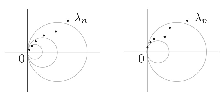
Figure 2: Horocyclic convergence (left) and tangential convergence (right).

Note that $\lambda_{n}\to 0$ horocyclically if and only if $|\mathrm{Im}(2\pi i/\lambda_{n})|\to\infty$, and that tangentially if and only if $|\mathrm{Im}(2\pi i/\lambda_{n})|$ are uniformly bounded above.

When a sequence $\beta_{n}\in\mathbb{C}\setminus[-2,2]$ converges to $2$, the limit of the sequence $\mathcal{L}(\beta_{n})$ depends on whether $\lambda(\beta_{n})\to 0$ horocyclically or tangentially. The essence of the difference between horocyclic and tangential convergence can be found in the next theorem on geometric limits of cyclic groups, which was first observed by Jørgensen. See, for example, Theorem 3.3 in [It] for the proof.

We say that a sequence of discrete subgroups $G_{n}$ of ${\mathrm{PSL}}(2,\mathbb{C})$ converges geometrically to a subgroup $G$ of ${\mathrm{PSL}}(2,\mathbb{C})$ if $G_{n}$ converge to $G$ in the sense of Hausdorff as closed subsets of ${\mathrm{PSL}}(2,\mathbb{C})$.

Theorem 6.5.

Suppose that a sequence $B_{n}$ of loxodromic elements converges to

$$B=\left(\begin{array}[]{cc}1&2\\ 0&1\end{array}\right)$$

in ${\mathrm{PSL}}(2,\mathbb{C})$. Let $\lambda_{n}$ denote the complex length of $B_{n}$. Then we have the following:

1. If $\lambda_{n}\to 0$ horocyclically, then the sequence $\langle B_{n}\rangle$ converges geometrically to $\langle B\rangle$.

2. Suppose that $\lambda_{n}\to 0$ tangentially. We further assume that there exists a complex number $\xi$ with $\mathrm{Im}\,\xi\geq 0$ and a sequence $m_{n}$ of integers with $|m_{n}|\to\infty$ such that

   $$\lim_{n\to\infty}\left(\frac{2\pi i}{\lambda_{n}}-m_{n}\right)=\xi.$$

   In this situation, we have

   $$\lim_{n\to\infty}B_{n}^{-m_{n}}=C:=\left(\begin{array}[]{cc}1&2\xi\\ 0&1\end{array}\right).$$

   In addition, if $\mathrm{Im}\,\xi\neq 0$, the sequence $\langle B_{n}\rangle$ converges geometrically to the rank-$2$ parabolic group $\langle B,C\rangle$.

Remark.

When $\lambda_{n}\to 0$ tangential, there is a constant $M>0$ such that $0<\mathrm{Im}(2\pi i/\lambda_{n})<M$ for every $n$. Therefore we may assume that, by pass to a subsequence if necessary, the sequence $2\pi i/\lambda(\beta_{n})$ converges to some $\xi\in\mathbb{C}$ with $\mathrm{Im}\,\xi\geq 0$ up to the action of $z\mapsto z+1$.

6.3 Main theorem for tangential convergence

We can now state our main theorem for linear slices $\mathcal{L}(\beta_{n})$ such that $\lambda(\beta_{n})$ converge tangentially to $0$. See Figure 3, left column.

Theorem 6.6.

Let $\{\beta_{n}\}_{n=1}^{\infty}$ be a sequence in $\mathbb{C}\setminus[-2,2]$ which converges to $2$ as $n\to\infty$. Suppose that $\lambda(\beta_{n})$ converge tangentially to $0$. We further assume that there exists a complex number $\xi$ with $\mathrm{Im}\,\xi\geq 0$ and a sequence $m_{n}$ of integers with $|m_{n}|\to\infty$ such that

$$\lim_{n\to\infty}\left(\frac{2\pi i}{\lambda(\beta_{n})}-m_{n}\right)=\xi.$$

Then we have the following:

1. $\mathcal{L}(\beta_{n})$ converge to $i\mathcal{M}({2\xi})$ in the sense of Hausdorff as $n\to\infty$.

2. $\mathrm{int}(\mathcal{L}(\beta_{n}))$ converge to $\mathrm{int}(i\mathcal{M}({2\xi}))$ in the sense of Carathéodory as $n\to\infty$.

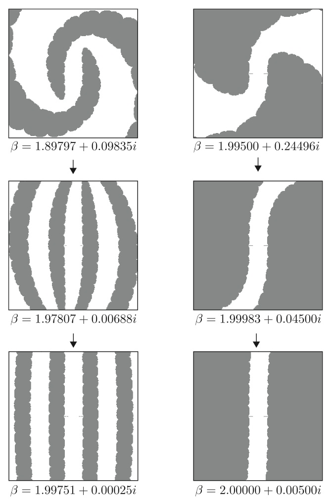
Figure 3: Computer-generated figure of linear slices $\mathcal{L}(\beta)$ (gray parts) for $\beta$ close to $2$, restricted to the square of width $24$ centered at $0$. Left column corresponds to tangential convergence $\lambda(\beta)\to 0$, where $\lambda(\beta)$ are points on the circle $|z-1|=1$ whose imaginary part equal $0.7$ (top), $0.3$ (middle) and $0.1$ (bottom). Right column corresponds to horocyclic convergence $\lambda(\beta)\to 0$, where $\lambda(\beta)$ equal $0.7+0.7i$ (top), $0.3+0.3i$ (middle) and $0.1+0.1i$ (bottom).

The following lemma is an essential part of the proof of Theorem 6.6.

Lemma 6.7.

Under the same assumption as in Theorem 6.6, we have the following: For any $\alpha\in\mathrm{int}(i\mathcal{M}({2\xi}))$ there exists $\epsilon>0$ such that $B_{\epsilon}(\alpha)\subset\mathrm{int}(\mathcal{L}(\beta_{n}))$ for all large $n$.

Proof.

Suppose that $\alpha\in\mathrm{int}(i\mathcal{M}({2\xi}))$. Then $(i\alpha,2\xi)\in\mathrm{int}(\mathcal{A})$. Let $\epsilon_{0}>0$ be the constant in Proposition 5.2 for $\nu=i\alpha$. Since $(i\alpha,2\xi)\in\mathrm{int}(\mathcal{A})$, one can find $0<\epsilon<\epsilon_{0}$ such that $B_{\epsilon}(i\alpha,2\xi)\subset\mathcal{A}$. Since the set $\mathcal{A}$ is invariant under the action $(z,w)\mapsto(z,w+2)$, we have $B_{\epsilon}(i\alpha,2\xi+2m_{n})\subset\mathcal{A}$. Let $K>0$ be the constant in Proposition 5.2 for $\epsilon>0$ chosen above and $I=\mathrm{Im}(2\xi)+1$. Since $|m_{n}|\to\infty$ as $n\to\infty$, we have $|2\xi+2m_{n}|>K$ for all large $n$. Then by Proposition 5.2, we have

$$B_{\epsilon/2}(i\alpha,2\xi+2m_{n})\subset\mathcal{D}$$

for all large $n$. On the other hand, since the sequence $\{2\pi i/\lambda(\beta_{n})-m_{n}\}$ converges to $\xi$ as $n\to\infty$, we have

$$\left|\frac{4\pi i}{\lambda(\beta_{n})}-(2\xi+2m_{n})\right|<\epsilon/4$$

for all large $n$. Therefore

$$B_{\epsilon/4}\left(i\alpha,\frac{4\pi i}{\lambda(\beta_{n})}\right)\subset\mathcal{D}$$

hold for all large $n$. Thus we obtain $B_{\epsilon/4}(\alpha)\subset\mathrm{int}(\mathcal{L}(\beta_{n}))$ for all large $n$. ∎

Proof of Theorem 6.6.

We need to prove the following four conditions (H1), (H2), (C1) and (C2), where (H1) and (H2) are corresponding to the Hausdorff convergence and (C1) and (C2) are corresponding to the Carathéodory convergence:

(H1)

For any $\alpha\in i\mathcal{M}({2\xi})$ there exists a sequence $\alpha_{n}\in\mathcal{L}(\beta_{n})$ such that $\alpha_{n}\to\alpha$.

(H2)

If $\alpha_{n_{j}}\in\mathcal{L}(\beta_{n_{j}})$ and $\alpha_{n_{j}}\to\alpha$ then $\alpha\in i\mathcal{M}({2\xi})$.

(C1)

For any compact subset $X\subset\mathrm{int}(i\mathcal{M}({2\xi}))$, $X\subset\mathrm{int}(\mathcal{L}(\beta_{n}))$ for all large $n$.

(C2)

If there exist an open subset $O\subset\mathbb{C}$ and a infinite sequence $\{n_{j}\}_{j=1}^{\infty}$ such that $O\subset\mathrm{int}(\mathcal{L}(\beta_{n_{j}}))$, then $O\subset\mathrm{int}(i\mathcal{M}({2\xi}))$.

Proof of (H1): For any $\alpha\in i\mathcal{M}({2\xi})$, there exists a sequence $\{\alpha(j)\}_{j=1}^{\infty}$ in the interior of $i\mathcal{M}({2\xi})$ such that $\alpha(j)\to\alpha$ as $j\to\infty$. It follows from Lemma 6.7 that for every $j$, there exists positive constant $N(j)$ such that $\alpha(j)\in\mathcal{L}(\beta_{n})$ for all $n\geq N(j)$. Thus we obtain the result. To be more precise, let us choose $\{N(j)\}_{j=1}^{\infty}$ so that $N(j+1)>N(j)$ and $N(j)\to\infty$ as $j\to\infty$, and set $\alpha_{n}:=\alpha(j)$ for every $N(j)\leq n<N(j)$. Since $j\to\infty$ as $n\to\infty$, we obtain $\alpha_{n}\in\mathcal{L}(\beta_{n})$ and $\alpha_{n}\to\alpha$ as $n\to\infty$.

Proof of (C1): Let $X$ be a compact subset of $\mathrm{int}(i\mathcal{M}({2\xi}))$. For every $\alpha\in X$, it follows from Lemma 6.7 that there exist $\epsilon(\alpha)>0$ and $N(\alpha)>0$ such that $B_{\epsilon(\alpha)}(\alpha)\subset\mathrm{int}(\mathcal{L}(\beta_{n}))$ for all $n\geq N(\alpha)$. Since

$$\bigcup_{\alpha\in X}B_{\epsilon(\alpha)}(\alpha)$$

is an open covering of the compact set $X$, we can choose finite set of points $\{\alpha_{j}\}_{j=1}^{l}\subset X$ such that

$$\bigcup_{1\leq j\leq l}B_{\epsilon(\alpha_{j})}(\alpha_{j})$$

is also an open covering of $X$. Set $N:=\max_{1\leq j\leq l}{N(\alpha_{j})}$. Then $B_{\epsilon(\alpha_{j})}(\alpha_{j})\subset\mathrm{int}(\mathcal{L}(\beta_{n}))$ for all $n\geq N$ and all $1\leq j\leq l$. Thus we obtain $X\subset\mathrm{int}(\mathcal{L}(\beta_{n}))$ for all $n\geq N$.

Proof of (H2): For simplicity, we denote $\{n_{j}\}$ by $\{n\}$ and assume that $\alpha_{n}\in\mathcal{L}(\beta_{n})$ converge to $\alpha$ as $n\to\infty$. Take $\rho_{n}\in AH(N,P)\cap\Omega$ such that ${\mathrm{Tr}}(\rho_{n})=(\alpha_{n},\beta_{n})$. Since $\alpha_{n}\to\alpha$ and $\beta_{n}\to 2$, the sequence $\{\rho_{n}\}_{n=1}^{\infty}$ converges algebraically to the conjugacy class of $\sigma_{i\alpha}$ in $AH(N,P)$. We may assume that the representatives of the conjugacy classes $\rho_{n}$, which are also denoted by $\rho_{n}$, converge algebraically to $\sigma_{i\alpha}$.

We now consider representations $\chi_{n}$ of $\pi_{1}({\hat{N}})=\langle a,b,c:[b,c]=\mathit{id}\rangle$ into ${\mathrm{PSL}}(2,\mathbb{C})$ defined by

$$\chi_{n}(a):=\rho_{n}(a),\quad\chi_{n}(b):=\rho_{n}(b),\quad\chi_{n}(c):=(\rho_{n}(b))^{-m_{n}}.$$

One can see form Theorem 6.5 that the sequence $\chi_{n}$ converges algebraically to $\chi_{\infty}:=\hat{\sigma}_{i\alpha,2\xi}$, which is defined in 4.2. We now claim that $\chi_{\infty}=\hat{\sigma}_{i\alpha,2\xi}$ is faithful and discrete. If this is true, we obtain $(i\alpha,2\xi)\in\mathcal{B}$. Especially we have $\mathrm{Im}\,\xi\neq 0$. It then follows from $\mathrm{Im}\,\xi\geq 0$ that $(i\alpha,2\xi)\in\mathcal{A}$, and thus $\alpha\in i\mathcal{M}({2\xi})$. Therefore we only have to show the claim above.

Since $\pi_{1}({\hat{N}})$ is finitely generated and since the image $\chi_{n}(\pi_{1}({\hat{N}}))$ of $\chi_{n}$ is equal to the discrete group $\rho_{n}(\pi_{1}(N))$, it follows from the theorem due to Jørgensen and Klein in [JK] that $\chi_{\infty}(\pi_{1}({\hat{N}}))$ is discrete and that there exist group homomorphisms

$$\psi_{n}:\chi_{\infty}(\pi_{1}({\hat{N}}))\to\chi_{n}(\pi_{1}({\hat{N}}))$$

satisfying $\chi_{n}=\psi_{n}\circ\chi_{\infty}$. Now suppose for contradiction that there is a non-trivial element $g$ in $\ker\chi_{\infty}$. Then it must lie in $\ker\chi_{n}$ for all $n$. Since $\ker\chi_{n}$ is normally generated by a word $b^{m_{n}}c$, and since the word length of $g\in\pi_{1}({\hat{N}})$ with respect to the generators $a,b,c$ is bounded, we obtain a contradiction. Thus we obtain the claim.

Proof of (C2): By the same argument as in the proof for (H2), we have $\alpha\in i\mathcal{M}({2\xi})$ for every $\alpha\in O$. Therefore $O\subset i\mathcal{M}({2\xi})$. Since $O$ is open, we have $O\subset\mathrm{int}(i\mathcal{M}({2\xi}))$. ∎

6.4 Main theorem for horocyclic convergence

We now state our main theorem for linear slices $\mathcal{L}(\beta_{n})$ such that $\lambda(\beta_{n})$ converge horocyclically to $0$. See Figure 3, right column.

Theorem 6.8.

Let $\{\beta_{n}\}_{n=1}^{\infty}$ be a sequence in $\mathbb{C}\setminus[-2,2]$ which converges to $2$ as $n\to\infty$. Suppose that $\lambda(\beta_{n})$ converge horocyclically to $0$. Then we have the following:

1. $\mathcal{L}(\beta_{n})$ converge to $i\mathcal{M}$ in the sense of Hausdorff as $n\to\infty$.

2. $\mathrm{int}(\mathcal{L}(\beta_{n}))$ converge to $\mathrm{int}(i\mathcal{M})$ in the sense of Carathéodory as $n\to\infty$.

The following lemma is an essential part of the proof of Theorem 6.8.

Lemma 6.9.

Under the same assumption as in Theorem 6.8, we have the following: For any $\alpha\in\mathrm{int}(i\mathcal{M})$ there exists $\epsilon>0$ such that $B_{\epsilon}(\alpha)\subset\mathrm{int}(\mathcal{L}(\beta_{n}))$ for all large $n$.

Proof.

Let $\epsilon_{0}>0$ be the constant in Proposition 5.3 for $\mu=i\alpha\in\mathrm{int}(\mathcal{M})$. Let us take $0<\epsilon<\epsilon_{0}$ such that $B_{\epsilon}(i\alpha)\subset\mathrm{int}(\mathcal{M})$. By Theorem 4.2, one see that there exists $I>0$ such that $B_{\epsilon,I}(i\alpha)\subset\mathcal{A}$. Then by Proposition 5.3, if we choose $I>0$ sufficiently large, we have $B_{\epsilon/2,2I}(i\alpha)\subset\mathcal{D}$. Since $\lambda(\beta_{n})\to 0$ horocyclically, $\mathrm{Im}(4\pi i/\lambda(\beta_{n}))>2I$ for all large $n$. Thus, for every $\alpha^{\prime}\in B_{\epsilon/2}(\alpha)$, we have $(i\alpha^{\prime},4\pi i/\lambda(\beta_{n}))\in\mathcal{D}$, or $(\alpha^{\prime},\beta_{n})\in\mathcal{D}_{\mathrm{tr}}$. Therefore we obtain $B_{\epsilon/2}(\alpha)\subset\mathrm{int}(\mathcal{L}(\beta_{n}))$ for all large $n$. ∎

Proof of Theorem 6.8.

The proof is almost parallel to that of Theorem 6.6. We need to show the following four conditions:

(H1)

For any $\alpha\in i\mathcal{M}$ there exists $\alpha_{n}\in\mathcal{L}(\beta_{n})$ such that $\alpha_{n}\to\alpha$.

(H2)

If $\alpha_{n_{j}}\in\mathcal{L}(\beta_{n_{j}})$ and $\alpha_{n_{j}}\to\alpha$ then $\alpha\in i\mathcal{M}$.

(C1)

For any compact subset $X$ in $\mathrm{int}(i\mathcal{M})$, $X\subset\mathrm{int}(\mathcal{L}(\beta_{n}))$ for all large $n$.

(C2)

If there exist an open subset $O\subset\mathbb{C}$ and a infinite sequence $\{n_{j}\}_{j=1}^{\infty}$ such that $O\subset\mathrm{int}(\mathcal{L}(\beta_{n_{j}}))$ then $O\subset\mathrm{int}(i\mathcal{M})$.

Proof of (H1): For any $\alpha\in i\mathcal{M}$, there exists a sequence $\alpha(j)\in\mathrm{int}(i\mathcal{M})$ such that $\alpha(j)\to\alpha\ (j\to\infty)$. It follows from Lemma 6.9 that for each $j$ we have $\alpha(j)\in\mathcal{L}(\beta_{n})$ for all large $n$. Thus we obtain the claim.

Proof of (C1): Let $X\subset\mathrm{int}(i\mathcal{M})$ be a compact subset. For each $\alpha\in X$, it follows from Lemma 6.9 that there exist $\epsilon(\alpha)>0$ and $N(\alpha)>0$ such that $B_{\epsilon(\alpha)}(\alpha)\subset\mathrm{int}(\mathcal{L}(\beta_{n}))$ for all $n\geq N(\alpha)$. Since $\bigcup_{\alpha\in X}B_{\epsilon(\alpha)}(\alpha)$ is an open covering of $X$, we may choose a finite set of points $\{\alpha_{j}\}\subset X$ such that $\bigcup_{j}B_{\epsilon(\alpha_{j})}(\alpha_{j})$ is also an open covering. Since $B_{\epsilon(\alpha_{j})}(\alpha_{j})\subset\mathrm{int}(\mathcal{L}(\beta_{n}))$ for all $n\geq N:=\max_{j}{N(\alpha_{j})}$, we have $X\subset\mathrm{int}(\mathcal{L}(\beta_{n}))$ for all $n\geq N$.

Proof of (H2): For simplicity we denote $\{n_{j}\}$ by $\{n\}$, and assume that $\alpha_{n}\in\mathcal{L}(\beta_{n})$ converge to $\alpha$. Take $\rho_{n}\in AH(N,P)\cap\Omega$ such that ${\mathrm{Tr}}(\rho_{n})=(\alpha_{n},\beta_{n})$. Since $\alpha_{n}\to\alpha$, $\beta_{n}\to 2$, the sequence $\{\rho_{n}\}_{n=1}^{\infty}$ converges to $\sigma_{i\alpha}\in R(N,P)$, and since $AH(N,P)$ is closed, we have $\sigma_{i\alpha}\in AH(N,P)$. Therefore we obtain $i\alpha\in\mathcal{M}$ and hence $\alpha\in i\mathcal{M}$.

Proof of (C2): By the same argument as in (H2), we have $\alpha\in i\mathcal{M}$ for every $\alpha\in O$. Therefore $O\subset i\mathcal{M}$. Since $O$ is open, we have $O\subset\mathrm{int}(i\mathcal{M})$. ∎

6.5 Non local connectivity

Here we will show that there exists a linear slice which is not locally connected at their boundary (see Figure 4). This is a direct consequence of Bromberg’s argument in [Br] showing that $AH(N,P)$ is not locally connected. This result is concerned with vertical slices of $\mathcal{A}$, whereas Theorems 6.6 and 6.8 are concerned with horizontal slices of $\mathcal{A}$.

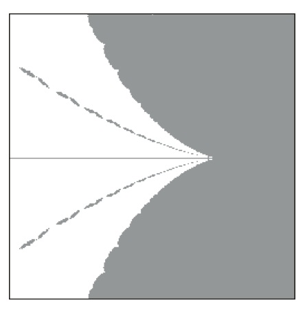
Figure 4: The linear slice $\mathcal{L}(\alpha)$ (gray part) for $\alpha=5.9+0i$; restricted to a neighborhood of $2$ whose width is about $0.2$. (The horizontal line thorough $2$ is the locus where the computer can not detect non-discreteness.)

Theorem 6.10.

There exists $\alpha\in\mathbb{C}$ such that $\mathcal{L}(\alpha)$ is not locally connected at $2\in\partial\mathcal{L}(\alpha)$; that is, $U\cap\mathcal{L}(\alpha)$ is disconnected for any sufficiently small neighborhood $U\subset\mathbb{C}$ of $2$.

Proof.

The homeomorphism $F:\mathcal{D}_{\mathrm{tr}}^{+}\to\mathcal{D}$ defined in section 5.3 induces a homeomorphism from

$$\mathcal{L}(\alpha)\cap\mathbb{C}_{+}=\{\beta\in\mathbb{C}:(\alpha,\beta)\in\mathcal{D}_{\mathrm{tr}}^{+}\}$$

to a slice

$$\{\zeta\in\hat{\mathbb{C}}:(i\alpha,\zeta)\in\mathcal{D}\}$$

of $\mathcal{D}$. Since $F(\alpha,2)=(i\alpha,\infty)$, to show that $\mathcal{L}(\alpha)$ is not locally connected at $2$ for some $\alpha$, it suffices to show that the set $\{\zeta\in\hat{\mathbb{C}}:(i\alpha,\zeta)\in\mathcal{D}\}$ is not locally connected at $\zeta=\infty$. We will show this by using the fact observed in [Br] that the vertical slice $\{\zeta\in\hat{\mathbb{C}}:(i\alpha,\zeta)\in\mathcal{A}\}$ of $\mathcal{A}$ is not locally connected at $\zeta=\infty$ for some $\alpha$.

From the argument of Bromberg in the proof of Theorem 4.15 in [Br], there exist $\mu\in\mathrm{int}(\mathcal{M})$, $\zeta\in\mathbb{C}$ with $\mathrm{Im}\,\zeta>0$, and $\epsilon>0$ such that $B_{\epsilon}(\mu,\zeta+2n)$ are contained in different connected components of

$$\{(\nu,z)\in\mathcal{A}:|\nu-\mu|<2\epsilon\}$$

for every integer $n$. By Theorem 4.3, we can take neighborhoods $U$, $W$ of $(\mu,\infty)$ in $\mathcal{A}$, $\mathcal{D}$, respectively, such that $\varphi=F\circ{\mathrm{Tr}}\circ\Phi:U\to W$ is a homeomorphism. We may assume that $U$ is of the form

$$U=\mathcal{A}\cap\{(\nu,z)\in\mathbb{C}^{2}:|\nu-\mu|<2\epsilon,|z|>K\}.$$

Then for all large $n$, $B_{\epsilon}(\mu,\zeta+2n)$ are contained in $U$, and thus contained in distinct connected components of $U$.

By choosing $\epsilon>0$ sufficiently small and $K>0$ sufficiently large, we see from Proposition 5.2 that $B_{\epsilon/2}(\mu,\zeta+2n)\subset\mathcal{D}$ for all large $n$. Therefore, $B_{\epsilon/2}(\mu,\zeta+2n)$ are contained in distinct connected components of $W$ for all large $n$. Since $W\subset\mathcal{D}$ is a neighborhood of $(\mu,\infty)$, we see that the set $\{\zeta\in\hat{\mathbb{C}}:(\mu,\zeta)\in\mathcal{D}\}$ is not locally connected at $\zeta=\infty$. Letting $\alpha=-i\mu$, we obtain the result. ∎

7 Complex Fenchel-Nielsen coordinates

In this section, we restate Theorems 6.6 and 6.8 in terms of the complex Fenchel-Nielsen coordinates. We begin with recalling the definition of the real Fenchel-Nielsen coordinates for Fuchsian representations.

Given $\lambda>0$, we define a representation $\eta_{\lambda}\in R(N,P)$ by

$$\eta_{\lambda}(a):=\frac{1}{\sinh(\lambda/2)}\left(\begin{array}[]{cc}\cosh(\lambda/2)&-1\\ -1&\cosh(\lambda/2)\end{array}\right),\quad\eta_{\lambda}(b):=\left(\begin{array}[]{cc}e^{\lambda/2}&0\\ 0&e^{-\lambda/2}\end{array}\right).$$

Then $\eta_{\lambda}(\pi_{1}(N))$ acts properly discontinuously on the upper-half plane ${\bf H}^{2}$, and hence is a Fuchsian group (see Figure 5, left). Note that $\eta_{\lambda}(a)$ fixes $-1,1$, $\eta_{\lambda}(b)$ fixes $0,\infty$, and thus the axes of $\eta_{\lambda}(a)$ and $\eta_{\lambda}(b)$ are perpendicular to each other. In addition, the complex length of $\eta_{\lambda}(b)$ is equal to $\lambda\in\mathbb{R}$.

Now we add a twisting parameter $\tau$. Given $(\lambda,\tau)\in\mathbb{R}_{+}\times\mathbb{R}$, we define a fuchsian representation $\eta_{\lambda,\tau}\in R(N,P)$ by

$$\eta_{\lambda,\tau}(a):=\left(\begin{array}[]{cc}e^{\tau/2}&0\\ 0&e^{-\tau/2}\end{array}\right)\eta_{\lambda}(a),\quad\eta_{\lambda,\tau}(b):=\eta_{\lambda}(b).$$

Note that the quotient surface ${\bf H}^{2}/\eta_{\lambda,\tau}(\pi_{1}(N))$ is obtained by cutting the surface ${\bf H}^{2}/\eta_{\lambda}(\pi_{1}(N))$ along the geodesic representative of $\eta_{\lambda}(b)$, twisting by hyperbolic length $\tau$ and re-glueing (see Figure 5, right).

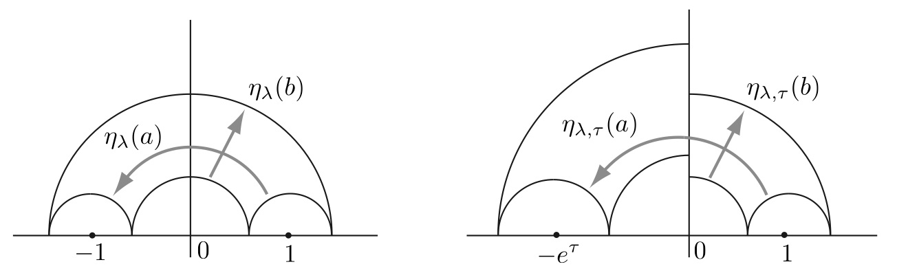
Figure 5: Fundamental domains of images of $\eta_{\lambda}$ (left) and $\eta_{\lambda,\tau}$ (right).

Now we obtain a map

$$FN:\mathbb{R}_{+}\times\mathbb{R}\to R(N,P)$$

defined by $(\lambda,\tau)\mapsto\eta_{\lambda,\tau}$. It is well-known that this map is a homeomorphism onto the space of Fuchsian representations. By allowing the parameters $\lambda,\tau$ to be complex numbers, we obtain a map

$$FN:(\mathbb{C}\setminus 2\pi i\mathbb{Z})\times\mathbb{C}\to R(N,P).$$

We say that $(\lambda,\tau)$ is the complex Fenchel-Nielsen coordinates of the representation $\eta_{\lambda,\tau}$. Note that if $\lambda\in\mathbb{R}$ and $\tau\in\mathbb{C}$, $\eta_{\lambda,\tau}$ is the complex earthquake of $\eta_{\lambda}$, see [Mc2]. It is known by Kourouniotis [Ko] and Tan [Ta] that there is an open subset of $(\mathbb{C}\setminus 2\pi i\mathbb{Z})\times\mathbb{C}$ containing $\mathbb{R}_{+}\times\mathbb{R}$ such that the map $FN$ induces a homeomorphism from this set onto the quasifuchsian space $MP(N,P)$.

Let

$$\mathcal{D}_{FN}:=\{(\lambda,\tau)\in(\mathbb{C}\setminus 2\pi i\mathbb{Z})\times\mathbb{C}:\eta_{\lambda,\tau}\in AH(N,P)\}.$$

Since we have

$${\mathrm{tr}}^{2}\eta_{\lambda,\tau}(a) = 4\coth^{2}\left(\frac{\lambda}{2}\right)\cosh^{2}\left(\frac{\tau}{2}\right),$$

$${\mathrm{tr}}^{2}\eta_{\lambda,\tau}(b) = 4\cosh^{2}\left(\frac{\lambda}{2}\right),$$

the map $\Theta:(\mathbb{C}\setminus 2\pi i\mathbb{Z})\times\mathbb{C}\to\mathbb{C}^{2}$ defined by

$$\Theta(\lambda,\tau):=\left(2\coth\left(\frac{\lambda}{2}\right)\cosh\left(\frac{\tau}{2}\right),2\cosh\left(\frac{\lambda}{2}\right)\right)$$

takes $\mathcal{D}_{FN}$ onto $\mathcal{D}_{\mathrm{tr}}$. For a given $\lambda\in\mathbb{C}\setminus 2\pi i\mathbb{Z}$, let

$$\widetilde{\mathcal{L}}(\lambda):=\{\tau\in\mathbb{C}:\eta_{\lambda,\tau}\in AH(N,P)\}.$$

We define a map $f_{\lambda}:\mathbb{C}\to\mathbb{C}$ by

$$f_{\lambda}(z):=2\coth\left(\frac{\lambda}{2}\right)\cosh\left(\frac{z}{2}\right)$$

so that we have $\Theta(\lambda,\tau)=(f_{\lambda}(\tau),2\cosh(\lambda/2))$. Then the map $f_{\lambda}$ takes $\widetilde{\mathcal{L}}(\lambda)$ onto $\mathcal{L}(\beta)$ where $\beta=2\cosh(\lambda/2)$. Note that $\widetilde{\mathcal{L}}(\lambda)$ is $\langle z+\lambda,z+2\pi i\rangle$-invariant, where the translation $z\mapsto z+\lambda$ corresponds to the Dehn twist about $b$.

We want to understand the shape of $\widetilde{\mathcal{L}}(\lambda)$ by using the Maskit slice $\mathcal{M}$ when $\lambda$ lies in $\mathbb{C}_{+}$ and is close to zero. To this end, we normalize $\widetilde{\mathcal{L}}(\lambda)$ so that the action of the Dehn twist about $b$ corresponds to the translation $z\mapsto z+2$. (Recall that the Maskit slice $\mathcal{M}$ has this property.) Let us define a map $g_{\lambda}:\mathbb{C}\to\mathbb{C}$ by

$$g_{\lambda}(z):=\frac{2}{\lambda}(z-\pi i)$$

and set

$$\widehat{\mathcal{L}}(\lambda):=g_{\lambda}(\widetilde{\mathcal{L}}(\lambda))$$

Then $\widehat{\mathcal{L}}(\lambda)$ is $\langle z+2,z+4\pi i/\lambda\rangle$-invariant and the map

$$h_{\lambda}(z):=f_{\lambda}\circ g_{\lambda}^{-1}(z)$$

takes zero to zero and $\widehat{\mathcal{L}}(\lambda)$ onto $\mathcal{L}(\beta)$, where $\beta=2\cosh(\lambda/2)$.

Since

$$h_{\lambda}(z) = 2\coth\left(\frac{\lambda}{2}\right)\cosh\left(\frac{\lambda z}{4}+\frac{\pi i}{2}\right)$$

$$= 2i\coth\left(\frac{\lambda}{2}\right)\sinh\left(\frac{\lambda z}{4}\right),$$

one can see that if $\lambda_{n}\to 0$ as $n\to\infty$, then $h_{\lambda_{n}}(z)\to iz$ uniformly on any compact subset of $\mathbb{C}$. Thus we obtain the following corollary of Theorems 6.6 and 6.8 (see Figure 6):

Corollary 7.1.

Suppose that $\lambda_{n}\in\mathbb{C}_{+},\lambda_{n}\to 0$ as $n\to\infty$.

1. If $\lambda_{n}\to 0$ horocyclically, then $\widehat{\mathcal{L}}(\lambda_{n})$ converge to $\mathcal{M}$ in the sense of Hausdorff, and $\mathrm{int}(\widehat{\mathcal{L}}(\lambda_{n}))$ converge to $\mathrm{int}(\mathcal{M})$ in the sense of Carathéodory.

2. Suppose that $\lambda_{n}\to 0$ tangentially. In addition we assume that there exist a sequence of integers $\{m_{n}\}_{n=1}^{\infty}$ such that the sequence $2\pi i/\lambda_{n}-m_{n}$ converges to some $\xi\in\mathbb{C}$ as $n\to\infty$. Then $\widehat{\mathcal{L}}(\lambda_{n})$ converge to $\mathcal{M}({2\xi})$ in the sense of Hausdorff, and $\mathrm{int}(\widehat{\mathcal{L}}(\lambda_{n}))$ converge to $\mathrm{int}(\mathcal{M}({2\xi}))$ in the sense of Carathéodory.

Proof.

The statement for Hausdorff convergence can be easily seen. The statement for Carathéodory convergence follows form Hausdorff convergence of the complements. ∎

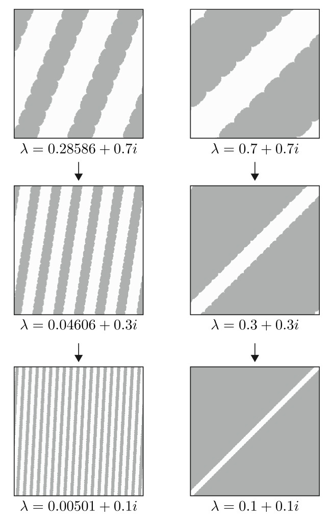
Figure 6: Computer-generated figure of $\widetilde{\mathcal{L}}(\lambda)$ (gray parts) for $\lambda$ close to $0$, restricted to the square of width $2\pi$ centered at $\pi i$. The left column corresponds to tangential convergence $\lambda\to 0$, where $\lambda$ are points on the circle $|z-1|=1$ whose imaginary part equal $0.7$ (top), $0.3$ (middle) and $0.1$ (bottom). The right column corresponds to horocyclic convergence $\lambda\to 0$, where $\lambda$ equal $0.7+0.7i$ (top), $0.3+0.3i$ (middle) and $0.1+0.1i$ (bottom).

References

- [AC] J. W. Anderson and R. D. Canary. Algebraic limits of Kleinian groups which rearrange the pages of a book. Invent. Math. 126 (1996), no. 2, 205–214.
- [BCM] J. .F. Brock, R. D. Canary and Y. N. Minsky, The classification of Kleinian surface groups, II: The ending lamination conjecture. Ann. of Math. (2) 176 (2012), no. 1, 1–149.
- [Br] K. W. Bromberg, The space of Kleinian punctured torus groups is not locally connected. Duke Math. J. 156 (2011), 387–427.
- [Bo] B. H. Bowditch, Markoff triples and quasi-Fuchsian groups. Proc. London Math. Soc. (3) 77 (1998), no. 3, 697–736.
- [Ca] R. D. Canary. Introductory Bumponomics: the topology of deformation spaces of hyperbolic 3-manifolds, in Teichmüller Theory and Moduli Problem, ed. by I. Biswas, R. Kulkarni and S. Mitra, Ramanujan Mathematical Society, 2010, 131-150.
- [Go] W. M. Goldman, Trace coordinates on Fricke spaces of some simple hyperbolic surfaces. Handbook of Teichmüller theory. Vol. II, 611–684, IRMA Lect. Math. Theor. Phys., 13, Eur. Math. Soc., Zürich, 2009.
- [It] K. Ito, Convergence and divergence of Kleinian punctured torus groups. Amer. J. Math. 134 (2012), 861–889.
- [Jø] T. Jørgensen. On discrete groups of Mobius transformations. Amer. J. Math. 98 (1976), no. 3, 739–749.
- [JK] T. Jørgensen and P. Klein, Algebraic convergence of finitely generated Kleinian groups. Quart. J. Math. Oxford Ser. (2) 33 (1982), no. 131, 325–332.
- [Ko] C. Kourouniotis, Complex length coordinates for quasi-Fuchsian groups. Mathematika 41 (1994), no. 1, 173–188.
- [KS] L. Keen and C. Series, Pleating coordinates for the Maskit embedding of the Teichmüller space of punctured tori. Topology 32 (1993), no. 4, 719–749.
- [KY] Y. Komori and Y. Yamashita, Linear slices of the quasi-Fuchsian space of punctured tori. Conform. Geom. Dyn. 16 (2012), 89–102.
- [Mag] A. D. Magid, Deformation spaces of Kleinian surface groups are not locally connected. Geometry & Topology 16 (2012), 1247–1320.
- [Mar] A. Marden, The geometry of finitely generated kleinian groups. Ann. of Math. (2) 99 (1974), 383–462.
- [Mc1] C. T. McMullen, Renormalization and 3-manifolds which fiber over the circle. Ann. of Math. Studies, 142. Princeton University Press, 1996.
- [Mc2] C. T. McMullen, Complex earthquakes and Teichmüller theory. J. Amer. Math. Soc. 11 (1998), no. 2, 283–320.
- [Mi] Y. N. Minsky, The classification of punctured-torus groups. Ann. of Math. (2) 149 (1999), no. 2, 559–626.
- [MSW] D. Mumford, C. Series and D. Wright, Indra’s pearls. The vision of Felix Klein. Cambridge University Press, New York, 2002.
- [PP] J. R. Parker and J. Parkkonen, Coordinates for quasi-Fuchsian punctured torus spaces. Epstein birthday schrift, (electronic), Geom. Topol. Monogr., 1 (1998), 451–478.
- [Su] D. Sullivan, Quasiconformal homeomorphisms and dynamics. II. Structural stability implies hyperbolicity for Kleinian groups. Acta Math. 155 (1985), no. 3-4, 243–260.
- [Ta] S. P. Tan, Complex Fenchel-Nielsen coordinates for quasi-Fuchsian structures. Internat. J. Math. 5 (1994), no. 2, 239–251.
- [Wr] D. J. Wright, The shape of the boundary of Maskit’s embedding of the Teichmüller space of once punctured tori. Preprint.