Ab-initio study of the effects induced by the electron–phonon scattering in carbon based nanostructures

Abstract

In this paper we investigate from first principles the effect of the electron–phonon interaction in two paradigmatic nanostructures: trans–polyacetylene  and polyethylene. We found that the strong electron–phonon interaction leads to the appearance of complex structures in the frequency dependent electronic self–energy. Those structures rule out any quasi–particle picture, and make the adiabatic and static approximations commonly used in the well–established Heine Allen Cardona (HAC) approach inadequate. We propose, instead, a fully ab-initio  dynamical formulation of the problem within the many-body perturbation theory  framework. The present dynamical theory reveals that the structures appearing in the electronic self–energy are connected to the existence of packets of correlated electron/phonon states. These states appear in the spectral functions even at $T=0\,K$, revealing the key role played by the zero point motion effect. We give a physical interpretation of these states by disclosing their internal composition by mapping the many body problem to the solution of an eigenvalue problem.

I Introduction

The electron–phonon (EP) coupling is well known to play a key role in several physical phenomena. For example it affects the renormalization of the electronic bandsAllen and Cardona (1983), the carriers mobility in organic devicesGosar and Choi (1966) or the position and intensity of Raman peaksAttaccalite et al. (2010). The EP coupling  is also the driving force that causes excitons dissociation at the donor/acceptor interface in organic photovoltaicTamura et al. (2008) and the transition to a superconducting phase in solidsMitsuhashi et al. (2010).

Despite the development of more powerful and efficient computational resources the calculation of the effects induced by the EP coupling in realistic materials remains a challenging task. In addition to the numerical difficulties, it has been assumed, for a long time, that this interaction can yield only minor corrections (of the order of meV) to the electronic levels. As a consequence the majority of the ab-initio  simulations of the electronic and optical properties of a wide class of materials are generally performed by keeping the atoms frozen in their crystallographic positions. It is actually well–known that phonons are atomic vibrations and, as a such, can be easily populated by increasing the temperature. This naive observation is de-facto used to associate the effect of the EP coupling to a temperature effect that vanishes as the temperature goes to zero. However this is not correct as the atoms posses an intrinsic spatial indetermination due to their quantum nature, that is independent on the temperature. These quantistic oscillations are taken into account by the EP coupling when $T\rightarrow 0$ in the shape of a zero–point–motion effect.

Many years agoCardona (2006) Heine, Allen and Cardona (HAC) pointed out the EP coupling can induce corrections of the electronic levels as large as those induced by the electronic correlation. As a consequence the generally accepted statement that the EP coupling always yields minor corrections was doomed to fail. Nowadays, the advent of more refined numerical techniques, has made possible to ground the HAC approach in a fully ab-initio  framework. This has been used to compute the gap renormalization in carbon–nanotubesCapaz et al. (2005), the finite temperature optical properties of semiconductors and insulators Marini , and to confirm a large zero–point renormalization ($615$ meV) of the band–gap of bulk diamond Giustino et al. (2010), previously calculated by Zollner using semi–empirical methodsZollner et al. (1992). These works are calling into question decades of results, by instilling the doubt that a solely electronic theory may be inadequate.

In this work we show that in nano–structures one of the approximations most commonly used in the electronic theories, the quasi–particle (QP) approximationLandau (1957), is seriously questioned by the effect of the EP coupling. Indeed in most electronic systems characterized by a moderate internal correlation, the electrons are believed to occupy well defined energy levels characterized by a precise energy, width and wave–function. The QP picture pictorially represents the effect of the correlation on these states as an electron–hole (in the case of electron–electron coupling) or electron–phonon (in the case of the EP coupling) pairs cloud which renormalizes the energy and the width of the electronic level, also reducing its effective electronic charge. The breakdown of the QP picture caused by the EP coupling  has been already predicted in the case of superconductors by Scalapino et al. Scalapino et al. (1966) and in complex metallic surfaces by Eiguren et al.Eiguren and Ambrosch-Draxl (2008). More recently we have shownCannuccia and Marini (2011) a strong renormalization of the electronic properties of diamond and trans-polyacetylene caused by the EP coupling in the zero temperature limit.

In this paper we will extend our previous workCannuccia and Marini (2011), by providing more methodological and technical details of the dynamical theory we have previously used. We will also apply the same method to another polymer, polyethylene, finding a severe breakdown of the QP picture. The analysis of the polyethylene  results will confirm and strengthen the general conclusions that we drew regarding the enormous impact of the electron–phonon coupling in carbon based nano–structures.

In sections II and III we will review the derivation of the fully frequency dependent self-energy by using the many-body perturbation theory. The HAC theory will be, then, found as a static and adiabatic limit of the dynamical theory. In section IV and V we will discuss how the structures appearing in the spectral functions of trans–polyacetylene  and polyethylene  rule out the basic assumptions of the HAC approach imposing the use of a fully dynamical theory. In section VI we will show how the problem can be mapped in the solution of a fictitious Hamiltonian that makes possible to define the polaronic states as complex electron–phonon packets. Finally, in the conclusions, we will point out as these results represent an important step forward in the simulation of nanostructures, with a wealth of possible implications in the development of more refined theories for the electronic and atomic dynamics.

II A dynamical approach to the electron–phonon problem

We start from the generic form of the total Hamiltonian of the system that we divide in electronic ($\widehat{H}_{el}$), atomic ($\widehat{H}_{at}$) and electron–atom part ($\widehat{H}_{el-at}$):

$$\widehat{H}=\widehat{H}_{el}+\widehat{H}_{at}+\widehat{H}_{el-at}.$$ (1)

The Hamiltonian $\widehat{H}$ admits both electronic and vibrational states that are coupled by $\widehat{H}_{el-at}$. In this work Density Functional Theory (DFT)R.M.Dreizler and E.K.U.Gross (1990) is used to calculate the eigenstates of $\overline{\widehat{H}}$, where we use the notation $\overline{O}$ to indicate a quantity or an operator that is evaluated with the atoms frozen in their equilibrium crystallographic positions. Similarly the vibrational states of the Hamiltonian $\widehat{H}$ are described, fully ab-initio, by using the well–known extension of DFT, the Density Functional Perturbation Theory (DFPT)Baroni et al. (2001); Gonze (1995). In DFPT the electronic correlations are embodied in a self–consistent mean potential $\widehat{V}_{scf}$ representing the total electronic potential which depends on the atomic positions ${\bf R}_{Is}\equiv{\bf R}_{I}+\tau_{s}$:

$$\widehat{H}_{el-at}=\int_{crystal}\,d{\bf r}\,\hat{\rho}\left({\bf r}\right)\widehat{V}_{scf}\left[\{{\bf R}\}\right]\left({\bf r}\right).$$ (2)

In the definition of ${\bf R}_{Is}$, $I$ and $s$ label the lattice cell (at position ${\bf R}_{I}$) and the atoms in the cell (at position $\tau_{s}$), respectively. In Eq.(2) $\rho$ is the electron density operator.

The aspect we are interested in this paper is how to properly include the modifications of the electronic levels induced by the atomic vibrations. In particular, by assuming the harmonic approximation for the phonons, we will develop a dynamical theory of the electronic dynamics. To this end we follow a purely diagrammatic approachMahan (1998) to present a short but accurate review of the derivation of the FanFan (1951) self–energy and of the much less known Debye–Waller (DW) correctionMarini and Cannuccia (2013).

If we now consider a configuration of lattice displacements $\hat{\bf u}_{Is}$, $\widehat{H}$ can be expressed as a Taylor expansion

$$\widehat{H}-\overline{\widehat{H}}=\sum_{Is\alpha}\overline{\frac{\partial\widehat{V}_{scf}\left[\{{\bf R}\}\right]\left({\bf r}\right)}{\partial{R_{Is\alpha}}}}\hat{u}_{Is\alpha}+\\ +\frac{1}{2}\sum_{Is\alpha,Js^{\prime}\beta}\overline{\frac{\partial^{2}\widehat{V}_{scf}\left[\{{\bf R}\}\right]\left({\bf r}\right)}{\partial{R_{Is\alpha}}\partial{R_{Js^{\prime}\beta}}}}\hat{u}_{Is\alpha}\hat{u}_{Js^{\prime}\beta},$$ (3)

where $\alpha$ and $\beta$ are the Cartesian coordinates.

The link with the perturbative expansion is readily done by transforming Eq. (3) from the space of the lattice displacements to the space of the canonical lattice vibrations by means of the identityMattuck (1976):

$$\hat{u}_{Is\alpha}=\sum_{{\bf q}\lambda}\left(2N_{q}M_{s}\omega_{{\bf q}\lambda}\right)^{-1/2}\xi_{\alpha}\left({\bf q}\lambda|s\right)e^{i{\bf q}\cdot\left({\bf R}_{I}+\tau_{s}\right)}\times\\ \times\left(\hat{b}^{\dagger}_{-{\bf q}\lambda}+\hat{b}_{{\bf q}\lambda}\right),$$ (4)

where $N_{q}$ is the number of cells (or, equivalently the number of q–points) used in the simulation and $M_{s}$ is the atomic mass of the $s$ atom in the unit cell. $\xi_{\alpha}\left({\bf q}\lambda|s\right)$ is the phonon polarization vector and $\hat{b}^{\dagger}_{-{\bf q}\lambda}$ and $\hat{b}_{{\bf q}\lambda}$ are the bosonic creation and annihilation operators.

By inserting Eq. (4) into Eq. (3) we get

$$\widehat{H}-\overline{\widehat{H}}=\frac{1}{\sqrt{N_{q}}}\sum_{{\bf k}nn^{{}^{\prime}}{\bf q}\lambda}g^{{\bf q}\lambda}_{nn^{\prime}{\bf k}}\hat{c}^{\dagger}_{n{\bf k}}\hat{c}_{n^{\prime}{\bf k}-{\bf q}}\left(\hat{b}^{\dagger}_{-{\bf q}\lambda}+\hat{b}_{{\bf q}\lambda}\right)+\\ +\frac{1}{N_{q}}\sum_{nn^{{}^{\prime}}{\bf k}}\sum_{{\bf q}\lambda,{\bf q}^{\prime}\lambda^{\prime}}\Lambda^{{\bf q}\lambda,{\bf q}^{\prime}\lambda^{\prime}}_{nn^{\prime}{\bf k}}c^{\dagger}_{n{\bf k}}c_{n^{\prime}{\bf k}-{\bf q}-{\bf q}^{\prime}}\times\\ \times\left(\hat{b}^{\dagger}_{-{\bf q}\lambda}+\hat{b}_{{\bf q}\lambda}\right)\left(\hat{b}^{\dagger}_{-{\bf q}^{\prime}\lambda^{\prime}}+\hat{b}_{{\bf q}^{\prime}\lambda^{\prime}}\right).$$ (5)

In Eq. (5) we have introduced the first–order ($g^{{\bf q}\lambda}_{n^{\prime}n{\bf k}}$) and the second–order ($\Lambda^{{\bf q}\lambda,{\bf q}^{\prime}\lambda^{\prime}}_{n^{\prime}n{\bf k}}$) electron–phonon matrix elements which will be shortly defined. To this purpose we rewrite $\widehat{V}_{scf}$ making explicit its dependence on the atomic positions:

$$\widehat{V}_{scf}\left[\{{\bf R}\}\right]\left({\bf r}\right)=\sum_{Is}\widehat{V}_{scf}\left({\bf r}-{\bf R}_{Is}\right).$$ (6)

From Eq. (6) it follows that the second order derivatives in the atomic positions are diagonal, $\frac{\partial^{2}}{\partial{\bf R}_{Is}\partial{\bf R}_{Js^{\prime}}}\widehat{V}_{scf}\left[\{{\bf R}\}\right]\left({\bf r}\right)\propto\delta_{IJ}\delta_{ss^{\prime}}\frac{\partial^{2}}{\partial{\bf R}^{2}_{Is}}\widehat{V}_{scf}\left[\{{\bf R}\}\right]\left({\bf r}\right)$.

By using Eq. (6) the summation on ${\bf R}_{I}$ appearing in Eq. (3) leads to the momentum conservation both in the first and second order terms. At the first order this leads to the definition of the electron–phonon matrix elements

$$g^{{\bf q}\lambda}_{nn^{\prime}{\bf k}}=\sum_{s\alpha}\left(2M_{s}\omega_{{\bf q}\lambda}\right)^{-1/2}e^{i{\bf q}\cdot\tau_{s}}\times\\ \times\langle n{\bf k}|\frac{\partial\widehat{V}_{scf}^{\left(s\right)}\left({\bf r}\right)}{\partial{R_{s\alpha}}}|n^{\prime}{\bf k}-{\bf q}\rangle\xi_{\alpha}\left({\bf q}\lambda|s\right),$$ (7)

We have also used the short form $R_{s\alpha}=\left.R_{Is\alpha}\right|_{I=0}$. A similar derivation can be followed to derive the 2^nd order term

$$\Lambda^{{\bf q}\lambda,{\bf q}^{\prime}\lambda^{\prime}}_{nn^{\prime}{\bf k}}=\frac{1}{2}\sum_{s}\sum_{\alpha,\beta}\frac{\xi^{*}_{\alpha}\left({\bf q}\lambda|s\right)\xi_{\beta}\left({\bf q}^{\prime}\lambda^{\prime}|s\right)}{2M_{s}\left(\omega_{{\bf q}\lambda}\omega_{{\bf q}^{\prime}\lambda^{\prime}}\right)^{1/2}}\times\\ \times\langle n{\bf k}|\frac{\partial^{2}\widehat{V}_{scf}^{\left(s\right)}\left({\bf r}\right)}{\partial{R_{s\alpha}}\partial{R_{s\beta}}}|n^{\prime}{\bf k}-{\bf q}-{\bf q}^{\prime}\rangle.$$ (8)

This second–order term is, in general, neglected as it is assumed to be small compared to the first–order term. Although this is correct at the level of the Hamiltonian it is not true anymore even at the lowest order of perturbation theory.

Indeed the different terms in the Taylor expansion of the Hamiltonian defined in Eq. (5) induce a wealth of diagrams of increasing complexity and order. If we restrict to the lowest non vanishing order we have two diagrams: the FanFan (1950) and the DW. These are presented by diagrams $(a)$ and $(b)$ in Fig. (1). In the same Figure two fourth order (in the displacements) diagrams, ($c$) and ($d$), are also showed. They are of the same order and, as the Fan and DW diagrams, they result from the perturbative treatment of the first order and second order terms in Eq. (5).

The actual calculation of the Fan and DW diagrams is straightforward. The Fan’s diagram is similar to the one generated by the electronic correlation in the so-called GW approximationStrinati et al. (1980), where the screened electronic interaction is replaced by a phonon propagator of wave vector ${\bf q}$ and branch $\lambda$Mahan (1998).

${\cal G}_{n{\bf k}}^{(0)}(\omega_{n})$

${\cal D}_{{\bf q}\lambda}^{(0)}(\omega_{j})$

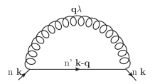
(a) 2^nd order $\Sigma^{Fan}$

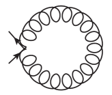
(b) 2^nd order $\Sigma^{DW}$

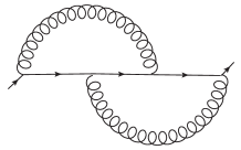
(c) 4^th order $\Sigma^{Fan}$

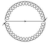
(d) 4^th order $\Sigma^{DW}$

Figure 1: The self-energy diagrams corresponding to the first and second order terms in the Taylor expansion of $\widehat{H}-\overline{\widehat{H}}$ (see Eq. (3)) treated at different orders of the perturbative expansion. For example the well–known Fan self-energy is formally obtained as a 2^nd order expansion of the first order term in Eq. (3). However the second term of Eq. (3), treated at first order gives the 2^nd order $\Sigma^{DW}$, that is of the same order of the Fan term and, consequently, cannot be neglected. The diagram (c) is obtained as a $4^{th}$ order expansion of the first order in Eq. (3) while (d) comes from the second term of Eq. (3) treated at the $2^{th}$ order.

Applying the finite temperature diagrammatic rules it is possible to define the Fan self-energy operator $\Sigma^{Fan}_{n{\bf k}}\left(i\omega_{i},T\right)$, recovering the expression originally evaluated by FanFan (1950):

$$\Sigma^{Fan}_{n{\bf k}}\left(i\omega_{i},T\right)=-\frac{1}{\beta}\frac{1}{N_{q}}\sum_{{\bf q}\lambda}\sum_{n^{\prime}}{\mid g^{{\bf q}\lambda}_{nn^{\prime}{\bf k}}\mid}^{2}\times\\ \times\sum^{+\infty}_{j=-\infty}D^{(0)}_{{\bf q}\lambda}\left(i\omega_{j}\right)G_{n^{\prime}{\bf k}-{\bf q}}^{(0)}\left(i\omega_{i}-i\omega_{j}\right),$$ (9)

where $\beta=\frac{1}{\mathit{K}T}$ ($\mathit{k}$ is the Boltzmann constant) and $T$ is the temperature of the phonon bath. By using the standard definitions of the electronic and the phononic Green’s functions: $G_{n^{\prime}{\bf k}}^{(0)}\left(i\omega_{i}\right)=\left(i\omega_{i}-\varepsilon_{n{\bf k}}+\mu\right)^{-1}$ (where $\mu$ is the chemical potential), $D_{{\bf q}\lambda}^{(0)}\left(i\omega_{j}\right)=\left(\left(i\omega_{j}-\omega_{{\bf q}\lambda}\right)^{-1}-\left(i\omega_{j}+\omega_{{\bf q}\lambda}\right)^{-1}\right)$, and summing over the Matsubara frequencies, we get the final expression for the Fan self–energy

$$\Sigma^{Fan}_{n{\bf k}}\left(i\omega,T\right)=\sum_{n^{\prime}{\bf q}\lambda}\frac{{\mid g^{{\bf q}\lambda}_{nn^{\prime}{\bf k}}\mid}^{2}}{N_{q}}\times\\ \times\left[\frac{N_{{\bf q}\lambda}\left(T\right)+1-f_{n^{\prime}{\bf k}-{\bf q}}}{i\omega-\varepsilon_{n^{\prime}{\bf k}-{\bf q}}-\omega_{{\bf q}\lambda}-i0^{+}}\right.+\\ +\left.\frac{N_{{\bf q}\lambda}\left(T\right)+f_{n^{\prime}{\bf k}-{\bf q}}}{i\omega-\varepsilon_{n^{\prime}{\bf k}-{\bf q}}+\omega_{{\bf q}\lambda}-i0^{+}}\right],$$ (10)

where $N_{{\bf q}\lambda}\left(T\right)$ is the Bose function distribution of the phonon mode $\left({\bf q},\lambda\right)$ at temperature $T$.

A similar expression can be derived for the frequency independent DW self–energy $\Sigma_{n{\bf k}}^{DW}$. This term comes from the equal time contractions of the $\left(\hat{b}^{\dagger}_{-{\bf q}\lambda}+\hat{b}_{{\bf q}\lambda}\right)\left(\hat{b}^{\dagger}_{-{\bf q}^{\prime}\lambda^{\prime}}+\hat{b}_{{\bf q}^{\prime}\lambda^{\prime}}\right)$ operators:

$$\langle\left(\hat{b}^{\dagger}_{-{\bf q}\lambda}+\hat{b}_{{\bf q}\lambda}\right)\left(\hat{b}^{\dagger}_{-{\bf q}^{\prime}\lambda^{\prime}}+\hat{b}_{{\bf q}^{\prime}\lambda^{\prime}}\right)\rangle=\\ \delta_{-{\bf q},{\bf q}^{\prime}}\delta_{\lambda,\lambda^{\prime}}\left[N_{{\bf q}^{\prime}\lambda}\left(T\right)+N_{{\bf q}\lambda}\left(T\right)+1\right].$$ (11)

The corresponding diagram ($b$) in Fig. 1 can be easily found to be

$$\Sigma^{DW}_{n{\bf k}}\left(T\right)=\frac{1}{N_{q}}\sum_{{\bf q}\lambda}\Lambda^{{\bf q}\lambda,-{\bf q}\lambda}_{nn{\bf k}}\left(2N_{{\bf q}\lambda}\left(T\right)+1\right).$$ (12)

Both the Fan and DW self-energy have been already derived previously in the framework of the Heine–Allen–Cardona (HAC) theory Allen and Heine (1976); Allen and Cardona (1983); Cardona (2006). The HAC approach is based on the static Rayleigh-Schrödinger perturbation theory. More precisely the $\hat{u}_{Is\alpha}$ are used as scalar variables on which a static perturbation theory is applied. As we will mention in Sec. III, the second–order derivatives appearing in the definition of the DW term can be rewritten in terms of the one–order derivatives by imposing the translational invariance of the correction to the electronic levels.

On the other hand the Fröhlich and the Holstein Hamiltonians usually neglect the DW term (diagram ($b$) in Fig. 1), even if it is of the same order of the Fan term.

The many body formulation represents the dynamical extension of the HAC approach, that is recovered from Eq. (10) by using $\omega\approx\varepsilon_{n{\bf k}}$ (the on–the–mass–shell (OMS) limit) and $\left|\varepsilon_{n{\bf k}}-\varepsilon_{n^{\prime}{\bf k}-{\bf q}}\right|\gg\omega_{{\bf q}\lambda}$ (the adiabatic limit) and by considering only the real part of the self–energy. It turns out, therefore, that in the HAC approach the temperature dependent change in the single–particle energies is given by

$$\Delta\varepsilon^{HAC}_{n{\bf k}}\left(T\right)=\Sigma^{DW}_{n{\bf k}}(T)+\sum_{n^{\prime}{\bf q}\lambda}\frac{{\mid g^{{\bf q}\lambda}_{nn^{\prime}{\bf k}}\mid}^{2}}{N_{q}}\frac{2N_{{\bf q}\lambda}\left(T\right)+1}{\varepsilon_{n{\bf k}}-\varepsilon_{n^{\prime}{\bf k}-{\bf q}}}.$$ (13)

The soundness of the HAC approach is then, from a MBPT perspective, connected to the validity of the on–the–mass–shell and of the adiabatic approximations. We will prove in the section IV that these approximations are not always well motivated. Dynamical and non–adiabatic corrections can be huge, such to invalidate the applicability of the HAC approach.

III Second order derivatives of $\widehat{V}_{scf}$ and the actual calculation of the Debye Waller self-energy

The general expression, Eq. (5) and Eq. (8) for the perturbed Hamiltonian requires the knowledge of the second–order gradients of the self–consistent potential

$$\Delta^{s\alpha\beta}_{n^{\prime}{\bf p},n{\bf k}}=\langle n^{\prime}{\bf p}|\frac{\partial^{2}\widehat{V}_{scf}^{\left(s\right)}\left({\bf r}\right)}{\partial{R_{s\alpha}}\partial{R_{s\beta}}}|n{\bf k}\rangle,$$ (14)

where ${\bf p}$ here replaces the ${\bf k}+{\bf q}+{\bf q}^{\prime}$ vector appearing in Eq. (5) and Eq. (8). These terms are extremely cumbersome to calculate and the task becomes easily prohibitive when higher orders are included. Their evaluation is, however, crucial because the ${\bf k}={\bf p}$ case is needed to calculate the lowest–order DW self-energy, while the finite momenta matrix element defines higher order diagrams (like diagram $(d)$ in Fig. (1)).

In the case of the simpler $\Sigma^{DW}_{n{\bf k}}$ (diagram $(b)$ in Fig. (1)) we know, from Eq. (8) and Eq. (14) that

$$\Lambda^{{\bf q}\lambda,-{\bf q}\lambda}_{nn{\bf k}}=\frac{1}{2}\sum_{s}\sum_{\alpha,\beta}\left(2M_{s}\omega_{{\bf q}\lambda}\right)^{-1}\times\\ \times\frac{\xi^{*}_{\alpha}\left({\bf q}\lambda|s\right)\xi_{\beta}\left(-{\bf q}\lambda|s\right)}{2M_{s}\omega_{{\bf q}\lambda}}\Delta^{s\alpha\beta}_{n{\bf k},n{\bf k}}.$$ (15)

In order to evaluate the $\Delta^{s\alpha\beta}_{n^{\prime}{\bf p},n{\bf k}}$ factors the HAC theory uses the fact that if all atoms were shifted by the same amount all physical quantities should not change. In other terms, being the $\Delta\varepsilon^{HAC}_{n{\bf k}}\left(T\right)$ an explicit functional of the atomic positions (Eq. (6)) that are treated classically, it is possible to impose the following translational invariance condition

$$\Delta\varepsilon^{HAC}_{n{\bf k}}\left[\{u_{Is\alpha}\}\right]\left(T\right)=\Delta\varepsilon^{HAC}_{n{\bf k}}\left[\{u_{Is\alpha}+d_{\alpha}\}\right]\left(T\right).$$ (16)

From this condition it follows that Allen and Heine (1976); Allen and Cardona (1983); Cardona (2006) in order to calculate $\Lambda^{{\bf q}\lambda,-{\bf q}\lambda}_{nn{\bf k}}$ that defines the DW self-energy (see Eq. (12)) only the matrix element $\Delta^{s\alpha\beta}_{n{\bf k},n{\bf k}}$ is needed. This can be rewritten as

$$\Delta^{s\alpha\beta}_{n{\bf k},n{\bf k}}=-\sum_{n^{\prime}\neq n}\frac{1}{\varepsilon_{n{\bf k}}-\varepsilon_{n^{\prime}{\bf k}}}\times\\ \times\left[\left(\sum_{s^{\prime}}\langle n{\bf k}|\frac{\partial\widehat{V}_{scf}^{\left(s^{\prime}\right)}\left({\bf r}\right)}{\partial{R_{s^{\prime}\alpha}}}|n^{\prime}{\bf k}\rangle\right)\langle n^{\prime}{\bf k}|\frac{\partial\widehat{V}_{scf}^{\left(s\right)}\left({\bf r}\right)}{\partial{R_{s\beta}}}|n{\bf k}\rangle\right.+\\ \left.+\langle n{\bf k}|\frac{\partial\widehat{V}_{scf}^{\left(s\right)}\left({\bf r}\right)}{\partial{R_{s\alpha}}}|n^{\prime}{\bf k}\rangle\left(\sum_{s^{\prime}}\langle n^{\prime}{\bf k}|\frac{\partial\widehat{V}_{scf}^{\left(s^{\prime}\right)}\left({\bf r}\right)}{\partial{R_{s^{\prime}\beta}}}|n{\bf k}\rangle\right)\right].$$ (17)

The condition given by Eq. (16) is, however, intrinsically ill–defined in the diagrammatic approach: the correction to the energy levels is a quantity obtained in fact, from the self-energy operator that, in turns, can be defined only when the displacement operators are quantized and a second quantized form of the Hamiltonian change (Eq. (5)) is introduced.

This inconsistency can be, indeed, cured in a fully MBPT framework Marini and Cannuccia (2013) but it requires to introduce the constant displacement vector $d_{\alpha}$ as an operator. This leads to the definition of new kinds of diagrams that will depend on powers of $d_{\alpha}$. By imposing that diagrams of the same order cancel each other it is possible to obtain a general expression for the matrix element $\Delta^{s\alpha\beta}_{n^{\prime}{\bf p},n{\bf k}}$.

As discussed by X. GonzeGonze et al. (2011), the local dependence on the atomic positions in Eq. (6) assumes that the electronic screening of the ionic potential, that defines $\widehat{V}_{scf}$, depends only smoothly on ${\bf R}_{Is}$. By taking fully into account this intrinsic dependence on the atomic positions a correction to the Debye–Waller term, named non–diagonal Debye–Waller correction, can be defined. This correction has been reported to be important for isolated molecules and atomsGonze et al. (2011). Its effect in solids and, more generally, in extended systems is expected to be weakened by the efficient screening properties.

IV Dynamical Self-Energy Effects beyond the Quasi Particle Approximation

In section II we showed that the HAC theory represents the static and adiabatic limit of the dynamical electron–phonon self-energy. The more suitable are the conditions of validity of the on–the–mass–shell and of the adiabatic approximations, the sounder is the applicability of the HAC approach from a MBPT perspective. We want to prove in this section that these approximations are not always well motivated and dynamical and non–adiabatic corrections to the HAC approach cannot be neglected a priori.

The HAC approach grounds on the concept of a well defined QP state: the charge carriers are assumed to be concentrated on electronic levels, being characterized by a well defined energy and wave-function. The QP concept can be firmly introduced in a many-body Green’s function theory Mahan (1998) where the definition embodies, at the same time, its limitations, as it will be clear in the following.

The fully interacting propagator can be written, for real energies $\omega$ in terms of the self-energy, (Eq. (9)) as

$$G_{n{\bf k}}\left(\omega,T\right)=\frac{1}{\omega-\varepsilon_{n{\bf k}}-\Sigma^{Fan}_{n{\bf k}}\left(\omega,T\right)-\Sigma^{DW}_{n{\bf k}}\left(T\right)}.$$ (18)

The rotation from the imaginary to the real axis has been easily performed by a Wick rotationMattuck (1976) as the energy dependence of the Fan self–energy is explicit. The single particle excitations are then the complex poles of Eq. (18)

$$\omega-\varepsilon_{n{\bf k}}-\Sigma^{DW}_{n{\bf k}}\left(T\right)-\Re\left[\Sigma^{Fan}_{n{\bf k}}\left(E_{n{\bf k}}\left(T\right),T\right)\right]+\\ -i\Im\left[\Sigma^{Fan}_{n{\bf k}}\left(E_{n{\bf k}}\left(T\right),T\right)\right]=0.$$ (19)

As it is clear from Eq. (19) a genuine QP state should have a zero line-width, that is a zero imaginary part of the self-energy. In practice this is never completely true. Nevertheless, when the frequency dependence of the self-energy is smooth Eq. (18) can be rewritten by using two simple and intuitive approximations: the OMS and the QP approximation. In the specific case of a constant and real self-energy (as in the HAC case) one can introduce the OMS approximation where the solution of Eq. (19) is given by

$$E_{n{\bf k}}\left(T\right)=\varepsilon_{n{\bf k}}+\Sigma^{DW}_{n{\bf k}}\left(T\right)+\Sigma^{Fan}_{n{\bf k}}\left(\varepsilon_{n{\bf k}},T\right).$$ (20)

We notice, from Eqs. (19) and (20), that $E_{n{\bf k}}\left(T\right)$ is complex. Even in the case where the self-energy is not constant, if the bare energy $\varepsilon_{n{\bf k}}$ is far from a pole of self-energy, then $\Sigma^{Fan}_{n{\bf k}}\left(\omega,T\right)$ can be Taylor expanded, up to the first order, around $\varepsilon_{n{\bf k}}$:

$$E_{n{\bf k}}\left(T\right)=\varepsilon_{n{\bf k}}+\Sigma^{DW}_{n{\bf k}}\left(T\right)+\Sigma^{Fan}_{n{\bf k}}\left(\varepsilon_{n{\bf k}},T\right)+\\ +\left.\frac{\partial\Sigma^{Fan}_{n{\bf k}}\left(\omega,T\right)}{\partial\omega}\right|_{\omega=\varepsilon_{n{\bf k}}}\left(E_{n{\bf k}}\left(T\right)-\varepsilon_{n{\bf k}}\right).$$ (21)

Eq. (21) corresponds to the QP approximation. The bare energy is then renormalized because of the virtual scatterings which are described by the real part of the self-energy. This renormalization is easily described by the solution of Eq. (21):

$$E_{n{\bf k}}\left(T\right)=\varepsilon_{n{\bf k}}+\\ +Z_{n{\bf k}}\left(T\right)\left[\Sigma^{Fan}_{n{\bf k}}\left(\varepsilon_{n{\bf k}},T\right)+\Sigma^{DW}_{n{\bf k}}\left(T\right)\right],$$ (22)

with $Z_{n{\bf k}}\left(T\right)=\left(1-\left.\frac{\partial\Sigma^{Fan}_{n{\bf k}}\left(\omega,T\right)}{\partial\omega}\right|_{\omega=\varepsilon_{n{\bf k}}}\right)^{-1}$ the renormalization factor. From Eq. (22) it is evident that $E_{n{\bf k}}$ is complex and its imaginary part $\Gamma_{n{\bf k}}\left(T\right)=\Im\left[E_{n{\bf k}}\left(T\right)\right]$, the QP line-width, is proportional to the $\Im\left[Z_{n{\bf k}}\left(T\right)\Sigma^{Fan}_{n{\bf k}}\left(\varepsilon_{n{\bf k}},T\right)\right]$. A small $\Gamma_{n{\bf k}}\left(T\right)$ indicates a stable QP, that slowly decays because of the real scatterings with the other particles and with the phonon modes. By assuming the QP approximation to be valid Eq. (18) can be re-written as $G_{n{\bf k}}\left(\omega,T\right)=Z_{n{\bf k}}\left(T\right)\left(\omega-E_{n{\bf k}}\left(T\right)\right)^{-1}$.

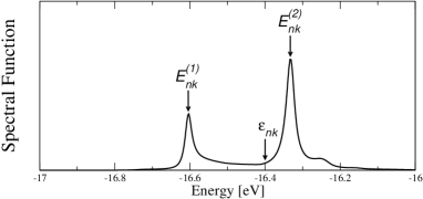
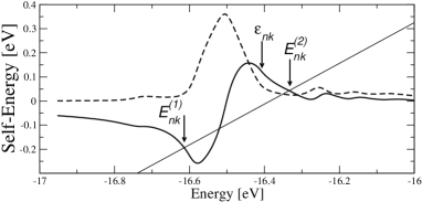
Figure 2: Trans–polyacetylene. Spectral function (upper frame) and self–energy (lower frame) corresponding to the state $\mid n=1,{\bf k}=\Gamma\rangle$. In the self–energy frame both the real (solid line) and imaginary (dashed line) parts are showed. The three arrows represent the bare electronic energy $\varepsilon_{n{\bf k}}$ and the two solutions ($E^{\left(1\right)}_{n{\bf k}}$,$E^{\left(2\right)}_{n{\bf k}}$) of Eq. (19). The thin solid straight line represents instead the function $\omega-\varepsilon_{n{\bf k}}-\Sigma_{n{\bf k}}^{DW}$. As the imaginary part of the self–energy shows a clear, intense and wide peak at around $-16.5$ eV (i.e. very close to $\varepsilon_{n{\bf k}}$) the real–part is dominated by a rapid oscillation that cannot be captured at all by the linearization of the energy dependence and causes the appearance of two solutions of Eq. (19).

Angle Resolved Photoemission Spectroscopy (ARPES) provides a definitive tool to verify if the QP approximation is accurate. If it existed a true QP should appear as a peak in the photoemission spectra with a Lorentzian lineshape. Indeed one finds that the spectral function (SF) $A_{n{\bf k}}\left(\omega,T\right)\equiv\pi^{-1}\mid\Im\left[G_{n{\bf k}}\left(\omega,T\right)\right]\mid$ is given, in the QP approximation and in the simple case of a purely real $Z_{n{\bf k}}$, by

$$A^{\left(qp\right)}_{n{\bf k}}\left(\omega,T\right)=\frac{Z_{n{\bf k}}\left(T\right)|\Gamma_{n{\bf k}}\left(T\right)|}{\pi\left[\left(\omega-\Re\left[E_{n{\bf k}}\left(T\right)\right]\right)^{2}+\Gamma^{2}_{n{\bf k}}\left(T\right)\right]}.$$ (23)

In this case the QP energy and width give the peak position and the spectral peak width. It is worth noticing that a complex value of $Z_{n{\bf k}}\left(T\right)$ would cause the spectral function to have an asymmetric lineshape.

The SF gives a physical interpretation and a clear validation of the QP approximation. Indeed $A^{\left(qp\right)}_{n{\bf k}}\left(\omega,T\right)$ is a probability function to find an electron in the state $n{\bf k}$ with energy $\omega$ and the total electronic charge associated to the QP state is $Z_{n{\bf k}}\left(T\right)$, that corresponds to the integral of $A^{\left(qp\right)}_{n{\bf k}}\left(\omega,T\right)$. The renormalization factor represents, therefore, the QP charge. When $Z_{n{\bf k}}\left(T\right)=1$ and $\Im\left[\Sigma_{n{\bf k}}(\varepsilon_{n{\bf k}},T)\right]\rightarrow 0$ the SF reduces to a delta function, the SF of a particle with energy $\Re\left[E_{n{\bf k}}\left(T\right)\right]$.

It is clear that a direct comparison of $A^{\left(qp\right)}_{n{\bf k}}\left(\omega,T\right)$ with the true SF corresponding to a given self–energy or with the ARPES lineshape provides the ultimate validation of the QP picture. A paradigmatic example that well explains the basic mechanism for the breakdown of the QP picture is given in Fig. 2 where the zero temperature SF for the $\mid n=1,{\bf k}=\Gamma\rangle$ state of trans–polyacetylene  is showed in the upper frame. It is clear that the SF of this state is far from being well represented by a Lorentzian lineshape. Indeed it is evident the appearance of two peaks at energies $E^{\left(1\right)}_{n{\bf k}}$ and $E^{\left(2\right)}_{n{\bf k}}$. These two peaks are the signature of a breakdown of the QP picture, because the existence condition of only one pole collecting most of the weight is not satisfied. We will come back on the physical interpretation of such structures in the next section. Nevertheless the origin of these two peaks is evident if we analyze the energy dependence of the imaginary and real parts of the corresponding self–energy, showed in the lower frame of the same figure. In this specific case the solution of Eq. (19) admits two roots as a consequence of the rapid oscillation of $\Re\left[\Sigma^{Fan}_{n{\bf k}}\left(\omega,T=0\right)\right]$ around $-16.5$ eV (the bare electronic energy of this state). This oscillation is, in turn, induced by an intense peak appearing in the $\Im\left[\Sigma^{Fan}_{n{\bf k}}\left(\omega,T=0\right)\right]$. We deduce that in this case a naive application of the QP approximation in form of a linearization of $\Sigma^{Fan}_{n{\bf k}}\left(\omega,T\right)$ (Eq. (21)) may produce a non physical energy dependence of the self–energy. As a consequence this leads to meaningless (negative or enormously large) values of $Z_{n{\bf k}}$.

In contrast to the case of purely electronic self–energies the QP approximation is known to lead to a too rough description of the electron–phonon spectral function for low–energy electrons in the homogeneous electron gas (jellium). As discussed by Engelsberg and Schrieffer Engelsberg and Schrieffer (1963) this failure, although not as dramatic as the one found in the present case, is linked to the mixing of electronic and phononic excitations. More precisely the authors identify three kind of excitations that appear as poles of the Green’s function when the energy of the electronic level is increased well above the Debye energy and the strength of the electron–phonon coupling is also increased. One is a purely QP state where the electron is dressed by a phonon cloud. The others lie in the continuum of electron–phonon pairs composed by clothed electrons and clothed phonons being excited, with a constant momentum sum.

V Breakdown of the Quasi Particle approximation: the case of trans–polyacetylene and polyethylene

In the previous section we showed that the structures appearing in the SF of trans–polyacetylene  rule out any description of the coupled electron–phonon system in terms of QPs. More importantly the rich structure of peaks appearing in the SF  described in Fig. 2 is not a fortuitous case. It is actually a general trend both in trans–polyacetylene  and in polyethylene. Indeed, in Figs. 3 and 4, the bare electronic band structure and the corresponding SFs   for a fixed ${\bf k}$ vector are shown in the upper frame. The position of the ${\bf k}$ vector in the Brillouin Zone (BZ) is represented by an horizontal line in the lower frame where the the valence bands of the two polymers are also reported.

In the upper frame of Figs. 3 and 4 there is also a sketch of the atomic structure of the polymers that helps to understand the main key differences among them. Both systems are linear polymers. Trans–polyacetylene  is a conjugated polymer where each carbon atom forms four nearest–neighbour bonds. Three of the four carbon valence electrons are in $sp^{2}$ hybridized orbitals and two of the $\sigma$-type bonds connect neighbour carbons along the one–dimensional backbone, while the third forms a bond with the hydrogen side group. Polyethylene , instead, is a $\sigma$-bonded, non–conjugated polymer. The atoms in the unit cell do not lie on a single plane like in trans–polyacetylene. The C atoms are sp³ hybridized and, as in the polyethylene  each C atom has four bonds.

From the upper panels of Figs. 3 and 4 it is evident that the EP interaction dramatically affects the spectral functions. The most striking aspect is that the SFs exhibit a multiplicity of structures. Although in some cases a single and strong peak can be observed the general trend is a very complex ensemble of peaks that makes impossible to apply the QP approximation. We will give a more formal and mathematical description of the internal structure of these peaks in the next section. Here we would like to underline some of their general aspects.

A remarkable aspect is that some SFs are so largely structured that they span a large energy range, even $3\,eV$ (see the $6^{th}$ band of polyethylene, Fig. 4). If they span a so large energy range, the SFs end up with overlapping each other in some cases (like the $4^{th}$ and $5^{th}$ band SFs in trans–polyacetylene). The crucial and straightforward consequence is that it turns out difficult to associate a single and well defined energy to the electron and, more importantly, different bands will energetically merge pointing to a non trivial mixing of the electronic states.

When a SF covers a large energy range, one peak may be distant in energy from the others more than the Debye energy ($0.4\,eV$ in trans–polyacetylene   and polyethylene). For this reason each peak can not be simply interpreted as a main QP peak plus a phonon replica. This point will be further discussed in Appendix A by using a two band model. Nevertheless it is reasonable to speculate that the formation of more than one peak suggests to reformulate the problem in a different framework where bare electrons are mixed with phonons, and not simply screened by phonons. Each peak appearing in the SF would be then identified by a mixed electron-phonon states. Since the many body   framework is not suitable to add information about the composition of the “new” mixed states, we will reformulate the problem in the next section by mapping the problem into and Hamiltonian representation.

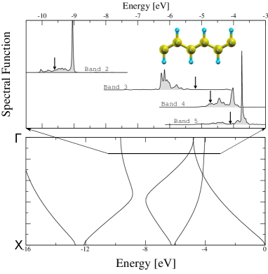
Figure 3: (color on line). The SFs of the last four occupied states in trans-polyacetylene (upper frame) are shown together with the DFT–LDA bands (lower frame). The horizontal line in the bands frame represents the position of the k–point and the energy range along which the SFs are displayed. The vertical arrows in the upper frame represents the energy position of the unperturbed DFT levels. Since these states correspond to in plane orbitals they are strongly affected by the in plane atomic vibrations. The result is that the bare electronic levels are split in several polaronic states.

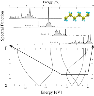
Figure 4: (color on line). Like in Fig.(3) in the polyethylene  case.

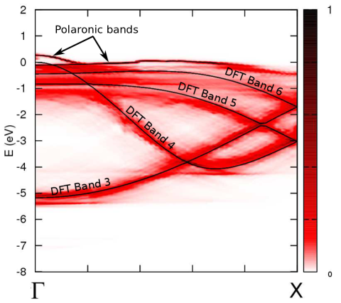
Figure 5: (color on line). Two dimensional plot of the spectral functions $\Delta Z_{n{\bf k}}(\omega)$ for polyethylene in the last four occupied bands region. The DFT and the polaronic bands are opportunely labeled. In general the electronic levels acquire a large energy indetermination if compared to the DFT bands represented by solid black lines. The EP interaction moves up of about $300$ meV the last two occupied bands leading to an increase of the band width. Moreover the 6^th band near the $X$ point shows a large energy indetermination that makes it almost disappearing.

A global view of the effect of the ZPM on the electronic structure of polyethylene  is given in Fig. 5 in the energy range of the last 4 occupied valence bands. The DFT electronic bands are drawn as a reference of the electronic band structure before switching on the EP interaction.

By defining $\Delta Z_{n{\bf k}}\left(\omega\right)\equiv A_{n{\bf k}}\left(\omega\right)\Delta\omega$ the probability to find an electron $\mid n{\bf k}\rangle$ in the small energy range $\Delta\omega=50\,meV$, we made a bidimensional representation of the probability amplitude. This is showed in Fig. 5 by using a colored scale that goes from white (the less intense peak), to black (the most intense one). As a consequence this picture gathers all the information about the energy range covered by the SFs  and the intensity of all peaks. In particular we observe that the $6^{th}$ band of polyethylene  moves up close to $\Gamma$-point and then the electron completely disappears.

The resulting zero point renormalization of the gap at $\Gamma$ point of polyethylene  is $280meV$, larger than the trans-polyacetylene case Cannuccia and Marini (2011). Such a difference is ascribed to the peculiar shape of the trans–polyacetylene  orbital at the $X$ point whose $\pi$ character corresponds to states perpendicular to the polymer axis. Thus they feel less the effect of the in-plane vibrations. On the other hand for polyethylene  at $\Gamma$, the electrons are localized along the $C-C$ bond, where the zero point motion effect of the electronic gap is sizable. For what concerns the deeper states far from the gap, the effect of the electron-phonon coupling is equally strong. In fact as they are in plane orbitals they are directly affected by in plane atomic vibrations.

We also observe that each band has a different energy width which evolves in different manners moving from $\Gamma$ to $X$. An increasing of the bandwidth is normally associated to a consequent increase of the delocalization of the orbitals. This fact can be used link the effect of the EP coupling to a increased electronic mobility mediated by the polaronic states.

In the next section we will go beyond this picture by introducing a general framework to link the poles of the electron–phonon Green’s functions to coupled packets of electron–phonon pairs.

VI Internal structure of the polaronic states via an Hamiltonian representation

In order to gain more insight into the complex structures that appear in the SFs of both trans–polyacetylene  and polyethylene  we propose, in this section, a mapping of the Many–Body problem into an equivalent Hamiltonian representation. In this representation the poles of the SF will appear as eigenvalues of a fictitious el–ph Hamiltonian. When this is solved in a specific restricted sub–space of the entire Fock space, it will reproduce the same SF obtained by solving the Dyson equation within the Fan and Debye–Waller approximations for the self–energy.

In order to show this we start by rewriting the SF  by using the well–known Lehmann representationMahan (1998):

$$A_{n{\bf k}}\left(\omega,T\right)=\sum_{I{\bf k}}{\mid\langle\Psi_{0}\mid c^{\dagger}_{n{\bf k}}\mid I{\bf k}\left(T\right)\rangle\mid}^{2}\delta\left(\omega-E_{I{\bf k}}\left(T\right)\right),$$ (24)

where $\mid I{\bf k}\left(T\right)\rangle$ are the true eigenstates of the system with energy $E_{I{\bf k}}\left(T\right)$ which, in turns, represent the true and real poles of the GF. As our initial Hamiltonian, Eq. (1), is composed of electrons and phonons the states $\mid I{\bf k}\left(T\right)\rangle$ live an extended Fock space composed of electrons and phonons.

In the QP approximation the distribution of peaks appearing in Eq. (24) is approximated with a Lorentzian distribution centered at the QP energy with a width equal to the QP line-width. Thus, Eq. (24) already underlines that the origin of the multiple poles in the SFs  shown in Fig. 3 and Fig. 4 is connected to the existence of more than one intense state $\mid I{\bf k}\rangle$ belonging to the same state $\mid n{\bf k}\rangle$.

Now we assume that Eq. (24) remains valid also when the exact self–energy is approximated by the Fan and Debye–Waller terms. And, in order to link the states $\mid I{\bf k}\left(T\right)\rangle$ to an Hamiltonian problem we start rewriting Eq. (1) in second quantization:

$$\widehat{H}=\widehat{H}_{el}+\widehat{H}_{ph}+\widehat{H}_{el-ph},$$ (25)

where $\widehat{H}_{el}$ is the electronic Hamiltonian, $\widehat{H}_{ph}$ is the independent phonons Hamiltonian and $\widehat{H}_{el-ph}$ is the EP interaction Hamiltonian. The last three terms, written in the second quantization, read

$$\widehat{H}_{el}=\sum_{n{\bf k}}\tilde{\varepsilon}_{n{\bf k}}c^{\dagger}_{n{\bf k}}c_{n{\bf k}},$$ (26)

$$\widehat{H}_{ph}=\sum_{{\bf q},\lambda}\omega_{{\bf q}\lambda}(b^{\dagger}_{{\bf q}\lambda}\hat{b}_{{\bf q}\lambda}+\frac{1}{2}),$$ (26^′)

$$\widehat{H}_{el-ph}=\frac{1}{N_{q}}\sum_{\begin{subarray}{c}n,n^{\prime},{\bf k},\\ {\bf q},\lambda\end{subarray}}{g^{{\bf q},\lambda}_{nn^{\prime}{\bf k}}c^{\dagger}_{n{\bf k}}c_{n^{\prime}{\bf k}-{\bf q}}(b^{\dagger}_{-{\bf q}\lambda}+b_{{\bf q}\lambda})}.$$ (26^′′)

In Eq. (26) $\tilde{\varepsilon}_{n{\bf k}}$ is a single particle energy that we will shortly define. $c^{\dagger}_{n{\bf k}}$ is the creation and $c_{n^{\prime}{\bf k}-{\bf q}}$ is the annihilation electronic operators, $b^{\dagger}_{{\bf q}\lambda}$ and $\hat{b}_{{\bf q}\lambda}$ are the creation and annihilation operators for phonons with energy $\omega_{{\bf q}\lambda}$ and wave vector ${\bf q}$. $g^{{\bf q},\lambda}_{nn^{\prime}{\bf k}}$ are the EP coupling matrix elements (see Eq. (7)).

We want now to use Eqs. (26) to calculate the states $|I{\bf k}\left(T\right)\rangle$. To this end we note, from the (a) frame of Fig.1, that the Fan self-energy makes an initial state $|n{\bf k}\rangle$ to scatter with a phonon state $|{\bf q}\lambda\rangle$, with population $N_{{\bf q}\lambda}\pm 1$, in a final state $|n^{\prime}{\bf k}-{\bf q}\rangle$. Only one phonon is exchanged and in the self–energy loop the intermediate states are the composite pairs $\mid n^{\prime}{\bf k}-{\bf q}\rangle\otimes\mid N_{{\bf q}\lambda}\pm 1\rangle$ with energy $\varepsilon_{n^{\prime}{\bf k}-{\bf q}}\pm\omega_{{\bf q}\lambda}$. This energy, indeed, appears in the denominator of Eq. (10).

Physically this means that, if we introduce the general state product of an electronic and phononic part $\mid n^{\prime}{\bf k-q}\rangle\otimes\mid N_{{\bf q}\lambda}\pm 1\rangle$, the intermediate states of the self–energy are all possible combinations with different ${\bf q}$ and $\lambda$. It follows that we can guess, at a given temperature,

$$\mid I{{\bf k}}\left(T\right)\rangle=\sum_{n}A^{I}_{n{\bf k}}\left(T\right)\mid n{\bf k}\rangle+\\ +\sum_{n^{\prime}{\bf q}\lambda}B^{I\lambda}_{n^{\prime}{\bf k}-{\bf q}}\left(T\right)\mid n^{\prime}{\bf k-q}\rangle\otimes\mid N_{{\bf q}\lambda}\left(T\right)\pm 1\rangle.$$ (27)

The coefficients $A^{I}$ and $B^{I\lambda}$ can be found by diagonalizing Eq. (25) in the space of electron–phonon states spanned by the definition given in Eq. (27). More precisely, in order to expand the matrix form of Eq. (25) we notice that, due to Eq. (27) the basis set will be composed of the following elements

$$\mid n{\bf k}\rangle\mid N_{{\bf q}\lambda}\rangle,\,\,\mid n{\bf k}-{\bf q}\rangle\mid N_{{\bf q}\lambda}\pm 1\rangle.$$ (28)

At zero temperature the basis set is reduced to

$$\mid n{\bf k}\rangle\mid 0_{ph}\rangle,\,\,\mid n{\bf k}-{\bf q}\rangle\mid 1_{{\bf q}\lambda}\rangle,$$ (29)

and it reflects the fact that at $T=0\,K$ there are no phonons in the ground state. In this restricted basis the Hamiltonian reads

$$\widehat{H}=\begin{bmatrix}\ddots&&&&\\ &\tilde{\varepsilon}_{n{\bf k}}\delta_{nn^{\prime}}&&H^{ep}_{nn^{\prime}{\bf q}\lambda}&\\ &&\ddots&&\\ &(H^{ep}_{nn^{\prime}{\bf q}\lambda})^{\dagger}&&\tilde{\varepsilon}_{n{\bf k}-{\bf q}}\delta_{nn^{\prime}}+\omega_{{\bf q}\lambda}\delta_{{\bf q}{\bf q}^{\prime}}\delta_{\lambda\lambda^{\prime}}&\\ &&&&\ddots\\ \end{bmatrix}.$$ (30)

The fact that $\hat{H}_{el-ph}$ is Hermitian makes also $\hat{H}$ Hermitian. The equivalence of Eq. (24) with the spectral function calculated in Sec.IV is obtained by imposing $\tilde{\varepsilon}_{n{\bf k}}=\varepsilon_{n{\bf k}}+\Sigma^{DW}_{n{\bf k}}$. This equivalence is proved analytically, in the zero temperature limit, in Appendix A for a simple two–levels model.

From Eq. (30) we also note that the number of states $\mid I{{\bf k}}\left(T\right)\rangle$ is equal to the dimension of the matrix and it is obtained by multiplying the number of electronic bands times the number of ${\bf q}$ vectors times the number of phononic branches, $\lambda$. As a consequence the number of states $\mid I{{\bf k}}\left(T\right)\rangle$ is larger than that of $\widehat{H}_{el}$. This confirms the fact that, in Eq. (24), the states $|I{\bf k}\left(T\right)\rangle$ form a continuum that, in the QP approximation, dresses the bare electronic state. This dressing is, de–facto, represented by a cloud of mixed electron–phonon states surrounding the QP energy with a Lorentzian distribution.

The Hamiltonian $\widehat{H}$ (Eq. (30)) is diagonalized for trans–polyacetylene  including $30$ electronic bands, $10\,{\bf q}$-vectors and $12$ phonon branches. Since the Hamiltonian is written on a complete basis, the coefficients $A^{I}_{n{\bf k}}$ and $B^{I\lambda}_{n^{\prime}{\bf k}-{\bf q}}$ satisfy the following condition

$$\sum_{n}\mid A^{I}_{n{\bf k}}\mid^{2}+\sum_{n^{\prime}{\bf q}\lambda}\mid B^{I\lambda}_{n^{\prime}{\bf k}-{\bf q}}\mid^{2}=1,$$ (31)

which ensures that the spectral function $A_{n{\bf k}}\left(\omega,T\right)$ is correctly normalized to 1 when integrated over all frequencies. Once the eigenstates $\mid I{{\bf k}}\rangle$ and the eigenvalues $E_{I{{\bf k}}}$ are known, the SF  can be calculated according to Eq. (24) and all the peaks appearing in the SFs  of state $\mid n{\bf k}\rangle$, are unambiguously labeled with a particular $\mid I{{\bf k}}\rangle$ state, having $\mid n{\bf k}\rangle$ as the pure electronic component. Let us consider the $\mid n=4,{\bf k}=0.2(\frac{2\pi}{a},0,0)\rangle$ state of trans–polyacetylene  as an example. In Fig. 6 it is shown the corresponding zero temperature SF.

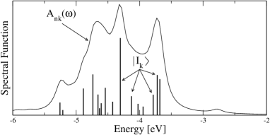
Figure 6: Trans–polyacetylene. The SF  of the state $\mid n=4,{\bf k}=0.2(\frac{2\pi}{a},0,0)\rangle$ is decomposed in polaronic states, each labeled by $\mid I{\bf k}\rangle$. Several structures appear thus ruling out the QP approximation.

The poles and the corresponding residuals are indicated in Fig. 6 by bars with different heights. The residuals are given by $\mid A^{I}_{n{\bf k}}\mid^{2}$, that is the probability to find the polaronic state in the pure electronic $\mid n{\bf k}\rangle$ state. This reminds the physical meaning of the $Z_{n{\bf k}}$ factors, and we use this similarity to define $Z^{I}_{n{\bf k}}=\mid A^{I}_{n{\bf k}}\mid^{2}$. Nevertheless from Eq. (27) it is evident that the smaller the $Z^{I}_{n{\bf k}}$ is, the less the polaronic state can be assimilated to an electron. It means that the mixed EP contribution in Eq. (27) indeed weights the most. In the case of Fig. 6 the $\mid A^{I}_{n{\bf k}}\mid^{2}$ can even be as small as 0.2.

These small values of $Z^{I}_{n{\bf k}}$ represent a general trend. In Fig. 7 $Z^{I}_{n{\bf k}}$ is plotted as a function of the polaronic eigenvalues.

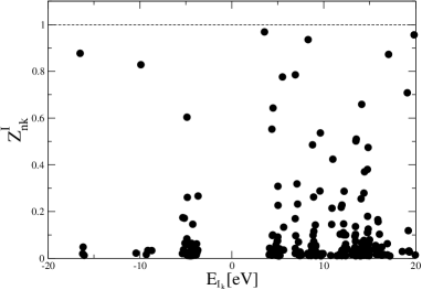
Figure 7: Trans–polyacetylene. The projection of the polaronic states over the corresponding pure electronic state, $Z^{I}_{n{\bf k}}$ is shown. The dashed line represents $Z^{I}_{n{\bf k}}$ of a pure electron state as a reference value.

It can be noted that only few polaronic states have $Z^{I}_{n{\bf k}}\simeq 1$. Most of all are below $0.5$, instead. It means that the mixed EP part of the eigenstate, shown in Eq. (27), plays a dominant role.

A small value of $Z^{I}_{n{\bf k}}$ points to a non trivial physical property of the polaronic states. When $Z^{I}_{n{\bf k}}\rightarrow 0$ it is evident that only the mixed terms in the sum, where the electrons and the phonons appear together, are non zero. This means that the electrons cannot move in the system alone, even if dressed by an electron–phonon cloud, but need to build up true bound electron–phonon states. This is a clear fingerprint of the breakdown of the QP approximation.

The generic definition of the polaronic state, Eq. (27), allows to calculate the mean value of any observable that lives in the mixed electron–phonon space. For example we can evaluate the matrix elements of the atomic indetermination operator as follows

$$u^{2}_{\alpha I{\bf k}s}\equiv\langle I{\bf k}\mid u^{2}_{\alpha,s}\mid I{\bf k}\rangle=\\ \sum_{{\bf q}\lambda}\left(\frac{1}{2N_{q}\omega_{{\bf q}\lambda}M_{s}}\right)\varepsilon_{\alpha}\left({\bf q}\lambda/s\right)\varepsilon^{\ast}_{\alpha}\left({\bf q}\lambda/s\right)\times\\ \times\left[\sum_{n}\mid A^{I}_{n{\bf k}}\mid^{2}+3\sum_{n^{\prime}}\mid B^{I\lambda}_{n^{\prime}{\bf k}-{\bf q}}\mid^{2}\right].$$ (32)

By using these $u^{2}_{\alpha I{\bf k}s}$ we can associate an average quantum size to the atoms.

	Trans–polyacetylene		polyethylene
	$C$	$H$	$C$	$H$
	$a.u.$	$a.u.$	$a.u.$	$a.u.$
$\hat{x}$	$0.18$	$0.55$	$0.1$	$0.32$
$\hat{y}$	$0.13$	$0.36$	$0.07$	$0.21$
$\hat{z}$	$0.11$	$0.56$	$0.07$	$0.34$

Table 1: Atomic amplitudes obtained by evaluating the matrix elements of operator $\sqrt{\mathbf{u}^{2}_{I{\bf k}s}}$. Because of its smaller mass the hydrogen quantum atomic size is three times larger than the carbon atom one. Nevertheless the constraint imposed by the different geometries makes the deviation of the two polymers appreciably different.

The values for the $C$ and $H$ species, calculated by Eq. (32), are shown in Tab. 1. These values point to the fact that the atoms acquire an indetermination larger along the polymer axis. Since $H$ is lighter than $C$ the atomic quantum size is larger. The different constraint created by the geometries is the cause of the different $\sqrt{u^{2}_{\alpha I{\bf k}s}}$ values between the two polymers.

The values of the atomic indetermination suggest that electrons and phonons exert a cooperative effect on each other. The charge density spreads all along the polymer, while the atoms squeeze along $\hat{y}$ and $\hat{z}$ directions, widening along $\hat{x}$. This cooperation can cause, for example, an enhancement of the mobility, opening therefore new perspectives for future investigations and applications of polymers.

VII Conclusions

In this work we have shown that the Heine–Allen–Cardona approach suffers of some severe limitations when applied to predict the zero temperature energy correction in low dimensional systems. We extensively describe a fully dynamical extension of the Heine–Allen–Cardona approach to show that the zero point motion effect severely questions the reliability of the QP picture in trans-polyacetylene and polyethylene.

The single particle spectral functions, indeed, exhibit multiple structures at $T=0\,K$. The formation of additional structures caused by the strong electron–phonon interaction is interpreted in terms of composed electron–phonon states, what we call in this work polaronic states. These states are precisely defined by mapping the structures of the Many–Body spectral functions into the solution of an eigenvalue problem.

Thanks to this important mapping the non perturbative nature of the polaronic states appears as a coherent superposition of electron–phonon pairs. And the cooperative dynamics between electrons and atoms in these states rules out any description in terms of bare atoms and quasiparticles.

The resulting coupled electronic and atomic dynamics pave the way for new investigations in polymers and more in general in low dimensional nanostructures. The cooperative dynamics of electrons and phonons in the polaronic states can have potential physical implications, as for example, an enhancement of the electronic mobility.

More generally the breakdown of the quasiparticle picture imposes a critical analysis of the previous results obtained using purely electronic theories.

Appendix A A two–levels model to verify the Hamiltonian representation

In Sec.VI we have given physical arguments to support the choice of a specific limited Fock space where the Hamiltonian problem is solved. These arguments were guided by the final goal of introducing an Hamiltonian representation that gives exactly the Green’s functions corresponding to the Fan approximation for the self–energy. To better investigate and confirm this ansatz let us consider two levels of energies $\varepsilon_{i}=0,E$ coupled to a phonon of energy $\omega_{0}$ at $T=0\,K$.

Eqs. (25-30) thus reduce to a simple expression for the Hamiltonian of this system

$$H=\sum_{i=1}^{2}\epsilon_{i}c^{\dagger}_{i}c_{i}+\omega_{0}b^{\dagger}_{0}b_{0}+\sum_{\begin{subarray}{c}i=1,2\\ j=1,2\\ i\neq j\end{subarray}}gc^{\dagger}_{j}c_{i}(b^{\dagger}_{0}+b_{0}).$$ (33)

As discussed in Sec.VI we consider for the finite basis the following ansatz:

$$\mid 1\rangle\mid 0_{ph}\rangle,\mid 2\rangle\mid 0_{ph}\rangle,$$ (34)

$$\mid 1\rangle\mid 1_{ph}\rangle,\mid 2\rangle\mid 1_{ph}\rangle,$$ (35)

where by $\mid i\rangle$ we mean an electron in the level $i^{th}$. The dimension of the Hamiltonian matrix is then given by multiplying 2 bands $\times\,1\,{\bf q}$ point $\times\,1$ phonon branch, resulting in a $4\times 4$ matrix

$${\mathcal{H}}=\left(\begin{array}[]{cccc}0&0&0&g\\ 0&E&g&0\\ 0&g&\omega_{0}&0\\ g&0&0&E+\omega_{0}\end{array}\right),$$ (40)

which can be diagonalized in two blocks, obtaining the following four energy levels

$$E_{1}=\frac{E+\omega_{0}+\sqrt{(E+\omega_{0})^{2}+4g^{2}}}{2},$$ (41)

$$E_{2}=\frac{E+\omega_{0}-\sqrt{(E+\omega_{0})^{2}+4g^{2}}}{2},$$ (42)

$$E_{3}=\frac{E+\omega_{0}+\sqrt{(E-\omega_{0})^{2}+4g^{2}}}{2},$$ (43)

$$E_{4}=\frac{E+\omega_{0}-\sqrt{(E-\omega_{0})^{2}+4g^{2}}}{2}.$$ (44)

The corresponding four eigenvectors are

$$\mid I_{1}\rangle=\frac{1}{N_{1}}\left(\frac{g}{E_{1}},\,0\,,0,\,1\right),$$ (45)

$$\mid I_{2}\rangle=\frac{1}{N_{2}}\left(1,\,0\,,0,-\frac{g}{E_{1}}\right),$$ (46)

$$\mid I_{3}\rangle=\frac{1}{N_{3}}\left(0,\,1,\,-\frac{g}{\omega_{0}-E_{3}},\,0\right),$$ (47)

$$\mid I_{4}\rangle=\frac{1}{N_{4}}\left(0,\frac{g}{\omega_{0}-E_{3}},\,1\,,0\right),$$ (48)

where $N_{i}$ are the normalization factors, with $N_{1}=N_{2}$ and $N_{3}=N_{4}$.

These are the needed ingredients to calculate the Green’s functions  as matrix element of the resolvent

$${\cal{G}}_{i}(\omega)=\langle vac\mid c_{1}\,\frac{1}{\omega-H}\,c^{+}_{1}\mid vac\rangle,$$ (49)

where $\mid vac\rangle$ is the vacuum of phonons and electrons. Expanding in eigenstates of the system, Eq. (49) becomes

$${\cal{G}}_{i}(\omega) = \sum_{j=1}^{4}\langle vac\mid c_{i}\,\frac{1}{\omega-H}\mid I_{j}\rangle\langle I_{j}\mid c^{+}_{i}\mid vac\rangle$$ (50)

$$= \sum_{j=1}^{4}{\mid\langle vac\mid c_{i}\mid I_{j}\rangle\mid}^{2}\frac{1}{\omega-E_{j}}.$$

In order to show that the SFs  calculated from Eq. (50) are equivalent to the ones obtained in the MB approach, the Green’s function   for the $1^{st}$ state is evaluated from Eq. (50) as follows

$${\cal{G}}_{1}(\omega)=\frac{1}{E_{1}-E_{2}}\left[\frac{-E_{2}}{\omega-E_{1}}+\frac{E_{1}}{\omega-E_{2}}\right].$$ (51)

On the other hand the Fan approximation for the self-energy, Eq. (10), in this test case reduces to

$$\Sigma^{Fan}_{1}(\omega)=g^{2}\left[\frac{N(\omega_{0})+1-f_{2}}{\omega-E-\omega_{0}-i0^{+}}+\right.\\ \left.\frac{N(\omega_{0})+f_{2}}{\omega-E+\omega_{0}-i0^{+}}\right].$$ (52)

At zero temperature the Bose occupation factors vanish. The Fermi occupation factor $f_{2}$ is zero because the level is empty and Eq. (52) becomes

$${\cal{G}}_{1}(\omega)=\frac{1}{\omega-g^{2}\left[\frac{1}{\omega-E-\omega_{0}}\right]-i0^{+}}.$$ (53)

The poles of Eq. (53) are $\omega=E_{1}$ and $\omega=E_{2}$, defined by Eqs. (41–42). The residues evaluated at each pole are shown as follows

$$\omega=E_{1}\,\,\,\,\,\, \text{Res}_{1} =-\frac{E_{2}}{E_{1}-E_{2}},$$ (54)

$$\omega=E_{2}\,\,\,\,\,\, \text{Res}_{2} =\frac{E_{1}}{E_{1}-E_{2}}.$$ (55)

The final expression for ${\cal{G}}_{1}$ in the many body approach is then

$${\cal{G}}_{1}(\omega)=\frac{1}{E_{1}-E_{2}}\left[-\frac{E_{2}}{\omega-E_{1}-i0^{+}}+\frac{E_{1}}{\omega-E_{2}-i0^{+}}\right],$$ (56)

that is equivalent to Eq. (51).

From Eqs.41–42 we notice that

$$E_{1}-E_{2}=\sqrt{(E+\omega_{0})^{2}+4g^{2}},$$ (57)

which is larger than $\omega_{0}$ and it is also larger then the same energy difference when $g\rightarrow 0$. This clearly means that both electrons take part in the formation of the polaronic state thanks to the additional energy provided by the EP  coupling. This also implies that each additional structure cannot be interpreted in energetic terms as simply an electron “plus” one phonon.

Appendix B Calculation Details

The phonon modes and the electron–phonon matrix elements were calculated using a uniform grid of $10\times 1\times 1$ k–points. We used a plane–waves basis and norm conserving pseudo-potentials Troullier and Martins (1991) for the carbon and hydrogen atoms. The exchange correlation potential has been treated within the local density approximation. For the ground–state calculations we used the PWSCF code PGiannozzi et al. (2009). The Fan self-energy and the Debye–Waller contribution are calculated using a random grid of transferred momenta, using the yambo code Marini et al. (2009).

The numerical evaluation of Eq. (10) is a formidable task. Indeed the use of a fine sampling of the BZ is prohibitive. The reason is that such large grids of transferred momenta are inevitably connected with the use of equally large grids of ${\bf k}$–points. An alternative solution, that we used in the present calculations, is to fix a certain ${\bf k}$–points grid and to perform the integration of the BZ by using a random grid of points to perform the ${\bf q}$ summation in Eq. (10).

Moreover, in order to speed–up the convergence with the number of random points and to take in account the divergence at ${\bf q}\rightarrow\,0$ of the $|g^{{\bf q}\lambda}_{n^{\prime}n{\bf k}}|^{2}$ matrix elements we divide the BZ in small spherical regions $R_{{\bf q}}$ centered around each ${\bf q}$ point. Eq. (10) can be then rewritten as

$$\Sigma^{Fan}_{n{\bf k}}\left(\omega,T\right)=\sum_{{\bf Q}}\sum_{n^{\prime}\lambda}\left(\int_{R_{{\bf Q}}}\,d{\bf q}\frac{{\mid g^{{\bf q}\lambda}_{nn^{\prime}{\bf k}}\mid}^{2}}{\Omega_{RL}}\right)\\ \left[\frac{N_{{\bf Q}\lambda}\left(T\right)+1-f_{n^{\prime}{\bf k}-{\bf Q}}}{\omega-\varepsilon_{n^{\prime}{\bf k}-{\bf Q}}-\omega_{{\bf q}\lambda}-i0^{+}}\right.\\ +\left.\frac{N_{{\bf Q}\lambda}\left(T\right)+f_{n^{\prime}{\bf k}-{\bf Q}}}{\omega-\varepsilon_{n^{\prime}{\bf k}-{\bf Q}}+\omega_{{\bf q}\lambda}-i0^{+}}\right].$$ (58)

In Eq.58 the $d{\bf q}$ integral is calculated using a numerical Montecarlo technique and taking explicitly into account the ${\bf q}\rightarrow\,0$ divergence of $|g^{{\bf q}\lambda}_{nn^{\prime}{\bf k}}|^{2}$:

$$\int_{R_{{\bf Q}}}\,d{\bf q}\frac{{\mid g^{{\bf q}\lambda}_{nn^{\prime}{\bf k}}\mid}^{2}}{\Omega_{RL}}\approx\frac{\mid{\bf Q}\mid^{2}{\mid g^{{\bf Q}\lambda}_{nn^{\prime}{\bf k}}\mid}^{2}}{\Omega_{R}L}\left(\int_{R_{{\bf Q}}}\,d{\bf q}{\bf q}^{-2}\right).$$ (59)

In Eq.59 the three–dimensional ${\bf q}$ integration compensates the ${\bf q}^{-2}$ divergence making the numerical evaluation of Eq.58 feasible. Moreover, while ${\mid g^{{\bf Q}\lambda}_{nn^{\prime}{\bf k}}\mid}^{2}$ diverges as $\mid{\bf Q}\mid^{-1}$, $\mid{\bf Q}\mid^{2}{\mid g^{{\bf Q}\lambda}_{nn^{\prime}{\bf k}}\mid}^{2}$ is regular when ${\bf Q}\rightarrow 0$.

References

- Allen and Cardona [1983] P. B. Allen and M. Cardona. Temperature dependence of the direct gap of si and ge. Phys. Rev. B, 27:4760–4769, 1983.
- Gosar and Choi [1966] P. Gosar and Sang-il Choi. Linear-response theory of the electron mobility in molecular crystals. Phys. Rev., 150:529–538, 1966.
- Attaccalite et al. [2010] Claudio Attaccalite, Ludger Wirtz, Michele Lazzeri, Francesco Mauri, and Angel Rubio. Doped graphene as tunable electron−phonon coupling material. Nano Letters, 10(4):1172–1176, 2010.
- Tamura et al. [2008] H. Tamura, J.G.S. Ramon, E.R. Bittner, and I. Burghardt. Phys. Rev. Lett., 100:107402, 2008.
- Mitsuhashi et al. [2010] Ryoji Mitsuhashi, Yuta Suzuki, Yusuke Yamanari, Hiroki Mitamura, Takashi Kambe, Naoshi Ikeda, Hideki Okamoto, Akihiko Fujiwara, Minoru Yamaji, Naoko Kawasaki, Yutaka Maniwa, and Yoshihiro Kubozono. Superconductivity in alkali-metal-doped picene. Nature, 464:76, 2010.
- Cardona [2006] M. Cardona. Superconductivity in diamond, electron-phonon interaction and the zero-point renormalization of semiconducting gaps. Sci. Technol. Adv. Mater., 7:S60–S66, 2006.
- Capaz et al. [2005] R.B. Capaz, C.D. Spataru, P. Tangney, M.L. Cohen, and S.G. Louie. Phys. Rev. Lett., 94:036801, 2005.
- [8] A. Marini.
- Giustino et al. [2010] F. Giustino, S. G. Louie, and M. L. Cohen. Electron-phonon renormalization of the direct band gap of diamond. Phys. Rev. Lett., 105(26):265501, 2010.
- Zollner et al. [1992] Stefan Zollner, Manuel Cardona, and Sudha Gopalan. Isotope and temperature shifts of direct and indirect band gaps in diamond-type semiconductors. Phys. Rev. B, 45(7):3376–3385, 1992.
- Landau [1957] L. D. Landau. Soviet Phys. JETP, 3:920, 1957.
- Scalapino et al. [1966] D. J. Scalapino, J. R. Schrieffer, and J. W. Wilkins. Phys. Rev., 148(1):263, 1966.
- Eiguren and Ambrosch-Draxl [2008] Asier Eiguren and Claudia Ambrosch-Draxl. Phys. Rev. Lett., 101(3):036402, 2008.
- Cannuccia and Marini [2011] E. Cannuccia and A. Marini. Effect of the quantum zero-point atomic motion on the optical and electronic properties of diamond and trans-polyacetylene. Phys. Rev. Lett., 107:255501, 2011.
- R.M.Dreizler and E.K.U.Gross [1990] R.M.Dreizler and E.K.U.Gross. Density Functional Theory. Springer-Verlag, 1990.
- Baroni et al. [2001] S. Baroni, S. De Gironcoli, A. Dal Corso, and P. Giannozzi. Rev. Mod. Phys., 73(2):515–562, 2001.
- Gonze [1995] X. Gonze. Phys. Rev. A, 52:1096–1114, 1995.
- Mahan [1998] G.D. Mahan. Many-Particle Physics. (New York: Plenum), 1998.
- Fan [1951] H. Y. Fan. Temperature dependence of the energy gap in semiconductors. Phys. Rev., 82:900–905, 1951.
- Marini and Cannuccia [2013] A. Marini and E. Cannuccia. A translational invariant formulation of the many–body approach to the electron–phonon problem. 2013.
- Mattuck [1976] R.D. Mattuck. A guide to Feynman diagrams in the Many-Body problem. McGraw-Hill, New York, 1976.
- Fan [1950] H.Y. Fan. Phys. Rev., 78:808, 1950.
- Strinati et al. [1980] G. Strinati, H. J. Mattausch, and W. Hanke. Dynamical correlation effects on the quasiparticle bloch states of a covalent crystal. Phys. Rev. Lett., 45:290–294, 1980.
- Allen and Heine [1976] P.B. Allen and V. Heine. J. Phys. C, 9:2305, 1976.
- Gonze et al. [2011] X. Gonze, P. Boulanger, and M. Côté. Annalen der Physik, 523(1-2):168–178, 2011.
- Engelsberg and Schrieffer [1963] S. Engelsberg and J. R. Schrieffer. Physical Review, 131(3):993, 1963.
- Troullier and Martins [1991] N. Troullier and J. L. Martins. Phys. Rev. B, 43:1993, 1991.
- PGiannozzi et al. [2009] P. PGiannozzi et al. Quantum espresso: a modular and open-source software project for quantum simulations of materials. Journal of Physics: Condensed Matter, 21(39):395502, 2009.
- Marini et al. [2009] A. Marini, C. Hogan, M. Grüning, and D. Varsano. Computer Physics Communications, 180(8):1392, 2009.