Non-parametric likelihood based estimation of linear filters for point processes

Abstract

We consider models for multivariate point processes where the intensity is given non-parametrically in terms of functions in a reproducing kernel Hilbert space. The likelihood function involves a time integral and is consequently not given in terms of a finite number of kernel evaluations. The main result is a representation of the gradient of the log-likelihood, which we use to derive computable approximations of the log-likelihood and the gradient by time discretization. These approximations are then used to minimize the approximate penalized log-likelihood. For time and memory efficiency the implementation relies crucially on the use of sparse matrices. As an illustration we consider neuron network modeling, and we use this example to investigate how the computational costs of the approximations depend on the resolution of the time discretization. The implementation is available in the R package ppstat.

1 Introduction

Reproducing kernel Hilbert spaces have become widely used in statistics and machine learning, Hastie:2009 , Bishop:2006 , Scholkopf:2001 , where they provide a means for non-parametric estimation of non-linear functional relations. The typical application, using the machine learning terminology, is the prediction of targets given inputs. The inputs are embedded via a feature map into a Hilbert space, and an estimator of the predictor of the targets given the embedded inputs is obtained by penalized estimation in the linear Hilbert space – using the Hilbert space norm for penalization. With a non-linear feature map the resulting predictor is non-linear in the original input space. The major benefit of reproducing kernel Hilbert spaces is that the kernel implicitly determines a feature map and thus an embedding, and using the so-called representer theorem the estimation problem is turned into a finite dimensional optimization problem given in terms of a finite number of kernel evaluations, see Hofmann:2008 for a recent review.

In this paper we show how to use reproducing kernel Hilbert space techniques for non-parametric point process modeling of e.g. neuron network activity. A network of neurons is a prime example of an interacting dynamical system, and the characterization and modeling of the network activity is a central scientific challenge, see e.g. Pillow:2008 . Data consist of a collection of spike times, which can be measured simultaneously for multiple neurons. The spike times are discrete event times and the appropriate modeling framework is that of multivariate point processes. From a machine learning perspective the aim is to predict the next spike time of a given neuron (the target) as a function of the history of the spike times for all neurons (the input).

A natural modeling approach is via the conditional intensity, which specifies how the history affects the immediate intensity – or rate – of the occurrence of another spike. The negative log-likelihood for a point process model is given directly in terms of the intensity, but the representer theorem, Theorem 9 in Hofmann:2008 , does not hold in general, see Hansen:2013a . This is the main problem that we address in this paper.

To motivate our general non-parametric model class we briefly review the classical linear Hawkes process introduced by Hawkes in 1971, Hawkes:1971 . With $(N^{j}_{t})$ denoting a counting process of discrete events, e.g. spike times, for $j=1,\ldots,p$, the intensity of a new event for the $i$’th process is

$$X_{t}^{i}=\sum_{j=1}^{p}\int_{0}^{t-}e^{\alpha_{ij}(t-s)+\beta_{ij}}\,\mathrm{d}N_{s}^{j}.$$ (1)

This intensity, or rate, specifies the conditional probability of observing an event immediately after time $t$ in the sense that

$$P(N^{i}_{t+\delta}-N^{i}_{t}=1\mid\mathcal{F}_{t})\simeq\delta X_{t}^{i}$$

where $\mathcal{F}_{t}$ denotes the history of all events preceeding time $t$, see e.g. Jacobsen:2006 or AndersenBorganGillKeiding:1993 . Note the upper integration limit, $t-$, which means that the integral w.r.t. $N_{s}^{j}$ only involves events strictly before $t$. This is an essential requirement for correct likelihood computations, see (3) below.

It follows from (1) that if $\sigma<t$ denotes the last event before $t$,

$$X_{t}^{i}=e^{\alpha_{ij}(t-\sigma)}X_{\sigma+}^{i}.$$

This provides an efficient way of computing the intensity process. In fact, it follows that $(X_{t}^{1},\ldots,X_{t}^{p})$ is a $p$-dimensional Markov process, and that there is a one-to-one correspondance between this process and the multivariate counting process $(N_{t}^{1},\ldots,N_{t}^{p})$.

Our interest is to generalize the model given by (1) to non-exponential integrands, and, in particular, to allow those integrands to be estimated non-parametrically. A consequence is that the Markov property will be lost, and that the intensity computation will be more demanding.

The integral (1) can be understood as a linear filter of the multivariate counting process $(N_{t}^{1},\ldots,N_{t}^{p})$, and we will consider the generalization of such linear filters to the case where

$$X_{t}^{i}=\sum_{j=1}^{p}\int_{0}^{t}g_{ij}(t-s)\,\mathrm{d}N_{s}^{j}$$ (2)

with $g_{ij}$ general functions in a suitable function space. We will, moreover, allow for non-linear transformations of $X_{t}^{i}$, such that the intensity is given by $\varphi(X_{t}^{i})$ for a general but fixed function $\varphi$.

In this paper we are particularly concerned with efficient computation and minimization of the penalized negative log-likelihood as a function of the non-parametric components $g_{ij}$, with $g_{ij}$ in a reproducing kernel Hilbert space $\mathcal{H}$. We consider algorithms for standard quadratic penalization $\sum_{ij}||g_{ij}||^{2}$, with $||\cdot||$ the Hilbert space norm on $\mathcal{H}$. We will throughout assume that the $g_{ij}$-functions are variation independent, which imply that the computation and minimization of the joint penalized negative log-likelihood can be split into $p$ separate minimization problems. To ease notation we will thus subsequently consider the modeling of one counting process $N_{t}$ in terms of $N_{t}^{1},\ldots,N_{t}^{p}$, where $N_{t}$ can be any of the $p$ counting processes.

2 Likelihood computations for point processes specified by linear filters

We assume that we observe a simple counting process $(N_{s})_{0\leq s\leq t}$ of discrete events on the time interval $[0,t]$. The jump times of $N_{s}$ are denoted $\tau_{1}<\ldots<\tau_{N_{t}}$. We let $\mathcal{H}$ denote a reproducing kernel Hilbert space of functions on $[0,t]$ with reproducing kernel $R:[0,t]\times[0,t]\to\mathbb{R}$, and we let $g=(g_{1},\ldots,g_{p})\in\mathcal{H}^{p}$. We assume that $R$ is continuous in which case the functions in $\mathcal{H}$ are also continuous, see Theorem 17 in Berlinet:2004 . With $N^{1},\ldots,N^{p}$ counting processes with corresponding event times $\sigma_{j}^{i}$ we introduce

$$X_{s}(g) = \sum_{i=1}^{p}\int_{0}^{s-}g_{i}(s-u)\,\mathrm{d}N^{i}_{u}$$

$$= \sum_{i=1}^{p}\sum_{j:\sigma_{j}^{i}<s}g_{i}(s-\sigma_{j}^{i}).$$

As a function of $g$ we note that $X_{s}:\mathcal{H}^{p}\to\mathbb{R}$ being a sum of function evaluations is a continuous linear functional. The process $X_{s}(g)$ is called the linear predictor process. We consider the model of $N$ where the intensity is given as $\lambda_{s}(g)=\varphi(X_{s}(g))$ with $\varphi:\mathbb{R}\to[0,\infty)$ a known function. The objective is to estimate the $g_{i}$-functions in $\mathcal{H}$. In most applications we will include a baseline parameter as well, in which case the linear predictor becomes $\beta_{0}+X_{s}(g)$. In order not to complicate the notation unnecessarily we take $\beta_{0}=0$ in the theoretical presentation.

From Corollary II.7.3 in AndersenBorganGillKeiding:1993 it follows that the negative log-likelihood w.r.t. the homogeneous Poisson process is given as

$$\ell(g)=\int_{0}^{t}\varphi(X_{s}(g))\,\mathrm{d}s-\sum_{k=1}^{N_{t}}\log\varphi(X_{\tau_{k}}(g)).$$ (3)

If $\varphi$ is the identity the time integral has a closed form representation in terms of the antiderivatives of $g_{i}$, but in general it has to be computed numerically.

The following proposition gives the gradient of $\ell$ in the reproducing kernel Hilbert space. This result is central for our development and understanding of a practically implementable minimization algorithm of the penalized negative log-likelihood.

Proposition 1

If $\varphi$ is continuously differentiable the gradient in $\mathcal{H}$ w.r.t. $g_{i}$ is

$$\nabla_{i}\ell(g) = \sum_{j}\int_{\sigma_{j}^{i}}^{t}\varphi^{\prime}(X_{s}(g))R(s-\sigma_{j}^{i},\cdot)\,\mathrm{d}s$$ (4)

$$-\sum_{j}\sum_{k:\sigma_{j}^{i}<\tau_{k}}\frac{\varphi^{\prime}(X_{\tau_{k}}(g))}{\varphi(X_{\tau_{k}}(g))}R(\tau_{k}-\sigma_{j}^{i},\cdot).$$

The proof of Proposition 1 is given in Section 6. It is a special case of Proposition 3.6 in Hansen:2013a if $\mathcal{H}$ is a Sobolev space. However, since we restrict attention to counting process integrators in this paper, in contrast to Hansen:2013a where more general integrator processes are allowed, we can give a relatively elementary proof for $\mathcal{H}$ being any reproducing kernel Hilbert space with a continuous kernel.

Computations of $\ell$ as well as the gradient involve the computation of $X_{s}(g)$. Without further assumptions a direct computation of $X_{s}(g)$ on a grid of $n$ time points involves in the order of $n\sum_{i=1}^{p}N_{t}^{i}$ evaluations of the $g_{i}$-functions. In comparison, (1) can be computed recursively with the order of $np$ evaluations of the exponential function.

In this paper we consider three techniques for reducing the general costs of computing $X_{s}(g)$.

• Bounded memory. The filter functions $g_{i}$ are restricted to have support in $[0,A]$ for a fixed $A$.

• Preevaluations. The filter functions are preevalu-ated on a grid in $[0,A]$.

• Basis expansions. The filter functions are of the form $g=\sum_{k}\beta_{k}B_{k}$ for fixed basis functions $B_{k}$ and

  $$X_{s}(g)=\sum_{k}\beta_{k}X_{s}(B_{k}).$$

  The linear filters $X_{s}(B_{k})$ are precomputed.

3 Time discretization

In this section we discuss the time discretizations necessary for the practical implementation of an optimization algorithm in $\mathcal{H}$. We assume that all filter functions $g_{i}$ have a prespecified support restricted to $[0,A]$, and that $\mathcal{H}$ is restricted to be a space of functions with support in $[0,A]$. We approximate time integrals by left Riemann sums with functions evaluated in the grid

$$0=t_{0}<t_{1}<\ldots<t_{n}=t$$

and corresponding interdistances $\Delta_{l}=t_{l}-t_{l-1}$ for $l=1,\ldots,n$. We will assume that the collection of event times is a subset of this grid and denote the corresponding subset of indices by $I_{\text{jump}}\subseteq\{0,\ldots,n\}$.

We need an implementable representation of the linear predictor as well as the functional gradient. A possible representation of $g_{i}$ itself is via the $N$-dimensional vector $\mathbf{g}_{i}$ of its evaluations in a grid

$$0=\delta_{0}<\delta_{1}<\ldots<\delta_{N}=A,$$

that is, $\mathbf{g}_{ik}=g_{i}(\delta_{k})$ for $k=0,\ldots,N-1$. We let $\mathbf{g}$ denote the $N\times p$ matrix with columns $\mathbf{g}_{i}$’s for $i=1,\ldots,p$. Define

$$h_{lik}=\#\{j\mid\delta_{k}\leq t_{l}-\sigma_{j}^{i}<\delta_{k+1}\}1(\sigma_{j}^{i}<t_{l})$$

as the number of events for $N^{i}$ in $(t_{l}-\delta_{k+1},t_{l}-\delta_{k}]$. The indicator $1(\sigma_{j}^{i}<t_{l})$ ensures that if $\sigma_{j}^{i}=t_{l}$ then $h_{li0}=0$, which, in turn, ensures that the approximation of the linear predictor below does not anticipate events. It is the intention that the grid is chosen such that the $h_{lik}$’s take the values 0 and 1 only. The linear predictor for given $g_{i}$’s evaluated in the grid points is approximated as

$$\xi_{l} := \sum_{i,k}h_{lik}\mathbf{g}_{ik}$$ (5)

$$\simeq \sum_{i=1}^{p}\sum_{j:t_{l}-A\leq\sigma_{j}^{i}<t_{l}}g(t_{l}-\sigma_{j}^{i})$$

$$= \sum_{i=1}^{p}\int_{t_{l}-A}^{t_{l}-}g^{i}(t_{l}-u)\mathrm{d}N^{i}_{u}.$$

To formally handle the lower limit in the integral correctly, $h_{li(N-1)}$ should be redefined to be 1 if $\sigma_{j}^{i}=t_{l}-A$. Such a redefinition will typically have no detectable consequences, whereas handling the case $\sigma_{j}^{i}=t_{l}$ correctly is crucial to avoid making the approximation anticipating. An approximation of the negative log-likelihood in $g$ is then obtained as

$$\ell^{\text{approx}}(\mathbf{g})=\sum_{l}\varphi(\xi_{l})\Delta_{l}-\sum_{l\in I_{\text{jump}}}\log\varphi(\xi_{l}).$$ (7)

If we use the same $\delta$-grid for evaluating the kernel $R$ we get the gradient approximation from Proposition 1

$$\nabla_{i}\ell^{\text{approx}}(\mathbf{g}) = \sum_{k}\left(\sum_{l}\varphi^{\prime}(\xi_{l})\Delta_{l}h_{lik}\right)R(\delta_{k},\cdot)$$ (8)

$$-\sum_{k}\left(\sum_{l\in I_{\text{jump}}}\frac{\varphi^{\prime}(\xi_{l})}{\varphi(\xi_{l})}h_{lik}\right)R(\delta_{k},\cdot).$$

We observe that

$$\nabla_{i}\ell^{\text{approx}}(\mathbf{g})\in\text{span}\{R(\delta_{0},\cdot),\ldots,R(\delta_{N-1},\cdot)\}.$$

The consequence is that any descent algorithm based on $\nabla_{i}\ell^{\text{approx}}(\mathbf{g})$ stays in the finite dimensional subspace spanned by $R(\delta_{0},\cdot),\ldots,R(\delta_{N-1},\cdot)$ – if we start in this subspace. As we show below, there is a unique element in this subspace with evaluations $\mathbf{g}_{i}$, and the discretization effectively restricts $g_{i}$ to be a function in this subspace.

3.1 The direct approximation

The $N\times N$ Gram matrix $\mathbb{G}$ is given as $\mathbb{G}_{kl}=R(\delta_{k},\delta_{l})$. The vector $\mathbf{g}_{i}$ can be identified with the unique function $g_{i}=\sum_{k}\beta_{ik}^{0}R(\delta_{k},\cdot)$ obtained by solving

$$\mathbf{g}_{i}=\mathbb{G}\beta_{i}^{0}.$$

This is the minimal norm element whose evaluations coincide with $\mathbf{g}_{i}$. Since $\mathbb{G}$ is positive definite there are severel possible ways to factorize $\mathbb{G}$ such that $\mathbb{G}=UU^{T}$. For the Cholesky factorization $U$ is lower triangular, and for the spectral decomposition the columns of $U$ are orthogonal. For any such factorization

$$\mathbf{g}_{i}=U\underbrace{U^{T}\beta_{i}^{0}}_{\beta_{i}}=U\beta_{i}.$$

Note how the $\beta_{i}^{0}$- and thus the $\beta_{i}$-parameter representation of the evaluations $\nabla_{i}\ell^{\text{approx}}(\mathbf{g})(\delta_{k})$ can be read of directly from (8). We observe that the squared norm of $g_{i}$ equals

$$||g_{i}||^{2}=(\beta_{i}^{0})^{T}\mathbb{G}\beta_{i}^{0}=||\beta_{i}||_{2}^{2}$$

with $||\cdot||_{2}$ denoting the ordinary Euclidean norm on $\mathbb{R}^{N}$. The parametrization in terms of $\beta_{i}$ is thus an isometry from $\mathbb{R}^{N}$ into $\mathcal{H}$. The objective function – the penalized negative log-likelihood approximation – can be computed as

$$\ell^{\text{approx}}(U\beta)+\lambda\sum_{i}||\beta_{i}||^{2}_{2}$$ (9)

using (7), and the $\beta_{i}$-gradient can be computed as

$$U^{T}\nabla_{i}^{\beta}\ell^{\text{approx}}(U\beta)+2\lambda\beta_{i}$$

where

$$\nabla_{i}^{\beta}\ell^{\text{approx}}(\mathbf{g})_{k} = \sum_{l}\varphi^{\prime}(\xi_{l})\Delta_{l}h_{lik}$$ (10)

$$\hskip 14.22636pt-\sum_{l\in I_{\text{jump}}}\frac{\varphi^{\prime}(\xi_{l})}{\varphi(\xi_{l})}h_{lik}$$

The use of (7) and (10) – and (5) – requires the computation of $h_{lik}$. This can either be done on-the-fly (a matrix free method) or by precomputing the $n\times(pr)$-dimensional sparse matrix $\mathbf{H}=(h_{lik})$. For computational efficiency, an incomplete factorization of $\mathbb{G}$ with $U$ an $N\times q$ matrix is used in practice.

3.2 The basis approximation

Choose a set of basis functions $B_{1},\ldots,B_{q}$ such that

$$\text{span}\{B_{1},\ldots,B_{q}\}\subseteq\text{span}\{R(\delta_{0},\cdot),\ldots,R(\delta_{N-1},\cdot)\}.$$

Precompute the $n\times q$ model matrices $\mathbf{Z}^{i}$ of basis filters

$$\mathbf{Z}^{i}_{lj}=\sum_{k}h_{lik}B_{j}(\delta_{k}).$$

With $g_{i}=\sum_{j}\beta_{ij}^{0}B_{j}$, the $n$-dimensional linear predictor is given as $\xi=\sum_{i}\mathbf{Z}^{i}\beta^{0}_{i}$ and $\ell^{\text{approx}}(\beta^{0})$ can be computed using (7). The Gram matrix, $\mathbb{G}$, is given by $\mathbb{G}_{kl}=\langle B_{k},B_{l}\rangle$, and we let $\mathbb{G}=VV^{T}$. In terms of the parametrization $\beta_{i}=V^{T}\beta_{i}^{0}$ we find that

$$||g_{i}||^{2}=(\beta^{0}_{i})^{T}\mathbb{G}\beta^{0}_{i}=||\beta_{i}||^{2}_{2},$$

thus $\beta_{i}$ provides an isometric parametrization from $\mathbb{R}^{q}$ into $\mathcal{H}$. The objective function becomes

$$\ell^{\text{approx}}(V^{-1}\beta)+\lambda\sum_{i}||\beta_{i}||_{2}^{2}$$ (11)

and the gradient is

$$\sum_{l}\varphi^{\prime}(\xi_{l})\Delta_{l}(\mathbf{Z}^{i}_{l}V^{-1})^{T}-\sum_{l\in I_{\text{jump}}}\frac{\varphi^{\prime}(\xi_{l})}{\varphi(\xi_{l})}(\mathbf{Z}^{i}_{l}V^{-1})^{T}+2\lambda\beta_{i}$$

$$= (V^{-1})^{T}\left(\sum_{l}\varphi^{\prime}(\xi_{l})\Delta_{l}(\mathbf{Z}^{i}_{l})^{T}-\sum_{l\in I_{\text{jump}}}\frac{\varphi^{\prime}(\xi_{l})}{\varphi(\xi_{l})}(\mathbf{Z}^{i}_{l})^{T}\right)+2\lambda\beta_{i}$$

$$= (V^{-1})^{T}\nabla_{i}^{0}l_{t}^{\text{approx}}(V^{-1}\beta)+2\lambda\beta_{i}$$

where

$$\nabla_{i}^{0}l_{t}^{\text{approx}}(\beta^{0}) = \sum_{l}\varphi^{\prime}(\xi_{l})\Delta_{l}(\mathbf{Z}^{i}_{l})^{T}-\sum_{l\in I_{\text{jump}}}\frac{\varphi^{\prime}(\xi_{l})}{\varphi(\xi_{l})}(\mathbf{Z}^{i}_{l})^{T}$$

is the gradient in the $\beta^{0}_{i}$ parametrization.

4 Results

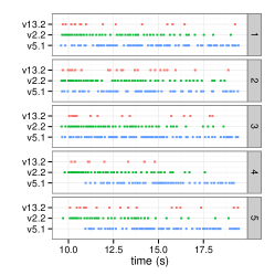
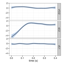
Figure 1: Left: Data example consisting of three spike tracks from five independent multichannel measurements of turtle spinal neurons during a stimulation period. Middel: Estimates of the $h_{i}$’s in the model of v2.2 using the direct approximation to minimize (9) with $n=20609$, $N=200$ and $q=33$. The value of $\lambda=0.016$ was chosen data adaptively. The baseline estimate is $\hat{\beta}_{0}=3.83$. Right: Similar estimates of the $h_{i}$’s using a B-spline basis expansion to minimize (11) with $q=33$, and with $\lambda=0.088$ chosen data adaptively. The baseline estimate is $\hat{\beta}_{0}=3.85$. The point-wise approximate 95% confidence intervals were obtained using a sandwich estimator of the asymptotic variance.

We have implemented both the direct approximation and the basis expansion using cubic B-spline basis functions and applied them to a test data set of neuron spike times. The data set consisted of multichannel measurements of spinal neurons from a turtle. The measurements were replicated 5 times and each time the spike activity was recorded over a period of 40 seconds. A 10 seconds stimulation was given within the observation window. We used the spike times for 3 neurons during the stimulation period, see Figure 1

The likelihood and gradient algorithms are implemented in the R package ppstat, which supports optimization of the objective function via the R function optim using the BFGS-algorithm. The ppstat package offers a formula based model specification with an interface familiar from glm. The direct approximation is implemented via the ppKernel function and the basis expansion is implemented via the ppSmooth function. A typical call has the form

ppKernel(v2.2 ~ k(v13.2) + k(v2.2) + k(v5.1),
                     data = spikeData,
                     family = Hawkes("logaffine"),
                     support = 0.2
)

which will include a baseline parameter in addition to the three non-parametric filter functions. The data set contained in the object spikeData must be of class MarkedPointProcess from the supporting R package processdata. The grid of $n$ time points is currently determined when the MarkedPointProcess object is constructed. The choice of $\varphi$ is specified by the “inverse link function” – being "logaffine" in the call above. This function will be used throughout, and it is given as

$$\varphi(x)=\left\{\begin{array}[]{ll}e^{x}&\quad\text{for }x\leq 0\\ x+1&\quad\text{for }x>0.\end{array}\right.$$

It maps $\mathbb{R}$ into $(0,\infty)$ and is continuously differentiable. The benefit of using this $\varphi$ over the exponential function is that the exponential function tends to produce models that are unstable or even explodes in finite time. We will not pursue the details. See Bremaud:1996 for details on stability.

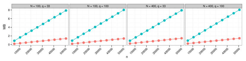
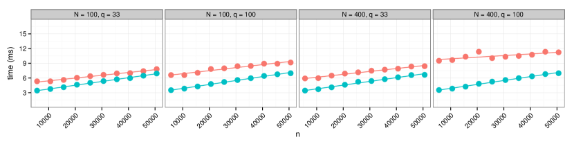
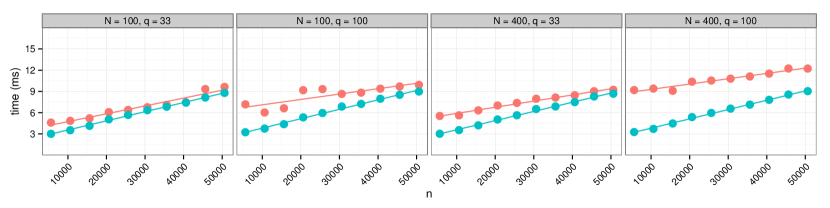
Figure 2: Top: Memory usage for storing the $\mathbf{H}$-matrix for the direct approximation ($\CIRCLE$) and the $\mathbf{Z}$-matrix for basis expansion ($\CIRCLE$) for $N=100,400$ and $q=33,100$. Middel: Log-likelihood computation time. Bottom: Gradient computation time.

Figure 1 shows the estimated $h_{i}$’s obtained using either the direct approximation with the Sobolev kernel or the basis expansion with a B-spline basis. The estimates were computed by minimizing (9) and (11), respectively. The Sobolev kernel is the reproducing kernel for the Sobolev Hilbert space consisting of twice weakly differentiable functions with the second derivative being square integrable. Its precise form depends on which inner product is chosen, but for common choices $R(\delta_{k},\cdot)$ is a cubic spline.

The choice of the penalization parameter was made data adaptively by minimizing a TIC-criterion, see Burnham:2002 . We will not pursue the details of the model selection procedure here, but focus on the efficiency of the computations of the likelihood and gradient. The resulting model shows that a v2.2 spike results in a depression of the v2.2-intensity in the first 0.1 seconds after the spike followed by an elevation of the v2.2-intensity. A v13.2 spike appears to result in a small but significant elevation of the v2.2-intensity, whereas a v5.1 spike appears to have no significant effect on the v2.2-intensity.

We investigated the memory usage and the computation times of both approximations. The memory usage was obtained using the R function object.size and the computation times were computed as the average of 40 replicated likelihood or gradient evaluations. The interest was on how they scale with the numbers $n$, $N$ and $q$ that determine the resolution of the time discretization and the dimension of the actual parameter space. For the basis expansion the number of B-spline basis functions was chosen explicitly to be either $q=33$ or $q=100$, and the choice of $N$ only affects the precomputation of the model matrices and not the likelihood and gradient computations. For the direct approximation the implementation uses the spectral decomposition, and $q$ is determined by a threshold on the size of the eigenvalues for $\mathbb{G}$ relative to the largest eigenvalue. The choice of threshold was tuned to result in $q=33$ or $q=100$. The implementation relies on precomputation of the $\mathbf{H}$ or $\mathbf{Z}$ matrices, which are stored as sparse matrices as implemented in the R package Matrix.

Figure 2 shows that basis expansion used more memory for storing $\mathbf{Z}$ and that the memory usage as a function of $n$ had a somewhat larger slope than for the direct approximation. We should note that the memory usage for neither of the methods showed a noticeable dependence upon $N$ or $q$. Storing the matrices as non-sparse matrices the $\mathbf{Z}$-matrix required 119 MB and the $\mathbf{H}$-matrix required 465 MB for $n=50000$, $N=400$ and $q=100$. In comparison, the sparse versions required 8 MB and 1.5 MB, respectively.

Figure 2 shows, furthermore, that likelihood and gradient computations were generally faster when the basis expansion was used. More importantly, Figure 2 shows that computation time for the direct approximation depended upon $N$ as well as $q$, and that the computation times for the basis expansion, using the B-spline basis, were remarkedly independent of $q$.

5 Discussion

The two approximations considered in this paper differ in terms of what is precomputed. Computing the matrix $\mathbf{H}$ upfront as in the direct approximation should require only a fraction of the memory required for storing the $\mathbf{Z}$-matrices. This was confirmed by our implementation. We also showed that the storage requirements for the direct approximation did not depend noticeably on the number $N$ of $\delta$-grid points when $\mathbf{H}$ is stored as a sparse matrix. The tradeoff is an increased computation time, which depends on the resolution determined by $N$ and $q$.

The storage requirements for $\mathbf{Z}$ can easily become prohibitively large. A choice of basis functions with local support, such as B-splines used here, can compensate partly for this. It is unlikely that it is useful to precompute $\mathbf{Z}^{i}V^{-1}$, as this will destroy the computational benefits of the basis with local support.

For the basis expansion it is possible to precompute the model matrix in a sligthly different and more direct way. Instead of precomputing the $q\times N$ basis function evaluations $B_{j}(\delta_{k})$ we can compute $\mathbf{Z}_{lj}^{i}$ directly as

$$\mathbf{Z}_{lj}^{i}=\sum_{k:t_{l}-A<\sigma_{k}^{i}<t_{i}}B_{j}(t_{l}-\sigma_{k}^{i}).$$

This may be more accurate but since $n\gg N$ in typical applications this comes at the cost of many more basis function evaluations. Whether this is critical in terms of the time to compute $\mathbf{Z}^{i}$ depends upon how costly a single basis function evaluation is relative to the computation of the $h_{lik}$’s. We have not presented data on the computational costs of the precomputations, but they were observed to be small compared to the costs of the actual optimization.

We observed that the fitted models obtained by either the direct approximation using the Sobolev kernel or the B-spline basis expansion were almost identical. This is not surprising given the fact that $R(\delta_{k},\cdot)$ is a cubic spline. In the actual implementation there are minor differences – for the B-spline expansion the linear part is, for instance, not penalized whereas all parts of the kernel fit is penalized. In conclusion, the B-spline basis expansion is currently to be preferred if the storage requirements can be met. The implementation of the direct approximation does, however, offer an easy way to use alternative kernels and thus alternative reproducing kernel Hilbert spaces.

We illustrated the general methods and the implemenation using neuron network data. Neuron network activity is just one example of a multivariate interacting dynamical system that is driven by discrete events. Other examples include high-frequency trading of multiple financial assets, see Hautsch:2004 , and chemical reaction networks as discussed in Anderson:2011 and Bowsher:2010 . The Markovian linear Hawkes model (1) was also considered in Chapter 7 in Hautsch:2004 , and the typical models of chemical reactions are Markovian multitype birth-death processes. Markovian models are often computationally advantageous, as they offer more efficient intensity and thus likelihood computations. With the implementation in the R package ppstat we have made more flexible yet computationally tractable non-parametric and non-Markovian models available.

6 Proof of Proposition 1

First note that since function evaluations are represented in terms of the kernel by inner products we have that

$$X_{s}(g) = \sum_{i=1}^{p}\sum_{j:\sigma_{j}^{i}<s}\langle R(s-\sigma_{j}^{i},\cdot),\ g_{i}\rangle$$ (12)

$$= \sum_{i=1}^{p}\left\langle\sum_{j:\sigma_{j}^{i}<s}R(s-\sigma_{j}^{i},\cdot),\ g_{i}\right\rangle.$$

If $\psi$ is a continuous differentiable function we find that

$$\frac{\psi(X_{s}(g+\varepsilon h))-\psi(X_{s}(g))}{\varepsilon}$$

$$\hskip 2.84526pt=\frac{\psi(X_{s}(g)+\varepsilon X_{s}(h))-\psi(X_{s}(g))}{\varepsilon}\longrightarrow\psi^{\prime}(X_{s}(g))X_{s}(h)$$

for $\varepsilon\rightarrow 0$. This is clearly a continuous linear functional. Using (12) and differentiating only w.r.t. the $i$’th coordinate of $g$ we find that the corresponding gradient in $\mathcal{H}$ is

$$\nabla_{i}\psi(X_{s}(g))=\psi^{\prime}(X_{s}(g))\sum_{j:\sigma_{j}^{i}<s}R(s-\sigma_{j}^{i},\cdot).$$

Taking $\psi=\log\varphi$ this yields the gradient of the second term in the negative log-likelihood, $\sum_{k=1}^{N_{t}}\log\varphi(X_{\tau_{k}}(g))$, directly. For the first term we take $\psi=\varphi$, but we need to ensure that we can interchange the order of integration and differentiation. To this end the following norm bound on $\nabla_{i}\varphi(X_{s}(g))$ is useful

$$||\nabla_{i}\varphi(X_{s}(g))|| \leq |\varphi^{\prime}(X_{s}(g))|\sum_{j:\sigma_{j}^{i}<s}||R(s-\sigma_{j}^{i},\cdot)||$$

$$\leq C_{t}N^{i}_{t}\sup_{s\in[0,t]}\sqrt{R(s,s)}<\infty.$$

Here $C_{t}=\sup_{s\in[0,t]}|\varphi^{\prime}(X_{s}(g))|$ is finite because $X_{s}(g)$ is continuous in $s$ and $\varphi^{\prime}$ is assumed continuous. We have also used that $||R(s-\sigma_{j}^{i},\cdot)||^{2}=R(s-\sigma_{j}^{i},s-\sigma_{j}^{i})$ and the fact that $R$ is continuous to conclude that the bound is finite. The bound shows that

$$\sum_{j}\int_{\sigma_{j}^{i}}^{t}\varphi^{\prime}(X_{s}(g))R(s-\sigma_{j}^{i},\cdot)\,\mathrm{d}s$$

is an element in $\mathcal{H}$ and the required interchange of integration and differentiation is justified by the bound. This completes the proof. ∎

- (1) Andersen, P.K., Borgan, Ø., Gill, R.D., Keiding, N.: Statistical models based on counting processes. Springer Series in Statistics. Springer-Verlag, New York (1993)
- (2) Anderson, D., Kurtz, T.: Continuous time markov chain models for chemical reaction networks. In: H. Koeppl, G. Setti, M. di Bernardo, D. Densmore (eds.) Design and Analysis of Biomolecular Circuits, pp. 3–42. Springer New York (2011). DOI 10.1007/978-1-4419-6766-4˙1. URL http://dx.doi.org/10.1007/978-1-4419-6766-4_1
- (3) Berlinet, A., Thomas-Agnan, C.: Reproducing kernel Hilbert spaces in probability and statistics. Kluwer Academic Publishers, Boston, MA (2004). With a preface by Persi Diaconis
- (4) Bishop, C.M.: Pattern Recognition and Machine Learning (Information Science and Statistics). Springer-Verlag New York, Inc., Secaucus, NJ, USA (2006)
- (5) Bowsher, C.G.: Stochastic kinetic models: Dynamic independence, modularity and graphs. Annals of Statistics 38(4), 2242–2281 (2010)
- (6) Brémaud, P., Massoulié, L.: Stability of nonlinear Hawkes processes. Ann. Probab. 24(3), 1563–1588 (1996)
- (7) Burnham, K.P., Anderson, D.R.: Model selection and multimodel inference, second edn. Springer-Verlag, New York (2002). A practical information-theoretic approach
- (8) Hansen, N.R.: Penalized maximum likelihood estimation for generalized linear point processes pp. 1–33 (2013). URL http://arxiv.org/abs/1003.0848
- (9) Hastie, T., Tibshirani, R., Friedman, J.: The elements of statistical learning, second edn. Springer Series in Statistics. Springer, New York (2009). DOI 10.1007/978-0-387-84858-7. URL http://dx.doi.org/10.1007/978-0-387-84858-7. Data mining, inference, and prediction
- (10) Hautsch, N.: Modelling irregularly spaced financial data, Lecture Notes in Economics and Mathematical Systems, vol. 539. Springer-Verlag, Berlin (2004). Theory and practice of dynamic duration models, Dissertation, University of Konstanz, Konstanz, 2003
- (11) Hawkes, A.G.: Spectra of some self-exciting and mutually exciting point processes. Biometrika 58(1), pp. 83–90 (1971). URL http://www.jstor.org/stable/2334319
- (12) Hofmann, T., Schölkopf, B., Smola, A.J.: Kernel methods in machine learning. Ann. Statist. 36(3), 1171–1220 (2008). DOI 10.1214/009053607000000677. URL http://dx.doi.org/10.1214/009053607000000677
- (13) Jacobsen, M.: Point process theory and applications. Probability and its Applications. Birkhäuser Boston Inc., Boston, MA (2006). Marked point and piecewise deterministic processes
- (14) Pillow, J.W., Shlens, J., Paninski, L., Sher, A., Litke, A.M., Chichilnisky, E.J., Simoncelli, E.P.: Spatio-temporal correlations and visual signalling in a complete neuronal population. Nature 454, 995–999 (2008)
- (15) Scholkopf, B., Smola, A.J.: Learning with Kernels: Support Vector Machines, Regularization, Optimization, and Beyond. MIT Press, Cambridge, MA, USA (2001)