A general theory for nonlinear sufficient dimension reduction: Formulation and estimation

Abstract

In this paper we introduce a general theory for nonlinear sufficient dimension reduction, and explore its ramifications and scope. This theory subsumes recent work employing reproducing kernel Hilbert spaces, and reveals many parallels between linear and nonlinear sufficient dimension reduction. Using these parallels we analyze the properties of existing methods and develop new ones. We begin by characterizing dimension reduction at the general level of $\sigma$-fields and proceed to that of classes of functions, leading to the notions of sufficient, complete and central dimension reduction classes. We show that, when it exists, the complete and sufficient class coincides with the central class, and can be unbiasedly and exhaustively estimated by a generalized sliced inverse regression estimator (GSIR). When completeness does not hold, this estimator captures only part of the central class. However, in these cases we show that a generalized sliced average variance estimator (GSAVE) can capture a larger portion of the class. Both estimators require no numerical optimization because they can be computed by spectral decomposition of linear operators. Finally, we compare our estimators with existing methods by simulation and on actual data sets.

, and

t1Supported in part by NSF Grants DMS-08-06058 and DMS-11-06815.

1 Introduction

In this paper we propose a general theory for nonlinear sufficient dimension reduction (SDR), develop novel estimators and investigate their properties under this theory. Along with these developments we also introduce a new conditional variance operator, which can potentially be used to generalize all second-order dimension reduction methods to the nonlinear case.

In its classical form, linear SDR seeks a low-dimensional linear predictor that captures in full a regression relationship. Imagining a regression setting that comprises multiple predictor variables and multiple responses, let $X$ and $Y$ be random vectors of dimension $p$ and $q$. If there is a matrix $\beta\in\mathbb{R}^{p\times d}$ with $d<p$ such that

$$Y\perp\perp X|\beta^{\mathsf{T}}X,$$ (1)

then the subspace spanned by the columns of $\beta$ is called a sufficient dimension reduction (SDR) subspace. Under mild conditions, the intersection of all such subspaces still satisfies (1), and is called the central subspace, denoted by ${\cal S}_{Y|X}$; see Li (1991, 1992), Li and Duan (1989), Duan and Li (1991), Cook and Weisberg (1991), Cook (1994, 1998b). A general condition for the existence of the central subspace is given by Yin, Li and Cook (2008).

Several recent papers have combined sufficient dimension reduction and kernels; see Akaho (2001), Bach and Jordan (2002), Fukumizu, Bach and Gretton (2007), Wu (2008), Wu, Liang and Mukherjee (2008), Hsing and Ren (2009), Yeh, Huang and Lee (2009), Zhu and Li (2011) and Li, Artemiou and Li (2011). This proliferation of work, in addition to producing versatile methods for extracting nonlinear sufficient predictors, points toward a general synthesis between the notions of sufficiency at the core of SDR and the ability to encompass nonlinearity afforded by kernel mappings. To achieve this synthesis, explore its many ramifications and broad scope and develop new estimators based on it, are the goals of this paper.

Specifically, we articulate a general formulation that comprises both linear and nonlinear SDR, and parallels the basic theoretical developments pioneered by Li (1991, 1992) and Cook (1994, 1998a, 1998b). This formulation allows us to study linear and nonlinear SDR comparatively and, somewhat surprisingly, to relax some stringent conditions required by linear SDR. For example, a linear conditional mean [Li (1991), Cook (1998b)] is no longer needed for unbiasedness, and the sufficient conditions for existence and uniqueness of the central subspace are far more general and transparent. Finally, our general formulation links linear and nonlinear SDR to the classical notions sufficiency, completeness and minimal sufficiency, which brings insights and great clarity to the SDR theory.

Our developments and the sections of this paper, can be summarized as follows. In Section 2, we build upon the ideas of Cook (2007) and Li, Artemiou and Li (2011) to define an SDR $\sigma$-field as a sub $\sigma$-field ${\cal G}$ of $\sigma(X)$ (the $\sigma$-field generated by $X$) such that $Y\perp\perp X|{\cal G},$ and the corresponding SDR class as the set of all square-integrable, ${\cal G}$-measurable functions. Under very mild conditions—much milder than the corresponding conditions for linear SDR [Yin, Li and Cook (2008)]—we show that there exists a unique minimal $\sigma$-field ${{\cal G}_{Y|X}}$ that satisfies $Y\perp\perp X|{{\cal G}_{Y|X}}$, which we call the central $\sigma$-field. The set of all ${{\cal G}_{Y|X}}$-measurable, square-integrable functions is named the central class.

In Section 3, we provide two additional definitions that generalize concepts in Cook (1998b), Li, Zha and Chiaromonte (2005) and Li, Artemiou and Li (2011): a class of functions is unbiased if its members are ${{\cal G}_{Y|X}}$-measurable, and exhaustive if they generate ${{\cal G}_{Y|X}}$. Next, we show that the special class

$${L_{2}(P_{X})}\ominus\bigl{[}{L_{2}(P_{X})}\ominus{L_{2}(P_{Y})}\bigr{]}$$ (2)

is unbiased, where ${L_{2}(P_{X})}$ and ${L_{2}(P_{Y})}$ are the spaces of square-integrable functions of $X$ and $Y$. For reasons detailed in Section 3, we call this class the regression class.

In Section 4, we introduce the complete dimension reduction class: if ${\cal G}\subseteq\sigma(X)$ is a $\sigma$-field and for each ${\cal G}$-measurable $f\in{L_{2}(P_{X})}$ we have

$$E\bigl{(}f(X)|Y\bigr{)}=0\qquad\mbox{almost surely}\quad\Rightarrow\quad f(X)=0\qquad\mbox{almost surely},$$

then we say that the class of ${\cal G}$-measurable functions in ${L_{2}(P_{X})}$ is complete. We prove that when a complete sufficient dimension reduction (CSDR) class exists it is unique and coincides with the central class. We further show that the CSDR class coincides with the regression class—which is therefore not just unbiased, but also exhaustive.

In Section 5 we establish a critical relationship between the regression class and a covariance operator linking $X$ and $Y$ and, based on this, we generalize sliced inverse regression [SIR; Li (1991)] to a method (GSIR) that can recover the regression class—and hence is unbiased and exhaustive under completeness. In Section 6, we consider the case where the central class is not complete, so that GSIR is unbiased but no longer exhaustive. By introducing a novel conditional variance operator, we generalize sliced average variance estimation [SAVE, Cook and Weisberg (1991)] to a method (GSAVE) that can recover a class larger than the regression class. Here, the situation is similar to that in the linear SDR setting, where it is well known that

$$\mbox{SIR subspace}\subseteq\mbox{SAVE subspace}\subseteq{\cal S}_{Y|X};$$ (3)

see Cook and Critchley (2000), Ye and Weiss (2003), Li, Zha and Chiaromonte (2005) and Li and Wang (2007).

In Section 7 we develop algorithms for the sample versions of GSIR and GSAVE, and a cross-validation algorithm to determine regularizing parameters. In Section 8 we compare GSIR and GSAVE with some existing methods by simulation and on actual data sets. Section 9 contains some concluding remarks. Some highly technical developments are provided in the supplementary material [Lee, Li and Chiaromonte (2013)].

2 Sufficient dimension reduction $\sigma$-fields and classes

Let $(\Omega,{\cal F},P)$ be a probability space and $(\Omega_{X},{\cal F}_{X})$, $(\Omega_{Y},{\cal F}_{Y})$ and $(\Omega_{XY},{\cal F}_{XY})$ be measurable spaces. For convenience, assume that $\Omega_{XY}=\Omega_{X}\times\Omega_{Y}$ and ${\cal F}_{XY}={\cal F}_{X}\times{\cal F}_{Y}$. Let $X$, $Y$ and $(X,Y)$ be random elements that take values in $\Omega_{X}$, $\Omega_{Y}$ and $\Omega_{XY}$, with distributions $P_{X}$, $P_{Y}$, $P_{XY}$, which are dominated by $\sigma$-finite measures. Let

$$\sigma(X)=X^{-1}({\cal F}_{X}),\qquad\sigma(Y)=Y^{-1}({\cal F}_{Y}),\qquad\sigma(X,Y)=(X,Y)^{-1}({\cal F}_{XY}),$$

and finally let $P_{Y|X}(\cdot|\cdot)\dvtx{\cal F}_{Y}\times\Omega_{X}\to{\cal R}$ be the conditional distribution of $Y$ given $X$.

Definition 1.

A sub $\sigma$-field ${\cal G}$ of $\sigma(X)$ is an SDR $\sigma$-field for $Y$ versus $X$ if it satisfies

$$Y\perp\perp X|{\cal G},$$ (4)

that is, if $Y$ and $X$ are independent given ${\cal G}$.

This definition is sufficiently general to accommodate the two cases of nonlinear sufficient dimension reduction that interest us the most. The first case is when $\Omega_{X}=\mathbb{R}^{p}$ and $\Omega_{Y}=\mathbb{R}^{q}$ for some positive integers $p$ and $q$, and ${\cal F}_{X}$, ${\cal F}_{Y}$ and ${\cal F}_{XY}$ are Borel $\sigma$-fields generated by the open sets in $\mathbb{R}^{p}$, $\mathbb{R}^{q}$ and $\mathbb{R}^{p+q}$. Clearly, in this case, the conditional independence (4) is a generalization of (1) for linear SDR: if we take ${\cal G}=\sigma(\beta^{\mathsf{T}}X)$, then (4) reduces to (1).

The second case is when $X$ or $Y$, or both of them, are random functions. In this case Definition 1 is a generalization of the linear SDR for functional data introduced by Ferré and Yao (2003), and Hsing and Ren (2009). Specifically, let $[a,b]$ be a closed interval, $\lambda$ the Lebesgue measure and $L_{2}(\lambda)$ the class of functions on $[a,b]$ that are square integrable with respect to $\lambda$. Let $\Omega_{X}=L_{2}(\lambda)$ and $\Omega_{Y}=\mathbb{R}$. In this case, each $X(\omega)$ is a function in $L_{2}(\lambda)$, which, depending on applications, could be, say, a growth curve or the fluctuation of a stock price. Let $h_{1},\ldots,h_{d}$ be functions in $L_{2}(\lambda)$. Ferré and Yao (2003) considered the following functional dimension reduction problem:

$$Y\perp\perp X|\langle X,h_{1}\rangle_{L_{2}(\lambda)},\ldots,\langle X,h_{d}\rangle_{L_{2}(\lambda)}.$$ (5)

This generalizes linear SDR to the infinite-dimensional case, but not to the nonlinear case, because $\langle X,h_{1}\rangle_{L_{2}(\lambda)},\ldots,\langle X,h_{d}\rangle_{L_{2}(\lambda)}$ are linear in $X$. Hsing and Ren (2009) considered a more general setting where the sample paths $\{X_{t}(\omega)\dvtx t\in J\}$ need not lie within $L_{2}(\lambda)$. Still, their generalization is inherently linear in the same sense that problem (5) is linear. In contrast, our formulation in (4) allows an arbitrary sub $\sigma$-field of $\sigma(X)$, which need not be generated by linear functionals. Interestingly, as we will see Section 5, it is the relaxation of linearity that allows us to remove a restrictive linear conditional mean assumption used both in Ferré and Yao (2003) (Theorem 2.1), and in Hsing and Ren (2009), assumption (IR2).

The notion of sufficiency underlying SDR, as defined by (1) and (4), is different from the classical notion of sufficiency because $\cal G$ is allowed to depend on any parameter in the joint distribution of $P_{XY}$. For example, ${\cal G}=\sigma(\beta^{\mathsf{T}}X)$ depends on the parameter $\beta$ [or rather, the meta-parameter $\operatorname{span}(\beta)$] which characterizes the conditional distribution of $Y|X$. Nevertheless, both notions imply a reduction, or simplification, in the representation of a stochastic mechanism—the SDR one through a newly constructed predictor, and the classical one through a statistic. Indeed, it is partly by exploring and exploiting this similarity that we developed our theory of nonlinear SDR.

Obviously there are many sub $\sigma$-fields of $X$ that satisfy (4), starting with $\sigma(X)$ itself—which induces no reduction. For maximal dimension reduction we seek the smallest such $\sigma$-field. As in the case of classical sufficiency, the minimal $\mathrm{SDR}$ $\sigma$-field does not universally exist, but exists under very mild assumptions. The next theorem gives the sufficient condition for the minimal $\mathrm{SDR}$ $\sigma$-field to uniquely exist. The proof echoes Bahadur (1954), which established the existence of the minimal sufficient $\sigma$-field in the classical setting.

Theorem 1.

Suppose that the family of probability measures $\{P_{X|Y}(\cdot|y)\dvtx\break y\in\Omega_{Y}\}$ is dominated by a $\sigma$-finite measure. Then there is a unique sub $\sigma$-field ${\cal G}^{*}$ of $\sigma(X)$ such that: [(2)]

$Y\perp\perp X|{\cal G}^{*}$;

if ${\cal G}$ is a sub $\sigma$-field of $\sigma(X)$ such that $Y\perp\perp X|{\cal G}$, then ${\cal G}^{*}\subseteq{\cal G}$.

Let $\Pi_{y}=P_{X|Y}(\cdot|y)$ and $\mathbb{P}=\{\Pi_{y}\dvtx y\in\Omega_{Y}\}$. Since $\mathbb{P}$ is dominated by a $\sigma$-finite measure, it contains a countable subset $\mathbb{Q}=\{Q_{k}\dvtx k=1,2,\ldots\}$ such that $\mathbb{Q}\equiv\mathbb{P}$, where $\equiv$ means two families of measures dominating each other. Let $\{c_{k}\dvtx k=1,2,\ldots\}$ be a sequence of positive numbers that sum to 1, and let $Q_{0}=\sum_{k=1}^{\infty}c_{k}Q_{k}$. Then $Q_{0}$ is a probability measure on $\Omega_{X}$ such that $\{Q_{0}\}\equiv\mathbb{Q}\equiv\mathbb{P}$. Let $\pi_{y}=d\Pi_{y}/dQ_{0}$ and ${\cal G}$ be a sub $\sigma$-field of $\sigma(X)$. We claim that the following statements are equivalent: [(2)]

$Y\perp\perp X|{\cal G}$;

$\pi_{y}$ is essentially measurable with respect to ${\cal G}$ for all $y\in\Omega_{Y}$ modulo $Q_{0}$.

Proof of 1 $\Rightarrow$ 2. Let $B\in{\cal F}_{X}$. Then

$$E_{Q_{0}}\bigl{(}\pi_{y}(X)I_{B}(X)\bigr{)} = E_{\Pi_{y}}\bigl{(}I_{B}(X)\bigr{)}=E_{\Pi_{y}}\bigl{[}E_{\Pi_{y}}\bigl{(}I_{B}(X)|{\cal G}\bigr{)}\bigr{]}$$

$$= E_{Q_{0}}\bigl{[}E_{\Pi_{y}}\bigl{(}I_{B}(X)|{\cal G}\bigr{)}\pi_{y}(X)\bigr{]}.$$

By 1, $\Pi_{y}(B|{\cal G})$ is the same for all $y\in\Omega_{Y}$. Hence $\Pi_{y}(B|{\cal G})=Q_{k}(B|{\cal G})$ for all $k$, which implies $\Pi_{y}(B|{\cal G})=Q_{0}(B|{\cal G})$. Hence we can rewrite the right-hand side of the above equalities as

$$E_{Q_{0}}\bigl{[}E_{Q_{0}}\bigl{(}I_{B}(X)|{\cal G}\bigr{)}\pi_{y}(X)\bigr{]}=E_{Q_{0}}\bigl{[}I_{B}(X)E_{Q_{0}}\bigl{(}\pi_{y}(X)|{\cal G}\bigr{)}\bigr{]}.$$

Thus the following equality holds for all $B\in{\cal F}_{X}$:

$$E_{Q_{0}}\bigl{(}\pi_{y}(X)I_{B}(X)\bigr{)}=E_{Q_{0}}\bigl{[}I_{B}(X)E_{Q_{0}}\bigl{(}\pi_{y}(X)|{\cal G}\bigr{)}\bigr{]},$$

which implies $\pi_{y}(X)=E_{Q_{0}}(\pi_{y}(X)|{\cal G})$ a.s. $Q_{0}$.

Proof of 2 $\Rightarrow$ 1. For any $A\in{\cal G}$,

$$E_{\Pi_{y}}\bigl{[}E_{Q_{0}}\bigl{(}I_{B}(X)|{\cal G}\bigr{)}I_{A}(X)\bigr{]} = E_{Q_{0}}\bigl{[}E_{Q_{0}}\bigl{(}I_{B}(X)|{\cal G}\bigr{)}I_{A}(X)\pi_{y}(X)\bigr{]}$$

$$= E_{Q_{0}}\bigl{[}I_{B}(X)I_{A}(X)E_{Q_{0}}\bigl{(}\pi_{y}(X)|{\cal G}\bigr{)}\bigr{]}.$$

By 2, $E_{Q_{0}}(\pi_{y}(X)|{\cal G})=\pi_{y}(X)$. Hence the right-hand side becomes

$$E_{Q_{0}}\bigl{[}I_{B}(X)I_{A}(X)\pi_{y}(X)\bigr{]}=E_{\Pi_{y}}\bigl{[}I_{B}(X)I_{A}(X)\bigr{]}=\Pi_{y}(X\in A\cap B).$$

Thus $E_{Q_{0}}(I_{B}(X)|{\cal G})=Q_{0}(B|{\cal G})$ is the conditional probability $\Pi_{y}(B|{\cal G})$, which means $\Pi_{y}(B|{\cal G})$ does not depend on $y$. That is, 1 holds.

Now let ${\cal G}^{*}$ be the intersection of all $\mathrm{SDR}$ $\sigma$-fields ${\cal G}$. Then ${\cal G}^{*}$ is itself a $\sigma$-field. Moreover, since $\pi_{y}$ is essentially measurable with respect to all $\mathrm{SDR}$ $\sigma$-fields for all $y\in\Omega_{Y}$, it is also essentially measurable with respect to ${\cal G}^{*}$ for all $y\in\Omega_{Y}$. Consequently, ${\cal G}^{*}$ is itself an $\mathrm{SDR}$ $\sigma$-field, which implies that it is also the smallest $\mathrm{SDR}$ $\sigma$-field. If ${\cal G}^{**}$ is another smallest $\mathrm{SDR}$ $\sigma$-field, then we know ${\cal G}^{*}\subseteq{\cal G}^{**}$ and ${\cal G}^{**}\subseteq{\cal G}^{*}$. Thus ${\cal G}^{*}$ is unique.

We can now naturally introduce the following definition:

Definition 2.

Suppose that the class of probability measures $\{P_{X|Y}(\cdot|y)\dvtx\break y\in\Omega_{Y}\}$ on $\Omega_{X}$ is dominated by a $\sigma$-finite measure. Then we call the $\sigma$-field ${\cal G}^{*}$ in Theorem 1 the central $\sigma$-field for $Y$ versus $X$, and denote it by ${\cal G}_{Y|X}$.

Notably, this set up characterizes dimension reduction solely in terms of conditional independence. However, explicitly turning to functions and introducing an additional mild assumption of square integrability are very consequential for further development because they allow us to work with structures such as orthogonality and projection.

Let $L_{2}(P_{XY})$, $L_{2}(P_{X})$ and $L_{2}(P_{Y})$ be the spaces of functions defined on $\Omega_{XY}$, $\Omega_{X}$ and $\Omega_{Y}$ that are square-integrable with respect to $P_{XY}$, $P_{X}$ and $P_{Y}$, respectively. Since constants are irrelevant for dimension reduction, we assume throughout that all functions in ${L_{2}(P_{X})}$, ${L_{2}(P_{Y})}$ and $L_{2}(P_{XY})$ have mean 0. Given a sub $\sigma$-field ${\cal G}$ of $\sigma(X,Y)$, we use $\mathfrak{M}_{\cal G}$ to denote the class of all functions $f$ in $L_{2}(P_{XY})$ such that $f(X)$ is ${\cal G}$-measurable. If ${\cal G}$ is generated by a random vector, say $X$, then we use $\mathfrak{M}_{X}$ to abbreviate $\mathfrak{M}_{\sigma{(X)}}$. It can be easily shown that, for any ${\cal G}$, $\mathfrak{M}_{\cal G}$ is a linear subspace of $L_{2}(P_{XY})$.

Definition 3.

Let ${\cal G}$ be an $\mathrm{SDR}$ $\sigma$-field and ${\cal G}_{Y|X}$ be the central $\sigma$-field. Then $\mathfrak{M}_{\cal G}$ is called an $\mathrm{SDR}$ class, and $\mathfrak{M}_{{\cal G}_{Y|X}}$ is called the central class. The latter class is denoted by ${\mathfrak{S}}_{Y|X}$.

The central class, comprising square-integrable functions that are measurable with respect to the central $\sigma$-field ${\cal G}_{Y|X}$, represents our generalization of the central space ${\cal S}_{Y|X}$ defined in linear SDR; see the Introduction.

3 Unbiasedness and exhaustiveness

In linear SDR, the goal is to find a set of vectors that span ${\cal S}_{Y|X}$. If a matrix $\gamma$ satisfies $\operatorname{span}(\gamma)\subseteq{\cal S}_{Y|X}$, we say that $\gamma$ is unbiased [Cook (1998b)]. If $\operatorname{span}(\gamma)={\cal S}_{Y|X}$, we say that $\gamma$ is exhaustive [Li, Zha and Chiaromonte (2005)]. Note that when $\operatorname{span}(\gamma)\subseteq{\cal S}_{Y|X}$, $\gamma^{\mathsf{T}}X$ is a linear function of $\beta^{\mathsf{T}}X$, where $\beta$ is any matrix such that $\operatorname{span}(\beta)={\cal S}_{Y|X}$; if $\operatorname{span}(\gamma)={\cal S}_{Y|X}$, then $\gamma^{\mathsf{T}}X$ is an injective linear transformation of $\beta^{\mathsf{T}}X$. In the nonlinear setting, we follow the same logic but remove the linear requirement. Part of the following definition was given in Li, Artemiou and Li (2011).

Definition 4.

A class of functions in ${L_{2}(P_{X})}$ is unbiased for ${\mathfrak{S}}_{Y|X}$ if its members are ${{\cal G}_{Y|X}}$-measurable, and exhaustive for ${\mathfrak{S}}_{Y|X}$ if its members generate ${{\cal G}_{Y|X}}$.

Next, we look into what type of functions are unbiased. The lemma below provides a characterization of the orthogonal complement of $\mathfrak{M}_{{\cal G}}$ that will be used many times in the subsequent development. Its proof is essentially the definition of the conditional expectation, and is omitted.

Lemma 1

Suppose $U$ is a random element defined on $(\Omega,{\cal F})$, ${\cal G}$ is a sub $\sigma$-field of $\sigma(U)$ and $f\in L_{2}(P_{U})$. Then $f$ is orthogonal to $\mathfrak{M}_{\cal G}$ ($f\perp\mathfrak{M}_{\cal G}$) if and only if $E[f(U)|{\cal G}]=0$.

Note that $\perp\perp$ and $\perp$ have different meanings: the former means independence; the latter means orthogonality. For two subspaces, say ${\cal S}_{1}$ and ${\cal S}_{2}$, of a generic Hilbert space $\cal H$, we use ${\cal S}_{1}\ominus{\cal S}_{2}$ to denote the subspace ${\cal S}_{1}\cap{\cal S}_{2}^{\perp}$. The following theorem explicitly specifies a class of functions, which we call regression class, that is unbiased for ${\mathfrak{S}}_{Y|X}$.

Theorem 2.

If the family $\{\Pi_{y}\dvtx y\in\Omega_{Y}\}$ is dominated by a $\sigma$-finite measure, then

$$L_{2}(P_{X})\ominus\bigl{[}L_{2}(P_{X})\ominus L_{2}(P_{Y})\bigr{]}\subseteq{\mathfrak{S}}_{Y|X}.$$ (6)

It is equivalent to show that $L_{2}(P_{X})\ominus{\mathfrak{S}}_{Y|X}\subseteq L_{2}(P_{X})\ominus L_{2}(P_{Y}).$ If $f\in L_{2}(P_{X})\ominus{\mathfrak{S}}_{Y|X}$, then, by Lemma 1, $E[f(X)|{{\cal G}_{Y|X}}]=0$. Since ${{\cal G}_{Y|X}}$ is a sufficient $\sigma$-field,

$$E\bigl{[}f(X)|Y\bigr{]}=E\bigl{[}E\bigl{(}f(X)|Y,{{\cal G}_{Y|X}}\bigr{)}|Y\bigr{]}=E\bigl{[}E\bigl{(}f(X)|{{\cal G}_{Y|X}}\bigr{)}|Y\bigr{]}=0.$$

By Lemma 1 again, $f\perp\mathfrak{M}_{Y}$. Because $\mathfrak{M}_{Y}=L_{2}(P_{Y})$, we have $f\in L_{2}(P_{X})\ominus L_{2}(P_{Y})$.

The intuition behind the term “regression class” is that ${L_{2}(P_{X})}\ominus{L_{2}(P_{Y})}$ resembles the residual in a regression problem; thus ${L_{2}(P_{X})}\ominus[{L_{2}(P_{X})}\ominus{L_{2}(P_{Y})}]$ is simply the orthogonal complement of the “residual class.” Henceforth we write the regression class as ${\mathfrak{C}_{Y|X}}$.

4 Complete and sufficient dimension reduction classes

After showing that the regression class (2) is unbiased, we investigate under what conditions it is also exhaustive for the central class ${\mathfrak{S}}_{Y|X}$. To this end we need to introduce the notion of complete classes of functions in ${L_{2}(P_{X})}$.

Definition 5.

Let ${\cal G}\subseteq\sigma(X)$ be a sub $\sigma$-field. The class $\mathfrak{M}_{\cal G}$ is said to be complete if, for any $g\in\mathfrak{M}_{\cal G}$,

$$E\bigl{[}g(X)|Y\bigr{]}=0\qquad\mbox{a.s. }P\quad\Rightarrow\quad g(X)=0\qquad\mbox{a.s. }P.$$

Again there are similarities and differences between completeness as defined here and in the classical setting. A complete and sufficient statistic in the classical setting is a rather restrictive concept, often associated with exponential families, the uniform distribution, or the order statistics. In contrast, completeness here is a rather general concept. To demonstrate this point, in the next two propositions we give two examples of complete and sufficient dimension reduction classes. In particular, the first shows that if $Y$ is related to $X$ through any regression model with additive error, then the subspace of $L_{2}(P_{X})$ determined by the regression function is a complete and sufficient dimension reduction class. In the following, $[{L_{2}(P_{X})}]^{q}$ denotes the $q$-fold Cartesian product of ${L_{2}(P_{X})}$.

Proposition 1

Suppose there exists a function $h\in[{L_{2}(P_{X})}]^{q}$ such that

$$Y=h(X)+\varepsilon,$$ (7)

where $\varepsilon\perp\perp X$ and $E(\varepsilon)=0$. Then $\mathfrak{M}_{h(X)}$ is a complete and sufficient dimension reduction class for $Y$ versus $X$.

Note that, since ${L_{2}(P_{X})}$ is centered, we have implicitly assumed that $E[h(X)]=0$ [and hence $E(Y)=0$]. However, this does not entail any real loss of generality because the proof below can be easily modified for the case where ${L_{2}(P_{X})}$ is not centered.

Proof of Proposition 1 Suppose $m\in\mathfrak{M}_{h(X)}$ and $E[m(X)|Y]=0$ a.s. $P$. Then there is a measurable function $g\dvtx\mathbb{R}^{q}\to\mathbb{R}$ such that $m=g\circ h$. Let $U=h(X)$. Then $E(g(U)|Y)=0$ a.s. $P$. By Lemma 1, for any $f\in L_{2}(P_{Y})$, we have $E[g(U)f(Y)]=0$. In particular, $E[g(U)e^{it^{\mathsf{T}}Y}]=0.$ Because $U\perp\perp\varepsilon$, this implies

$$E\bigl{[}g(U)e^{it^{\mathsf{T}}U}\bigr{]}E\bigl{(}e^{it^{\mathsf{T}}\varepsilon}\bigr{)}=E\bigl{[}g(U)e^{it^{\mathsf{T}}U}e^{it^{\mathsf{T}}\varepsilon}\bigr{]}=E\bigl{[}g(U)e^{it^{\mathsf{T}}Y}\bigr{]}=0.$$

Hence $E[g(U)e^{it^{\mathsf{T}}U}]=0$. By the uniqueness of inverse Fourier transformation we see that $g(U)=0$ a.s. $P$, which implies $m(X)=(g\circ h)(X)=0$ a.s. $P$.

The expression in (7) covers many useful models in statistics and econometrics. For example, any homoscedastic parametric or nonparametric regression, such as the single index and the multiple index models [Ichimura and Lee (1991), Härdle, Hall and Ichimura (1993), Yin, Li and Cook (2008)], are special cases of (7). Thus, complete and sufficient dimension reduction classes exist for all those settings. The next proposition considers a type of inverse regression model, in which $X$ is transformed into two components, one of which is related to $Y$ by an inverse linear regression model, and the other independent of the rest of the data.

Proposition 2

Suppose $q<p$, $\Omega_{Y}$ has a nonempty interior, and $P_{Y}$ is dominated by the Lebesgue measure on $\mathbb{R}^{q}$. Suppose there exist functions $g\in[{L_{2}(P_{X})}]^{q}$ and $h\in[{L_{2}(P_{X})}]^{p-q}$ such that: [(4)]

$g(X)=Y+\varepsilon$, where $Y\perp\perp\varepsilon$, and $\varepsilon\sim N(0,\Sigma)$;

$\sigma(g(X),h(X))=\sigma(X)$;

$h(X)\perp\perp(Y,g(X))$;

the induced measure $P_{X}\circ g^{-1}$ is dominated by the Lebesgue measure on $\mathbb{R}^{q}$. Then $\mathfrak{M}_{g(X)}$ is a complete sufficient dimension reduction class for $Y$ versus $X$.

Assumption 3 implies $Y\perp\perp h(X)|g(X)$, which, by assumption 2, implies $Y\perp\perp X|g(X)$. That is, $\mathfrak{M}_{g(X)}$ is an SDR class. Let $u\in\mathfrak{M}_{g(X)}$. Then $u=v\circ g$ for some measurable function $v\dvtx\mathbb{R}^{q}\to\mathbb{R}$. Let $U=g(X)$. Suppose that $E[v(U)|Y]=0$ almost surely $P$. Because $Y\perp\perp\varepsilon$, this implies $P_{Y}(\{y\dvtx Ev(y+\varepsilon)=0\})=1$. In other words,

$$\int_{\mathbb{R}^{q}}v(t)\frac{1}{(2\pi)^{q/2}|\Sigma|^{1/2}}e^{-(t-y)^{\mathsf{T}}\Sigma^{-1}(t-y)/2}\,dt=0$$

a.s. $P_{Y}$. This implies

$$\int v(t)e^{-t^{\mathsf{T}}\Sigma^{-1}t/2}e^{y^{\mathsf{T}}\Sigma^{-1}t}\,dt=0\quad\Rightarrow\quad\int v(\Sigma s)e^{-s^{\mathsf{T}}\Sigma s/2}e^{y^{\mathsf{T}}s}\,ds=0$$

a.s. $P_{Y}$, where $s=\Sigma^{-1}t$. Because $\Omega_{Y}$ contains an open set in $\mathbb{R}^{q}$ and the above function of $y$ is analytic, by the analytic continuation theorem, the above function is 0 everywhere on $\mathbb{R}^{q}$. Hence, by the uniqueness of inverse Laplace transformation, we have

$$v(\Sigma s)e^{-s^{\mathsf{T}}\Sigma s/2}=0\qquad\mbox{almost surely $\lambda$},$$

where $\lambda$ is the Lebesgue measure on $\mathbb{R}^{q}$. But, because $e^{-s^{\mathsf{T}}\Sigma s/2}>0$, we have $v(\Sigma s)=0$ a.s. $\lambda$ or equivalently $v(t)=0$ a.s. $\lambda$. By the change of variable theorem,

$$\int_{v\circ g(x)\neq 0}dP_{X}=\int_{v(t)\neq 0}dP_{X}\circ g^{-1}.$$

By assumption 4, $P_{X}\circ g^{-1}\ll\lambda$. Hence the above integral is 0, implying $v\circ g(x)=0$ a.s. $P_{X}$, or, equivalently, $v\circ g(X)=0$ a.s. $P$.

Inverse regressions of this type are considered in Cook (2007), Cook and Forzani (2009), and Cook, Li and Chiaromonte (2010) for linear SDR. The above two propositions show that a complete and sufficient dimension reduction class exists for a reasonably wide range of problems, including forward and inverse regressions of very general, nonparameterized form. The next theorem shows that when a complete and sufficient dimension reduction class exists, it is unique and coincides with the central class. Once again, the situation here echoes that in classical theory, where a complete and sufficient statistic, if it exists, coincides with the minimal sufficient statistic; see Lehmann (1981).

Theorem 3.

Suppose $\{\Pi_{y}\dvtx y\in\Omega_{Y}\}$ is dominated by a $\sigma$-finite measure, and ${\cal G}$ is a sub $\sigma$-field of $\sigma(X)$. If $\mathfrak{M}_{\cal G}$ is a complete and sufficient dimension reduction class, then

$$\mathfrak{M}_{\cal G}={\mathfrak{C}_{Y|X}}={\mathfrak{S}}_{Y|X}.$$

If $f\perp{\mathfrak{C}_{Y|X}}$, then by Lemma 1, $E(f|Y)=0$ which, because $\mathfrak{M}_{\cal G}$ is sufficient, implies

$$E\bigl{[}E(f|{\cal G})|Y\bigr{]}=0.$$

Because $\mathfrak{M}_{\cal G}$ is complete and because $E(f|{\cal G})\in\mathfrak{M}_{\cal G}$, we have $E(f|{\cal G})=0$. By Lemma 1, this implies $f\perp\mathfrak{M}_{\cal G}$. Thus we have proved $\mathfrak{M}_{\cal G}\subseteq{\mathfrak{C}_{Y|X}}$. However, by Theorem 2 we know that ${\mathfrak{C}_{Y|X}}\subseteq{\mathfrak{S}}_{Y|X}\subseteq\mathfrak{M}_{\cal G}$. This proves the desired equality.

5 Generalizations of SIR and their population-level properties

From the previous developments we see that the subspace $L_{2}(P_{X})\ominus L_{2}(P_{Y})$ of $L_{2}(P_{X})$ plays a critical role in nonlinear SDR. Its orthogonal complement in $L_{2}(P_{X})$ coincides with the central class ${\mathfrak{S}}_{Y|X}$ under completeness, and even without completeness it is guaranteed to be inside ${\mathfrak{S}}_{Y|X}$. It turns out that this subspace can be expressed as the range of a certain bounded linear operators. This representation ensures that estimation procedures can rely on simple spectral decompositions, rather than complicated numerical optimizations. We first introduce some covariance operators which are the building block of this approach.

5.1 Covariance operators

Since constants are irrelevant here (e.g., $f$ and $f+3$ can be considered as the same function), we will speak of set relations modulo constants. If $A$ and $B$ are sets, then we say $A\subseteq B$ modulo constants if for each $f\in A$ there is $c\in\mathbb{R}$ such that $f+c\in B$. We say that $A$ is a dense subset of $B$ modulo constants if (i) $A\subseteq B$ modulo constants and (ii) for each $f\in B$, there is a sequence $\{f_{n}\}\subseteq A$ and a sequence of constants $\{c_{n}\}\subseteq\mathbb{R}$ such that $\{f_{n}+c_{n}\}\subseteq A$ and $f_{n}+c_{n}\to f$ in the topology for $B$. Let ${{\cal{H}}_{X}}$ and ${{\cal{H}}_{Y}}$ be Hilbert spaces of functions of $X$ and $Y$ satisfying the conditions: [(B)]

${{\cal H}_{X}}$ and ${{\cal H}_{Y}}$ are dense subsets of ${L_{2}(P_{X})}$ and ${L_{2}(P_{Y})}$ modulo constants;

there are constants $C_{1}>0$ and $C_{2}>0$ such that $\operatorname{var}[f(X)]\leq C_{1}\|f\|_{{\cal{H}}_{X}}$ and $\operatorname{var}[g(Y)]\leq C_{2}\|g\|_{{\cal{H}}_{Y}}$. Although we will later take ${{\cal{H}}_{X}}$ and ${{\cal{H}}_{Y}}$ to be reproducing kernel Hilbert spaces (RKHS), our theory is not restricted to such spaces. In particular, we do not require the evaluation functionals [such as $f\mapsto f(x)$ from ${{\cal{H}}_{X}}$ to $\mathbb{R}$] to be continuous.

For two generic Hilbert spaces ${\cal H}_{1}$ and ${\cal H}_{2}$, let ${\cal B}({\cal H}_{1},{\cal H}_{2})$ denote the class of all bounded linear operators from ${\cal H}_{1}$ to ${\cal H}_{2}$, and let ${\cal B}({\cal H}_{1})$ abbreviate ${\cal B}({\cal H}_{1},{\cal H}_{1})$. We denote the range of a linear operator $A$ by $\operatorname{ran}A$, the kernel of $A$ by $\ker A$, and the closure of $\operatorname{ran}A$ by $\operatorname{\overline{ran}}A$. Under assumption (B), the symmetric bilinear form $u\dvtx{{\cal{H}}_{X}}\times{{\cal{H}}_{X}}\to\mathbb{R}$ defined by $u(f,g)=\operatorname{cov}[f(X),g(X)]$ is bounded and thus induces an operator ${M_{XX}}\in{\cal B}({{\cal{H}}_{X}})$ that satisfies $\langle f,{M_{XX}}g\rangle_{{\cal{H}}_{X}}=u(f,g).$ Similarly, the bounded bilinear form $(f,g)\mapsto\operatorname{cov}[f(Y),g(Y)]$ from ${{\cal{H}}_{Y}}\times{{\cal{H}}_{Y}}$ to $\mathbb{R}$ defines an operator ${M_{YY}}\in{\cal B}({{\cal{H}}_{Y}})$. Let ${\cal G}_{X}$ and ${{\cal G}_{Y}}$ represent the subspaces $\operatorname{\overline{ran}}{M_{XX}}$ and $\operatorname{\overline{ran}}{M_{YY}}$.

Definition 6.

Suppose conditions (A) and (B) are satisfied. We define the covariance operators $\Sigma_{XX}\dvtx{\cal G}_{X}\to{\cal G}_{X}$, $\Sigma_{YY}\dvtx{{\cal G}_{Y}}\to{{\cal G}_{Y}}$ and $\Sigma_{YX}\dvtx{\cal G}_{X}\to{{\cal G}_{Y}}$ through the relations

$$\langle f,\Sigma_{XX}g\rangle_{{\cal G}_{X}} = \langle f,g\rangle_{{L_{2}(P_{X})}},\qquad\langle f,\Sigma_{YY}g\rangle_{{\cal G}_{Y}}=\langle f,g\rangle_{{L_{2}(P_{Y})}},$$

$$\langle f,\Sigma_{YX}g\rangle_{{\cal G}_{Y}} = \langle f,g\rangle_{{L_{2}(P_{Y})}}.$$

These operators are essentially the same as those introduced by Fukumizu, Bach and Jordan (2004, 2009), except that here we do not assume ${{\cal{H}}_{X}}$ and ${{\cal{H}}_{Y}}$ to be RKHS. By Baker [(1973), Theorem 1], there is a unique operator $R_{YX}\in{\cal B}({{\cal G}_{X}},{{\cal G}_{Y}})$ such that $\Sigma_{YX}=\Sigma_{YY}^{1/2}R_{YX}\Sigma_{XX}^{1/2}$. We call $R_{XY}$ the correlation operator. In order to connect these operators with the central class, which is an ${L_{2}(P_{X})}$-object, we need to extend the domains of $\Sigma_{XX}^{1/2}$ and $\Sigma_{YY}^{1/2}$ from ${{\cal G}_{X}}$ and ${{\cal G}_{Y}}$ to ${L_{2}(P_{X})}$ and ${L_{2}(P_{Y})}$. The following extension theorem is important and nontrivial, but since the material presented here can be understood without its proof we relegate it to the supplementary material [Lee, Li and Chiaromonte (2013)].

Theorem 4.

Under assumptions (A) and (B), there exist unique isomorphisms

$$\tilde{\Sigma}_{XX}^{1/2}\dvtx{L_{2}(P_{X})}\to{\cal G}_{X},\qquad\tilde{\Sigma}_{YY}^{1/2}\dvtx{L_{2}(P_{Y})}\to{{\cal G}_{Y}}$$

that agree with $\Sigma_{XX}^{1/2}$ and $\Sigma_{YY}^{1/2}$ on ${\cal G}_{X}$ and ${{\cal G}_{Y}}$ in the sense that, for all $f\in{\cal G}_{X}$ and $g\in{{\cal G}_{Y}}$,

$$\tilde{\Sigma}_{XX}^{1/2}(f-Ef)=\Sigma_{XX}^{1/2}f,\qquad\tilde{\Sigma}_{YY}^{1/2}(g-Eg)=\Sigma_{YY}^{1/2}g.$$

Furthermore, for any $f\in{L_{2}(P_{X})}$, $g\in{L_{2}(P_{Y})}$ we have

$$\bigl{\langle}\tilde{\Sigma}_{YY}^{1/2}g,R_{YX}\tilde{\Sigma}_{XX}^{1/2}f\bigr{\rangle}_{{\cal G}_{Y}}=\operatorname{cov}\bigl{[}g(Y),f(X)\bigr{]}.$$ (8)

The easiest way to understand equality (8) is through the special case where $f=f^{\prime}-E(f^{\prime})$, $g=g^{\prime}-E(g^{\prime})$ where $f^{\prime}\in{\cal G}_{X}$, $g^{\prime}\in{{\cal G}_{Y}}$. In this case,

$$\bigl{\langle}\tilde{\Sigma}_{YY}^{1/2}g,R_{YX}\tilde{\Sigma}_{XX}^{1/2}f\bigr{\rangle}_{{\cal G}_{Y}} = \bigl{\langle}\Sigma_{YY}^{1/2}g^{\prime},R_{YX}\Sigma_{XX}^{1/2}h^{\prime}\bigr{\rangle}_{{\cal G}_{Y}}=\bigl{\langle}g^{\prime},\Sigma_{YX}f^{\prime}\bigr{\rangle}_{{\cal G}_{Y}}$$

$$= \operatorname{cov}\bigl{[}f(X),g(Y)\bigr{]}.$$

The theorem also implies that, for all $f,g\in{L_{2}(P_{X})}$ and $s,t\in{L_{2}(P_{Y})}$,

$$\bigl{\langle}\tilde{\Sigma}_{XX}^{1/2}g,\tilde{\Sigma}_{XX}^{1/2}f\bigr{\rangle}_{{\cal G}_{X}} = \langle g,f\rangle_{{L_{2}(P_{X})}}=\operatorname{cov}\bigl{[}g(X),f(X)\bigr{]},$$

$$\bigl{\langle}\tilde{\Sigma}_{YY}^{1/2}s,\tilde{\Sigma}_{YY}^{1/2}t\bigr{\rangle}_{{\cal G}_{Y}} = \langle s,t\rangle_{{L_{2}(P_{Y})}}=\operatorname{cov}\bigl{[}s(Y),t(Y)\bigr{]}.$$

5.2 Generalized SIR

The results of the last subsection allow us to characterize ${L_{2}(P_{X})}\ominus{L_{2}(P_{Y})}$ in terms of extended covariance operators, which is the key to developing its estimator. Recall that classical SIR [Li (1991)] for linear SDR is based on the matrix

$$\bigl{[}\operatorname{var}(X)\bigr{]}^{-1}\operatorname{var}\bigl{[}E(X|Y)\bigr{]}.$$ (9)

Under the linear conditional mean assumption requiring that $E(X|\beta^{\mathsf{T}}X)$ be linear in $X$ for any matrix $\beta$ spanning ${\cal S}_{Y|X}$, the re-scaled “inverse” conditional mean $[\operatorname{var}(X)]^{-1}E(X|Y)$ is contained in this space. To generalize this to the nonlinear setting, we first introduce a conditional mean operator.

Definition 7.

We call the operator $\tilde{\Sigma}_{YY}^{-1/2}R_{YX}\tilde{\Sigma}_{XX}^{1/2}\dvtx{L_{2}(P_{X})}\to{L_{2}(P_{Y})}$ the conditional expectation operator, and denote it by $E_{X|Y}$.

The relation between the conditional expectation operator and conditional expectations is elucidated by the next proposition, which is followed by an important corollary.

Proposition 3

Under conditions (A) and (B), we have: [(2)]

for any $f\in{L_{2}(P_{X})}$, $E_{X|Y}f=E(f(X)|Y);$

for any $g\in{L_{2}(P_{Y})}$, $E_{X|Y}^{*}g=E(g(Y)|X)$.

For any $g\in{L_{2}(P_{Y})}$,

$$\langle E_{X|Y}f,g\rangle_{L_{2}(P_{Y})} = \bigl{\langle}\tilde{\Sigma}_{YY}^{-1/2}R_{YX}\tilde{\Sigma}_{XX}^{1/2}f,g\bigr{\rangle}_{L_{2}(P_{Y})}=\bigl{\langle}R_{YX}\tilde{\Sigma}_{XX}^{1/2}f,\tilde{\Sigma}_{YY}^{1/2}g\bigr{\rangle}_{{\cal H}_{Y}}$$

$$= \operatorname{cov}\bigl{(}f(X),g(Y)\bigr{)},$$

where the last equality follows from (8). Hence $\operatorname{cov}(f(X)-(E_{X|Y}f)(Y),\break g(Y))=0$. By the definition of conditional expectation, $E_{X|Y}f=E(f(X)|Y)$, which proves 1. Assertion 2 follows from the fact that $\tilde{\Sigma}_{YY}^{-1/2}$ and $\tilde{\Sigma}_{XX}^{1/2}$ are isomorphisms, and $R_{YX}^{*}=R_{XY}$.

Corollary 1

Under conditions (A) and (B), for any $f,g\in{L_{2}(P_{X})}$,

$$\bigl{\langle}g,E_{X|Y}^{*}E_{X|Y}f\bigr{\rangle}_{L_{2}(P_{X})}=\operatorname{cov}\bigl{[}E\bigl{(}g(X)|Y\bigr{)},E\bigl{(}f(X)|Y\bigr{)}\bigr{]}.$$ (10)

Moreover, $E_{X|Y}^{*}E_{X|Y}\in{\cal B}({L_{2}(P_{X})})$, and its norm is no greater than 1.

We have

$$\bigl{\langle}g,E_{X|Y}^{*}E_{X|Y}f\bigr{\rangle}_{L_{2}(P_{X})} = \langle E_{X|Y}g,E_{X|Y}f\rangle_{L_{2}(P_{X})}$$

$$= \bigl{\langle}E\bigl{(}g(X)|Y\bigr{)},E\bigl{(}f(X)|Y\bigr{)}\bigr{\rangle}_{L_{2}(P_{X})},$$

which is the right-hand side of (10). Moreover, since $\tilde{\Sigma}_{XX}^{1/2}$ is isomorphic, we have

$$E_{X|Y}^{*}E_{X|Y}=\bigl{(}\tilde{\Sigma}_{YY}^{-1/2}R_{YX}\tilde{\Sigma}_{XX}^{1/2}\bigr{)}^{*}\bigl{(}\tilde{\Sigma}_{YY}^{-1/2}R_{YX}\tilde{\Sigma}_{XX}^{1/2}\bigr{)}=\tilde{\Sigma}_{XX}^{-1/2}R_{XY}R_{YX}\tilde{\Sigma}_{XX}^{1/2}.$$

Hence $\|E_{X|Y}^{*}E_{X|Y}\|\leq\|\tilde{\Sigma}_{XX}^{-1/2}\|\|R_{XY}\|\|R_{YX}\|\|\tilde{\Sigma}_{XX}^{1/2}\|.$ Because $\tilde{\Sigma}_{XX}^{1/2}$ and$\tilde{\Sigma}_{XX}^{-1/2}$ are isomorphisms, their norms are both 1. By Baker [(1973), Theorem 1], $\|R_{YX}\|\leq 1$. Hence $\|E_{X|Y}^{*}E_{X|Y}\|\leq 1$.

From this corollary we see that the quadratic form

$$f\mapsto\bigl{\langle}f,E_{X|Y}^{*}E_{X|Y}f\bigr{\rangle}_{L_{2}(P_{X})},\qquad{L_{2}(P_{X})}\times{L_{2}(P_{X})}\to\mathbb{R}$$

generalizes the matrix $\operatorname{var}[E(X|Y)]$ of the linear case, which is the essential ingredient of SIR for linear SDR. It is then not surprising that the operator $E_{X|Y}^{*}E_{X|Y}$ is closely connected to the central class for nonlinear SDR, as shown in the following theorem.

Theorem 5.

If conditions (A) and (B) are satisfied and ${\mathfrak{S}}_{Y|X}$ is complete, then

$$\operatorname{\overline{ran}}\bigl{(}E_{X|Y}^{*}E_{X|Y}\bigr{)}={\mathfrak{S}}_{Y|X}.$$

By Lemma 1, $f\in{\mathfrak{C}_{Y|X}}$ if and only if $f\in{L_{2}(P_{X})}$ and $E(f|Y)=0$. By Proposition 3, this happens if and only if $f\in\ker E_{X|Y}$. This shows $\ker E_{X|Y}={\mathfrak{C}_{Y|X}^{\perp}}$. However, because $\ker(E_{X|Y})=\ker(E_{X|Y}^{*}E_{X|Y})$, we have

$$\operatorname{\overline{ran}}\bigl{(}E_{X|Y}^{*}E_{X|Y}\bigr{)}=\bigl{[}\ker\bigl{(}E_{X|Y}^{*}E_{X|Y}\bigr{)}\bigr{]}^{\perp}=(\ker E_{X|Y})^{\perp}=\bigl{(}{\mathfrak{C}_{Y|X}^{\perp}}\bigr{)}^{\perp}={\mathfrak{C}_{Y|X}}.$$

Since ${\mathfrak{S}}_{Y|X}$ is complete, we have ${\mathfrak{C}_{Y|X}}={\mathfrak{S}}_{Y|X}$, as desired.

Note that, unlike in classical SIR for linear SDR, here we do not have to consider an analogue to the rescaling $[\operatorname{var}(X)]^{-1}$ in (9). This is because the ${L_{2}(P_{X})}$-inner product absorbs the marginal variance in the predictor vector. We refer to the sample estimator based on $\operatorname{\overline{ran}}(E_{X|Y}^{*}E_{X|Y})$ (see Section 7.2) as generalized SIR or GSIR. The GSIR estimator is related to kernel canonical component analysis (KCCA) introduced by Bach and Jordan (2002); see also Fukumizu, Bach and Gretton (2007). In Section 7.2 we will explore similarities and differences between these two methods.

5.3 Kernel SIR

We now turn to another nonlinear SDR estimator, which was proposed by Wu (2008) and further studied by Yeh, Huang and Lee (2009), called kernel sliced inverse regression (KSIR). In our setting, the population-level description of this estimator is as follows. Let ${{\cal{H}}_{X}}$ be a Hilbert space satisfying (A) and (B) (in this case an RKHS, but this assumption is unnecessary). Let $T\dvtx{{\cal{H}}_{X}}\to{L_{2}(P_{X})}$ be the centering transformation $T(f)=f-E(f)$. Let $J_{1},\ldots,J_{h}$ be a partition of $\Omega_{Y}$, and let $\mu_{1},\ldots,\mu_{h}\in\operatorname{\overline{ran}}T$ be the Riesz representations of the linear functionals

$$T_{j}\dvtx\operatorname{\overline{ran}}T\to\mathbb{R},\qquad g\mapsto E\bigl{(}g(X)|Y\in J_{i}\bigr{)},\qquad i=1,\ldots,h.$$

In our language, KSIR uses (the sample version of) the subspace $\operatorname{span}(\Sigma_{XX}^{-1}\mu_{1},\break\ldots,\Sigma_{XX}^{-1}\mu_{h})$ to estimate ${\mathfrak{S}}_{Y|X}$. The next theorem shows that any such representation must be a member of ${\mathfrak{C}_{Y|X}}$, and thus of ${\mathfrak{S}}_{Y|X}$ (since ${\mathfrak{C}_{Y|X}}\subseteq{\mathfrak{S}}_{Y|X}$)—which implies that KSIR is unbiased.

Theorem 6.

If (A) and (B) hold, then $\mu_{j}\in{\mathfrak{C}_{Y|X}}$.

By condition (A), $\operatorname{\overline{ran}}T={L_{2}(P_{X})}$. If $f\in{L_{2}(P_{X})}\ominus{L_{2}(P_{Y})}\subseteq\operatorname{\overline{ran}}T$, then, by Lemma 1, $E(f|Y)=0$. Hence $\langle f,\mu_{i}\rangle_{L_{2}(P_{X})}=E[f(X)|Y\in J_{i}]=0$.

Yeh, Huang and Lee (2009) give another unbiasedness proof for KSIR, but they assume that the spanning functions of ${{\cal{H}}_{X}}$, say $f_{1},\ldots,f_{m}$, satisfy the linear conditional mean assumption. That is, for any $f\in{{\cal{H}}_{X}}$, $E(f|f_{1},\ldots,f_{m})$ has the form $c_{0}+c_{1}f_{1}+\cdots+c_{m}f_{m}$ for some $c_{0},\ldots,c_{m}\in\mathbb{R}$. This condition is an analogue of the linear conditional mean assumption for linear SDR; see, for example, Li (1991) and Cook and Li (2002). Interestingly, our result no longer relies on this assumption. The reason Yeh, Huang and Lee need the assumption in the first place is that they define the central class [Definition 1 of Yeh, Huang and Lee (2009)] as the linear subspace spanned by $h_{1},\ldots,h_{d}$ in $\operatorname{span}(f_{1},\ldots,f_{m})$ such that

$$Y\perp\perp X|h_{1}(X),\ldots,h_{d}(X),$$ (11)

whereas we define the central class as the class of all measurable functions of $h_{1},\ldots,h_{d}$. Indeed, in the nonlinear setting there is no reason to restrict to this linear span formulation, since the conditional independence (11) only relies on the $\sigma$-field generated by $h_{1},\ldots,h_{d}$.

6 Beyond completeness: Generalized SAVE

We now turn to the more general problem of estimating the central class when it is not complete, in which case the regression class may be a proper subset of the central class. We will generalize SAVE [Cook and Weisberg (1991)] to the nonlinear case and show that it can recover functions beyond the regression class.

The setting here is different from that for GSIR in two respects. First, since we now deal with the location-invariant quantity $f(X)-E[f(X)|Y]$, we no longer need to define the conditional mean operator through the centered $L_{2}$-spaces ${L_{2}(P_{Y})}$ and ${L_{2}(P_{X})}$. Second, we now define relevant operators through $L_{2}$-spaces instead of RKHSs, which is more convenient in this context. Let ${{L_{2}^{\prime}(P_{X})}}$ and ${{L_{2}^{\prime}(P_{Y})}}$ denote the noncentered $L_{2}$-spaces. Define the noncentered conditional mean operator $E_{X|Y}^{\prime}\dvtx{{L_{2}^{\prime}(P_{X})}}\to{{L_{2}^{\prime}(P_{Y})}}$ through

$$\quad\bigl{\langle}g,E_{X|Y}^{\prime}f\bigr{\rangle}_{L_{2}^{\prime}(P_{X})}=E\bigl{(}g(Y)f(X)\bigr{)},\qquad f\in{{L_{2}^{\prime}(P_{X})}},g\in{{L_{2}^{\prime}(P_{Y})}}.$$ (12)

By the same argument of Proposition 3, $E_{X|Y}^{\prime}f=E(f(X)|Y)$. To generalize SAVE, we introduce a new type of conditional variance operator.

Definition 8.

For each $y\in\Omega_{Y}$, the bilinear form

$${L_{2}(P_{X})}\times{L_{2}(P_{X})}\to\mathbb{R},\qquad(f,g)\mapsto\bigl{(}E_{X|Y}^{\prime}(fg)-E_{X|Y}^{\prime}fE_{X|Y}^{\prime}g\bigr{)}(y)$$

uniquely defines an operator $V_{X|Y}(y)\in{\cal B}({L_{2}(P_{X})})$ via the Riesz representation. We call the random operator

$$V_{X|Y}\dvtx\Omega_{Y}\to{\cal B}\bigl{(}{L_{2}(P_{X})}\bigr{)},\qquad y\mapsto V_{X|Y}(y)$$

the heteroscedastic conditional variance operator given $Y$.

The operator $V_{X|Y}$ is different from the conditional variance operator $\Sigma_{X|Y}$ introduced by Fukumizu, Bach and Jordan (2004, 2009). In a sense, $\Sigma_{X|Y}$ is a generalization of $E[\operatorname{var}(X|Y)]$ rather than $\operatorname{var}(X|Y)$, because $\langle f,\Sigma_{X|Y}f\rangle_{{\cal{H}}_{X}}=E[\operatorname{var}(f(X)|Y)]$. Note that $E[\operatorname{var}(f(X)|Y)]$ becomes$\operatorname{var}(f(X)|Y)$ only when the latter is nonrandom. So $\Sigma_{X|Y}$ might be called a homoscedastic conditional variance operator. In contrast, $\langle f,V_{X|Y}f\rangle_{L_{2}(P_{X})}$ gives directly the conditional variance $\operatorname{var}[f(X)|Y]$, hence the term heteroscedastic conditional variance operator. Here, we should also stress that $E_{X|Y}^{\prime}$ is defined between noncentered ${{L_{2}^{\prime}(P_{X})}}$ and ${{L_{2}^{\prime}(P_{Y})}}$, whereas $V_{X|Y}(y)$ is defined between centered ${L_{2}(P_{X})}$ and ${L_{2}(P_{X})}$.

We now define the expectation of a generic random operator $A\dvtx\Omega_{Y}\to{\cal B}({L_{2}(P_{X})})$. For each $f\in{L_{2}(P_{X})}$ and $x\in\Omega_{X}$, the mapping $y\mapsto(A(y)f)(x)$ defines a random variable. Its expectation defines a function $x\mapsto\break\int_{\Omega_{Y}}(A(y)f)(x)\*P_{Y}(dy)$, which is a member of ${L_{2}(P_{X})}$. Denoting this member as $\tilde{f}$, we define the nonrandom operator ${L_{2}(P_{X})}\to{L_{2}(P_{X})},f\mapsto\tilde{f}$ as the expectation $E(A)$. We now consider the operator

$$S=E(V-V_{X|Y})^{2}\dvtx{L_{2}(P_{X})}\to{L_{2}(P_{X})},$$ (13)

where $V\dvtx{L_{2}(P_{X})}\to{L_{2}(P_{X})}$ is the (unconditional) covariance operator defined by

$$\langle f,Vg\rangle_{L_{2}(P_{X})}=\operatorname{cov}\bigl{(}f(X),g(X)\bigr{)}.$$

This operator is similar to $\tilde{\Sigma}_{XX}$ in Section 5 except that it is not defined through RKHS. The operator $S$ is an extension of the SAVE matrix [Cook and Weisberg (1991)]

$$\Sigma^{-1}E\bigl{[}\operatorname{var}(X)-\operatorname{var}(X|Y)\bigr{]}^{2}\Sigma^{-1}.$$ (14)

Let $\beta$ be a basis matrix of the central subspace ${\cal S}_{Y|X}$ of linear SDR. Cook and Weisberg show that if $E(X|\beta^{\mathsf{T}}X)$ is linear in $\beta^{\mathsf{T}}X$ and $\operatorname{var}(X|\beta^{\mathsf{T}}X)$ is nonrandom, then the column space of (14) is contained in ${\cal S}_{Y|X}$. The next theorem generalizes this result, but without requiring an analogue of the linear conditional mean assumption.

Theorem 7.

Suppose that conditions (A) and (B) are satisfied, and $\operatorname{var}[f(X)|{{\cal G}_{Y|X}}]$ is nonrandom for any $f\in{\mathfrak{S}}_{Y|X}^{\perp}$. Then $\operatorname{\overline{ran}}S\subseteq{\mathfrak{S}}_{Y|X}$.

Let $f\perp{\mathfrak{S}}_{Y|X}$. We claim that for any $y\in\Omega_{Y}$,

$$\bigl{\langle}f,\bigl{[}V-V_{X|Y}(y)\bigr{]}f\bigr{\rangle}_{L_{2}(P_{X})}=0.$$ (15)

Because $Y\perp\perp X|{{\cal G}_{Y|X}}$, we have

$$\operatorname{var}\bigl{(}f(X)|Y\bigr{)}=\operatorname{var}\bigl{(}E\bigl{(}f(X)|{{\cal G}_{Y|X}}\bigr{)}|Y\bigr{)}+E\bigl{(}\operatorname{var}\bigl{(}f(X)|{{\cal G}_{Y|X}}\bigr{)}|Y\bigr{)}.$$

Because, by Lemma 1, $E(f(X)|{{\cal G}_{Y|X}})$ is constant, the first term is 0. Because $\operatorname{var}(f(X)|{{\cal G}_{Y|X}})$ is nonrandom, the second term is $\operatorname{var}(f(X)|{{\cal G}_{Y|X}})$. Hence

$$\operatorname{var}\bigl{(}f(X)|Y\bigr{)}=\operatorname{var}\bigl{(}f(X)|{{\cal G}_{Y|X}}\bigr{)}.$$

Similarly,

$$\operatorname{var}\bigl{(}f(X)\bigr{)}=\operatorname{var}\bigl{(}E\bigl{(}f(X)|{{\cal G}_{Y|X}}\bigr{)}\bigr{)}+E\bigl{(}\operatorname{var}\bigl{(}f(X)|{{\cal G}_{Y|X}}\bigr{)}\bigr{)}=\operatorname{var}\bigl{(}f(X)|{{\cal G}_{Y|X}}\bigr{)}.$$

Therefore $\operatorname{var}(f(X)|Y)=\operatorname{var}(f(X))$, which implies (15). Since $V-V_{X|Y}(y)$ is self-adjoint, (15) implies $f\in\ker V_{X|Y}(y)$. Hence

$$\bigl{\langle}f,\bigl{[}V-V_{X|Y}(y)\bigr{]}^{2}f\bigr{\rangle}_{L_{2}(P_{X})}=0.$$

Now integrate both sides of this equation to obtain

$$\int_{\Omega_{Y}}\bigl{\langle}f,\bigl{(}V-V_{X|Y}(y)\bigr{)}^{2}f\bigr{\rangle}_{L_{2}(P_{X})}P_{Y}(dy)$$

$$\qquad=\biggl{\langle}f,\int_{\Omega_{Y}}\bigl{(}V-V_{X|Y}(y)\bigr{)}^{2}fP_{Y}(dy)\biggr{\rangle}_{L_{2}(P_{X})}$$

$$\qquad=\bigl{\langle}f,\bigl{(}E(V-V_{X|Y})^{2}\bigr{)}f\bigr{\rangle}_{L_{2}(P_{X})}=0.$$

Hence $f\in\ker E(V-V_{X|Y})^{2}$, as desired.

Similar to the case of GSIR, we do not need to employ the rescaling by $\Sigma^{-1}$ in (14) when generalizing SAVE, because the ${L_{2}(P_{X})}$-inner product absorbs any marginal variance. We call the estimator derived from $\operatorname{\overline{ran}}S$ (see Section 7.3) generalized SAVE or GSAVE. The next theorem shows that GSAVE can recover functions outside ${\mathfrak{C}_{Y|X}}$.

Theorem 8.

If conditions (A) and (B) are satisfied, then ${\mathfrak{C}_{Y|X}}\subseteq\operatorname{\overline{ran}}S.$

Since $S$ is self-adjoint, it suffices to show that $\ker S\subseteq{\mathfrak{C}_{Y|X}^{\perp}}$. For any $f\in\ker S$,

$$\int_{\Omega_{Y}}\bigl{\langle}f,(V-V_{X|Y})^{2}(y)f\bigr{\rangle}P_{Y}(dy)=0.$$

Hence $\langle f,(V-V_{X|Y}(y))^{2}f\rangle_{L_{2}(P_{X})}=0$ a.s. $P_{Y}$, which implies $(V-V_{X|Y}(y))f=0$ a.s. $P_{Y}$. Then

$$\int_{\Omega_{Y}}\bigl{\langle}f,\bigl{(}V-V_{X|Y}(y)\bigr{)}f\bigr{\rangle}_{L_{2}(P_{X})}P_{Y}(dy)=0.$$

By Definition 8, the left-hand side is $\operatorname{var}[f(X)]-E[\operatorname{var}(f(X)|Y)]=\break\operatorname{var}[E(f(X)|Y)]$. Hence $\operatorname{var}[E(f(X)|Y)]=0$, which implies $E[f(X)|Y]=E[f(X)]=0$. By Lemma 1, we have $f\in{L_{2}(P_{X})}\ominus{L_{2}(P_{Y})}={\mathfrak{C}_{Y|X}^{\perp}}$, as desired.

Combining Theorems 7 and 8 we see that

$${\mathfrak{C}_{Y|X}}\subseteq\operatorname{\overline{ran}}S\subseteq{\mathfrak{S}}_{Y|X},$$ (16)

which is analogous to the relation (3) in the classical setting. Thus we can expect GSAVE to discover functions outside the class ${\mathfrak{C}_{Y|X}}$, just as we can expect SAVE to discover vectors outside the space spanned by SIR.

7 Algorithms

We now develop algorithms for the sample versions of GSIR and GSAVE, together with a cross-validation scheme to select parameters in the GSIR and GSAVE algorithms. These sample versions involve representing the operators in Theorems 5 and 7 as matrices. To formulate the algorithms we need to introduce coordinate representations of functions and operators, which we adopt with modifications from Horn and Johnson [(1985), page 31]; see also Li, Chun and Zhao (2012).

Throughout this section, $A^{\dagger}$ represents the Moore–Penrose inverse of a matrix $A$, $A^{{\dagger}\alpha}$ represents $(A^{\dagger})^{\alpha}$, $I_{n}$ denotes the $n\times n$ identity matrix, $1_{n}$ denotes the vector in $\mathbb{R}^{n}$ whose entries are all 1 and $Q=I_{n}-1_{n}1_{n}^{\mathsf{T}}/n$. Let $\kappa_{X}\dvtx\Omega_{X}\times\Omega_{X}\to\mathbb{R}$ be a positive definite function. Also, let $K_{X}$ be the $n\times n$ the Gram matrix $\{\kappa_{X}(X_{i},X_{j})\dvtx i,j=1,\ldots,n\}$, $G_{X}$ its centered versions $QK_{X}Q$ and $L_{X}$ the Gram matrices with intercept; that is, $L_{X}=(1_{n},K_{X})^{\mathsf{T}}$. Finally, define $\kappa_{Y},K_{Y},G_{Y},L_{Y}$ in the same manner for $Y$.

7.1 Coordinate representation

Let ${\cal{H}}$ be a finite-dimensional Hilbert space with spanning system ${\cal B}=\{b_{1},\ldots,b_{n}\}$. For an $f\in{\cal{H}}$, let $[f]_{{\cal B}}\in\mathbb{R}^{n}$ denote the coordinates of $f$ relative to ${\cal B}$; that is, $f=\sum_{i=1}^{n}([f]_{{\cal B}})_{i}b_{i}$. Let $b\dvtx\Omega_{X}\to\mathbb{R}^{n}$ denote the $\mathbb{R}^{n}$-valued function $(b_{1},\ldots,b_{n})^{\mathsf{T}}$. Then we can write $f=[f]_{\cal B}^{\mathsf{T}}b$. Let $A\dvtx{\cal{H}}\to{\cal{H}}^{\prime}$, where ${\cal{H}}^{\prime}$ is another finite-dimensional Hilbert spaces with spanning system ${\cal C}=\{c_{1},\ldots,c_{m}\}$ and let $c=(c_{1},\ldots,c_{m})^{\mathsf{T}}$. Then, for $f\in{\cal{H}}$,

$$Af=A\bigl{(}b^{\mathsf{T}}[f]_{{\cal B}}\bigr{)}=(Ab_{1},\ldots,Ab_{n})[f]_{{\cal B}}=\bigl{(}c^{\mathsf{T}}[Ab_{1}]_{{\cal C}},\ldots,c^{\mathsf{T}}[Ab_{n}]_{{\cal C}}\bigr{)}[f]_{{\cal B}}.$$

Thus, if we let ${{}_{\cal C}}[A]_{{\cal B}}=([Ab_{1}]_{{\cal C}},\ldots,[Ab_{n}]_{{\cal C}})$, then $Af=c^{\mathsf{T}}({{}_{\cal C}}[A]_{{\cal B}})[f]_{{\cal B}}.$ In other words,

$$[Af]_{{\cal C}}=\bigl{(}{{}_{\cal C}}[A]_{{\cal B}}\bigr{)}[f]_{{\cal B}}.$$

Furthermore, if $A_{1}\dvtx{\cal{H}}^{\prime}\to{\cal{H}}^{\prime\prime}$ is another linear operator, where ${\cal{H}}^{\prime\prime}$ is a third finite-dimensional Hilbert space with spanning system ${\cal D}$, then, by a similar argument,

$${{}_{\cal D}}[A_{1}A]_{{\cal B}}=\bigl{(}{{}_{\cal D}}[A_{1}]_{{\cal C}}\bigr{)}\bigl{(}{{}_{\cal C}}[A]_{{\cal B}}\bigr{)}.$$

Since the spanning systems in the domain and range of an operator are self-evident in the following discussion, we will write ${{}_{{\cal C}}}[A]_{{\cal B}}$ and $[f]_{{\cal B}}$ simply as $[A]$ and $[f]$.

Suppose $A\in{\cal B}({\cal{H}})$ is self-adjoint. It can be shown that, for any $\alpha>0$, $[A^{\alpha}]=[A]^{\alpha}$. Depending on the choice of the spanning system of ${\cal{H}}$, it is possible that $A$ is invertible and yet $[A]$ is singular, but it is generally true that $A^{-\alpha}=[A]^{\dagger\alpha}$. Throughout this section the square brackets $[\cdot]$ will be used exclusively for denoting coordinate representations.

7.2 Algorithm for GSIR

At the sample level, $P_{X}$ is replaced by the empirical measure $P_{n,X}$; ${{\cal{H}}_{X}}$ is the RKHS spanned by ${\cal B}_{X}=\{\kappa_{X}(\cdot,X_{1}),\ldots,\break\kappa_{X}(\cdot,X_{n})\}$ with inner product $\langle f,g\rangle_{{{\cal{H}}_{X}}}=[f]^{\mathsf{T}}K_{X}[g]$, where $[\cdot]$ is coordinate with respect to ${\cal B}_{X}$. The space $L_{2}(P_{n,X})$ is spanned by $\kappa_{X}(\cdot,X_{i})-E_{n}\kappa_{X}(X,X_{i})$, $i=1,\ldots,n$, with inner product $\langle f,g\rangle_{L_{2}(P_{n,X})}=\operatorname{cov}_{n}[f(X),\break g(X)]=n^{-1}[f]K_{X}QK_{X}[g]$. The operator ${M_{XX}}$ is defined through the relation $\langle f,{M_{XX}}g\rangle_{{{\cal{H}}_{X}}}=\operatorname{cov}_{n}(f(X),g(X))$; that is,

$$[f]^{\mathsf{T}}K_{X}[{M_{XX}}][g]=n^{-1}[f]^{\mathsf{T}}K_{X}QK_{X}[g].$$

Since $[f]$ and $[g]$ are arbitrary members of $\mathbb{R}^{n}$, the above implies $[{M_{XX}}]=n^{-1}QK_{X}$. Then any $f\in\operatorname{ran}{M_{XX}}\equiv{\cal G}_{X}$ can be written as ${M_{XX}}g$ for some $g\in{{\cal{H}}_{X}}$, which implies $[f]=QK_{X}[g]=Q[f]$. Consequently, for any $f,g\in{\cal G}_{X}$, $\langle f,g\rangle_{{{\cal{H}}_{X}}}=[f]^{\mathsf{T}}G_{X}[g]$.

Let us now find the matrix representations of $\Sigma_{XX}$, $\Sigma_{YY}$ and $\Sigma_{YX}$. In the following, $h_{X}$ represents the function $x\mapsto(\kappa_{X}(x,X_{1}),\ldots,\kappa_{X}(x,X_{n}))^{\mathsf{T}}$. For any $f\in{\cal G}_{X}$, we have

$$\Sigma_{XX}f={M_{XX}}f=h_{X}^{\mathsf{T}}[{M_{XX}}][f]=n^{-1}h_{X}^{\mathsf{T}}QK_{X}Q[f]=n^{-1}h_{X}^{\mathsf{T}}G_{X}[f].$$

Hence $[\Sigma_{XX}f]=[\Sigma_{XX}][f]=n^{-1}G_{X}[f]$. Since this is true for all $[f]\in\operatorname{span}(Q)$, we have $[\Sigma_{XX}]=n^{-1}G_{X}$. By the same argument we can show that

$$[\tilde{\Sigma}_{XX}] = n^{-1}G_{X},\qquad[\Sigma_{YY}]=[\tilde{\Sigma}_{YY}]=n^{-1}G_{Y},$$

$$[\Sigma_{YX}] = [\tilde{\Sigma}_{YX}]=n^{-1}G_{X},\qquad[E_{X|Y}]=G_{Y}^{\dagger}G_{X}G_{X}^{{\dagger 1/2}}G_{X}^{{1/2}}.$$

Theorem 5 suggests that we use $\operatorname{\overline{ran}}(E_{X|Y}^{*}E_{X|Y})$ to estimate ${\mathfrak{S}}_{Y|X}$. Since $E_{X|Y}^{*}E_{X|Y}$ is an operator on ${L_{2}(P_{n,X})}$ to ${L_{2}(P_{n,X})}$, the vectors in$\operatorname{\overline{ran}}(E_{X|Y}^{*}E_{X|Y})$ can be found by

$$\mbox{maximizing}\quad\bigl{\langle}f,E_{X|Y}^{*}E_{X|Y}f\bigr{\rangle}_{{L_{2}(P_{n,X})}}=\|E_{X|Y}f\|_{{L_{2}(P_{n,{Y}})}}^{2}$$

subject to

$$\langle f,f\rangle_{{L_{2}(P_{n,X})}}=1.$$

The coordinate representation of this problem is

$$\mbox{maximizing}\quad[f]^{\mathsf{T}}[E_{X|Y}]^{\mathsf{T}}G_{Y}^{2}[E_{X|Y}][f]\quad\mbox{subject to}\quad[f]^{\mathsf{T}}G_{X}^{2}[f]=1.$$

The optimal solution is $[f]=G_{X}^{{\dagger}}\phi$, where $\phi$ are the leading eigenvectors of the matrix

$$G_{X}^{{\dagger}}[E_{X|Y}]^{\mathsf{T}}G_{Y}^{2}[E_{X|Y}]G_{X}^{{\dagger}}$$

(18)

$$\qquad=G_{X}^{{\dagger}}G_{X}^{1/2}G_{X}^{{\dagger 1/2}}G_{X}G_{Y}^{{\dagger}}G_{Y}^{2}G_{Y}^{{\dagger}}G_{X}G_{X}^{{\dagger 1/2}}G_{X}^{1/2}G_{X}^{{\dagger}}.$$

To enhance accuracy we replace the Moore–Penrose inverses $G_{X}^{\dagger}$ and $G_{Y}^{\dagger}$ by the ridge-regression-type regularized inverses $(G_{X}+\epsilon_{X}I_{n})^{-1}$ and $(G_{Y}+\epsilon_{Y}I_{n})^{-1}$. We summarize the algorithm as follows: [(3)]

Select the parameters $\gamma_{X}$, $\gamma_{Y}$, $\epsilon_{X}$, $\epsilon_{Y}$ using the algorithm in Section 7.4.

Compute the matrix

$$(G_{X}+\epsilon_{X}I_{n})^{-3/2}G_{X}^{3/2}(G_{Y}+\epsilon_{Y}I_{n})^{-1}G_{Y}^{2}(G_{Y}+\epsilon_{Y}I_{n})^{-1}G_{X}^{3/2}(G_{X}+\epsilon_{X}I_{n})^{-3/2}$$

and its first $d$ eigenvectors $\phi_{1},\ldots,\phi_{d}$ of this matrix.

Form the sufficient predictors at $x$ $\phi_{i}^{\mathsf{T}}(G_{X}+\epsilon_{X}I_{n})^{-1}h_{X}(x)$, $i=1,\ldots,d$.

GSIR estimation is similar to the kernel canonical correlation analysis (KCCA) developed by Akaho (2001), Bach and Jordan (2002) and Fukumizu, Bach and Gretton (2007). In our notation, KCCA maximizes

$$\langle g,\Sigma_{YX}f\rangle_{L_{2}(P_{Y})}=[g]^{\mathsf{T}}G_{Y}G_{X}[f]$$

subject to $\langle g,\Sigma_{YY}g\rangle_{L_{2}(P_{Y})}=[g]^{\mathsf{T}}G_{Y}^{2}[f]=1$ and $\langle f,\Sigma_{XX}f\rangle_{L_{2}(P_{X})}=[g]^{\mathsf{T}}\*G_{Y}^{2}[g]=1$. The optimal solution for $[f]$ is $[f]=(G_{X}+\epsilon I_{n})^{-1}\phi$, where $\phi$ is one of the first $d$ eigenvectors of

$$(G_{X}+\epsilon I_{n})^{-1}G_{X}G_{Y}(G_{Y}+\epsilon I_{n})^{-2}G_{Y}G_{X}(G_{X}+\epsilon I_{n})^{-1}.$$

We will compare GSIR and KCCA in Section 8.

7.3 Algorithm for GSAVE

We first derive the sample-level representation of the operator $V_{X|Y}(y)$. The sample version of the noncentered $L_{2}$-classes ${L_{2}^{\prime}(P_{n,{X}})}$ and ${L_{2}^{\prime}(P_{n,{Y}})}$ are spanned by

$${\cal C}_{X}=\bigl{\{}1,\kappa_{X}(\cdot,X_{1}),\ldots,\kappa_{X}(\cdot,X_{n})\bigr{\}},\qquad{\cal C}_{Y}=\bigl{\{}1,\kappa_{Y}(\cdot,Y_{1}),\ldots,\kappa_{Y}(\cdot,Y_{n})\bigr{\}},$$ (19)

respectively. Let $[\cdot]$ represent the coordinates relative to these spanning systems. Then, for any $f\in{L_{2}^{\prime}(P_{n,{X}})}$, $(f(X_{1}),\ldots,f(X_{n}))^{\mathsf{T}}=L_{X}^{\mathsf{T}}[f]$. The operator $E_{X|Y}^{\prime}$ is defined through the relation $\langle g,E_{X|Y}^{\prime}f\rangle_{L_{2}^{\prime}(P_{n,{Y}})}=E_{n}(g(Y)f(X))$, which yields the representation

$$\bigl{[}E_{X|Y}^{\prime}\bigr{]}=\bigl{(}L_{Y}L_{Y}^{\mathsf{T}}\bigr{)}^{\dagger}\bigl{(}L_{Y}L_{X}^{\mathsf{T}}\bigr{)}.$$ (20)

Let $\ell_{Y}$ denote the function $y\mapsto(1,\kappa_{Y}(y,Y_{1}),\ldots,\kappa_{Y}(y,Y_{n}))^{\mathsf{T}}$, and let $\ell_{X}$ denote the same function of $x$. For any $f,g\in{L_{2}^{\prime}(P_{n,{X}})}$,

$$\bigl{\{}E_{X|Y}^{\prime}(fg)-\bigl{(}E_{X|Y}^{\prime}f\bigr{)}\bigl{(}E_{X|Y}^{\prime}g\bigr{)}\bigr{\}}(y)$$

(21)

$$\qquad=\ell_{Y}^{\mathsf{T}}(y)\bigl{[}E_{X|Y}^{\prime}\bigr{]}[fg]-[f]^{\mathsf{T}}\bigl{[}E_{X|Y}^{\prime}\bigr{]}^{\mathsf{T}}\ell_{Y}(y)\ell_{Y}^{\mathsf{T}}(y)\bigl{[}E_{X|Y}^{\prime}\bigr{]}[g].$$

For any $X_{i}$, $f(X_{i})g(X_{i})$ can be expressed as the $i$th entry of the vector $L_{X}^{\mathsf{T}}[f]\odot L_{X}^{\mathsf{T}}[g]$, which is the same as $L_{X}^{\mathsf{T}}(L_{X}L_{X}^{\mathsf{T}})^{\dagger}L_{X}(L_{X}^{\mathsf{T}}[f]\odot L_{X}^{\mathsf{T}}[g])$, where $\odot$ is the Hadamard product. Thus we have the coordinate representation

$$[fg]=\bigl{(}L_{X}L_{X}^{\mathsf{T}}\bigr{)}^{\dagger}L_{X}\bigl{(}L_{X}^{\mathsf{T}}[f]\odot L_{X}^{\mathsf{T}}[g]\bigr{)}.$$ (22)

Substituting (20) and (22) into (7.3) we see that, for any $f,g\in L_{2}^{\prime}(P_{n,X})$,

$$\bigl{\langle}f,V_{X|Y}(y)g\bigr{\rangle}_{L_{2}^{\prime}(P_{n,X})} = [f]^{\mathsf{T}}L_{X}\bigl{(}\operatorname{diag}C_{Y}(y)-C_{Y}(y)C_{Y}^{\mathsf{T}}(y)\bigr{)}L_{X}^{\mathsf{T}}[g]$$

$$\equiv [f]^{\mathsf{T}}L_{X}\Lambda(y)L_{X}^{\mathsf{T}}[g],$$

where $C_{Y}(y)=L_{Y}^{\mathsf{T}}(L_{Y}L_{Y}^{\mathsf{T}})^{\dagger}\ell_{Y}(y)$.

Let $S_{n}\dvtx{L_{2}(P_{n,X})}\to{L_{2}(P_{n,X})}$ be the operator $E_{n}(V-V_{X|Y}(Y))^{2}$. By Theorem 7, GSAVE is the class of functions $\operatorname{\overline{ran}}(S)$. At the sample level, this corresponds to

$$\mbox{maximizing}\quad\langle f,S_{n}f\rangle_{L_{2}(P_{n,X})}\quad\mbox{subject to}\quad\langle f,f\rangle_{L_{2}(P_{n,X})}=1.$$ (24)

By (7.3), for each $y\in\Omega_{Y}$, and $f,g\in{L_{2}(P_{n,X})}$, we have

$$\bigl{\langle}g,V_{X|Y}(y)f\bigr{\rangle}_{L_{2}(P_{n,{X}})}=[f]^{\mathsf{T}}L_{X}Q\Lambda(y)QL_{X}^{\mathsf{T}}[g].$$

From this we deduce that $[V_{X|Y}(y)]=(L_{X}QL_{X}^{\mathsf{T}}/n)^{\dagger}L_{X}Q\Lambda(y)QL_{X}^{\mathsf{T}}$. By a similar derivation we find $[V]=(L_{X}QL_{X}^{\mathsf{T}}/n)^{\dagger}(L_{X}QL_{X}^{\mathsf{T}}/n)$. Hence

$$\bigl{[}V-V_{X|Y}(y)\bigr{]}=\bigl{(}L_{X}QL_{X}^{\mathsf{T}}/n\bigr{)}^{\dagger}L_{X}Q\bigl{(}Q/n-\Lambda(y)\bigr{)}QL_{X}^{\mathsf{T}}.$$

It follows that

$$\langle f,S_{n}f\rangle_{L_{2}(P_{n,{X}})}=E_{n}\bigl{\{}[f]^{\mathsf{T}}L_{X}Q\bigl{(}Q/n-\Lambda(Y)\bigr{)}Q\bigl{(}Q/n-\Lambda(Y)\bigr{)}QL_{X}^{\mathsf{T}}[f]\bigr{\}}.$$

To find $\operatorname{ran}(S_{n})$ we maximize the above subject to $[f]^{\mathsf{T}}(L_{X}QL_{X}^{\mathsf{T}}/n)[f]=1$. Again we use the regularized inverses instead of the Moore–Penrose inverses to enhance performance. The algorithm is summarized as follows: [(4)]

Determine $\gamma_{X},\gamma_{Y},\epsilon_{X},\epsilon_{Y}$ using the algorithm is Section 7.4.

Compute $C=L_{Y}^{\mathsf{T}}(L_{Y}L_{Y}^{\mathsf{T}}+\epsilon_{Y}I_{n+1})^{-1/2}L_{Y}$. Let $C_{i}$ be the $i$th column of $C$. Compute $\Lambda_{i}=\operatorname{diag}(C_{i})-C_{i}C_{i}^{\mathsf{T}}$ and then compute $\Gamma_{i}=Q/n-\Lambda_{i}$ for $i=1,\ldots,n$.

Compute

$$n^{-1}\sum_{i=1}^{n}\bigl{(}L_{X}QL_{X}^{\mathsf{T}}+\epsilon_{X}I_{n+1}\bigr{)}^{-1/2}L_{X}Q\Gamma_{i}Q\Gamma_{i}QL_{X}^{\mathsf{T}}\bigl{(}L_{X}QL_{X}^{\mathsf{T}}+\epsilon_{X}I_{n+1}\bigr{)}^{-1/2}$$

and the first $d$ eigenvectors of this matrix, say $\phi_{1},\ldots,\phi_{d}$.

The sufficient predictors’ values at any given $x\in\Omega_{X}$ are the set of $d$ numbers

$$\ell_{X}^{\mathsf{T}}(x)\bigl{(}L_{X}QL_{X}^{\mathsf{T}}+\epsilon_{X}I_{n+1}\bigr{)}^{-1/2}Q\phi_{i},\qquad i=1,\ldots,d.$$

Here we should mention that, similar to SAVE for linear SDR, GSAVE works best for extracting predictors affecting the conditional variance of the response, but often not so well for extracting predictors affecting the conditional mean. However, we expect that other second-order methods for linear SDR, such as directional regression [Li and Wang (2007)] and the minimum discrepancy approach [Cook and Ni (2005)], will be amenable to similar generalizations to nonlinear SDR. These will be left for future research.

7.4 Cross-validation algorithm

We now develop a cross-validation scheme to determine the parameters $\gamma_{X}$, $\gamma_{Y}$, $\epsilon_{X}$, $\epsilon_{Y}$, which are used in the algorithms for both the GSIR and the GSAVE. We will only describe the algorithm for determining $(\gamma_{X},\epsilon_{X})$; that of $(\gamma_{Y},\epsilon_{Y})$ is completely analogous.

In the following, for a matrix $A$, $A_{-i,-j}$ represents the submatrix of $A$ with its $i$th row and $j$th column removed, and $A_{-i,j}$ represents the $j$th column of $A$ with the $i$th entry removed. Let ${\cal C}_{Y}^{-i}={{\cal C}_{Y}}\setminus\{\kappa_{Y}(\cdot,Y_{i})\}$, and define ${\cal C}_{X}^{-i}$ similarly. Our cross-validation strategy is to predict $f(Y_{i})$ for each $f\in{\cal C}_{Y}^{-i}$, using the conditional mean operator developed from $({\cal C}_{X}^{-i},{\cal C}_{Y}^{-i})$. The regularized matrix representation of $E^{\prime}_{Y|X}$ based on $({\cal C}_{X}^{-i},{\cal C}_{Y}^{-i})$ is

$$\bigl{[}E^{\prime}_{Y|X}\bigr{]}_{-(i+1),-(i+1)}$$

$$\qquad=\bigl{\{}(L_{X})_{-(i+1),-i}(L_{X})_{-(i+1),-i}^{\mathsf{T}}+\epsilon_{X}I_{n}\bigr{\}}^{-1}(L_{X})_{-(i+1),-i}(L_{Y})_{-(i+1),-i}^{\mathsf{T}}.$$

The $k$th member $f_{k}$ of ${\cal C}_{Y}^{-i}$ is the function $e_{k}^{\mathsf{T}}{(\ell_{Y})}_{-(i+1)}(\cdot)$ where $e_{k}$ is the vector in $\mathbb{R}^{n}$ whose $k$th entry is 1 and the remaining entries are 0. Therefore, the estimate of $E(f_{k}(Y)|X=x)$ based on on ${\cal C}_{X}^{-i}$ is

$$(\ell_{X})_{-(i+1)}^{\mathsf{T}}(x)\bigl{[}E^{\prime}_{Y|X}f_{k}\bigr{]}_{-(i+1)}=e_{k}^{\mathsf{T}}\bigl{[}E^{\prime}_{Y|X}\bigr{]}_{-(i+1),-(i+1)}^{\mathsf{T}}(\ell_{X})_{-(i+1)}(x),$$

and the prediction of $(f_{1}(Y_{i}),\ldots,f_{n}(Y_{i}))^{\mathsf{T}}$ is $[E^{\prime}_{Y|X}]_{-(i+1),-(i+1)}^{\mathsf{T}}(\ell_{X})_{-(i+1)}(X_{i})$. However, because $(\ell_{X})_{-(i+1)}(X_{i})$ is the vector $(L_{X})_{-(i+1),i}$, and $(f_{1}(Y_{i}),\ldots,\break f_{n}(Y_{i}))^{\mathsf{T}}$ is the vector $(L_{Y})_{-(i+1),i}$, the difference between $(f_{1}(Y_{i}),\ldots,f_{n}(Y_{i}))^{\mathsf{T}}$ and its prediction is

$$(L_{Y})_{-(i+1),i}-\bigl{[}E^{\prime}_{Y|X}\bigr{]}_{-(i+1),-(i+1)}^{\mathsf{T}}(L_{X})_{-(i+1),i}.$$

To stress that this difference depends on $\gamma_{X},\epsilon_{X},\gamma_{Y}$, we denote it by $\Delta_{i}(\epsilon_{X},\break\gamma_{X},\gamma_{Y})$. Our cross-validation criterion is defined as $\operatorname{CV}(\gamma_{X},\epsilon_{X},\gamma_{Y})=\break\sum_{i=1}^{n}\|\Delta_{i}(\gamma_{X},\epsilon_{X},\gamma_{Y})\|^{2}$. Since the role of $\gamma_{Y}$ is only to determine the set of functions to be predicted, we exclude it from the optimization process (for the determination of $\epsilon_{X},\gamma_{X}$). Moreover, as argued in Fukumizu, Bach and Jordan (2009), the parameters $\epsilon_{X}$ and $\gamma_{X}$ have similar smoothing effects and only one of them needs to be optimized. For these reasons we fix $\gamma_{Y}$ and $\epsilon_{X}$ at

$$1/\gamma_{Y0}=\pmatrix{n\cr 2}^{-1}\sum_{i<j}|Y_{i}-Y_{j}|^{2},\qquad\epsilon_{X0}=0.01$$ (25)

and minimize $\operatorname{CV}(\gamma_{X},\epsilon_{X0},\gamma_{Y0})$ over a grid for $\gamma_{X}$. The grid consists of 20 subintervals in $[\gamma_{X0}/3,3\gamma_{X0}]$, equally spaced in the log scale, where $\gamma_{X0}$ is calculated using the first formula in (25) with $|Y_{i}-Y_{j}|$ replaced by $\|X_{i}-X_{j}\|$. The rationale for this formula can be found in Li, Artemiou and Li (2011).

The pair $(\gamma_{Y},\epsilon_{Y})$ is selected in the same way, except that $\epsilon_{Y0}$ is set to 0.001. This is because $Y$ has dimension $1$, so a weaker penalty is needed.

8 Simulations and data analysis

In this section we present simulation comparisons among GSIR, GSAVE, KSIR and KCCA. For the reasons explained in the previous section, we compare GSIR with KSIR and KCCA in settings where the sufficient predictor appears in the conditional mean, and we compare GSAVE with GSIR, KSIR and KCCA in settings where the sufficient predictor appears in the conditional variance. We also apply GSIR, KSIR and KCCA to two real data sets.

8.1 Simulation comparisons

To make a comprehensive comparison of GSIR, KSIR and KCCA we consider three regression models, namely:

$$\cases{\hphantom{\mathrm{II}}\mathrm{I}\mbox{:}\quad Y=\bigl{(}X_{1}^{2}+X_{2}^{2}\bigr{)}^{1/2}\log\bigl{(}X_{1}^{2}+X_{2}^{2}\bigr{)}^{1/2}+\varepsilon;\vspace*{1pt}\cr\hphantom{\mathrm{I}}\mathrm{II}\mbox{:}\quad Y=X_{1}/\bigl{(}1+e^{X_{2}}\bigr{)}+\varepsilon,\vspace*{1pt}\cr\mathrm{III}\mbox{:}\quad Y=\sin\bigl{(}\pi(X_{1}+X_{2})/10\bigr{)}+\varepsilon,}$$ (26)

$$\eqntext{\varepsilon\perp\perp X,\varepsilon\sim N(0,0.25),p=10;}$$

as well as three distributional scenarios for the predictor vector $X$, namely: (A) independent Gaussian predictors, (B) independent non-Gaussian predictors and (C) correlated Gaussian predictors. In symbols:

$$\cases{\mathrm{A}\mbox{:}\quad X\sim N(0,I_{p});\vspace*{1pt}\cr\mathrm{B}\mbox{:}\quad X\sim(1/2)N(-1_{p},I_{p})+(1/2)N(1_{p},I_{p});\vspace*{1pt}\cr\mathrm{C}\mbox{:}\quad X\sim N\bigl{(}0,0.6I_{p}+0.41_{p}1_{p}^{\mathsf{T}}\bigr{)}.}$$

Note that the central $\sigma$-fields for the three models I, II and III are generated by $X_{1}^{2}+X_{2}^{2}$, $X_{1}/(1+e^{X_{2}})$ and $\sin(\pi(X_{1}+X_{2})/10)$, respectively.

We assess the quality of an estimated sufficient predictor by its closeness to the true sufficient predictor and its closeness to the response. Since we are only interested in monotone functions of the predictor, we use Spearman’s correlation as the measure of closeness. For each combination of the models and scenarios, we generate $n=200$ observations on $(X,Y)$ as the training data, and compute the first predicting function using the each of three methods. We then independently generate $m=200$ observations on $(X,Y)$ as the testing data, and evaluate the predicting functions at these points. Finally, we compute the mentioned Spearman’s correlations from the testing data. This process is repeated $N=200$ times. In Table 1 we list means and standard deviations of the Spearman’s correlations computed using the $N=200$ simulated samples. From the table we see that the performances of KCCA and GSIR are similar, and both are slightly better than KSIR.

Table 1: Comparison of KSIR, KCCA and GSIR when sufficient predictors appear in the conditional means

Models		Spearman cor. with true predictor			Spearman cor. with response
$\bolds{X}$	$\bolds{Y|X}$	KSIR	KCCA	GSIR	KSIR	KCCA	GSIR
A	I	0.78 (0.05)	0.81 (0.04)	0.80 (0.05)	0.63 (0.06)	0.66 (0.05)	0.64 (0.05)
	II	0.81 (0.05)	0.90 (0.03)	0.91 (0.03)	0.56 (0.06)	0.61 (0.05)	0.62 (0.05)
	III	0.76 (0.06)	0.89 (0.04)	0.91 (0.03)	0.47 (0.07)	0.56 (0.05)	0.56 (0.05)
B	I	0.88 (0.02)	0.88 (0.02)	0.87 (0.02)	0.82 (0.03)	0.81 (0.03)	0.80 (0.03)
	II	0.89 (0.03)	0.93 (0.02)	0.93 (0.02)	0.71 (0.04)	0.74 (0.04)	0.74 (0.04)
	III	0.90 (0.02)	0.97 (0.01)	0.97 (0.01)	0.72 (0.04)	0.77 (0.03)	0.77 (0.03)
C	I	0.79 (0.04)	0.82 (0.04)	0.81 (0.04)	0.64 (0.05)	0.66 (0.05)	0.65 (0.05)
	II	0.83 (0.05)	0.86 (0.06)	0.88 (0.04)	0.56 (0.06)	0.59 (0.06)	0.60 (0.06)
	III	0.83 (0.06)	0.96 (0.02)	0.96 (0.02)	0.56 (0.06)	0.65 (0.04)	0.65 (0.04)

Next, we compare GSAVE, KSIR, KCCA and GSIR when the predictors only affect the variance. We use the following models:

$$\cases{\mathrm{IV}\mbox{:}\quad Y=X_{1}\varepsilon;\vspace*{1pt}\cr\hphantom{\mathrm{I}}\mathrm{V}\mbox{:}\quad Y=(1/50)\bigl{(}X_{1}^{3}+X_{2}^{3}\bigr{)}\varepsilon;\vspace*{1pt}\cr\mathrm{VI}\mbox{:}\quad Y=\bigl{(}X_{1}/\bigl{(}1+e^{X_{2}}\bigr{)}\bigr{)}\varepsilon,}$$

and again the scenarios (A), (B) and (C) for the distribution of $X$. The specifications of $n,m,N,p$ are the same as in the previous comparison.

Because the sufficient predictors appear in the conditional variance$\operatorname{var}(Y|X)$ only, it is less meaningful to measure the closeness between the estimated sufficient predictor and the response. So in Table 2 we only report the means and standard deviations of Spearman’s correlations between the estimated and true sufficient predictors. We see that GSAVE performs substantially better than the other methods. The discrepancy can be explained by the fact that KSIR, KCCA and GSIR depend completely on $E[\operatorname{var}(f(X)|Y)]$, whereas GSAVE extracts more information from$\operatorname{var}(f(X)|Y)$.

Table 2: Comparison of KSIR, KCCA, GSIR and GSAVE when sufficient predictors appear in conditional variances

Models		Spearman’s correlation with true predictors
$\bolds{X}$	$\bolds{Y|X}$	GSAVE	KSIR	KCCA	GSIR
A	IV	0.89 (0.08)	0.10 (0.07)	0.36 (0.22)	0.41 (0.23)
	V	0.73 (0.19)	0.09 (0.07)	0.17 (0.13)	0.20 (0.14)
	VI	0.84 (0.09)	0.10 (0.08)	0.25 (0.17)	0.27 (0.17)
B	IV	0.87 (0.08)	0.10 (0.07)	0.43 (0.25)	0.53 (0.25)
	V	0.88 (0.06)	0.09 (0.07)	0.11 (0.08)	0.11 (0.08)
	VI	0.76 (0.15)	0.27 (0.11)	0.61 (0.13)	0.64 (0.13)
C	IV	0.76 (0.20)	0.11 (0.07)	0.23 (0.16)	0.26 (0.18)
	V	0.82 (0.14)	0.10 (0.07)	0.11 (0.09)	0.12 (0.09)
	VI	0.73 (0.15)	0.15 (0.10)	0.41 (0.17)	0.44 (0.17)

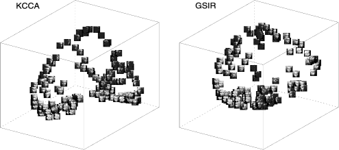
Figure 1: First 3 sufficient predictors by KCCA (left panel) and GSIR (right panel), computed from 558 training images, and evaluated on 140 testing images—faces data.

8.2 Data analysis

We first consider the faces data, available at http:// waldron.stanford.edu/isomap/datasets.html. This data set contains 698 images of the same sculpture of a face photographed at different angles and with different lighting directions. The predictor comprises $64\times 64$ image pixels (thus $p=4096$), and the response comprises horizontal rotation, vertical rotation and lighting direction measurements (thus $q=3$). We use this data to demonstrate that the first three sufficient predictors estimated by KCCA and GSIR can effectively capture the 3-variate response. We use $n=558$ of the images selected at random (roughly $80\%$) as training data, and the remaining $m=140$ images as testing data. For each method, we estimate the first three predictor functions from the training data, and evaluate them on the testing data. The left panel of Figure 1 is the perspective plot of the first three KCCA predictors evaluated on the 140 testing images, and the right panel is the counterpart for GSIR. We did not include KSIR in this comparison because in its proposed form it cannot handle multivariate responses. The perspective plots indicate that nearby regions in the 3-D cubes have similar patterns of left–right rotation, up–down rotation and lighting direction, while distant regions have discernibly different patterns. This reflects the ability of the three sufficient predictors to capture the 3-variate responses.

Figure 2: First 3 sufficient predictors by KSIR (upper-left panel), KCCA (upper-right panel) and GSIR (lower panel), computed on 1000 training images and evaluated on 1000 testing images—handwritten digits data.

Next, we apply KSIR, KCCA and GSIR to the handwritten digits data, available at http://www.cs.nyu.edu/~roweis/data.html. This data set contains 2000 images of $p=16\times 16$ pixels showing handwritten digits from 0 to 9—the response is thus categorical with 10 levels. We use 1000 images as training data and 1000 as testing data. Again, for each method we estimate the first three sufficient predictors on the training data, and evaluate them on the testing data. Results are presented in the three perspective plots in Figure 2—for visual clarity, these plots include only 100 randomly selected points from the 1000 in the testing data. The plots show that all three methods provide low-dimensional representations in which the digits are well separated.

9 Concluding remarks

In this article we described a novel and very general theory of sufficient dimension reduction. This theory allowed us to combine linear and nonlinear SDR into a coherent system, to link them with classical statistical sufficiency, and to subsume several existing nonlinear SDR methods into a unique framework.

Our developments thus revealed important and previously unexplored properties of SDR methods. For example, unbiasedness of various nonlinear extensions of SIR proposed in recent literature was proved under the stringent linear conditional mean assumption. We were able to show that these methods are all unbiased under virtually no assumption, and that GSIR is exhaustive under the completeness assumption. We were also able to show that nonlinear extensions of SIR are in general not exhaustive when completeness is not satisfied, and that in these cases GSAVE can recover a larger portion of the central class. These insights could not have been obtained without paralleling linear and nonlinear SDR as allowed by our new theory.

In addition to achieving theoretical synthesis and important insights on SDR methods, we introduced a new heteroscedastic conditional variance operator—which is more general than the (homoscedastic) conditional variance operator in Fukumizu, Bach and Jordan (2004, 2009). This operator was crucial to generalizing SAVE to the nonlinear GSAVE, and thus to exploit dependence information in the conditional variance to improve upon the performance of the nonlinear extensions of SIR. We have no doubt that the heteroschedastic conditional variance operator can be used to generate nonlinear extensions of other second-order SRD methods such as contour regression [Li, Zha and Chiaromonte (2005)], directional regression [Li and Wang (2007)], SIR-II [Li (1991)] and other F2M methods [Cook and Forzani (2009)]. These extensions will be the topic of future work.

More generally, it is our hope that the clarity and simplicity that classical notions lend to the formulation of dimension reduction, as well as the transparent parallels we were able to draw between linear and nonlinear SDR, will provide fertile grounds for much research to come.

As we put forward a general theory that encompasses both linear and nonlinear SDR, it is also important to point out that linear SDR has its special values that cannot be replaced by nonlinear SDR via kernel mapping, one of which is its preservation of the original coordinates and as a result its strong interpretability. For example, when mapped to higher dimension spaces, kernel methods can sometimes interpret difference in variances in the original coordinates as location separation in the transformed coordinates, which can be undesirable depending on the goal and emphasis of particular applications. For further discussion and an example of this point, see Li, Artemiou and Li (2011).

References

- Akaho (2001) {bincollection}[auto:STB—2013/01/29—08:09:18] \bauthor\bsnmAkaho, \bfnmS.\binitsS. (\byear2001). \btitleA kernel method for canonical correlation analysis. In \bbooktitleProceedings of the International Meeting of the Psychometric Society (IMPS2001). \bpublisherSpringer, \blocationTokyo. \bptokimsref \endbibitem
- Bach and Jordan (2002) {barticle}[mr] \bauthor\bsnmBach, \bfnmFrancis R.\binitsF. R. and \bauthor\bsnmJordan, \bfnmMichael I.\binitsM. I. (\byear2002). \btitleKernel independent component analysis. \bjournalJ. Mach. Learn. Res. \bvolume3 \bpages1–48. \biddoi=10.1162/153244303768966085, issn=1532-4435, mr=1966051 \bptnotecheck year\bptokimsref \endbibitem
- Bahadur (1954) {barticle}[mr] \bauthor\bsnmBahadur, \bfnmR. R.\binitsR. R. (\byear1954). \btitleSufficiency and statistical decision functions. \bjournalAnn. Math. Statist. \bvolume25 \bpages423–462. \bidissn=0003-4851, mr=0063630 \bptokimsref \endbibitem
- Baker (1973) {barticle}[mr] \bauthor\bsnmBaker, \bfnmCharles R.\binitsC. R. (\byear1973). \btitleJoint measures and cross-covariance operators. \bjournalTrans. Amer. Math. Soc. \bvolume186 \bpages273–289. \bidissn=0002-9947, mr=0336795 \bptokimsref \endbibitem
- Cook (1994) {bincollection}[auto:STB—2013/01/29—08:09:18] \bauthor\bsnmCook, \bfnmR. D.\binitsR. D. (\byear1994). \btitleUsing dimension-reduction subspaces to identify important inputs in models of physical systems. In \bbooktitle1994 Proceedings of the Section on Physical and Engineering Sciences \bpages18–25. \bpublisherAmer. Statist. Assoc., \blocationAlexandria, VA. \bptokimsref \endbibitem
- Cook (1998a) {bbook}[mr] \bauthor\bsnmCook, \bfnmR. Dennis\binitsR. D. (\byear1998a). \btitleRegression Graphics: Ideas for Studying Regressions Through Graphics. \bpublisherWiley, \blocationNew York. \biddoi=10.1002/9780470316931, mr=1645673 \bptokimsref \endbibitem
- Cook (1998b) {barticle}[mr] \bauthor\bsnmCook, \bfnmR. Dennis\binitsR. D. (\byear1998b). \btitlePrincipal Hessian directions revisited. \bjournalJ. Amer. Statist. Assoc. \bvolume93 \bpages84–94. \bptokimsref \endbibitem
- Cook (2007) {barticle}[mr] \bauthor\bsnmCook, \bfnmR. Dennis\binitsR. D. (\byear2007). \btitleFisher lecture: Dimension reduction in regression. \bjournalStatist. Sci. \bvolume22 \bpages1–40. \biddoi=10.1214/088342306000000682, issn=0883-4237, mr=2408655 \bptokimsref \endbibitem
- Cook and Critchley (2000) {barticle}[auto] \bauthor\bsnmCook, \bfnmR. D.\binitsR. D. and \bauthor\bsnmCritchley, \bfnmF.\binitsF. (\byear2000). \btitleIdentifying regression outliers and mixtures graphically. \bjournalJ. Amer. Statist. Assoc. \bvolume95 \bpages781–794. \bptokimsref \endbibitem
- Cook and Forzani (2009) {barticle}[mr] \bauthor\bsnmCook, \bfnmR. Dennis\binitsR. D. and \bauthor\bsnmForzani, \bfnmLiliana\binitsL. (\byear2009). \btitleLikelihood-based sufficient dimension reduction. \bjournalJ. Amer. Statist. Assoc. \bvolume104 \bpages197–208. \biddoi=10.1198/jasa.2009.0106, issn=0162-1459, mr=2504373 \bptokimsref \endbibitem
- Cook and Li (2002) {barticle}[mr] \bauthor\bsnmCook, \bfnmR. Dennis\binitsR. D. and \bauthor\bsnmLi, \bfnmBing\binitsB. (\byear2002). \btitleDimension reduction for conditional mean in regression. \bjournalAnn. Statist. \bvolume30 \bpages455–474. \biddoi=10.1214/aos/1021379861, issn=0090-5364, mr=1902895 \bptokimsref \endbibitem
- Cook, Li and Chiaromonte (2010) {barticle}[mr] \bauthor\bsnmCook, \bfnmR. Dennis\binitsR. D., \bauthor\bsnmLi, \bfnmBing\binitsB. and \bauthor\bsnmChiaromonte, \bfnmFrancesca\binitsF. (\byear2010). \btitleEnvelope models for parsimonious and efficient multivariate linear regression (with discussion). \bjournalStatist. Sinica \bvolume20 \bpages927–1010. \bptokimsref \endbibitem
- Cook and Ni (2005) {barticle}[mr] \bauthor\bsnmCook, \bfnmR. Dennis\binitsR. D. and \bauthor\bsnmNi, \bfnmLiqiang\binitsL. (\byear2005). \btitleSufficient dimension reduction via inverse regression: A minimum discrepancy approach. \bjournalJ. Amer. Statist. Assoc. \bvolume100 \bpages410–428. \biddoi=10.1198/016214504000001501, issn=0162-1459, mr=2160547 \bptokimsref \endbibitem
- Cook and Weisberg (1991) {barticle}[mr] \bauthor\bsnmCook, \bfnmR. D.\binitsR. D. and \bauthor\bsnmWeisberg, \bfnmS.\binitsS. (\byear1991). \btitleComment on “Sliced inverse regression for dimension reduction,” by K.-C. Li. \bjournalJ. Amer. Statist. Assoc. \bvolume86 \bpages328–332. \bptokimsref \endbibitem
- Duan and Li (1991) {barticle}[mr] \bauthor\bsnmDuan, \bfnmNaihua\binitsN. and \bauthor\bsnmLi, \bfnmKer-Chau\binitsK.-C. (\byear1991). \btitleA bias bound for least squares linear regression. \bjournalStatist. Sinica \bvolume1 \bpages127–136. \bidissn=1017-0405, mr=1101318 \bptokimsref \endbibitem
- Ferré and Yao (2003) {barticle}[mr] \bauthor\bsnmFerré, \bfnmL.\binitsL. and \bauthor\bsnmYao, \bfnmA. F.\binitsA. F. (\byear2003). \btitleFunctional sliced inverse regression analysis. \bjournalStatistics \bvolume37 \bpages475–488. \bptokimsref \endbibitem
- Fukumizu, Bach and Jordan (2004) {barticle}[mr] \bauthor\bsnmFukumizu, \bfnmKenji\binitsK., \bauthor\bsnmBach, \bfnmFrancis R.\binitsF. R. and \bauthor\bsnmJordan, \bfnmMichael I.\binitsM. I. (\byear2004). \btitleDimensionality reduction for supervised learning with reproducing kernel Hilbert spaces. \bjournalJ. Mach. Learn. Res. \bvolume5 \bpages73–99. \biddoi=10.1162/153244303768966111, issn=1532-4435, mr=2247974 \bptokimsref \endbibitem
- Fukumizu, Bach and Gretton (2007) {barticle}[mr] \bauthor\bsnmFukumizu, \bfnmKenji\binitsK., \bauthor\bsnmBach, \bfnmFrancis R.\binitsF. R. and \bauthor\bsnmGretton, \bfnmArthur\binitsA. (\byear2007). \btitleStatistical consistency of kernel canonical correlation analysis. \bjournalJ. Mach. Learn. Res. \bvolume8 \bpages361–383. \bidissn=1532-4435, mr=2320675 \bptokimsref \endbibitem
- Fukumizu, Bach and Jordan (2009) {barticle}[mr] \bauthor\bsnmFukumizu, \bfnmKenji\binitsK., \bauthor\bsnmBach, \bfnmFrancis R.\binitsF. R. and \bauthor\bsnmJordan, \bfnmMichael I.\binitsM. I. (\byear2009). \btitleKernel dimension reduction in regression. \bjournalAnn. Statist. \bvolume37 \bpages1871–1905. \biddoi=10.1214/08-AOS637, issn=0090-5364, mr=2533474 \bptokimsref \endbibitem
- Härdle, Hall and Ichimura (1993) {barticle}[mr] \bauthor\bsnmHärdle, \bfnmWolfgang\binitsW., \bauthor\bsnmHall, \bfnmPeter\binitsP. and \bauthor\bsnmIchimura, \bfnmHidehiko\binitsH. (\byear1993). \btitleOptimal smoothing in single-index models. \bjournalAnn. Statist. \bvolume21 \bpages157–178. \biddoi=10.1214/aos/1176349020, issn=0090-5364, mr=1212171 \bptokimsref \endbibitem
- Horn and Johnson (1985) {bbook}[mr] \bauthor\bsnmHorn, \bfnmRoger A.\binitsR. A. and \bauthor\bsnmJohnson, \bfnmCharles R.\binitsC. R. (\byear1985). \btitleMatrix Analysis. \bpublisherCambridge Univ. Press, \blocationCambridge. \bidmr=0832183 \bptokimsref \endbibitem
- Hsing and Ren (2009) {barticle}[mr] \bauthor\bsnmHsing, \bfnmTailen\binitsT. and \bauthor\bsnmRen, \bfnmHaobo\binitsH. (\byear2009). \btitleAn RKHS formulation of the inverse regression dimension-reduction problem. \bjournalAnn. Statist. \bvolume37 \bpages726–755. \biddoi=10.1214/07-AOS589, issn=0090-5364, mr=2502649 \bptokimsref \endbibitem
- Ichimura and Lee (1991) {bincollection}[mr] \bauthor\bsnmIchimura, \bfnmHidehiko\binitsH. and \bauthor\bsnmLee, \bfnmLung Fei\binitsL. F. (\byear1991). \btitleSemiparametric least squares estimation of multiple index models: Single equation estimation. In \bbooktitleNonparametric and Semiparametric Methods in Econometrics and Statistics (Durham, NC, 1988) (\beditorW. A. Barnett, \beditorJ. L. Powell and \beditorG. Tauchen, eds.) \bpages3–49. \bpublisherCambridge Univ. Press, \blocationCambridge. \bidmr=1174973 \bptokimsref \endbibitem
- Lee, Li and Chiaromonte (2013) {bmisc}[auto:STB—2013/01/29—08:09:18] \bauthor\bsnmLee, \bfnmK. Y.\binitsK. Y., \bauthor\bsnmLi, \bfnmB.\binitsB. and \bauthor\bsnmChiaromonte, \bfnmF.\binitsF. (\byear2013). \bhowpublishedSupplement to “A general theory for nonlinear sufficient dimension reduction: Formulation and estimation.” DOI:\doiurl10.1214/12-AOS1071SUPP. \bptokimsref \endbibitem
- Lehmann (1981) {barticle}[mr] \bauthor\bsnmLehmann, \bfnmE. L.\binitsE. L. (\byear1981). \btitleAn interpretation of completeness and Basu’s theorem. \bjournalJ. Amer. Statist. Assoc. \bvolume76 \bpages335–340. \bidissn=0162-1459, mr=0624335 \bptokimsref \endbibitem
- Li (1991) {barticle}[mr] \bauthor\bsnmLi, \bfnmKer-Chau\binitsK.-C. (\byear1991). \btitleSliced inverse regression for dimension reduction. \bjournalJ. Amer. Statist. Assoc. \bvolume86 \bpages316–342. \bidissn=0162-1459, mr=1137117 \bptokimsref \endbibitem
- Li (1992) {barticle}[auto:STB—2013/01/29—08:09:18] \bauthor\bsnmLi, \bfnmKer-Chau\binitsK.-C. (\byear1992). \btitleOn principal Hessian directions for data visualization and dimension reduction: Another application of Stein’s lemma. \bjournalJ. Amer. Statist. Assoc. \bvolume86 \bpages316–342. \bptokimsref \endbibitem
- Li, Artemiou and Li (2011) {barticle}[auto:STB—2013/01/29—08:09:18] \bauthor\bsnmLi, \bfnmB.\binitsB., \bauthor\bsnmArtemiou, \bfnmA.\binitsA. and \bauthor\bsnmLi, \bfnmL.\binitsL. (\byear2011). \btitlePrincipal support vector machines for linear and nonlinear sufficient dimension reduction. \bjournalAnn. Statist. \bvolume9 \bpages3182–3210. \bptokimsref \endbibitem
- Li, Chun and Zhao (2012) {barticle}[auto:STB—2013/01/29—08:09:18] \bauthor\bsnmLi, \bfnmB.\binitsB., \bauthor\bsnmChun, \bfnmH.\binitsH. and \bauthor\bsnmZhao, \bfnmH.\binitsH. (\byear2012). \btitleSparse estimation of conditional graphical models with application to gene networks. \bjournalJ. Amer. Statist. Assoc. \bvolume107 \bpages152–167. \bptokimsref \endbibitem
- Li and Duan (1989) {barticle}[mr] \bauthor\bsnmLi, \bfnmKer-Chau\binitsK.-C. and \bauthor\bsnmDuan, \bfnmNaihua\binitsN. (\byear1989). \btitleRegression analysis under link violation. \bjournalAnn. Statist. \bvolume17 \bpages1009–1052. \biddoi=10.1214/aos/1176347254, issn=0090-5364, mr=1015136 \bptokimsref \endbibitem
- Li and Wang (2007) {barticle}[mr] \bauthor\bsnmLi, \bfnmBing\binitsB. and \bauthor\bsnmWang, \bfnmShaoli\binitsS. (\byear2007). \btitleOn directional regression for dimension reduction. \bjournalJ. Amer. Statist. Assoc. \bvolume102 \bpages997–1008. \biddoi=10.1198/016214507000000536, issn=0162-1459, mr=2354409 \bptokimsref \endbibitem
- Li, Zha and Chiaromonte (2005) {barticle}[mr] \bauthor\bsnmLi, \bfnmBing\binitsB., \bauthor\bsnmZha, \bfnmHongyuan\binitsH. and \bauthor\bsnmChiaromonte, \bfnmFrancesca\binitsF. (\byear2005). \btitleContour regression: A general approach to dimension reduction. \bjournalAnn. Statist. \bvolume33 \bpages1580–1616. \biddoi=10.1214/009053605000000192, issn=0090-5364, mr=2166556 \bptokimsref \endbibitem
- Wu (2008) {barticle}[mr] \bauthor\bsnmWu, \bfnmHan-Ming\binitsH.-M. (\byear2008). \btitleKernel sliced inverse regression with applications to classification. \bjournalJ. Comput. Graph. Statist. \bvolume17 \bpages590–610. \biddoi=10.1198/106186008X345161, issn=1061-8600, mr=2528238 \bptokimsref \endbibitem
- Wu, Liang and Mukherjee (2008) {bmisc}[auto:STB—2013/01/29—08:09:18] \bauthor\bsnmWu, \bfnmQ.\binitsQ., \bauthor\bsnmLiang, \bfnmF.\binitsF. and \bauthor\bsnmMukherjee, \bfnmS.\binitsS. (\byear2008). \btitleRegularized sliced inverse regression for kernel models. Technical report, Duke Univ., Durham, NC. \bptokimsref \endbibitem
- Ye and Weiss (2003) {barticle}[auto:STB—2013/01/29—08:09:18] \bauthor\bsnmYe, \bfnmZ.\binitsZ. and \bauthor\bsnmWeiss, \bfnmR. E.\binitsR. E. (\byear2003). \btitleUsing the bootstrap to select one of a new class of dimension reduction methods. \bjournalJ. Amer. Statist. Assoc. \bvolume98 \bpages968–979. \bptokimsref \endbibitem
- Yeh, Huang and Lee (2009) {barticle}[auto:STB—2013/01/29—08:09:18] \bauthor\bsnmYeh, \bfnmY. R.\binitsY. R., \bauthor\bsnmHuang, \bfnmS. Y.\binitsS. Y. and \bauthor\bsnmLee, \bfnmY. Y.\binitsY. Y. (\byear2009). \btitleNonlinear dimension reduction with kernel sliced inverse regression. \bjournalIEEE Transactions on Knowledge and Data Engineering \bvolume21 \bpages1590–1603. \bptokimsref \endbibitem
- Yin, Li and Cook (2008) {barticle}[mr] \bauthor\bsnmYin, \bfnmXiangrong\binitsX., \bauthor\bsnmLi, \bfnmBing\binitsB. and \bauthor\bsnmCook, \bfnmR. Dennis\binitsR. D. (\byear2008). \btitleSuccessive direction extraction for estimating the central subspace in a multiple-index regression. \bjournalJ. Multivariate Anal. \bvolume99 \bpages1733–1757. \biddoi=10.1016/j.jmva.2008.01.006, issn=0047-259X, mr=2444817 \bptokimsref \endbibitem
- Zhu and Li (2011) {barticle}[pbm] \bauthor\bsnmZhu, \bfnmHongjie\binitsH. and \bauthor\bsnmLi, \bfnmLexin\binitsL. (\byear2011). \btitleBiological pathway selection through nonlinear dimension reduction. \bjournalBiostatistics \bvolume12 \bpages429–444. \biddoi=10.1093/biostatistics/kxq081, issn=1468-4357, pii=kxq081, pmid=21252081 \bptokimsref \endbibitem