A new approach to multi-modal diffusions
with applications to protein folding

Summary

This article demonstrates that flexible and statistically tractable multi-modal diffusion models can be attained by transformation of simple well-known diffusion models such as the Ornstein-Uhlenbeck model, or more generally a Pearson diffusion. The transformed diffusion inherits many properties of the underlying simple diffusion including its mixing rates and distributions of first passage times. Likelihood inference and martingale estimating functions are considered in the case of a discretely observed bimodal diffusion. It is further demonstrated that model parameters can be identified and estimated when the diffusion is observed with additional measurement error. The new approach is applied to molecular dynamics data in form of a reaction coordinate of the small Trp-zipper protein, for which the folding and unfolding rates are estimated. The new models provide a better fit to this type of protein folding data than previous models because the diffusion coefficient is state-dependent.

Key words: diffusion; mean passage time; measurement error; martingale estimating function; multi-modality; protein folding; stochastic differential equation.

1 Introduction

In this article we propose a new class of stationary stochastic differential equation models that have multi-modal invariant distributions. These models are useful for modeling dynamical systems that switch randomly between two or more regimes. As an example, we consider molecular dynamics data in form of a protein reaction coordinate with two regimes corresponding to the folded and unfolded state of the protein, respectively. Essentially protein folding happens in a high-dimensional space, but a remarkable consequence of the energy landscape theory is that folding is essentially a low dimensional process as it happens down a folding funnel. It has been suggested that folding can be accurately captured by one or a few suitably chosen protein reaction coordinates (that is, univariate characteristics of the protein) with diffusive dynamics along the folding funnel, see [Socci, Onuchic & Wolynes (1996], [Das et al. (2006], and the references therein. Note, however, that applications of bimodal diffusions are not limited to the study of molecular dynamics. Other applications of bimodal diffusion are as models of the global climate where the two regimes could be a cold and a hot climate as in [Imkeller & Pavlyukevich (2002], and as financial models of e.g. interest rates subject to changes in the underlying financial and economic mechanisms as in [Aït-Sahalia (1996].

Traditionally bimodal diffusion processes have been constructed by a stochastic differential equation with additive noise for a process moving in a double-well potential, i.e. a stochastic differential equation of the form

$$dY_{t}=-V^{\prime}(Y_{t})dt+\sigma^{2}dB_{t},$$ (1)

where $\{B_{t}\}$ is a Wiener process and $V$ is a potential with two valleys. Under the condition that $V(y)$ goes to infinity at the boundaries of the state space and that the function $h(y)=\exp\{-2V(y)/\sigma^{2}\}$ is integrable on the state space, $\{Y_{t}\}$ is ergodic with invariant density proportional to $h(y)$. An often studied example is given by the potential $V(y)=\theta y^{2}(y^{2}-2)$ with $\theta>0$, for which the drift is $-4\theta(y^{3}-y)=-4\theta y(y+1)(y-1)$. This simple potential has wells of the same depths at 1 and -1 and is symmetric around a separating potential barrier at 0. The related diffusion is ergodic with invariant density proportional to $\exp\{-2\theta(y^{4}-2y^{2})\}$. It is easy to generalize this model to models with wells at other points that need not be symmetric around the separating potential barrier. The double well potential models are the state of the art in the analysis of protein reaction coordinates. That is, constant diffusion is usually assumed and used in the estimation of the protein folding rates, see e.g. [Socci, Onuchic & Wolynes (1996]. A more complex model of molecular dynamics was presented in [Pokern, Stuart & Wiberg (2009] who used a partially observed hypoelliptical diffusion to model the dihedral angle in a butane molecule. Still this model assumes a constant diffusion coefficient which may conflict with that of the data. More recently evidence of non-constant diffusion in protein reaction coordinates have been reported in several articles. [Best & Hummer (2010] discusses these findings and their implications for the assessment of protein folding rates.

Our new class of bimodal diffusions is obtained by applying particular transformations to simple well-known diffusions such as the Ornstein-Uhlenbeck process or a general Pearson diffusion; see [Forman & Sørensen (2008]. This leads to diffusion models with nonlinear drift and non-constant diffusion coefficients that are still highly tractable both from a statistical and a computational point of view. A major point of this article is that many properties of diffusions are preserved by transformation. These include stationarity, mixing properties, and distributions of first passage times. Also the eigenvalues of the infinitesimal generator of the diffusion are preserved by the transformation, and eigenfunctions transform in a straightforward way. This facilitates efficient approximate likelihood inference by means of e.g. the explicit martingale estimating functions proposed by [Kessler & Sørensen (1999]. In the rare cases where the likelihood function of a diffusion is explicitly known, this is also the case for any of its transformations. Similarly to the double well potential models, our new diffusion models allow for great flexibility in the modeling of the invariant marginal distribution. Thus, the new bimodal diffusion models provide a useful extension of the class of bimodal diffusion models.

An alternative to the stochastic differential equation approach is to model each regime separately and to let the shifts between the models be determined by an underlying finite-state process such as a hidden Markov model or Markov state model. These models are widely employed as models of protein folding, see [Prinz et al. (2011] for a review, although it is recognized that the models are inadequate in describing the more gradual transition between states which is the de facto behaviour of many proteins. Latent Markov state models are also very popular in financial and econometric applications, see [Lange & Rahbek (2009] for an overview. However, a latent state model is too complex and difficult to interpret if what is observed is not two different dynamical systems, but is really the same dynamical system that just has the property that it can be in two different regimes. A multi-modal diffusion has local attractions points corresponding to its regimes and moves between them in a continuous and random way. Apart from the conceptual advantage and the simpler model, other advantages of a multi-modal diffusion over two separate models is that the stationary marginal density in a succinct way contains important information about the regimes: the relative size of the modes reflect the time spent in each mode, and the peakedness and broadness of the modes reflect the volatility of the regimes. Moreover, explicit formulae for mean passage times allows for precise calculation of the time spent in each regime and the probability of switching from one regime to another.

The article is organized as follows: Section 2 is devoted to the construction of our multi-modal diffusion model. We investigate the properties of these model and contrast them to other existing bimodal diffusions, the double-well potential models in particular. In Section 3 we discuss inference for the new class of bimodal diffusions emphasizing approximate likelihood inference based on martingale estimating functions. Inference is further discussed when the bimodal diffusion is observed with measurement error. In Section 4 we apply a bimodal diffusion model to molecular dynamics data in form of a reaction coordinate of the small Trp-zipper protein. Upon adjusting for measurement error we arrive at estimated folding rates that are realistic for this kind of protein. Section 5 concludes.

2 Multi-modal diffusions by transformation

2.1 Multi-modal distributions

As a starting point we consider a bimodal density $f$. For instance, $f$ could be the invariant density of the double-well potential diffusion (1) or the mixture of two unimodal densities $f_{1}$ and $f_{2}$,

$$f=\alpha\cdot f_{1}+(1-\alpha)\cdot f_{2},\quad 0<\alpha<1.$$ (2)

This density will be the marginal invariant density of our bimodal diffusion. As our main example, we consider the bimodal normal mixture density $\alpha\cdot\phi(\cdot;\mu_{1},\sigma_{1}^{2})+(1-\alpha)\phi(\cdot;\mu_{2},\sigma_{2}^{2})$, where the mean parameters $\mu_{1}$ and $\mu_{2}$ determine the location of the two modes and the variance parameters $\sigma_{1}^{2}$ and $\sigma_{2}^{2}$ determine the broadness of each mode. Some instances of this density are shown in Figure 1 below. The bimodal normal density fits the protein reaction coordinate data in our case study (Section 4) well. In other applications it might be more relevant to consider densities $f_{1}$ and $f_{2}$ that are constrained to a bounded interval (this is the case for certain protein reaction coordinates), or that are heavy-tailed or skew (e.g. financial data).

Note that if the mode points of the two unimodal densities are not located sufficiently far apart, then the mode points of the bimodal density are not identical to the mode points of the unimodal densities, or the mixture density might not be bimodal at all. This, however, is not a problem when applying the model to data where bimodality is manifest. Further, for particular choices of parameters, the bimodality of (2) can easily be checked; its mode points can be found numerically.

An important point of the paper is that multi-modal diffusions with more than two regimes can also be constructed by the method presented in this section by simply choosing for $f$ a multi-modal density. For instance, a tri-modal diffusion is obtained for $f=\alpha_{1}f_{1}+\alpha_{2}f_{2}+\alpha_{3}f_{3}$, $\alpha_{1},\alpha_{2},\alpha_{3}\in(0,1)$, $\alpha_{1}+\alpha_{2}+\alpha_{3}=1$, where $f_{i}$, $i=1,2,3$, are unimodal probability densities whose modes are sufficiently separated. It is merely to simplify the presentation that we describe only the bimodal model in detail.

2.2 Bimodal diffusions

In order to model a bimodal (multi-modal) diffusion, we initially consider a stationary diffusion of general form,

$$dX_{t}=\mu(X_{t})dt+\sigma(X_{t})dB_{t},$$ (3)

where $\{B_{t}\}$ is a Wiener process, and where we assume that the coefficients are sufficiently regular to ensure that a unique weak solution exists for any given initial condition. In principle $\{X_{t}\}$ could be any diffusion, but we aim to construct bimodal diffusions for which statistical inference is relatively easy, so we are interested in cases where the diffusion $\{X_{t}\}$ is analytically tractable. This is for instance the case if $\{X_{t}\}$ is an ergodic Pearson diffusion as considered by [Forman & Sørensen (2008], see in addition [Wong (1964] for an early account on these processes.

Recall that a stationary solution $\{X_{t}\}$ to the stochastic differential equation exists if

$$\int_{x^{\#}}^{r}s(x)dx=\int^{x^{\#}}_{\ell}s(x)dx=\infty\quad\textnormal{ and }\quad\int_{\ell}^{r}[s(x)\sigma^{2}(x)]^{-1}dx<\infty.$$

where the state space is $(\ell,r)$ ($-\infty\leq\ell<r\leq\infty$), $x^{\#}\in(\ell,r)$ is arbitrary, and $s(x)$ is the density of the scale measure

$$s(x)=\exp\left(-2\int_{x^{\#}}^{x}\frac{\mu(y)}{\sigma^{2}(y)}dy\right),\ \ \ x\in(\ell,r).$$ (4)

Under these conditions the diffusion $\{X_{t}\}$ is ergodic with invariant probability density given by $\pi(x)=(\int_{\ell}^{r}\{s(y)\sigma^{2}(y)\}^{-1}dy)^{-1}\cdot\{s(x)\sigma^{2}(x)\}^{-1}$, see [Karlin & Taylor (1981].

Let $\Pi$ denote the cumulative distribution function of the invariant distribution of the diffusion $\{X_{t}\}$ given by (3), then a stationary diffusion with bimodal (multi-modal) invariant density can be obtained by transforming $\{X_{t}\}$ with the transformation

$$\operatorname{\tau}=F^{-1}\circ\Pi$$

where $F^{-1}$ is the quantile function of the bimodal (multi-modal) density. The cumulative distribution function of the bimodal mixture density (2) is obviously given by $F(y)=\alpha F_{1}(y)+(1-\alpha)F_{2}(y)$, where $F_{1}$ and $F_{2}$ are the cumulative distribution functions of the two unimodal distributions, so for practical purposes $F^{-1}$ can easily be computed. The dynamics of the transformed diffusion $\{Y_{t}\}=\{\operatorname{\tau}(X_{t})\}$ are given by the stochastic differential equation,

$$dY_{t} = \mu^{\operatorname{\tau}}(Y_{t})+\sigma^{\operatorname{\tau}}(Y_{t})dB_{t},$$ (5)

$$\mu^{\operatorname{\tau}}(y) = \frac{2\mu(\operatorname{\tau}^{-1}y)\pi(\operatorname{\tau}^{-1}y)+\sigma^{2}(\operatorname{\tau}^{-1}y)\pi^{\prime}(\operatorname{\tau}^{-1}y)}{2f(y)}-\frac{\sigma^{2}(\operatorname{\tau}^{-1}y)\pi^{2}(\operatorname{\tau}^{-1}y)f^{\prime}(y)}{2f(y)^{3}}$$

$$\sigma^{\operatorname{\tau}}(y) = \frac{\pi(\operatorname{\tau}^{-1}y)\sigma(\operatorname{\tau}^{-1}y)}{f(y)}$$

with $\operatorname{\tau}^{-1}=\Pi^{-1}\circ F$ and where we have abbreviated $\operatorname{\tau}^{-1}(y)$ as $\operatorname{\tau}^{-1}y$.

Figure 1: Densities, drifts and diffusion coefficients of transformed Ornstein-Uhlenbeck processes (7) with parameters $\beta=1$ and invariant bimodal normal mixture densities given by $f(y)=\alpha\phi(y;\mu_{1},\sigma_{1})+(1-\alpha)\phi(y;\mu_{1},\sigma_{2})$ with $\sigma_{1}=\sigma_{2}=1$ and $-\mu_{1}=\mu_{2}=\mu$ varying as $\mu=1.05$ (solid lines), $\mu=1.5$ (dashed lines), or $\mu=2$ (dotted lines). The upper panel shows symmetric densities ($\alpha=0.5$) and the lower panel asymmetric densities ($\alpha=0.75$).

Example: Transformation of the stationary Ornstein-Uhlenbeck process,

$$dX_{t}=-\nu X_{t}dt+\sqrt{2\nu}dB_{t}$$ (6)

with invariant distribution equal to the standard normal distribution and autocorrelation function $\rho(t)=e^{-\nu t}$, yields the diffusion

$$dY_{t}=-2\nu\cdot\left(\frac{\operatorname{\tau}^{-1}(Y_{t})\varphi(\operatorname{\tau}^{-1}Y_{t})}{f(Y_{t})}+\frac{\varphi^{2}(\operatorname{\tau}^{-1}Y_{t})f^{\prime}(Y_{t})}{2f(Y_{t})^{3}}\right)dt+\frac{\sqrt{2\nu}\varphi(\operatorname{\tau}^{-1}Y_{t})}{f(Y_{t})}dB_{t},$$ (7)

where $\operatorname{\tau}^{-1}=\Phi^{-1}\circ F$, and where $\varphi$ and $\Phi$ denote the density and the cumulative distribution function, respectively, of the standard normal distribution. Drifts and diffusion coefficients of some transformed Ornstein-Uhlenbeck process are shown in Figure 1. Note that the diffusion coefficients of the transformed Ornstein-Uhlenbeck processes peaks in-between the modes, which makes the model a good candidate for protein reaction coordinates such as the one studied in Section 4. $\bullet$

Both the transformed Ornstein-Uhlenbeck process (7) and the general transformed diffusion (5) inherits many properties from the simple diffusion $\{X_{t}\}$. The following results are straight-forward and thus stated without proof.

Proposition 2.1

Let $f$ be the bimodal mixture density defined by (2), and $\{X_{t}\}$ and $\{Y_{t}\}$ the diffusions specified by (3) and (5), respectively, then the following hold true.

1. If the densities $f_{1}$ and $f_{2}$ distributions have finite $k^{\prime}th$ order moments $\mu_{k}(f_{1})$ and $\mu_{k}(f_{2})$, then so has the bimodal mixture density; $\mu_{k}(f)=\alpha\mu_{k}(f_{1})+(1-\alpha)\mu_{k}(f_{2})$. In particular, the mean and variance are $E(f)=\alpha E(f_{1})+(1-\alpha)E(f_{2})$ and

   $$\operatorname{Var}(f)=\alpha\operatorname{Var}(f_{1})+(1-\alpha)\operatorname{Var}(f_{2})+\alpha(1-\alpha)\{E(f_{1})-E(f_{2})\}^{2}.$$

2. If $\{X_{t}\}$ is stationary and ergodic, then so is $\{Y_{t}\}$.

3. The ($\alpha$, $\beta$ and $\rho$) mixing coefficients of $\{X_{t}\}$ and $\{Y_{t}\}$ satisfy $\kappa_{t}(X)=\kappa_{t}(Y)$, where $\kappa$ is either of $\alpha$, $\beta$, or $\rho$. In particular if $\{X_{t}\}$ is $\kappa$-mixing (i.e. $\kappa_{t}\to 0$ as $t\to\infty$), then so is $\{Y_{t}\}$. We refer to [Doukhan (1994] for further explanation.

4. If $g$ is an eigenfunction for the infinitesimal generator of the diffusion $\{X_{t}\}$ with eigenvalue $\lambda$, then $g\circ\operatorname{\tau}^{-1}$ is an eigenfunction of the generator of $\{Y_{t}\}$ with the same eigenvalue (the infinitesimal generator of the diffusion (3) is the differential operator $\mathcal{L}=\mu\cdot\frac{d}{dx}+\frac{\sigma^{2}}{2}\frac{d^{2}}{dx^{2}}$, see [Karlin & Taylor (1981]. In particular it holds that $E\{g(\operatorname{\tau}^{-1}Y_{t})|Y_{0}\}=e^{-\lambda t}g(\operatorname{\tau}^{-1}Y_{0})$ under mild regularity conditions, see [Kessler & Sørensen (1999].

5. If $\{p(x|x^{\prime},\Delta)\}$ denote the transition densities of $\{X_{t}\}$ (i.e. $p(x|x^{\prime},\Delta)$ is the conditional density of $X_{t+\Delta}$ given $X_{t}=x^{\prime}$), then the transition densities $\{q(y|y^{\prime},\Delta)\}$ of $\{Y_{t}\}$ are given by $q(y|y^{\prime},\Delta)=p(\operatorname{\tau}^{-1}y|\operatorname{\tau}^{-1}y^{\prime},\Delta)\cdot f(y)/\pi(\operatorname{\tau}^{-1}y)$.

One of the merits of the bimodal diffusion model is its capability of quantifying the shifts between its two regimes. These can be described by the passage times of the diffusion. We make use of this to estimate the folding and unfolding rate of the small Trp-zipper protein in Section 4.

The first passage time to $b$ of the general diffusion (3) is defined by

$$T_{X}(b)=\inf\{t\geq 0\colon X_{t}=b\}$$

and given that $a<b$ the mean passage time from $a$ to $b$ is equal to

$$E(T_{X}(b)|X_{0}=a)=2\int_{\ell}^{a}\pi(x)dx\cdot\int_{a}^{b}s(x)dx+\int_{a}^{b}\pi(x)\int_{x}^{b}s(y)dydx$$

where $s(x)$ is the scale density given by (4), see [Karlin & Taylor (1981]. Similarly, for the passage from $b$ to $a$ it holds that

$$E(T_{X}(a)|X_{0}=b)=2\int_{b}^{r}\pi(x)dx\cdot\int_{a}^{b}s(x)dx+\int_{a}^{b}\pi(x)\int_{a}^{x}s(y)dydx.$$

The distributions of the passage times of the transformed diffusion are directly related to those of the underlying simple diffusion, as obviously $T_{Y}(b)=T_{X}(\operatorname{\tau}^{-1}b)$. Hence we have the following result:

Proposition 2.2

Denote by $T_{X}$ a first passage time of the diffusion (3) and by $T_{Y}$ a first passage time of the transformed diffusion (5), then for any $a,b\in(\ell,r)$:

$$(T_{Y}(b)|Y_{0}=a)\stackrel{{\scriptstyle\mathcal{D}}}{{=}}(T_{X}(\operatorname{\tau}^{-1}b)|X_{0}=\operatorname{\tau}^{-1}a),\hskip 5.69054pt(T_{Y}(a)|Y_{0}=b)\stackrel{{\scriptstyle\mathcal{D}}}{{=}}(T_{X}(\operatorname{\tau}^{-1}a)|X_{0}=\operatorname{\tau}^{-1}b).$$ (8)

Example: The mean passage times of the transformed Ornstein-Uhlenbeck process, (7), between points $a<b$ are given by

$$E(T_{Y}(b)|Y_{0}=a)=\frac{\sqrt{2\pi}}{\nu}\int_{\operatorname{\tau}^{-1}a}^{\operatorname{\tau}^{-1}b}\Phi(x)e^{x^{2}/2}dx$$ (9)

and

$$E(T_{Y}(a)|Y_{0}=b)=\frac{\sqrt{2\pi}}{\nu}\int_{\operatorname{\tau}^{-1}a}^{\operatorname{\tau}^{-1}b}\{1-\Phi(x)\}e^{x^{2}/2}dx.$$ (10)

where $\Phi$ is the cumulative distribution function of the standard normal distribution.

In fact the passage times of the Ornstein-Uhlenbeck can be described in greater detail as it is possible to find analytical expressions of their densities, see [Alili, Patie & Pedersen (2004] and the references therein. Although involving series expansions and special functions, the densities can be computed by means of designated software. This could potentially be used to further describe the folding and unfolding of the small Trp-zipper protein studied in Section 4. $\bullet$

2.3 Comparison to other bimodal diffusion models

Double well potential models such as (1) considered in the introduction are the state-of-the-art models for protein reaction coordinates. It should be noted that the double-well potential diffusion model is quite flexible and can be made to match any particular bimodal density $f$ by specifying the potential as $V(x)=-\frac{\sigma^{2}}{2}\log f(x)$. One might suspect that a diffusion of our type is a transformation of yet another diffusion with constant diffusion coefficient that moves in a double-well potential, and that this is the real underlying cause for the bimodality. However, we will demonstrate that this is not the case: Suppose a diffusion $\{Y_{t}\}$ with bimodal invariant density $f$ is constructed by transformation of a simple diffusion $\{X_{t}\}$ by the method in the previous section. To any diffusion of the general form (3) corresponds a unique transformation to a diffusion $\{\widetilde{X}\}$ with constant diffusion coefficient, the so-called Lamperti transformation, $\widetilde{X}_{t}=\int_{x^{\#}}^{X_{t}}\{\sigma(y)\}^{-1}dy$, see e.g. [Iacus (2008]. Since $\sigma^{\operatorname{\tau}}(y)=\sigma\{\operatorname{\tau}^{-1}y\}\cdot\operatorname{\tau}^{\prime}\{\operatorname{\tau}^{-1}y\}$, it is not difficult to show that when applying the Lamperti transformation of the bimodal transformed diffusion $\{Y_{t}\}=\{\tau(X_{t})\}$ to this process, then the resulting process is identical to $\{\widetilde{X}_{t}\}$, which is completely unrelated to the bimodal density $f$. Our approach to bimodal diffusions is thus genuinely different from the double-well potential models. In the new models the bimodality is not caused by a double-well potential; rather the bimodality is the product of an interplay between the smooth motion given by the drift and the random fluctuations given by the state-dependent diffusion coefficient.

[Aït-Sahalia (1996] proposed a general nonlinear diffusion model specified by,

$$dX_{t}=(\alpha_{-1}X_{t}^{-1}+\alpha_{0}+\alpha_{1}X_{t}+\alpha_{2}X_{t}^{2})dt+\sqrt{\beta_{0}+\beta_{1}X_{t}+\beta_{2}X_{t}^{\gamma}}dB_{t},$$ (11)

The parameter constraints under which (11) is stationary and ergodic are complicated and we will not quote them here. The nonlinear diffusion model may display bimodality, but at the same time it contains simple unimodal models such as the Ornstein-Uhlenbeck process. The nonlinear bimodal diffusion process produces bimodality in the same way as our new model does, although in the model (11) most of the action is in the drift. In comparison with the other classes of models, the nonlinear diffusion (11) has the disadvantage that in its general form it does not admit simple explicit estimating functions, like our transformed diffusions do, and that analytical likelihood approximations do not simplify for (11) as they do for the double-well potential models, see Section 3 below. Also the nonlinear diffusion (11) is not quite as easy to simulate as the other models.

In regard to the protein folding problem, any of the three classes of models may be relevant as different kinds of reaction coordinates display varying patterns of diffusion. For instance, our new model seems apt at modeling reaction coordinates that measure fluctuations in Cartesian configuration space for which diffusion is increased in-between modes, e.g. as in [Best & Hummer (2010], whereas the nonlinear diffusion model is a better model for a reaction coordinates in which diffusion decrease monotonically towards the folded state, e.g. as in [Chahine et al. (2007].

We end this Section by remarking that bimodality can also be produced solely by effects of the random fluctuations determined by a state dependent diffusion coefficient, as is clear from the following example. Suppose $f$ is a bimodal density function for which the support is the real line. Then the diffusion given by

$$dX_{t}=\frac{\sigma}{\sqrt{f(X_{t})}}dB_{t}$$ (12)

is ergodic with invariant density $f$, see e.g. [Bibby & Sørensen (1997]. The bimodality is produced by the fact that near the two mode-points the random fluctuations are relatively small, so that the process tends to stay near these points. When the process is far from the mode-points, the random fluctuations are large and will quickly send the process to other parts of the state space. Thus the same bimodal invariant distribution can be attained for diffusions with very different drift and diffusion coefficients and by completely different mechanisms. Our approach combines the mechanisms of the double-well potential diffusions (motion in an energy landscape), and of the pure diffusion models (12) (state-dependent random fluctuations).

3 Statistical inference:

3.1 Discretely observed diffusion

In what follows we discuss inference for a discretely observed multi-modal diffusion of the type constructed in Section 2. We assume that observations are made at equidistant time points $t_{i}=i\Delta$ for $i=0,\ldots,N$, where $\Delta^{-1}>0$ is the sampling frequency. We denote the observations by $y_{0},\ldots,y_{N}$. Further, we assume that the distribution of the underlying simple diffusion $\{X_{t}\}$ is dependent on a $p_{1}$-dimensional vector of parameters $\nu$ and that the bimodal density $f_{\psi}$ is dependent on a $p_{2}$-dimensional vector of parameters $\psi$.

Likelihood estimation
Likelihood estimation is our preferred means of inference, but it is unfortunately rarely the case that the likelihood function of a diffusion process is explicitly known. Therefore inference for diffusion models is usually best carried out by means of approximate likelihood methods. A noteworthy exception is the Ornstein-Uhlenbeck process and transformations of it, for which the likelihood functions is explicitly known. In particular this is true for our bimodal transformation of the Ornstein-Uhlenbeck process for which the likelihood function is given by

$$L_{n}(\psi,\nu)=\prod_{i=0}^{n-1}\frac{1}{\sqrt{1-e^{-2\nu\Delta}}}\varphi\left(\frac{\operatorname{\tau}^{-1}_{\psi,\nu}y_{i+1}-e^{-\nu\Delta}\operatorname{\tau}^{-1}_{\psi,\nu}y_{i}}{\sqrt{1-e^{-2\nu\Delta}}}\right)\frac{f_{\psi}(y_{i+1})}{\varphi(\operatorname{\tau}^{-1}_{\psi,\nu}y_{i+1})},$$

where $\varphi$ denotes the standard normal density function.

Approximate likelihood inference is applicable to many diffusions by using [Aït-Sahalia (2002]’s analytical approximation to the likelihood function. In a simulation study by [Jensen & Poulsen (2002] it was demonstrated that this particular likelihood approximation is superior to other approximate likelihood methods both in terms of computing time and in terms of numerical accuracy. An implementation of this method can be found in [Iacus (2008]. The first step in the analytical likelihood approximation is to compute the Lamperti transform of the diffusion, see Section 2. Hence, with likelihood inference in mind it is desirable to choose an underlying diffusion with a simple Lamperti transform. As demonstrated in Section 2 the process obtained when applying the Lamperti transform is invariant under transformation. Likelihood inference is therefore a natural choice for inference in the double-well potential model (1). Since the diffusion coefficient is already constant, the first step in [Aït-Sahalia (2002]’s approximation can be skipped.

Martingale estimating functions
Martingale estimating functions are another way of approximating likelihood inference. Specifically, they are unbiased approximations to the score function, see [Bibby, Jacobsen & Sørensen (2010]. For instance the quadratic martingale estimating function, [Bibby & Sørensen (1995], is a simple, yet often highly efficient, means for obtaining parameter estimates in a diffusion model, see [Sørensen (2012a]. If $H_{N}(\psi,\nu)$ denotes a general estimating function for the diffusion model (5), then an estimate $(\hat{\psi},\hat{\nu})$ is obtained by solving the estimating equation $H_{N}(\psi,\nu)=0$.

For the Pearson diffusions we can not only find explicit expressions for moments and conditional moments (to the extent these exist), but also explicit polynomial eigenfunctions for the infinitesimal generator. We can therefore find explicit eigenfunctions for transformations of Pearson diffusions as shown in Proposition 2.1. This in turn implies that we can find explicit martingale estimating functions of the type proposed by [Kessler & Sørensen (1999] for our bimodal diffusions. To be specific, suppose that $g_{1}(x;\nu),\ldots,g_{k}(x;\nu)$ are eigenfunctions of the infinitesimal generator of the underlying simple diffusion with eigenvalues $\lambda_{1}(\nu),\cdots,\lambda_{k}(\nu)$. Then $g_{1}\circ\operatorname{\tau}^{-1},\ldots,g_{k}\circ\operatorname{\tau}^{-1}$ are eigenfunctions of the generator of $Y$ with the same eigenvalues. Therefore,

$$G_{N}(\nu,\psi)=\sum^{N}_{i=1}\sum_{j=1}^{k}w_{j}(y_{i};\nu,\psi)\left\{g_{j}(\operatorname{\tau}_{\nu,\psi}^{-1}y_{i};\nu)-e^{-\lambda_{j}(\nu)\Delta}g_{j}(\operatorname{\tau}^{-1}_{\nu,\psi}y_{i-1};\nu)\right\}$$

is a martingale estimating function. In order to obtain an approximation to likelihood inference, the ($p_{1}$+$p_{2}$)-dimensional weight functions $w_{j}$ should be chosen optimally in the sense of [Godambe & Heyde (1987]. If the eigenfunctions are polynomials, then the optimal weight function can be found explicitly as explained in [Forman & Sørensen (2008] or [Sørensen (2012b]. This is the case for the Pearson diffusions. If a Pearson diffusion is transformed by a function $\tau$ that does not depend on the parameters, then the optimal estimating function based on the eigenfunctions of the transformed process is simply equal to the estimating function obtained by inserting the data $\tau^{-1}y_{i}$ in the optimal estimating function for the original Pearson diffusion, see e.g. [Forman & Sørensen (2008] or Theorem 1.19 in [Sørensen (2012b]. This fact was used by [Larsen & Sørensen (2007] to estimate the parameters in a model for exchange rates in a target zone.

For our bimodal diffusions, the situation is more complicated because the transformation $\tau_{\nu,\psi}$ is parameter dependent. In the following we extend the previous results to the case of a parameter dependent transformation. To simplify the presentation, we consider the case of polynomial eigenfunctions, $g_{j}(x;\nu)=\sum_{\ell=0}^{j}a^{\nu}_{j,\ell}\,x^{\ell}$. The optimal choice of the ($p_{1}$+$p_{2})\times k$-matrix of weights $w=(w_{1},\ldots,w_{k})$ is given by

$$w^{*}(y;\nu,\psi)=B(y;\nu,\psi)V(y;\nu,\psi)^{-1},$$

where the $k\times k$-matrix $V(y;\nu,\psi)$ is equal to $V_{h}$ in Theorem 1.19 in [Sørensen (2012b] (with $\kappa(y)=\operatorname{\tau}_{\nu,\psi}^{-1}y$). The matrix $B$ is given by

$$B=\left(\begin{array}[]{c}B_{h}\\ 0_{p_{2}\times k}\end{array}\right)+\tilde{B},$$

where the $p_{1}\times k$-matrix $B_{h}$ is as in Theorem 1.19 in [Sørensen (2012b] with only the $p_{1}$ derivatives w.r.t. $\nu$ included, $0_{p_{2}\times k}$ is the $p_{2}\times k$-matrix with all entries equal to zero (this can be thought of as derivatives w.r.t. $\psi$), and the entries $\tilde{B}_{i,j}(y;\nu,\psi)$ are given by

$$\sum_{\ell=1}^{j}a_{j,\ell}^{\nu}\,\ell\left[E_{\nu,\psi}\left((\operatorname{\tau}_{\nu,\psi}^{-1}Y_{\Delta})^{\ell-1}\partial_{\theta_{i}}\operatorname{\tau}_{\nu,\psi}^{-1}Y_{\Delta}\,|\,Y_{0}=y\right)-e^{-\lambda_{j}(\nu)\Delta}\left(\operatorname{\tau}_{\nu,\psi}^{-1}y\right)^{\ell-1}\partial_{\theta_{i}}\operatorname{\tau}_{\nu,\psi}^{-1}y\right],$$

where $\theta=(\nu,\psi)$ ($i=1,\ldots,p_{1}+p_{2},j=1,\ldots,k$). Thus the optimal weights are explicit apart from the conditional expectation in the expression for $\tilde{B}$, which can be determined by simulation. Another solution is to expand the conditional expectation and the exponential function in powers of $\Delta$, see e.g. Lemma 1.10 in [Sørensen (2012b]. In this way the following approximation to $\tilde{B}_{i,j}$ is obtained

$$\tilde{\tilde{B}}_{i,j}(y;\nu,\psi)=\sum_{\ell=1}^{j}a_{j,\ell}^{\nu}\,\ell\left[L_{\nu,\psi}\left((\operatorname{\tau}_{\nu,\psi}^{-1})^{\ell-1}\partial_{\theta_{i}}\operatorname{\tau}_{\nu,\psi}^{-1}\right)(y)-(\operatorname{\tau}_{\nu,\psi}^{-1}y)^{\ell-1}\partial_{\theta_{i}}\operatorname{\tau}_{\nu,\psi}^{-1}y\right]\Delta,$$

where the differential operator $L_{\nu,\psi}$ is the infinitesimal generator of the diffusion $Y$ given by $L_{\nu,\psi}f(y)=\mu^{\operatorname{\tau}}(y)f^{\prime}(y)+\frac{1}{2}\sigma^{\operatorname{\tau}}(y)f^{\prime\prime}(y)$. The error made when replacing $\tilde{B}$ by $\tilde{\tilde{B}}$ is of order $\Delta^{2}$, so the loss of efficiency is small if the sampling frequency is sufficiently high.

Example: The Ornstein-Uhlenbeck process (6) has (among many others) the eigenfunctions $x$ and $x^{2}-1$, which for the untransformed process gives a quadratic martingale estimating function. The corresponding eigenvalues are $\nu$ and $2\nu$. In this case $\operatorname{\tau}^{-1}_{\psi}=\Phi^{-1}\circ F_{\psi}$, where $\Phi^{-1}$ is the quantile function of the standard normal distribution. Thus $\operatorname{\tau}_{\psi}^{-1}$ does not depend on the parameter $\nu$ of the underlying Ornstein-Uhlenbeck process. This implies some simplifications, e.g.

$$\partial_{\psi}\operatorname{\tau}^{-1}_{\psi}y=\frac{\partial_{\psi}F_{\psi}(y)}{\varphi(\operatorname{\tau}^{-1}_{\psi}y)}.$$

and $\tilde{B}_{1j}=0$. For $j=1$, the other entries of $\tilde{B}$ are

$$E_{\nu,\psi}\left(\partial_{\psi}\operatorname{\tau}^{-1}_{\psi}Y_{\Delta}\,|\,\operatorname{\tau}^{-1}_{\psi}Y_{0}=y\right)-e^{-\nu\Delta}\partial_{\psi}\operatorname{\tau}^{-1}_{\psi}y.$$

When $f(\cdot;\psi)$ is a bimodal mixture of two normal densities, $\psi=(\alpha,\mu_{1},\sigma_{1},\mu_{2},\sigma_{2})$ and the derivatives $\partial_{\psi}F_{\psi}$ are easily found. They take the form

$$\partial_{\psi}F_{\psi}(y)=\left(\begin{array}[]{c}\Phi(y;\mu_{1},\sigma_{1})-\Phi(y;\mu_{2},\sigma_{2})\\ \rule{0.0pt}{11.38109pt}-\frac{\alpha}{\sigma_{1}}\cdot\varphi(y;\mu_{1},\sigma_{1})\\ \rule{0.0pt}{17.07164pt}-\frac{\alpha(y-\mu_{1})}{\sigma_{1}^{2}}\cdot\varphi(y;\mu_{1},\sigma_{1})\\ \rule{0.0pt}{11.38109pt}-\frac{1-\alpha}{\sigma_{2}}\cdot\varphi(y;\mu_{2},\sigma_{2})\\ \rule{0.0pt}{17.07164pt}-\frac{(1-\alpha)(y-\mu_{2})}{\sigma_{2}^{2}}\cdot\varphi(y;\mu_{2},\sigma_{2})\end{array}\right).$$

$\bullet$

Asymptotics
Under weak regularity conditions, the maximum likelihood estimator and the estimator obtained from the martingale estimating function $G_{N}$ are consistent and asymptotically normal as $N\rightarrow\infty$. This follows from standard asymptotic results, e.g. Theorem 1.2 in [Sørensen (2012b]. The asymptotic variance of $\sqrt{N}(\hat{\theta}_{N}-\theta_{0})$ can be estimated by the inverse observed information in the case of the maximum likelihood estimator and by the inverse of

$$\hat{J}_{N}=\frac{1}{N}\sum_{i=1}^{N}B(y_{i};\hat{\nu}_{N},\hat{\psi}_{N})V(y_{i};\hat{\nu}_{N},\hat{\psi}_{N})^{-1}B(y_{i};\hat{\nu}_{N},\hat{\psi}_{N})^{T},$$

where ^T denotes transposition (the observed Godambe information), in the case of $G_{N}$ with the optimal weights $w^{*}$. If the underlying process is a Pearson diffusion, the regularity conditions on the parts of $G_{N}$ that are given by the corresponding optimal martingale estimating function for the Pearson diffusion $\{\operatorname{\tau}_{\nu,\psi}^{-1}(Y_{t})\}$ can be verified as in [Forman & Sørensen (2008] provided that the Pearson diffusion is ergodic with finite moments of order $2k$. To treat the contribution to the estimating function from $\tilde{B}$ (or $\tilde{\tilde{B}}$), additional conditions are needed on the smoothness of the functions $\partial_{\theta_{i}}\operatorname{\tau}_{\nu,\psi}^{-1}$ and on the moments of $\operatorname{\tau}_{\nu,\psi}^{-1}Y_{t}$ and $\partial_{\theta_{i}}\operatorname{\tau}_{\nu,\psi}^{-1}Y_{t}$.

3.2 Diffusion observed with measurement error

In biological applications it is often not possible to measure the phenomenon of interest without additional measurement error. Therefore we further discuss inference when a bimodal (multi-modal) diffusion is observed with error. For instance, the protein reaction coordinate considered in Section 4 is much better fitted by a diffusion-plus-error model than by a plain diffusion model (even though the error in the protein reaction coordinate is not measurement error in its strict sense, but rather reflects local features of the folding funnel of the protein).

Suppose that instead of observing $\{Y_{t}\}$, we observe $\mathrm{z}(Y_{t_{i}},\varepsilon_{t_{i}})$, where $\mathrm{z}$ is a known function, and where $(\varepsilon_{t})$ is a stationary, normally distributed and possibly correlated error process. For simplicity we consider the additive error model

$$Z_{t}=Y_{t}+\varepsilon_{t},\quad d\varepsilon_{t}=-\kappa\varepsilon_{t}dt+\sqrt{2\kappa\gamma^{2}}dW_{t},$$ (13)

where $(\varepsilon_{t})$ is an Ornstein-Uhlenbeck process with marginal $\mathcal{N}(0,\gamma^{2})$-distribution and exponentially decaying autocorrelation function $\rho_{\varepsilon}(t)=\exp(-\kappa t)$. Note that the methods considered in this Section can easily be extended to other error processes / other correlation functions.

Example: We consider again the bimodal Ornstein-Uhlenbeck model (7). The additional error complicates the statistical analysis as the observed process is no longer a Markov process. Nevertheless the model (13) is still a tractable model in many regards as we will now demonstrate. The stationary marginal density of $\{Z_{t}\}$ is the bimodal normal mixture density

$$f(x)=\alpha\cdot\phi(x;\mu_{1},\sigma_{1}^{2}+\gamma^{2})+(1-\alpha)\cdot\phi(x;\mu_{2},\sigma_{2}^{2}+\gamma^{2}).$$

Hence, consistent (though not efficient) estimates of $\alpha$, $\mu_{1}$, $\mu_{2}$, $\sigma_{1}^{2}+\gamma^{2}$, and $\sigma_{2}^{2}+\gamma^{2}$ can be obtained by maximizing the marginal likelihood function, i.e. by pretending that observations are i.i.d.. Upon fixing the above parameters at their estimates, the remaining parameters can be estimated by a least squares fit of the theoretical to the empirical autocorrelation function. The autocorrelation function of $\{Z_{t}\}$ is given by

$$\operatorname{Cor}(Z_{s},Z_{s+t}):=\rho_{Z}(t)=(1-\beta)\rho_{Y}(t)+\beta\exp(-\kappa t),$$

where $\beta$ is the proportion of error variance in the marginal distribution, i.e.

$$\beta=\frac{\operatorname{Var}(\varepsilon_{t})}{\operatorname{Var}(Z_{t})}=\frac{\gamma^{2}}{\alpha(\sigma_{1}^{2}+\gamma^{2})+(1-\alpha)(\sigma_{2}^{2}+\gamma^{2})+\alpha(1-\alpha)(\mu_{1}-\mu_{2})^{2}}$$

and where $\rho_{Y}$ is the autocorrelation function of $\{Y_{t}\}$. The autocorrelations $\rho_{Y}(t_{i})$ are not explicitly known, but due to the tractability of the bimodal diffusion they can easily be simulated. Initial values for the fit can be found by using that presumably $\nu<<\kappa$, so that $\rho_{Z}(t)\approx(1-\beta)+\beta\exp(-\kappa t)$ as $t\to 0$ and $\rho_{Z}(t)\approx(1-\beta)\rho_{Y}(t)$ as $t\to\infty$. $\bullet$

More efficient estimators for the diffusion with error-model can be obtained from approximate likelihood methods, which however are all computationally intensive. To name a few, we refer to [Chib, Pitt & Shephard (2006] for Markov chain Monte Carlo methods and to [Baltazar-Larios & Sørensen (2010] for estimation based on the EM-algorithm. Inference can also be based on the prediction-based estimating functions, see [Sørensen (2000] and [Sørensen (2011], although the joint moments in this context would have to be simulated. The tractability of the latent underlying Ornstein-Uhlenbeck processes simplifies all of the above mentioned methods (since it can be simulated exactly), but only to a certain extent. Efficient estimation is the topic of ongoing research which we will not pursue any further in the present article.

4 Case study: The small Trp-zipper protein

As an example, we consider molecular dynamics data in form of the L-reaction coordinate of the small Trp-zipper protein. The (high-dimensional) dynamics of the protein was simulated from the monte carlo algorithm [Bottaro et al. (2012] using the PHAISTOS software package [Boomsma et al. (2013]. Subsequently the L-reaction coordinate which measures the total distance to a folded reference was computed resulting in a univariate time series. For the analysis we consider a subsample of 20,000 observations corresponding to a sampling frequency of $\Delta^{-1}=$1/nsec.

Figure 2: Sample path, sample histogram, and nonparametric estimates of drift and diffusion coefficient for 20.000 observations of the $L$-reaction coordinate of the small Trp-zipper protein. The nonparametric estimators are local linear estimators, see [Fan & Zhang (2003], evaluated at a bandwidth equal to 0.1.

The sample path of the $L$ reaction coordinate (Figure 2) clearly reflects the two conformal states of the small Trp-zipper protein, folded and unfolded. The main interest is to estimate the folding and unfolding rates of the protein, and this can be achieved by application of a bimodal diffusion model where the rates of switching between the folded and unfolded state correspond to the mean passage times between the modes of the invariant bimodal density.

The histogram (Figure 2) is well fitted by a bimodal normal mixture density. Further, the nonparametric estimates of drift and diffusion coefficient appear similar in shape to those of the bimodal transformation of the Ornstein-Uhlenbeck process (7). We note in particular, that the data display increased volatility in-between the modes. Similar patterns have been observed in other protein reaction coordinates, see e.g. [Best & Hummer (2010]. All in all, the bimodal transformation of the Ornstein-Uhlenbeck process is a good candidate model for the data. We fit the model making use of the explicit likelihood function which yields the following parameter estimates:

$$\hat{\alpha}=0.27,\quad\hat{\mu}_{1}=25.41,\quad\hat{\mu}_{2}=29.02,\quad\hat{\sigma}_{1}=1.36,\quad\hat{\sigma}_{2}=2.59,\quad\textnormal{and}\quad\hat{\nu}=0.071.$$

The lower and upper mode of the system are estimated by $\hat{l}=\hat{\mu}_{1}$ and $\hat{u}=\hat{\mu}_{2}$. The passage times of the model are given by (9) and (10). Thus we find the estimated folding and unfolding rates of the protein:

$$\widehat{E}(T_{\ell}^{Y}|Y_{0}=u) = \frac{\sqrt{2\pi}}{\hat{\nu}}\int_{\widehat{\operatorname{\tau}^{-1}\mu_{1}}}^{\widehat{\operatorname{\tau}^{-1}\mu_{2}}}\{1-\Phi(x)\}e^{x^{2}/2}dx=28.8,$$

$$\widehat{E}(T_{u}^{Y}|Y_{0}=\ell) = \frac{\sqrt{2\pi}}{\hat{\nu}}\int_{\widehat{\operatorname{\tau}^{-1}\mu_{1}}}^{\widehat{\operatorname{\tau}^{-1}\mu_{2}}}\Phi(x)e^{x^{2}/2}dx=18.5.$$

Thus folding and unfolding should occur on average once in about fifteen to thirty nsec. These estimates of the folding and unfolding rates are unfortunately not realistic. We inspect the uniform residuals (Figure 3) to check whether the fit of the bimodal transform of the Ornstein-Uhlenbeck process is satisfactory.

Figure 3: Diagnostics for the fit of the bimodal transformation of the Ornstein-Uhlenbeck process to 20.000 observations of the $L$-projection of the small Trp-zipper protein. The left panel shows the QQ-plot of the uniform residuals and the right panel shows a lagplot of consecutive uniform residuals.

The fit to the uniform distribution is reasonable, but not perfect, and the residuals appear to be negatively correlated, which might indicate a misfit of the model. To check whether it is at all plausible that the data was generated by a Markov process, we further applied the nonparametric test of the Markov hypothesis of [Ait-Sahalia, Fan & Jiang (2010]. From this we concluded that it is not likely that the protein data was generated by a Markov process ($P<0.0001$). Note that since the convergence of the Markov test statistic to its asymptotic chi-square distribution is poor, the p-value was computed by fully non-parametric bootstrapping as described in [Forman (2012].

We therefore apply the bimodal diffusion model with additional error (13) as a second approximation to the folding dynamics. This agrees well with the empirical autocorrelation function (Figure 4) which shows an initial fast drop followed by a long-term slow decay.

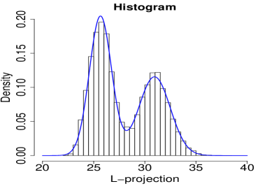
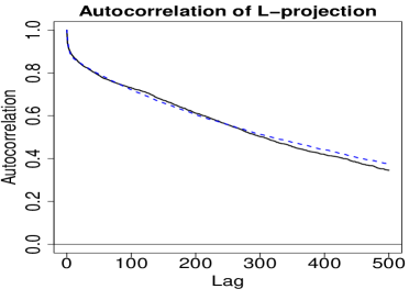
Figure 4: Fit of the diffusion with error model (13) to the sample histogram, and sample autocorrelation function of 20.000 observations of the $L$-reaction coordinate of the small Trp-zipper protein.

Figure 4 shows the fit of the pseudo-likelihood function for the marginal bimodal normal mixture distribution together with the least squares fit of the autocorrelation function (based on the first 100 lags). The parameter estimates are:

$$\hat{\alpha}=0.55,\quad\hat{\mu}_{1}=25.66,\quad\hat{\mu}_{2}=30.94, \hat{\sigma}_{1}=0.54,\quad\hat{\sigma}_{2}=1.22,\quad\hat{\nu}=0.0015,$$

$$\hat{\gamma}^{2}=0.88,\quad \quad\hat{\kappa}=0.43.$$ and

The upper and lower mode of the latent diffusion are estimated by $\hat{u}=\hat{\mu}_{1}$ and $\hat{l}=\hat{\mu}_{2}$, and the implied folding and unfolding rates of the protein given by (9) and (10) are now estimated by:

$$\widehat{E}(T_{\ell}^{Y}|Y_{0}=u) = \frac{\sqrt{2\pi}}{\hat{\nu}}\int_{\widehat{\operatorname{\tau}^{-1}\mu_{1}}}^{\widehat{\operatorname{\tau}^{-1}\mu_{2}}}\{1-\Phi(x)\}e^{x^{2}/2}dx=1138,$$

$$\widehat{E}(T_{u}^{Y}|Y_{0}=\ell) = \frac{\sqrt{2\pi}}{\hat{\nu}}\int_{\widehat{\operatorname{\tau}^{-1}\mu_{1}}}^{\widehat{\operatorname{\tau}^{-1}\mu_{2}}}\Phi(x)e^{x^{2}/2}dx=1320.$$

Folding and unfolding should thus occur on average once in just over a micro second. These estimates are realistic for the protein folding in contrary to the ones implied by the plain diffusion model without measurement error.

As an informal goodness of fit test, we have simulated two trajectories from the plain diffusion model and the diffusion plus noise model, respectively, with parameters equal to those estimated for the data. The simulated data are shown in Figure 5. It is obvious that the model with local error mimics the dynamics of the protein data much better than the plain bimodal diffusion model (without error) does.

Figure 5: Left panel: A simulated sample path of the bimodal diffusion model (7). Right panel: A simulated sample path of the diffusion plus error model (13). Parameters for the simulations were taken from the fit of the two models to the protein data.

5 Conclusion

Flexible and statistically tractable multi-modal diffusion models have been developed, where the multi-modality is caused by a combination of the effects of an energy landscape and of state-dependent random fluctuations. The new diffusion models were obtained by transformations of simple well-studied diffusion models. The transformed diffusion was shown to inherit many properties of the underlying simple diffusion, including its mixing rates and the distributions of first passage times. The eigenfunctions of the infinitesimal generator transform in a straightforward way. Particularly tractable models are obtained by transformations of the Ornstein-Uhlenbeck model, but also transformations of more general Pearson diffusions give tractable multi-model diffusion models.

Likelihood inference and martingale estimating functions were given and investigated in the case of a discretely observed bimodal diffusion. In particular, the theory of martingale estimating functions for transformed diffusions was generalized to the case of parameter-dependent transformations. An estimation method was presented for the case where the bimodal diffusion is observed with additional correlated measurement error.

The new approach was applied to molecular dynamics data in form of a reaction coordinate of the small Trp-zipper protein, where the stationary distribution has two modes corresponding to a folded and an unfolded state. The folding and unfolding rates were estimated by the mean passage times between the two mode points. The new model provides a better fit to this type of protein folding data than previous models because the diffusion coefficient is state-dependent, but the fit is far from perfect. A much more satisfactory fit and realistic folding rates were obtained by adding correlated measurement error reflecting local features of the folding funnel of the protein.

References

- Aït-Sahalia (1996 Aït-Sahalia, Y. (1996). “Testing Continuous-Time Models of the Spot Interest Rate”. The Review of Financial Studies, 9:385–426.
- Aït-Sahalia (2002 Aït-Sahalia, Y. (2002). “Maximum Likelihood Estimation of Discretely Sampled Diffusions: A Closed-Form Approximation Approach”. Econometrica, 70:223–262.
- Ait-Sahalia, Fan & Jiang (2010 Ait-Sahalia, Y.; Fan, J. & Jiang, J. (2010). “Nonparametric tests of the Markov hypothesis in continuous-time models”. Annals of Statististics, 38:3129–3163.
- Alili, Patie & Pedersen (2004 Alili, L.; Patie, P. & Pedersen, J. (2004). “Representations of the First Hitting Time Density of an Ornstein-Uhlenbeck Process”. Stochastic Models, 21:967–980.
- Baltazar-Larios & Sørensen (2010 Baltazar-Larios, F. & Sørensen, M. (2010). “Maximum likelihood estimation for integrated diffusion processes”. In Chiarella, C. & Novikov, A., editors, Contemporary Quantitative Finance: Essays in Honour of Eckhard Platen, pages 407–423. Springer.
- Best & Hummer (2010 Best, R. B. & Hummer, G. (2010). “Coordinate-dependent diffusion in protein folding”. PNAS, 107:1088–1093.
- Bibby, Jacobsen & Sørensen (2010 Bibby, B. M.; Jacobsen, M. & Sørensen, M. (2010). “Estimating Functions for Discretely Sampled Diffusion-type Models”. In Ait-Sahalia, Y. & Hansen, L. P., editors, Handbook of Financial Econometrics, pages 203–268. North-Holland, Oxford.
- Bibby & Sørensen (1997 Bibby, B. M. & Sørensen, M. (1997). “A Hyperbolic Diffusion Model for Stock Prices”. Finance and Stochastics, 1:25–41.
- Bibby & Sørensen (1995 Bibby, B. M. & Sørensen, M. (1995). “Martingale Estimation Functions for Discretely Observed Diffusion Processes”. Bernoulli, 1:17–39.
- Boomsma et al. (2013 Boomsma, W.; Other, A.; Noname, N.; Noname, N. & Noname, N. (2013). “PHAISTOS: A Framework for Markov Chain Monte Carlo Simulation and Inference of Protein Structure”. Forthcoming, Journal of Computational Chemistry.
- Bottaro et al. (2012 Bottaro, S.; Boomsma, W. E.; Johansson, K.; Andreetta, C.; Hamelryck, T. & Ferkinghoff-Borg, J. (2012). “Subtle Monte Carlo updates in dense molecular systems”. Journal of Chemical Theory and Computation, 8:695–702.
- Chahine et al. (2007 Chahine, J.; Oliviera, R. J.; Leite, V. B. P. & Wang, J. (2007). “Configuration-Dependent Diffusion Can Shift the Kinetic Transition State and Barrier Height of Protein Folding”. PNAS, 104:14646–14651.
- Chib, Pitt & Shephard (2006 Chib, S.; Pitt, M. K. & Shephard, N. (2006). “Likelihood based inference for diffusion driven state space models”. Por Clasificar, pages 1–33. http://citeseerx.ist.psu.edu/viewdoc/download?doi=10.1.1.125.5536.
- Das et al. (2006 Das, P.; Moll, M.; Stamati, H.; Kavraki, L. E. & Clementi, C. (2006). “Low-dimensional, free-energy landscapes of protein-folding reactions by nonlinear dimensionality reduction”. PNAS, 103:9885–9890.
- Doukhan (1994 Doukhan, P. (1994). Mixing. Springer-Verlag.
- Fan & Zhang (2003 Fan, J. & Zhang, C. (2003). “A Reexamination of Diffusion Estimators With Applications to Financial Model Validation”. Journal of the American Statistical Association, 98:118–134.
- Forman (2012 Forman, J. L. (2012). “Fully nonparametric bootstrapping of a diffusion process with application to testing the Markov hypothesis”. working paper, Department of Biostatistics, University of Copenhagen.
- Forman & Sørensen (2008 Forman, J. L. & Sørensen, M. (2008). “The Pearson Diffusions: A class of Statistically Tractable Diffusion Processes”. Scandinavian Journal of Statistics, 35:438–465.
- Godambe & Heyde (1987 Godambe, V. P. & Heyde, C. C. (1987). “Quasi likelihood and optimal estimation”. International Statistical Review, 55:231–244.
- Iacus (2008 Iacus, S. M. (2008). Simulatio and Inference for Stochastic Differential Equationsrest Rates. Springer.
- Imkeller & Pavlyukevich (2002 Imkeller, P. & Pavlyukevich, I. (2002). “Model reduction and stochastic resonance”. Stochastics and Dynamics, 2:463–506.
- Jensen & Poulsen (2002 Jensen, B. & Poulsen, R. (2002). “Transition densities of diffusion processes: Numerical comparison of approximation techniques”. Journal of Derivatives, 9:18–32.
- Karlin & Taylor (1981 Karlin, S. & Taylor, H. M. (1981). A Second Course in Stochastic Processes. Academic Press.
- Kessler & Sørensen (1999 Kessler, M. & Sørensen, M. (1999). “Estimating equations based on eigenfunctions for a discretely observed diffusion”. Bernoulli, 5:299–314.
- Lange & Rahbek (2009 Lange, T. & Rahbek, A. (2009). “An Introduction to Regime Switching Time Series Models”. In Andersen, T.; Davis, R.; Kreiss, J. & Mikosch, T., editors, Handbook of Financial Time Series, pages 871–888. Springer.
- Larsen & Sørensen (2007 Larsen, K. S. & Sørensen, M. (2007). “A diffusion model for exchange rates in a target zone”. Mathematical Finance, 17:285–306.
- Pokern, Stuart & Wiberg (2009 Pokern, Y.; Stuart, A. M. & Wiberg, P. (2009). “Parameter estimation for partially observed hypoelliptic diffusions”. J. Roy. Statist. Soc. B, 71:49–73.
- Prinz et al. (2011 Prinz, J.-H.; Wu, H.; Sarich, M.; Keller, B.; Senna, M.; Held, M.; Chodera, J. D.; Schũtte, C. & Noè, F. (2011). “Markov models of molecular kinetics: Generation and validation”. J. Chem. Phys., 134:174105.
- Sørensen (2000 Sørensen, M. (2000). “Prediction-Based Estimating Functions”. Econometrics Journal, 3:123–147.
- Sørensen (2011 Sørensen, M. (2011). “Prediction-based estimating functions: review and new developments”. Brazilian Journal of Probability and Statistics, 25:362–391.
- Sørensen (2012a Sørensen, M. (2012a). “Efficient martingale estimating functions for discretely sampled diffusions”. Preprint.
- Sørensen (2012b Sørensen, M. (2012b). “Estimating functions for diffusion-type processes”. In Kessler, M.; Lindner, A. & Sørensen, M., editors, Statistical Methods for Stochastic Differential Equations, pages 1–107. Chapmann and Hall.
- Socci, Onuchic & Wolynes (1996 Socci, N. D.; Onuchic, J. N. & Wolynes, P. G. (1996). “Diffusive dynamics of the reaction coordinate for protein folding funnels”. J. Chem. Phys., 104:5860–5868.
- Wong (1964 Wong, E. (1964). “The Construction of a Class of Stationary Markoff Processes”. In Bellman, R., editor, Stochastic Processes in Mathematical Physics and Engineering, pages 264–276. American Mathematical Society, Rhode Island.