Average Case and Distributional Analysis of Dual-Pivot Quicksort

Abstract

In 2009, Oracle replaced the long-serving sorting algorithm in its Java 7 runtime library by a new dual-pivot Quicksort variant due to Vladimir Yaroslavskiy. The decision was based on the strikingly good performance of Yaroslavskiy’s implementation in running time experiments. At that time, no precise investigations of the algorithm were available to explain its superior performance — on the contrary: Previous theoretical studies of other dual-pivot Quicksort variants even discouraged the use of two pivots. Only in 2012, two of the authors gave an average case analysis of a simplified version of Yaroslavskiy’s algorithm, proving that savings in the number of comparisons are possible. However, Yaroslavskiy’s algorithm needs more swaps, which renders the analysis inconclusive.

To force the issue, we herein extend our analysis to the fully detailed style of Knuth: We determine the exact number of executed Java Bytecode instructions. Surprisingly, Yaroslavskiy’s algorithm needs sightly more Bytecode instructions than a simple implementation of classic Quicksort — contradicting observed running times. Like in Oracle’s library implementation we incorporate the use of Insertionsort on small subproblems and show that it indeed speeds up Yaroslavskiy’s Quicksort in terms of Bytecodes; but even with optimal Insertionsort thresholds the new Quicksort variant needs slightly more Bytecode instructions on average.

Finally, we show that the (suitably normalized) costs of Yaroslavskiy’s algorithm converge to a random variable whose distribution is characterized by a fixed-point equation. From that, we compute variances of costs and show that for large $n$, costs are concentrated around their mean.

1 Introduction

Quicksort is a divide and conquer sorting algorithm originally proposed by Hoare [1961b; 1961a]. The procedure starts by selecting an arbitrary element from the list to be sorted as pivot. Then, Quicksort partitions the elements into two groups: those smaller than the pivot and those larger than the pivot. After partitioning, we know the exact rank of the pivot element in the sorted list, so we can put it at its final landing position between the groups of smaller and larger elements. Afterwards, Quicksort proceeds by recursively sorting the two parts, until it reaches lists of length zero or one, which are already sorted by definition.

We will in the following always assume random access to the data, i. e., the elements are given as entries of an array. Then, the partitioning process can work in place by directly manipulating the array. This makes Quicksort convenient to use and avoids the need for extra space (except for the recursion stack). Hoare’s initial implementation [Hoare, 1961b] works in place and Sedgewick [1975] studies several variants thereof.

In the worst case, Quicksort has quadratic complexity, namely if in every partitioning step, the pivot is the smallest or largest element of the current subarray. However, this behavior occurs very infrequently, such that the expected complexity is $\Theta(n\log n)$. Hoare [1962] already gives a precise average case analysis of his algorithm, which is nowadays contained in most algorithms textbooks, [e. g. Cormen et al. 2009]. Sedgewick [1975; 1977] refines this analysis to count the exact number of executed primitive instructions of a low level implementation. This detailed breakdown reveals that Quicksort has the asymptotically fastest average running time on MIX among all the sorting algorithm studied by Knuth [1998].

Only considering average results can be misleading. To increase our confidence in a sorting method, we also require that it is likely to observe costs close to the expectation. The standard deviation of the Quicksort complexity grows linearly with $n$ [Knuth, 1998; Hennequin, 1989], which implies that the costs are concentrated around their mean for large $n$. Precise tail bounds which ensure tight concentration around the mean were derived by McDiarmid and Hayward [1996]; see also Fill and Janson [2002].

Much more information is available on the full distribution of the number of key comparisons. When suitably normalized, the number of comparisons converges in law [Regnier, 1989], with a certain unknown limit distribution. Hennequin [1989] computed its first cumulants and proved that it is not a normal distribution. The limiting distribution can be implicitly characterized by a stochastic fixed-point equation [Rösler, 1991] and it is known to have a smooth density [Tan and Hadjicostas, 1995; Fill and Janson, 2000].

Due to its efficiency in the average, Quicksort has been used as general purpose sorting method for decades, for example in the C/C++ standard library and the Java runtime library. As sorting is a widely used elementary task, even small speedups of such library implementations can be worthwhile. This caused a run on variations and modifications to the basic algorithm. One very successful optimization is based on the observation that Quicksort’s performance on tiny subarrays is comparatively poor. Therefore, we should switch to some special purpose sorting method for these cases [Hoare, 1962]. Singleton [1969] proposed using Insertionsort for this task, which indeed “for small $n$ [ …] is about the best sorting method known” according to Sedgewick [1975, p. 22]. He also gives a precise analysis of Quicksort where Insertionsort is used for subproblems of size less than $M$ [Sedgewick, 1977]. For his MIX implementation, the optimal choice is $M=9$, which leads to a speedup of 14 % for $n=10\,000$.

Another very successful optimization is to improve the choice of the pivot element by selecting the median of a small sample of the current subarray. This idea has been studied extensively [Hoare, 1962; Singleton, 1969; Emden, 1970; Sedgewick, 1977; Hennequin, 1989; Chern and Hwang, 2001; Martínez and Roura, 2001; Durand, 2003], and real world implementations make heavy use of it [Bentley and McIlroy, 1993].

Precise analysis of the impact of a modification often helped in understanding and assessing its usefulness, and in fact, many proposed variations turned out detrimental in the end (many examples are exposed by Sedgewick [1975]). Partitioning with more than one pivot used to be counted among those. Sedgewick [1975, p. 150ff] studies a dual-pivot Quicksort variant in detail, but finds that it uses more swaps and comparisons than classic Quicksort. Later Hennequin [1991] considers the general case of partitioning into $s\geq 2$ partitions. For $s=3$, his Quicksort uses asymptotically the same number of comparisons as classic Quicksort; for $s>3$, he attests minor savings which, however, will not compensate for the much more complicated partitioning process in practice. These negative results may have discouraged further research along these lines in the following two decades.

In 2009, however, Vladimir Yaroslavskiy presented his new dual-pivot Quicksort variant at the Java core library mailing list. After promising running time benchmarks, Oracle decided to use Yaroslavskiy’s algorithm as default sorting method for arrays of primitive types in the Java 7 runtime library, even though literature did not offer an explanation for the algorithm’s good performance.

Only in 2012, Wild and Nebel [2012] made a first step towards closing this gap by giving exact expected numbers of swaps and comparisons for a simple version of Yaroslavskiy’s algorithm. We will re-derive these results here as a special case.

The surprising finding is that Yaroslavskiy’s algorithm uses only $1.9n\ln n+\mathrm{O}(n)$ comparisons on average — asymptotically 5 % less than the $2n\ln n+\mathrm{O}(n)$ comparisons needed by classic Quicksort.

The reason for the savings lies in the clever usage of stochastic dependencies: Yaroslavskiy’s algorithm contains two opposite pairs of locations $\mbox{\raisebox{-0.2pt}{\scalebox{1.25}[1.15]{$\mathtt{C}$}}}_{k}$ (lines 1 and 1 of Algorithm 1) and $\mbox{\raisebox{-0.2pt}{\scalebox{1.25}[1.15]{$\mathtt{C}$}}}{}_{\!\mskip 1.0mug}$ (lines 1 and 1) in the code where key comparisons are done: At $\mbox{\raisebox{-0.2pt}{\scalebox{1.25}[1.15]{$\mathtt{C}$}}}_{k}$, elements are first compared with the small pivot $p$ (in line 1) and then with the large pivot $q$ (in line 1) — if still needed, i. e., only if the element is larger than $p$. This means that we need only one comparison to identify a small element, whereas all other elements cost us a second comparisons. For $\mbox{\raisebox{-0.2pt}{\scalebox{1.25}[1.15]{$\mathtt{C}$}}}{}_{\!\mskip 1.0mug}$ it is vice versa: We first compare with $q$, and thus large elements are cheap to identify there.

By the way partitioning is organized, it happens that elements which are initially to the right of the final position of $q$ are classified at $\mbox{\raisebox{-0.2pt}{\scalebox{1.25}[1.15]{$\mathtt{C}$}}}{}_{\!\mskip 1.0mug}$; whereas elements to the left are classified at $\mbox{\raisebox{-0.2pt}{\scalebox{1.25}[1.15]{$\mathtt{C}$}}}_{k}$. This implies that the number of elements classified at $\mbox{\raisebox{-0.2pt}{\scalebox{1.25}[1.15]{$\mathtt{C}$}}}{}_{\!\mskip 1.0mug}$ co-varies with the number of large elements: $\mbox{\raisebox{-0.2pt}{\scalebox{1.25}[1.15]{$\mathtt{C}$}}}{}_{\!\mskip 1.0mug}$ is executed more often if there are more elements larger than $q$ (on average) and similarly, $\mbox{\raisebox{-0.2pt}{\scalebox{1.25}[1.15]{$\mathtt{C}$}}}_{k}$ is visited often if there are many small elements. Consequently, the probability that one comparison suffices to determine an element’s target partition is strictly larger than $1\mskip 1.0mu/\mskip 1.0mu3$ — which would be the probability if all elements are first compared to $p$ (or all first to $q$). The asymmetric treatment of elements is the novelty that makes Yaroslavskiy’s algorithm superior to the dual-pivot partitioning schemes studied earlier.

While the lower number of comparisons seems promising, Yaroslavskiy’s dual-pivot Quicksort needs more swaps than classic Quicksort, so the high level analysis remains inconclusive. In this paper, we extend our analysis to detailed instruction counts, complementing previous work on classic Quicksort [Sedgewick, 1977]. However, instead of Knuth’s slightly dated mythical machine MIX, we consider the Java Virtual Machine [Lindholm and Yellin, 1999] and count the number of executed Java Bytecode instructions. Wild [2012] gives similar results for Knuth’s MMIX [Knuth, 2005], the successor of MIX.

The number of executed Bytecode instructions has been shown to resemble actual running time [Camesi et al., 2006], even though just-in-time compilation can have a tremendous influence [Wild et al., 2013] and some aspects of modern processor architectures are neglected.

Extending the results of Wild and Nebel [2012], the analysis in this paper includes sorting short subproblems with Insertionsort. Moreover, all previous results on Yaroslavskiy’s algorithm only concern expected behavior. In this article, we show existence and give characterizations of limit distributions. A comforting result of these studies is that the standard deviation grows linearly for Yaroslavskiy’s algorithm as well, which implies concentration around the mean.

This paper does not consider more refined ways to choose pivots, like selecting order statistics of a random sample. We decided to defer a detailed treatment of Yaroslavskiy’s algorithm under this optimization to a separate article [Nebel and Wild, 2014].

The rest of this paper is organized as follows. Section 1.1 presents our object of study. In Section 2, we review basic notions used in the analysis later. We also define our input model and collect elementary properties of Yaroslavskiy’s algorithm. In Section 3, we derive exact average costs in terms of comparisons, swaps and executed Bytecode instructions. These are used in Section 4 to identify a limiting distribution of normalized costs in all three measures, from which we obtain asymptotic variances. Finally, Section 5 summarizes our findings and puts them in context.

1.1 Yaroslavskiy’s Algorithm

• $\textnormal{QuicksortYaroslavskiy}\,(\smash{\raisebox{-0.2pt}{\scalebox{1.25}[1.18]{$\mathtt{A}$}}},\mathit{left},\mathit{right})$
       // Sort $\smash{\raisebox{-0.2pt}{\scalebox{1.25}[1.18]{$\mathtt{A}$}}}[\mathit{left},\dots,\mathit{right}]$ (including end points). $1$if $\mathit{right}-\mathit{left}<M$     // i. e. the subarray has $n\leq M$ elements $2$ InsertionSort$(\smash{\raisebox{-0.2pt}{\scalebox{1.25}[1.18]{$\mathtt{A}$}}},\mathit{left},\mathit{right})$ $3$else $4$ if $\smash{\raisebox{-0.2pt}{\scalebox{1.25}[1.18]{$\mathtt{A}$}}}[\mathit{left}]>\smash{\raisebox{-0.2pt}{\scalebox{1.25}[1.18]{$\mathtt{A}$}}}[\mathit{right}]$ $5$ $p\mathrel{\hskip 1.0pt:=\hskip 1.0pt}\smash{\raisebox{-0.2pt}{\scalebox{1.25}[1.18]{$\mathtt{A}$}}}[\mathit{right}]$; $q\mathrel{\hskip 1.0pt:=\hskip 1.0pt}\smash{\raisebox{-0.2pt}{\scalebox{1.25}[1.18]{$\mathtt{A}$}}}[\mathit{left}]$ $6$ else $7$ $p\mathrel{\hskip 1.0pt:=\hskip 1.0pt}\smash{\raisebox{-0.2pt}{\scalebox{1.25}[1.18]{$\mathtt{A}$}}}[\mathit{left}]$; $q\mathrel{\hskip 1.0pt:=\hskip 1.0pt}\smash{\raisebox{-0.2pt}{\scalebox{1.25}[1.18]{$\mathtt{A}$}}}[\mathit{right}]$ $8$ end if $9$ $\ell\mathrel{\hskip 1.0pt:=\hskip 1.0pt}\mathit{left}+1$;  $g\mathrel{\hskip 1.0pt:=\hskip 1.0pt}\mathit{right}-1$;  $k\mathrel{\hskip 1.0pt:=\hskip 1.0pt}\ell$ $10$ while $k\leq g$ $11$ if $\smash{\raisebox{-0.2pt}{\scalebox{1.25}[1.18]{$\mathtt{A}$}}}[k]<p$ $12$ Swap $\smash{\raisebox{-0.2pt}{\scalebox{1.25}[1.18]{$\mathtt{A}$}}}[k]$ and $\smash{\raisebox{-0.2pt}{\scalebox{1.25}[1.18]{$\mathtt{A}$}}}[\ell]$ $13$ $\ell\mathrel{\hskip 1.0pt:=\hskip 1.0pt}\ell+1$ $14$ else $15$ if $\smash{\raisebox{-0.2pt}{\scalebox{1.25}[1.18]{$\mathtt{A}$}}}[k]\geq q$ $16$ while $\smash{\raisebox{-0.2pt}{\scalebox{1.25}[1.18]{$\mathtt{A}$}}}[g]>q$ and $k<g$ do $g\mathrel{\hskip 1.0pt:=\hskip 1.0pt}g-1$ end while $17$ if $\smash{\raisebox{-0.2pt}{\scalebox{1.25}[1.18]{$\mathtt{A}$}}}[g]\geq p$ $18$ Swap $\smash{\raisebox{-0.2pt}{\scalebox{1.25}[1.18]{$\mathtt{A}$}}}[k]$ and $\smash{\raisebox{-0.2pt}{\scalebox{1.25}[1.18]{$\mathtt{A}$}}}[g]$ $19$ else $20$ Swap $\smash{\raisebox{-0.2pt}{\scalebox{1.25}[1.18]{$\mathtt{A}$}}}[k]$ and $\smash{\raisebox{-0.2pt}{\scalebox{1.25}[1.18]{$\mathtt{A}$}}}[g]$;   Swap $\smash{\raisebox{-0.2pt}{\scalebox{1.25}[1.18]{$\mathtt{A}$}}}[k]$ and $\smash{\raisebox{-0.2pt}{\scalebox{1.25}[1.18]{$\mathtt{A}$}}}[\ell]$ $21$ $\ell\mathrel{\hskip 1.0pt:=\hskip 1.0pt}\ell+1$ $22$ end if $23$ $g\mathrel{\hskip 1.0pt:=\hskip 1.0pt}g-1$ $24$ end if $25$ end if $26$ $k\mathrel{\hskip 1.0pt:=\hskip 1.0pt}k+1$ $27$ end while $28$ $\ell\mathrel{\hskip 1.0pt:=\hskip 1.0pt}\ell-1$; $g\mathrel{\hskip 1.0pt:=\hskip 1.0pt}g+1$ $29$ $\smash{\raisebox{-0.2pt}{\scalebox{1.25}[1.18]{$\mathtt{A}$}}}[\mathit{left}]\mathrel{\hskip 1.0pt:=\hskip 1.0pt}\smash{\raisebox{-0.2pt}{\scalebox{1.25}[1.18]{$\mathtt{A}$}}}[\ell]$; $\smash{\raisebox{-0.2pt}{\scalebox{1.25}[1.18]{$\mathtt{A}$}}}[\ell]\mathrel{\hskip 1.0pt:=\hskip 1.0pt}p$   // Swap pivots to final position $30$ $\smash{\raisebox{-0.2pt}{\scalebox{1.25}[1.18]{$\mathtt{A}$}}}[\mathit{right}]\mathrel{\hskip 1.0pt:=\hskip 1.0pt}\smash{\raisebox{-0.2pt}{\scalebox{1.25}[1.18]{$\mathtt{A}$}}}[g]$; $\smash{\raisebox{-0.2pt}{\scalebox{1.25}[1.18]{$\mathtt{A}$}}}[g]\mathrel{\hskip 1.0pt:=\hskip 1.0pt}q$ $31$ $\textnormal{QuicksortYaroslavskiy}\,(\smash{\raisebox{-0.2pt}{\scalebox{1.25}[1.18]{$\mathtt{A}$}}},\hbox{\makebox[20.11565pt][c]{\makebox[0.0pt][c]{$\mathit{left}$}}},\hbox{\makebox[20.11565pt][c]{\makebox[0.0pt][c]{$\ell-1$}}})$ $32$ $\textnormal{QuicksortYaroslavskiy}\,(\smash{\raisebox{-0.2pt}{\scalebox{1.25}[1.18]{$\mathtt{A}$}}},\hbox{\makebox[20.11565pt][c]{\makebox[0.0pt][c]{$\ell+1$}}},\hbox{\makebox[20.11565pt][c]{\makebox[0.0pt][c]{$g-1$}}})$ $33$ $\textnormal{QuicksortYaroslavskiy}\,(\smash{\raisebox{-0.2pt}{\scalebox{1.25}[1.18]{$\mathtt{A}$}}},\hbox{\makebox[20.11565pt][c]{\makebox[0.0pt][c]{$g+1$}}},\hbox{\makebox[20.11565pt][c]{\makebox[0.0pt][c]{$\mathit{right}$}}})$ $34$end if

Algorithm 1 Yaroslavskiy’s Dual-Pivot Quicksort with Insertionsort.

Yaroslavskiy’s dual-pivot Quicksort is shown in Algorithm 1. The initial call to the procedure takes the form QuicksortYaroslavskiy$(\smash{\raisebox{-0.2pt}{\scalebox{1.25}[1.18]{$\mathtt{A}$}}},1,n)$, where $\mathtt{A}$ is an array containing the elements to be sorted and $n$ is its length. After selecting the outermost elements as pivots $p$ and $q$ such that $p\leq q$, lines 1 – 1 of Algorithm 1 comprise the partitioning method. After that, all small elements, i. e., those smaller than $p$ (and $q$), form a contiguous region at the left end of the array, followed by $p$ and the medium elements. Finally $q$ separates the medium and large elements. After recursively sorting these three regions, the whole array is in order.

Yaroslavskiy’s partitioning algorithm is an asymmetric generalization of Hoare’s crossing pointers technique: The index pointers $k$ and $g$ start at the left and right ends, respectively, and are moved towards each other until they cross. Additionally, pointer $\ell$ marks the position of the rightmost small element, such that the array is kept invariably in the following form:

Our Algorithm 1 differs from Algorithm 3 of [Wild and Nebel, 2012] as follows:

• For lists of length less than $M$, we switch to InsertionSort. A possible implementation is given in Appendix B. The case $M=1$ corresponds to not using Insertionsort at all.

• The swap of $\smash{\raisebox{-0.2pt}{\scalebox{1.25}[1.18]{$\mathtt{A}$}}}[k]$ and $\smash{\raisebox{-0.2pt}{\scalebox{1.25}[1.18]{$\mathtt{A}$}}}[g]$ has been moved behind the check $\smash{\raisebox{-0.2pt}{\scalebox{1.25}[1.18]{$\mathtt{A}$}}}[g]\geq p$. Thereby, we never use array positions in a key comparison after we have overwritten their contents in one partitioning step; see Fact 2.3 below. (This is just to simplify discussions.)

• The comparison in line 1 has been made non-strict. For distinct elements this makes no difference, but it drastically improves performance in case of many equal keys [Wild, 2012, p. 54]. The reader might find it instructive to consider the behavior on an array with all elements equal.

Note that partitioning an array around two pivots is similar in nature to the Dutch National Flag Problem (DNFP) posed by Dijkstra [1976] as a programming exercise:

Given an array of $n$ red, white and blue pebbles, rearrange them by swaps, such that the colors form the Dutch national flag: red, white and blue in contiguous regions. Each pebble may be inspected only once and only a constant amount of extra storage may be used.

Dijkstra assumes an operation “buck” that tells us an element’s color in one shot, so any algorithm must use exactly $n$ buck-operations. Performance differences only concern the number of swaps needed.

Interestingly, Meyer gave an algorithm for the DNFP which is essentially equivalent to Yaroslavskiy’s partitioning method. Indeed, it even outperforms the algorithm proposed by Dijkstra [McMaster, 1978]! Yet, the real advantage of Yaroslavskiy’s partitioning scheme — the reduced expected number of key comparisons — is hidden by the atomic buck operation; its potential use in Quicksort went unnoticed.

2 Preliminaries

In this section, we recall elementary definitions and collect some notation and basic facts used throughout this paper.

By $\mathcal{H}_{n}\colonequals\sum_{i=1}^{n}1\mathbin{/}i$, we denote the $n$th Harmonic Number. We use $\delta_{i\!j}$ for the Kronecker delta, which is defined to be $1$ if $i=j$ and $0$ otherwise. We define $x\ln(x)=0$ for $x=0$, so that $x\mapsto x\ln(x)$ becomes a continuous function on $[0,\infty)$.

The probability of an event $E$ is denoted by $\mathbb{P}[E]$ and we write $\mathbb{1}_{\{E\}}$ for its indicator random variable, which is $1$ if the event occurs and $0$ otherwise. For a random variable $X$, let $\mathop{\mbox{$\mathbb{E}$}}\nolimits[X]$, $\mathrm{Var}(X)$ and ${\cal L}(X)$ denote its expectation, variance and distribution, respectively. $X\mathrel{\smash{\mathchoice{\mathrel{\overset{\raisebox{0.0pt}{$\scriptstyle\cal D$}}{=}}}{\mathrel{\hbox{\makebox[7.7778pt][c]{\makebox[0.0pt][c]{$\overset{\raisebox{-4.30554pt}{$\scriptscriptstyle\cal D$}}{=}$}}}}}{\mathrel{\overset{\cal D}{=}}}{\mathrel{\overset{\cal D}{=}}}}}Y$ means that $X$ has the same distribution as $Y$.

By $\|X\|_{p}\colonequals\mathop{\mbox{$\mathbb{E}$}}\nolimits[|X|^{p}]^{1/p}$, $1\leq p<\infty$, we denote the $L_{p}$-norm of random variable $X$. For random variables $X_{1},X_{2},\ldots$ and $X$, we say $X_{n}$ converges in $L_{p}$ to $X$

$$X_{n}\mathrel{\;\;{\overset{L_{p}}{\longrightarrow}}\;\;}X\qquad\qquad\text{iff}\qquad\qquad\lim_{n\to\infty}\|X_{n}-X\|_{p}\mathrel{\;\;{=}\;\;}0\;.$$

The Bernoulli distribution with parameter $p$ is written as $\mathrm{B}(p)$. Provided that $\sum_{r=1}^{b}p_{r}=1$ and $b\geq 1$ is a fixed integer, we denote by $\mathrm{M}(n;p_{1},\ldots,p_{b})$ the multinomial distribution with $n$ trials and success probabilities $p_{1},\ldots,p_{b}\in[\mskip 1.0mu0,1]$. For random probabilities $V=(V_{1},\ldots,V_{b})$, i. e., random variables $0\leq V_{r}\leq 1$ ($r=1,\ldots,b$) with $\sum_{r=1}^{b}V_{r}=1$ almost surely, we write $Y\mathchoice{\mathrel{\overset{\raisebox{0.0pt}{$\scriptstyle\cal D$}}{=}}}{\mathrel{\hbox{\makebox[7.7778pt][c]{\makebox[0.0pt][c]{$\overset{\raisebox{-4.30554pt}{$\scriptscriptstyle\cal D$}}{=}$}}}}}{\mathrel{\overset{\cal D}{=}}}{\mathrel{\overset{\cal D}{=}}}\mathrm{M}(n;V_{1},\ldots,V_{b})$ to denote that $Y$ conditional on $V=v$ (i. e., conditional on $(V_{1},\ldots,V_{b})=(v_{1},\ldots,v_{b})$) is multinomially $\mathrm{M}(n;v_{1},\ldots,v_{b})$ distributed.

For $k,r,b\in\mathbb{N}$ satisfying $k\leq r+b$, the hypergeometric distribution with $k$ trials from $r$ red and $b$ black balls is denoted by $\mathrm{HypG}(k,r,r+b)$. Given an urn with $r$ red and $b$ black balls, it is the distribution of the number of red balls drawn when drawing $k$ times without replacement. The mean and variance of a hypergeometrically $\mathrm{HypG}(k,r,r+b)$ distributed random variable $G$ are given by [Kendall, 1945, p. 127]

$$\mathop{\mbox{$\mathbb{E}$}}\nolimits[G] \mathrel{\;\;{=}\;\;}k\cdot\frac{r}{r+b}\,, \mathrm{Var}(G) \mathrel{\;\;{=}\;\;}\frac{krb(r+b-k)}{(r+b)^{2}(r+b-1)}\;.$$ (2.1)

As for the multinomial distribution, given random parameters $K$, $R$ in $\{0,\ldots,n\}$ we use $Y\mathchoice{\mathrel{\overset{\raisebox{0.0pt}{$\scriptstyle\cal D$}}{=}}}{\mathrel{\hbox{\makebox[7.7778pt][c]{\makebox[0.0pt][c]{$\overset{\raisebox{-4.30554pt}{$\scriptscriptstyle\cal D$}}{=}$}}}}}{\mathrel{\overset{\cal D}{=}}}{\mathrel{\overset{\cal D}{=}}}\mathrm{HypG}(K,R,n)$ to denote that $Y$ conditional on $(K,R)=(k,r)$ is hypergeometrically $\mathrm{HypG}(k,r,n)$ distributed.

2.1 Input Model

We assume the random permutation model: The keys to be sorted are the integers $1,\ldots,n$ and each permutation of $\{1,\dots,n\}$ has equal probability $1\mskip 1.0mu/n!$ to become the input. Note that we implicitly exclude the case of equal keys by that.

As sorting is only concerned with the relative order of elements, not the key values themselves, we can equivalently assume keys to be i. i. d. real random variables from any (non-degenerate) continuous distribution. Equal keys do not occur almost surely and the ranks of the elements form in fact a random permutation of $\{1,\dots,n\}$ again [see e. g. Mahmoud 2000]. For the analysis of Section 4, this alternative point of view will be helpful.

2.2 Basic Properties of Yaroslavskiy’s Algorithm

As typical for divide and conquer algorithms, the analysis is based on setting up a recurrence relation for the costs. For such a recurrence to hold, it is vital that the costs for subproblems of size $k$ behave the same as the costs for dealing with an original random input of initial size $k$. For Quicksort, we require the following property:

Property 2.1 (Randomness Preservation).

If the whole input is a (uniformly chosen) random permutation of its elements, so are the subproblems Quicksort is recursively invoked on.

Hennequin [1989] showed that Property 2.1 is implied by the following property.

Property 2.2 (Sufficient Condition for Randomness Preservation).

Every key comparison involves a pivot element of the current partitioning step.

Now, it is easy to verify that Yaroslavskiy’s algorithm fulfills Property 2.2 and hence Property 2.1.

Since Yaroslavskiy’s algorithm is an in-place sorting method, it modifies the array  $\mathtt{A}$ over time. This dynamic component makes discussions inconvenient. Fortunately, a sharp look at the algorithm reveals the following fact, allowing a more static point of view:

Fact 2.3.

The array elements used in key comparisons have not been changed since the beginning of the current partitioning step. More precisely, if a key comparison involves an array element $\smash{\raisebox{-0.2pt}{\scalebox{1.25}[1.18]{$\mathtt{A}$}}}[i]$, then there has not been a write access to $\smash{\raisebox{-0.2pt}{\scalebox{1.25}[1.18]{$\mathtt{A}$}}}[i]$ in the current partitioning step. ∎

3 Average Case Analysis

Throughout Section 3, we assume that array $\mathtt{A}$ stores a random permutation of $\{1,\ldots,n\}$.

3.1 The Dual-Pivot Quicksort Recurrence

In this section, we obtain a general solution to the recurrence relation corresponding to dual-pivot Quicksort. We denote by $\mathop{\mbox{$\mathbb{E}$}}\nolimits[C_{n}]$ the expected costs — where different cost measures will be inserted later — of Yaroslavskiy’s algorithm on a random permutation of $\{1,\ldots,n\}$. $\mathop{\mbox{$\mathbb{E}$}}\nolimits[C_{n}]$ decomposes as

$$\mathop{\mbox{$\mathbb{E}$}}\nolimits[C_{n}] \mathrel{\;\;{=}\;\;}\text{costs of first partitioning step}\mathbin{\;{+}\;}\text{costs for subproblems}\;.$$ (3.1)

As Yaroslavskiy’s algorithm satisfies Property 2.1, the costs for recursively sorting subarrays can be expressed in terms of $C$ with smaller arguments, leading to a recurrence relation. Every (sorted) pair of elements has the same probability $1\big{/}\binom{n}{2}$ of becoming pivots. Conditioning on the ranks of the pivots, this gives the following recursive form for the expected costs $\mathop{\mbox{$\mathbb{E}$}}\nolimits[C_{n}]$ of Yaroslavskiy’s algorithm on a random permutation of size $n$:

$$\mathop{\mbox{$\mathbb{E}$}}\nolimits[C_{n}] \mathrel{\;{=}\;}\begin{cases}\displaystyle\mathop{\mbox{$\mathbb{E}$}}\nolimits[T\!_{n}]\mathbin{\;{+}\;}1\big{/}\tbinom{n}{2}\!\!\!\sum_{1\leq p<q\leq n}\!\!\!\bigl{(}\mathop{\mbox{$\mathbb{E}$}}\nolimits[C_{p-1}]+\mathop{\mbox{$\mathbb{E}$}}\nolimits[C_{q-p-1}]+\mathop{\mbox{$\mathbb{E}$}}\nolimits[C_{n-q}]\bigr{)}\,,&\text{for }n>M;\\ \mathop{\mbox{$\mathbb{E}$}}\nolimits[C^{\mathrm{IS}}_{n}]\,,&\text{for }n\leq M,\end{cases}$$ (3.2)

where $C^{\mathrm{IS}}_{n}$ denotes the costs of InsertionSorting a random permutation of $\{1,\ldots,n\}$ and $T\!_{n}$ is the cost contribution of the first partitioning step. This function $T\!_{n}$ quantifies the “toll” we have to pay for unfolding the recurrence once, therefore we will call $T\!_{n}$ the toll function of the recurrence. By adapting the toll function, we can use the same recurrence to describe different kinds of costs and we only need to derive a general solution to this single recurrence relation as provided by the following theorem:

Theorem 3.1.

Let $\mathop{\mbox{$\mathbb{E}$}}\nolimits[C_{n}]$ be recursively defined by (3.2). Then, $\mathop{\mbox{$\mathbb{E}$}}\nolimits[C_{n}]$ satisfies

$$\mathop{\mbox{$\mathbb{E}$}}\nolimits[C_{n}]\mathrel{\;\;{=}\;\;}\frac{1}{\tbinom{n}{4}}\sum_{i=M+4}^{n}\!\!\!\tbinom{i}{4}\!\!\!\sum_{j=M+2}^{i-2}\biggl{(}\mathop{\mbox{$\mathbb{E}$}}\nolimits[T\!_{j+2}]\mathbin{\>{-}\>}\tfrac{2j}{j+2}\mathop{\mbox{$\mathbb{E}$}}\nolimits[T\!_{j+1}]\mathbin{\>{+}\>}\tfrac{\tbinom{j}{2}}{\tbinom{j+2}{2}}\mathop{\mbox{$\mathbb{E}$}}\nolimits[T\!_{j}]\biggr{)}\\ \mathbin{\;{+}\;}\biggl{(}\!\tfrac{n+1}{5}+\frac{\tbinom{M+3}{4}-\tbinom{M+4}{5}}{\tbinom{n}{4}}\biggr{)}\mathop{\mbox{$\mathbb{E}$}}\nolimits[C_{M+3}]\mathbin{\;\;{-}\;\;}\tfrac{M-1}{M+3}\biggl{(}\!\tfrac{n+1}{5}-\frac{\tbinom{M+4}{5}}{\tbinom{n}{4}}\biggr{)}\mathop{\mbox{$\mathbb{E}$}}\nolimits[C_{M+2}]\,,\qquad\text{for }n\geq M+3.$$ (3.3)

As an immediate consequence, $\mathop{\mbox{$\mathbb{E}$}}\nolimits[C_{n}]$ — seen as a function of $\mathop{\mbox{$\mathbb{E}$}}\nolimits[T\!_{n}]$ — is linear in $\mathop{\mbox{$\mathbb{E}$}}\nolimits[T\!_{n}]$.

The proof for Theorem 3.1 uses several layers of successive differences of $\mathop{\mbox{$\mathbb{E}$}}\nolimits[C_{n}]$ to finally obtain a telescoping recurrence. Substituting back in then yields (3.3). The detailed computations are given in Appendix A. This general solution still involves non-trivial double sums. For the cost measures we are interested in, the following proposition gives an explicit solution for (3.2).

Proposition 3.2.

Let $\mathop{\mbox{$\mathbb{E}$}}\nolimits[C_{n}]$ be recursively defined by (3.2) and let $\mathop{\mbox{$\mathbb{E}$}}\nolimits[T\!_{n}]=an+b$ for $n\geq M+1$. Then, $\mathop{\mbox{$\mathbb{E}$}}\nolimits[C_{n}]$ satisfies

$$\mathop{\mbox{$\mathbb{E}$}}\nolimits[C_{n}]\mathrel{\;\;{=}\;\;}\tfrac{6}{5}a(n+1)\bigl{(}\mathcal{H}_{n+1}-\mathcal{H}_{M+2}\bigr{)}\mathbin{\;{+}\;}\tfrac{1}{5}(n+1)\bigl{(}\tfrac{19}{5}a+\tfrac{6(b-a)}{M+2}\bigr{)}\mathbin{\;{+}\;}\tfrac{a-b}{2}\\ \mathbin{\;{+}\;}\tfrac{1}{5}(n+1)\sum_{k=0}^{M}\frac{3M-2k}{\tbinom{M+2}{3}}\mathop{\mbox{$\mathbb{E}$}}\nolimits[C^{\mathrm{IS}}_{k}]\mathbin{\;\;{+}\;\;}\frac{\tbinom{M+4}{5}}{\tbinom{n}{4}}R_{M}\,,\qquad\text{for }n\geq M+3,$$ (3.4)

where

$$R_{M}\mathrel{\;\;{=}\;\;}\tfrac{6}{5}a+\tfrac{2(a-b)}{M+3}+\tfrac{5b-17a}{2(M+4)}-\tfrac{M-1}{M+4}\mathop{\mbox{$\mathbb{E}$}}\nolimits[C_{M+3}]+\tfrac{M-1}{M+3}\mathop{\mbox{$\mathbb{E}$}}\nolimits[C_{M+2}]\;.$$

If $\mathop{\mbox{$\mathbb{E}$}}\nolimits[C^{\mathrm{IS}}_{n}=0]$ for all $n$, $\mathop{\mbox{$\mathbb{E}$}}\nolimits[C_{n}]$ has the following asymptotic representation:

$$\mathop{\mbox{$\mathbb{E}$}}\nolimits[C_{n}] \mathrel{\;\;{=}\;\;}\tfrac{6}{5}an\ln n\mathbin{\;{+}\;}\bigl{(}\tfrac{19}{25}a+W\bigr{)}\mskip 1.0mun\mathbin{\;{+}\;}\tfrac{6}{5}a\ln n\mathbin{\;{+}\;}\bigl{(}\tfrac{153}{50}a-\tfrac{1}{2}b+W\bigr{)}\mathbin{\;\;{+}\;\;}\mathrm{O}\bigl{(}\tfrac{1}{n}\bigr{)}\,,\qquad n\to\infty,$$ (3.5)

where

$$W \mathrel{\;\;{=}\;\;}\tfrac{6}{5}\bigl{(}a\,\gamma+\tfrac{b-a}{M+2}-a\mathcal{H}_{M+2}\bigr{)}$$

and $\gamma\approx 0.57721$ is the Euler-Mascheroni constant.

Moreover, if the toll function $\mathop{\mbox{$\mathbb{E}$}}\nolimits[T\!_{n}]$ has essentially the form given above, but with $\mathop{\mbox{$\mathbb{E}$}}\nolimits[T\!_{2}]=0\neq 2a+b$, we get an additional summand $-\delta_{M1}\cdot\smash{\tfrac{1}{10}}(2a+b)\cdot(n+1)$ in (3.4). Equation (3.5) remains valid if we set $W=\tfrac{6}{5}\bigl{(}a\,\gamma+\tfrac{b-a}{M+2}-a\mathcal{H}_{M+2}-\delta_{M1}(2a+b)\mathbin{/}10\bigr{)}$.

The proof of Proposition 3.2 is basically “by computing”, the details are again deferred to Appendix A.

Remark: For constant $M$, i. e., $M=\Theta(1)$ as $n\to\infty$, only the linear term of the expected costs is affected by $M$. This means that for the leading term of $\mathop{\mbox{$\mathbb{E}$}}\nolimits[C_{n}]$, the “base case strategy” for solving small subproblems is totally irrelevant.

3.2 Basic Block Execution Frequencies

In this section, we compute for every single instruction of Yaroslavskiy’s algorithm how often it is executed in expectation. Based on that, we can easily derive the expected number of key comparisons, swaps, but also more detailed measures, such as the expected number of executed Bytecode instructions. This is the kind of analysis Knuth popularized through his book series The Art of Computer Programming [Knuth, 1998]. A corresponding analysis of classic single pivot Quicksort was done by Sedgewick [1977]. Like the Quicksort variant discussed there, Algorithm 1 uses Insertionsort for sorting small subarrays. Our detailed implementation of Insertionsort and its analysis are given in Appendix B.

Consecutive lines of purely sequential code always have the same execution frequencies; contracting maximal blocks of such code yields the control flow graph (CFG). Figure 1 shows the resulting CFG for Yaroslavskiy’s algorithm. Simple flow conservation arguments (a. k. a. Kirchhoff’s laws) allow to express execution frequencies of some blocks by the frequencies of others: The execution frequencies of the $20$ basic blocks of Figure 1 only depend on the following nine frequencies: $A$, $B$, $R$, $F$, $C^{\smash{(1)}}$, $C^{\smash{(3)}}$, $C^{\smash{(4)}}$, $S^{\smash{(1)}}$ and $S^{\smash{(3)}}$. The name $C^{\smash{(i)}}$ indicates that this frequency counts executions of the $i$th location in the code of Algorithm 1, where a key comparison is done. Similarly, $S^{\smash{(i)}}$ corresponds to the $i$th swap location.

Figure 1: Control flow graph for Algorithm 1. The algorithm is decomposed into basic blocks of purely sequential code. Possible transitions from one block to another are indicated by arrows. Blocks with two outgoing arrows end with a conditional, the “yes” path is taken if the condition is fulfilled, otherwise the “no” transition is chosen. We refer to blocks using the number shown in the upper left corner. In the upper right corner, a block’s symbolic execution frequency is given. For clarity of presentation, the recursive calls in block 1 are not explicitly shown, but only sketched by the dashed arrows. Block 1 calls InsertionSort which is given in Appendix B.

The results are summarized in Tables 1 and 2 at the end of the section.

The expected execution frequencies allow a recursive representation of the following form, here using the example of $C^{\smash{(1)}}$:

$$\mathop{\mbox{$\mathbb{E}$}}\nolimits[C^{\smash{(1)}}_{n}] \mathrel{\;\;{=}\;\;}\begin{cases}\displaystyle\mathop{\mbox{$\mathbb{E}$}}\nolimits[T_{\!C^{\smash{(1)}}}({n})]\displaystyle\mathbin{\;\;{+}\;\;}1\big{/}\tbinom{n}{2}\!\!\!\!\!\!\sum_{1\leq p<q\leq n}\!\!\!\bigl{(}\mathop{\mbox{$\mathbb{E}$}}\nolimits[C^{\smash{(1)}}_{p-1}]+\mathop{\mbox{$\mathbb{E}$}}\nolimits[C^{\smash{(1)}}_{q-p-1}]+\mathop{\mbox{$\mathbb{E}$}}\nolimits[C^{\smash{(1)}}_{n-q}]\bigr{)}\,,&\text{for }n>M;\\ 0,&\text{for }n\leq M,\end{cases}\,,$$ (3.6)

where $T_{\!C^{\smash{(1)}}}=T_{\!C^{\smash{(1)}}}({n})$ is the frequency specific toll function — namely the corresponding frequency during the first partitioning step only. For the other frequencies, we similarly denote by $T_{\!A}$, $T_{\!F}$, $T_{\!C^{\smash{(3)}}}$, $T_{\!C^{\smash{(4)}}}$, $T_{\!S^{\smash{(1)}}}$ and $T_{\!S^{\smash{(3)}}}$ the toll functions corresponding to $A$, $F$, $C^{\smash{(3)}}$, $C^{\smash{(4)}}$, $S^{\smash{(1)}}$ and $S^{\smash{(3)}}$, respectively.

The frequencies $F$, $C^{\smash{(1)}}$, $C^{\smash{(3)}}$, $C^{\smash{(4)}}$, $S^{\smash{(1)}}$ and $S^{\smash{(3)}}$ correspond to basic blocks in the body of the main partitioning loop, i. e., blocks 1 – 1. All these blocks have in common that they are not executed at all during calls with $\mathit{right}-\mathit{left}\leq 1$, i. e., when $n\leq 2$: In that case we have $k>g$ directly after block 1 and hence immediately leave the partitioning loop from block 1 to block 1. Therefore, we have $T_{\!F}({2})=T_{\!C^{\smash{(1)}}}({2})=T_{\!C^{\smash{(3)}}}({2})=T_{\!C^{\smash{(4)}}}({2})=T_{\!S^{\smash{(1)}}}({2})=T_{\!S^{\smash{(3)}}}({2})=0$. In the subsequent sections, we will determine the toll functions for $n\geq 3$.

For that, we will first compute their values given fixed pivot ranks $P$ and $Q$, i. e., we determine their distribution conditional on $(P,Q)=(p,q)$. Here, we capitalized $P$ and $Q$ to emphasize the fact that the pivot ranks are themselves random variables. Then, we get the unconditional expected frequencies via the law of total expectation. Note that for permutations of $\{1,\ldots,n\}$, ranks and values coincide and we will not always dwell on the difference to keep the presentation concise, but unless stated otherwise, $P$ and $Q$ refer to the ranks of the two pivots.

3.2.1 The Crossing Point Lemma

The following lemma is the key to the precise analysis of the execution frequencies that depend on how pointers $k$ and $g$ “cross”. As the pointers are moved alternatingly towards each other, one of them will reach the crossing point first — waiting for the other to arrive.

Lemma 3.3 (Crossing Point Lemma).

Let $\mathtt{A}$ store a random permutation of $\{1,\dots,n\}$ with $n\geq 2$. Then, Algorithm 1 leaves the outer loop of the first partitioning step with

$$k\mathrel{\;\;{=}\;\;}q+\delta\mathrel{\;\;{=}\;\;}g+1+\delta\,,\qquad\text{where }\delta=0\text{ or }\delta=1.$$ (3.7)

(More precisely, (3.7) holds for the valuations of $k$, $g$ and $q$ upon entrance of block 1).
Moreover, $\delta=1$ iff initially $\smash{\raisebox{-0.2pt}{\scalebox{1.25}[1.18]{$\mathtt{A}$}}}[q]>q$ holds, where $q=\max\{\smash{\raisebox{-0.2pt}{\scalebox{1.25}[1.18]{$\mathtt{A}$}}}[1],\smash{\raisebox{-0.2pt}{\scalebox{1.25}[1.18]{$\mathtt{A}$}}}[n]\}$ is the large pivot.

Proof of Lemma 3.3: Between two consecutive “$k\leq g$”-checks in block 1, we move $k$ and $g$ towards each other by at most one position each; so we always have $k\leq g+2$ and we exit the loop as soon as $k>g$ holds. Therefore, we always leave the loop with $k=g+1+\delta$ for some $\delta\in\{0,1\}$. In the end, $q$ is moved to position $g$ in block 1. Just above in the same block, $g$ has been incremented, so we have $g=q-1$ upon entrance of block 1.

For the “moreover” part, we show both implications separately. Assume first that $\delta=1$, i. e., the loop is left with a difference of $\delta+1=2$ between $k$ and $g$. This difference can only show up when both $k$ is incremented and $g$ is decremented in the last iteration. Hence, in this last iteration we must have gone from block 1 to 1 and accordingly $\smash{\raisebox{-0.2pt}{\scalebox{1.25}[1.18]{$\mathtt{A}$}}}[k]\geq q$ must have held there — and by Fact 2.3 $\smash{\raisebox{-0.2pt}{\scalebox{1.25}[1.18]{$\mathtt{A}$}}}[k]$ still holds its initial value.

In case $k<n$, even strict inequality $\smash{\raisebox{-0.2pt}{\scalebox{1.25}[1.18]{$\mathtt{A}$}}}[k]>q$ holds since we then have $\smash{\raisebox{-0.2pt}{\scalebox{1.25}[1.18]{$\mathtt{A}$}}}[k]\neq\smash{\raisebox{-0.2pt}{\scalebox{1.25}[1.18]{$\mathtt{A}$}}}[n]=q$ by the assumption of distinct elements. Now assume towards a contradiction, $k=n$ holds in the last execution of block 1. Since $g$ is initialized in block 1 to $\mathit{right}-1=n-1$ and is only decremented in the loop, we have $g\leq n-1$. But this is a contradiction to the loop condition “$k\leq g$”: $n=k\leq g\leq n-1$. So, $\smash{\raisebox{-0.2pt}{\scalebox{1.25}[1.18]{$\mathtt{A}$}}}[k]>q$ holds for the last execution of block 1.

By assumption, $\delta=1$, so $k=q+1$ upon termination of the loop. As $k$ has been incremented exactly once since the last test in block 1, we find $\smash{\raisebox{-0.2pt}{\scalebox{1.25}[1.18]{$\mathtt{A}$}}}[q]>q$ there, as claimed.

Now, assume conversely that initially $\smash{\raisebox{-0.2pt}{\scalebox{1.25}[1.18]{$\mathtt{A}$}}}[q]>q$ holds. As $g$ stops at $q-1$ and is decremented in block 1, we have $g=q$ for the last execution of block 1. Using the assumption yields $\smash{\raisebox{-0.2pt}{\scalebox{1.25}[1.18]{$\mathtt{A}$}}}[g]=\smash{\raisebox{-0.2pt}{\scalebox{1.25}[1.18]{$\mathtt{A}$}}}[q]>q$, since by Fact 2.3, $\smash{\raisebox{-0.2pt}{\scalebox{1.25}[1.18]{$\mathtt{A}$}}}[q]$ still holds its initial value. Thus, we take the transition to block 1. Execution then proceeds with block 1, otherwise we would enter block 1 again, contradicting the assumption that we just finished its last execution. The transition from block 1 to 1 is only taken if $k\geq g=q$. With the following decrement of $g$ and increment of $k$, we leave the loop with $k\geq g+2$, so $\delta=1$. ∎

Corollary 3.4.

Let $\delta\in\{0,1\}$ be the random variable from Lemma 3.3.
It holds $\mathop{\mbox{$\mathbb{E}$}}\nolimits[\delta]=\tfrac{1}{3}$ and $\mathop{\mbox{$\mathbb{E}$}}\nolimits[\delta\mathbin{\mid}(P,Q)=(p,q)]=\tfrac{n-q}{n-2}$.

Proof: We first compute the conditional expectation. As $\delta\in\{0,1\}$, we have $\mathop{\mbox{$\mathbb{E}$}}\nolimits[\delta\mathbin{\mid}P,Q]=\mathbb{P}[\delta=1\mathbin{\mid}P,Q]$, so it suffices to compute this probability. Now by Lemma 3.3, we have $\mathbb{P}[\delta=1\mathbin{\mid}P,Q]=\mathbb{P}[\smash{\raisebox{-0.2pt}{\scalebox{1.25}[1.18]{$\mathtt{A}$}}}[q]>q\mathbin{\mid}(P,Q)=(p,q)]$. We do a case distinction.

• For $q<n$, $\smash{\raisebox{-0.2pt}{\scalebox{1.25}[1.18]{$\mathtt{A}$}}}[q]$ is one of the non-pivot elements. (We have $1\leq p<q<n$.) Any of the $n-2$ non-pivot elements can take position $\smash{\raisebox{-0.2pt}{\scalebox{1.25}[1.18]{$\mathtt{A}$}}}[q]$, and among those, $n-q$ elements are strictly greater than $q$. This gives a probability of $\frac{n-q}{n-2}$ for $\smash{\raisebox{-0.2pt}{\scalebox{1.25}[1.18]{$\mathtt{A}$}}}[q]>q$.

• For $q=n$, $q$ is the maximum of all elements in the list, so we cannot possibly have $\smash{\raisebox{-0.2pt}{\scalebox{1.25}[1.18]{$\mathtt{A}$}}}[q]>q$. This implies a probability of $0=\frac{n-q}{n-2}$.

By the law of total expectation, the unconditional expectation is given by:

$$\mathop{\mbox{$\mathbb{E}$}}\nolimits[\delta] \mathrel{\;\;{=}\;\;}\sum_{1\leq p<q\leq n}\!\!\!\ \mathbb{P}[(P,Q)=(p,q)]\cdot\mathop{\mbox{$\mathbb{E}$}}\nolimits[\delta\mathbin{\mid}(P,Q)=(p,q)]\mathrel{\;\;{=}\;\;}1\big{/}\tbinom{n}{2}\!\!\!\!\!\!\sum_{1\leq p<q\leq n}\!\!\!\tfrac{n-q}{n-2}$$

$$\mathrel{\;\;{=}\;\;}\frac{1}{\tbinom{n}{2}(n-2)}\biggl{(}\sum_{1\leq p<q\leq n}\!\!\!\!\!\!n\;\mathbin{\>{-}\>}\sum_{1\leq p<q\leq n}\!\!\!\!\!\!q\;\biggr{)}\mathrel{\;\;{=}\;\;}\frac{1}{\tbinom{n}{2}(n-2)}n\tbinom{n}{2}\mathbin{\;{-}\;}\frac{\tfrac{2}{3}(n+1)}{n-2}\mathrel{\;\;{=}\;\;}\frac{n-\tfrac{2}{3}(n+1)}{n-2}\mathrel{\;\;{=}\;\;}\tfrac{1}{3}\;.$$

∎

The following expectations are used several times below, so we collect them here.

Lemma 3.5.

$\mathop{\mbox{$\mathbb{E}$}}\nolimits[P]=\tfrac{1}{3}(n+1)$ and $\mathop{\mbox{$\mathbb{E}$}}\nolimits[Q]=\tfrac{2}{3}(n+1)$.

Proof: Conditioning on $(P,Q)=(p,q)$, we find

$$\mathop{\mbox{$\mathbb{E}$}}\nolimits[Q] \mathrel{\;\;{=}\;\;}\sum_{1\leq p<q\leq n}\frac{1}{\tbinom{n}{2}}\cdot q\mathrel{\;\;{=}\;\;}\frac{1}{\tbinom{n}{2}}\sum_{q=2}^{n}q\sum_{p=1}^{q-1}1\mathrel{\;\;{=}\;\;}\tfrac{2}{3}(n+1)\;.$$

A similar calculation for $P$ proves the lemma. ∎

3.2.2 Frequency $A$

The frequency $A=A_{n}$ equals the number of partitioning steps or equivalently the number of (recursive) calls with $\mathit{right}-\mathit{left}\geq M$ when initially calling $\textnormal{QuicksortYaroslavskiy}(\smash{\raisebox{-0.2pt}{\scalebox{1.25}[1.18]{$\mathtt{A}$}}},1,n)$ with a random permutation stored in  $\mathtt{A}$ . Therefore, the contribution $T_{\!A}$ of one partitioning step is $T_{\!A}({n})=1$. By Proposition 3.2 with $T\!_{n}=1$ and $C^{\mathrm{IS}}_{n}=0$, we obtain the closed form

$$\mathop{\mbox{$\mathbb{E}$}}\nolimits[A_{n}] \mathrel{\;\;{=}\;\;}\tfrac{6}{5(M+2)}(n+1)\mathbin{\>{-}\>}\tfrac{1}{2}\mathbin{\;\;{+}\;\;}\tfrac{3}{10}\tbinom{M+1}{4}\bigl{/}\tbinom{n}{4}\;.$$ (3.8)

3.2.3 Frequency $R$

By $R=R_{n}$, we denote the number of calls to QuicksortYaroslavskiy including those directly passing control to InsertionSort for small subproblems. Every partitioning step entails three additional recursive calls on subarrays (see block 1). Moreover, we have one additional initial call to the procedure. Together, this implies

$$R_{n} \mathrel{\;\;{=}\;\;}3\mskip 1.0muA_{n}+1\;.$$ (3.9)

3.2.4 Frequency $B$

Frequency $B$ counts how often we execute block 1. This block is reached at most once per partitioning step, namely iff $\smash{\raisebox{-0.2pt}{\scalebox{1.25}[1.18]{$\mathtt{A}$}}}[\mathit{left}]>\smash{\raisebox{-0.2pt}{\scalebox{1.25}[1.18]{$\mathtt{A}$}}}[\mathit{right}]$. For random permutations, the probability for that is exactly $1\mathbin{/}2$, so we find

$$\mathop{\mbox{$\mathbb{E}$}}\nolimits[B_{n}] \mathrel{\;\;{=}\;\;}\tfrac{1}{2}\mathop{\mbox{$\mathbb{E}$}}\nolimits[A_{n}]\;.$$ (3.10)

3.2.5 Frequency $C^{\smash{(1)}}$

$C^{\smash{(1)}}(n)$ denotes the execution frequency of block 1 of Yaroslavskiy’s algorithm. Block 1 is the first statement in the outer loop and the last block of this loop (block 1) is the only place where $k$ is incremented. Therefore, $T_{\!C^{\smash{(1)}}}$ is the number of different values that $k$ attains during the first partitioning step. The following corollary quantifies this number as $T_{\!C^{\smash{(1)}}}=Q-2+\delta$.

Corollary 3.6.

Let us denote by $\mathcal{K}$ the set of values that pointer $k$ attains at block 1. Similarly, let $\mathcal{G}$ be the set of values of $g$ in block 1. We have

$$\mathcal{K} \mathrel{\;\;{=}\;\;}\bigl{\{}2,3,\ldots,Q-1+\delta\bigr{\}}\,, |\mathcal{K}| \mathrel{\;\;{=}\;\;}Q-2+\delta\,,$$

$$\mathcal{G} \mathrel{\;\;{=}\;\;}\bigl{\{}n-1,n-2,\ldots,Q+1,Q\bigr{\}}\,, |\mathcal{G}| \mathrel{\;\;{=}\;\;}n-Q\;.$$

Proof: By Lemma 3.3, we leave the outer loop with $k=Q+\delta$ and $g=Q-1$. Since the last execution of block 1, $k$ has been incremented exactly once (in block 1), so the last value of $k$, namely $Q+\delta$, is not observed at block 1. Similarly, after the last execution of block 1, we always pass block 1 where $g$ is decremented. So the last value $Q-1$ for $g$ is not attained in block 1. ∎

Continuing with frequency $C^{\smash{(1)}}$, note that $Q$ and $\delta$ and hence $T_{\!C^{\smash{(1)}}}=Q-2+\delta$ are random variables. By linearity of the expectation $\mathop{\mbox{$\mathbb{E}$}}\nolimits[T_{\!C^{\smash{(1)}}}]=\mathop{\mbox{$\mathbb{E}$}}\nolimits[Q]-2+\mathop{\mbox{$\mathbb{E}$}}\nolimits[\delta]$ holds, so with Lemma 3.5 and Corollary 3.4, we find

$$\mathop{\mbox{$\mathbb{E}$}}\nolimits[T_{\!C^{\smash{(1)}}}({n})] \mathrel{\;\;{=}\;\;}\tfrac{1}{3}(n+1)\mathbin{\;{-}\;}2\mathbin{\;{+}\;}\tfrac{1}{3}\mathrel{\;\;{=}\;\;}\tfrac{2}{3}n-1\;.$$ (3.11)

3.2.6 Frequency $S^{\smash{(1)}}$

Frequency $S^{\smash{(1)}}$ corresponds to block 1. Block 1 is executed as often as block 1 is reached with $\smash{\raisebox{-0.2pt}{\scalebox{1.25}[1.18]{$\mathtt{A}$}}}[k]<p$. This number depends on the input permutation: $T_{\!S^{\smash{(1)}}}({n})$ is exactly the number of elements smaller than $p$ that happen to be located at positions in $\mathcal{K}$​, the range that pointer $k$ scans. Denote this quantity by $s\mskip 1.0mu\mbox{\emph{@}}\mskip 1.0mu\mathcal{K}$​.

Lemma 3.7.

Conditional on the pivot ranks $P$ and $Q$, $s\mskip 1.0mu\mbox{\emph{@}}\mskip 1.0mu\mathcal{K}$​ is hypergeometrically $\mathrm{HypG}(P-1,Q-2,n-2)$ distributed.

Proof: This is seen by considering the following (imaginary) generation process of the current input permutation: Assuming fixed pivots $(P,Q)=(p,q)$, we have to generate a random permutation of the remaining $n-2$ elements $E\colonequals\{1,\ldots,n\}\setminus\{p,q\}$. To do so, we first choose a random subset $S$ of the free positions $F\colonequals\{2,\ldots,n-1\}$ with $|S|={p-1}$. Then we put a random permutation of $\{1,\ldots,p-1\}$ into positions $S$ and a random permutation of $E\setminus\{1,\ldots,p-1\}$ into positions $F\setminus S$. It is easily checked that this generates all permutations of $E$ with equal probability, if all choices are done uniformly.

Then by definition, $s\mskip 1.0mu\mbox{\emph{@}}\mskip 1.0mu\mathcal{K}=|S\cap\mathcal{K}|$. This seemingly innocent equation hides a subtle intricacy not to be overlooked: $\mathcal{K}=\{2,\ldots,q-1+\delta\}$ (Corollary 3.6) is itself a random variable which depends on the permutation via $\delta$. Luckily, the characterization of $\delta$ from Lemma 3.3 allows to resolve this inter-dependence. $\mathcal{K}=\{2,\ldots,q\}$ if $\smash{\raisebox{-0.2pt}{\scalebox{1.25}[1.18]{$\mathtt{A}$}}}[q]>q$ and $\mathcal{K}=\{2,\ldots,q-1\}$ otherwise. Stated differently, we get the additional position $q$ in $\mathcal{K}$ iff the element at that position is large, which means position $q$ never contributes towards small elements at positions in $\mathcal{K}$​. As a result, $s\mskip 1.0mu\mbox{\emph{@}}\mskip 1.0mu\mathcal{K}=s\mskip 1.0mu\mbox{\emph{@}}\mskip 1.0mu\mathcal{\!K^{\prime}}=|S\cap\mathcal{K}^{\prime}|$ for $\mathcal{K}^{\prime}=\{2,\ldots,q-1\}$, which is constant for fixed pivot values $p$ and $q$.

Drawing positions $S$ for small elements one by one is then equivalent to choosing $|S|$ balls out of an urn with $n-2$ balls without replacement. If $|\mathcal{K}^{\prime}|$ of the $n-2$ balls are red, then $s\mskip 1.0mu\mbox{\emph{@}}\mskip 1.0mu\mathcal{K}$ equals the number of red balls drawn, which is hypergeometrically

$$\mathrm{HypG}(|S|,|\mathcal{K}^{\prime}|,n-2)\mathrel{\;\;{=}\;\;}\mathrm{HypG}(p-1,q-2,n-2)$$

distributed by definition. ∎

The mean of hypergeometric distributions from (2.1) translates into the conditional expectation $\mathop{\mbox{$\mathbb{E}$}}\nolimits[s\mskip 1.0mu\mbox{\emph{@}}\mskip 1.0mu\mathcal{K}\mathbin{\mid}P,Q]=(P-1)(Q-2)\big{/}(n-2)$. By the law of total expectation, we can compute the unconditional expected value:

$$\mathop{\mbox{$\mathbb{E}$}}\nolimits[T_{\!S^{\smash{(1)}}}({n})] \mathrel{\;\;{=}\;\;}\mathop{\mbox{$\mathbb{E}$}}\nolimits[s\mskip 1.0mu\mbox{\emph{@}}\mskip 1.0mu\mathcal{K}]\mathrel{\;\;{=}\;\;}\mathop{\mbox{$\mathbb{E}$}}\nolimits_{(P,Q)}\bigl{[}\mathop{\mbox{$\mathbb{E}$}}\nolimits[s\mskip 1.0mu\mbox{\emph{@}}\mskip 1.0mu\mathcal{K}\mathbin{\mid}P,Q]\bigr{]}\mathrel{\;\;{=}\;\;}1\big{/}\tbinom{n}{2}\!\!\!\!\!\!\sum_{1\leq p<q\leq n}\!\!\!\!\!\!\!\!\tfrac{(p-1)(q-2)}{n-2}\mathrel{\;\;{=}\;\;}\tfrac{1}{4}n-\tfrac{5}{12}\;.$$ (3.12)

3.2.7 Frequency $C^{\smash{(3)}}$

Block 1 — whose executions are counted in $C^{\smash{(3)}}$ — compares $\smash{\raisebox{-0.2pt}{\scalebox{1.25}[1.18]{$\mathtt{A}$}}}[g]$ to $q$. After every execution of block 1, pointer $g$ is decremented: depending on whether we leave the loop or not, either in block 1 or in block 1. Therefore, we execute block 1 for every value that $g$ attains at block 1, which by Corollary 3.6 amounts to $T_{\!C^{\smash{(3)}}}({n})=|\mathcal{G}|=n-Q$. Using Lemma 3.5, we find

$$\mathop{\mbox{$\mathbb{E}$}}\nolimits[T_{\!C^{\smash{(3)}}}({n})]\mathrel{\;\;{=}\;\;}\tfrac{1}{3}n-\tfrac{2}{3}\;.$$ (3.13)

3.2.8 Frequency $F$

Frequency $F$ counts how often we take the transition from block 1 to block 1. This transition is taken when we exit the inner loop of Yaroslavskiy’s algorithm because the second part of its loop condition, “$k<g$”, is violated, which means we had $k\geq g$.

After this has happened, we always execute blocks 1 and 1, where we decrement $g$ and increment $k$. Moreover by Lemma 3.3, $k$ is at most $g+2$ after the loop, and equality holds iff $\delta=1$. So at block 1, we always have $k\leq g$, which means the violation of the loop condition occurs for $k=g$ and can only happen in case $\delta=1$.

We can also show that it must happen whenever $\delta=1$: By Lemma 3.3, we have $\smash{\raisebox{-0.2pt}{\scalebox{1.25}[1.18]{$\mathtt{A}$}}}[q]>q$, and $k=q+1=g+2$ after the loop. Therefore, during the last iteration of the loop, $g=k=q$ and hence $\smash{\raisebox{-0.2pt}{\scalebox{1.25}[1.18]{$\mathtt{A}$}}}[k]=\smash{\raisebox{-0.2pt}{\scalebox{1.25}[1.18]{$\mathtt{A}$}}}[g]=\smash{\raisebox{-0.2pt}{\scalebox{1.25}[1.18]{$\mathtt{A}$}}}[q]>q$ holds. As a consequence, execution always proceeds through blocks 1, 1 and 1 to block 1. There, “$k<g$” is not fulfilled, so we take the transition to block 1. Together, we obtain $T_{\!F}=\delta$ and Corollary 3.4 gives

$$\mathop{\mbox{$\mathbb{E}$}}\nolimits[T_{\!F}({n})] \mathrel{\;\;{=}\;\;}\tfrac{1}{3}\;.$$ (3.14)

3.2.9 Frequency $C^{\smash{(4)}}$

Frequency $C^{\smash{(4)}}$ corresponds to block 1, which compares $\smash{\raisebox{-0.2pt}{\scalebox{1.25}[1.18]{$\mathtt{A}$}}}[g]$ to $p$. From the control flow graph, it is obvious that $C^{\smash{(4)}}$ is the sum of the frequencies of the two incoming transitions, namely block 1 to 1 and block 1 to 1. The latter is exactly $F$.

For the former, recall from above that block 1 is executed once for all values $\mathcal{G}=\{n-1,n-2,\ldots,Q\}$ that pointer $g$ attains there. The transition from block 1 to block 1 is taken iff $\smash{\raisebox{-0.2pt}{\scalebox{1.25}[1.18]{$\mathtt{A}$}}}[g]\leq q$. As $1<g<n$ holds and all elements are distinct, $\smash{\raisebox{-0.2pt}{\scalebox{1.25}[1.18]{$\mathtt{A}$}}}[g]=p$ cannot occur. Therefore, exactly the small and medium elements that are located at positions in $\mathcal{G}$ cause this transition; denote their number by $sm\mskip 1.0mu\mbox{\emph{@}}\mskip 1.0mu\mathcal{G}$. A very similar argument as in the proof of Lemma 3.7 shows that conditional on $P$ and $Q$, $sm\mskip 1.0mu\mbox{\emph{@}}\mskip 1.0mu\mathcal{G}$ is hypergeometrically $\mathrm{HypG}(Q-2,n-Q,n-2)$ distributed.

Adding both contributions yields $T_{\!C^{\smash{(4)}}}=\delta+(sm\mskip 1.0mu\mbox{\emph{@}}\mskip 1.0mu\mathcal{G})$. Using Corollary 3.4 and equation (2.1) shows

$$\mathop{\mbox{$\mathbb{E}$}}\nolimits[T_{\!C^{\smash{(4)}}}({n})] \mathrel{\;\;{=}\;\;}\tfrac{1}{3}\mathbin{\>{+}\>}1\big{/}\tbinom{n}{2}\!\!\!\!\!\!\sum_{1\leq p<q\leq n}\!\!\!\!\!\!\!\!\tfrac{(q-2)(n-q)}{n-2}\mathrel{\;\;{=}\;\;}\tfrac{1}{6}n-\tfrac{1}{6}\;.$$ (3.15)

3.2.10 Frequency $S^{\smash{(3)}}$

Frequency $S^{\smash{(3)}}$ counts executions of block 1. Key to its analysis are the following two observations:

1. Block 1 and block 1 (with frequency $S^{\smash{(1)}}$) are the only locations inside the loop where pointer $\ell$ is changed. Therefore, $T_{\!S^{\smash{(1)}}}+T_{\!S^{\smash{(3)}}}=|\mathcal{L}|-1$, where $\mathcal{L}$ is the set of values pointer that $\ell$ attains inside the loop (minus one as we leave the loop after the last increment of $\ell$ without executing blocks 1 and 1 again).

2. In block 1, we move the small pivot to $\smash{\raisebox{-0.2pt}{\scalebox{1.25}[1.18]{$\mathtt{A}$}}}[\ell]$, so $\ell=P$ must hold there. Just above the swap, $\ell$ is decremented, so the last value of $\ell$ in the loop has been $P+1$. Moreover, $\ell$ is initialized to $2$ (block 1), so $\mathcal{L}=\{2,\ldots,P+1\}$.

Together, this implies $T_{\!S^{\smash{(3)}}}=P-1-(s\mskip 1.0mu\mbox{\emph{@}}\mskip 1.0mu\mathcal{K})$ and by (3.12) and Lemma 3.5:

$$\mathop{\mbox{$\mathbb{E}$}}\nolimits[T_{\!S^{\smash{(3)}}}({n})] \mathrel{\;\;{=}\;\;}\mathop{\mbox{$\mathbb{E}$}}\nolimits[P]\mathbin{\>{-}\>}1\mathbin{\>{-}\>}\mathop{\mbox{$\mathbb{E}$}}\nolimits[s\mskip 1.0mu\mbox{\emph{@}}\mskip 1.0mu\mathcal{K}]\mathrel{\;\;{=}\;\;}\tfrac{1}{3}(n+1)\mathbin{\>{-}\>}1\mathbin{\>{-}\>}\bigl{(}\tfrac{1}{4}n-\tfrac{5}{12}\bigr{)}\mathrel{\;\;{=}\;\;}\tfrac{1}{12}n-\tfrac{1}{4}\;.$$ (3.16)

Toll function $T_{\!A}$ $T_{\!F}$ $T_{\!C^{\smash{(1)}}}$ $T_{\!C^{\smash{(3)}}}$ $T_{\!C^{\smash{(4)}}}$ $T_{\!S^{\smash{(1)}}}$ $T_{\!S^{\smash{(3)}}}$ Expected value ($n\geq 3$) $1$ $\tfrac{1}{3}$ ${\tfrac{2}{3}n}-{1}$ ${\tfrac{1}{3}n}-{\tfrac{2}{3}}$ ${\tfrac{1}{6}n}-{\frac{1}{6}}$ ${\tfrac{1}{4}n}-{\tfrac{5}{12}}$ ${\tfrac{1}{12}n}-{\tfrac{1}{4}}$ Special value for $n=2$ no 0 0 0 0 0 0 Toll function $T_{\!C^{\smash{(\textit{QS})}}}$ $T_{\!S^{\smash{(\textit{QS})}}}$ $T_{\!W^{\smash{(\mathit{QS})}}}$ $T_{\!\mathit{BC}^{\smash{(\mathit{QS})}}}$ Expected value ($n\geq 3$) ${\tfrac{19}{12}n}-{\tfrac{17}{12}}$ ${\tfrac{1}{2}n}+{\frac{7}{6}}$ ${\tfrac{11}{12}n}+{\tfrac{31}{12}}$ ${\tfrac{217}{12}n}+{\tfrac{265}{4}}$ Special value for $n=2$ 1 2 4 $\tfrac{189}{2}$

Table 1: Expected values for the toll functions for execution frequencies that characterize the block execution frequencies of all blocks in Algorithm 1 (top) and the derived toll functions for the expected number of comparison, swaps, write accesses and Bytecode instructions during the first partitioning step (bottom).

Frequency $M=1$ (exact solution for $n\geq 4$) $M\geq 2$ (asymptotic with error term $\mathrm{O}\bigl{(}\tfrac{1}{n^{4}}\bigr{)}$) $\mathop{\mbox{$\mathbb{E}$}}\nolimits[A]$ $\tfrac{2}{5}n-\tfrac{1}{10}$ $\tfrac{6}{5(M+2)}(n+1)-\tfrac{1}{2}$ $\mathop{\mbox{$\mathbb{E}$}}\nolimits[B]$ $\tfrac{1}{5}n-\tfrac{1}{20}$ $\tfrac{3}{5(M+2)}(n+1)-\tfrac{1}{4}$ $\mathop{\mbox{$\mathbb{E}$}}\nolimits[R]$ $\tfrac{6}{5}n+\tfrac{7}{10}$ $\tfrac{18}{5(M+2)}(n+1)-\tfrac{1}{2}$ $\mathop{\mbox{$\mathbb{E}$}}\nolimits[F]$ $\tfrac{1}{10}n-\tfrac{1}{15}$ $\tfrac{2}{5(M+2)}(n+1)-\tfrac{1}{6}$ $\mathop{\mbox{$\mathbb{E}$}}\nolimits[C^{\smash{(1)}}]$ $\hbox{\makebox[6.30002pt][c]{\makebox[0.0pt][c]{$\tfrac{4}{5}$}}}(n+1)\mathcal{H}_{n}-\hbox{\makebox[9.45003pt][c]{\makebox[0.0pt][c]{$\tfrac{83}{50}$}}}n-\hbox{\makebox[9.45003pt][c]{\makebox[0.0pt][c]{$\tfrac{2}{75}$}}}$ $\hbox{\makebox[6.30002pt][c]{\makebox[0.0pt][c]{$\tfrac{4}{5}$}}}(n+1)\bigl{(}\mathcal{H}_{n+1}-\mathcal{H}_{M+2}\bigr{)}+\bigl{(}\hbox{\makebox[35.34879pt][c]{\makebox[0.0pt][c]{$\tfrac{38}{75}-\tfrac{2}{M+2}$}}}\bigr{)}(n+1)+\hbox{\makebox[3.15001pt][c]{\makebox[0.0pt][c]{$\tfrac{5}{6}$}}}$ $\mathop{\mbox{$\mathbb{E}$}}\nolimits[C^{\smash{(3)}}]$ $\hbox{\makebox[6.30002pt][c]{\makebox[0.0pt][c]{$\tfrac{2}{5}$}}}(n+1)\mathcal{H}_{n}-\hbox{\makebox[9.45003pt][c]{\makebox[0.0pt][c]{$\tfrac{22}{25}$}}}n+\hbox{\makebox[9.45003pt][c]{\makebox[0.0pt][c]{$\tfrac{1}{50}$}}}$ $\hbox{\makebox[6.30002pt][c]{\makebox[0.0pt][c]{$\tfrac{2}{5}$}}}(n+1)\bigl{(}\mathcal{H}_{n+1}-\mathcal{H}_{M+2}\bigr{)}+\bigl{(}\hbox{\makebox[35.34879pt][c]{\makebox[0.0pt][c]{$\tfrac{19}{75}-\tfrac{6}{5(M+2)}$}}}\bigr{)}(n+1)+\hbox{\makebox[3.15001pt][c]{\makebox[0.0pt][c]{$\tfrac{1}{2}$}}}$ $\mathop{\mbox{$\mathbb{E}$}}\nolimits[C^{\smash{(4)}}]$ $\hbox{\makebox[6.30002pt][c]{\makebox[0.0pt][c]{$\tfrac{1}{5}$}}}(n+1)\mathcal{H}_{n}-\hbox{\makebox[9.45003pt][c]{\makebox[0.0pt][c]{$\tfrac{39}{100}$}}}n-\hbox{\makebox[9.45003pt][c]{\makebox[0.0pt][c]{$\tfrac{7}{300}$}}}$ $\hbox{\makebox[6.30002pt][c]{\makebox[0.0pt][c]{$\tfrac{1}{5}$}}}(n+1)\bigl{(}\mathcal{H}_{n+1}-\mathcal{H}_{M+2}\bigr{)}+\bigl{(}\hbox{\makebox[35.34879pt][c]{\makebox[0.0pt][c]{$\tfrac{19}{150}-\tfrac{2}{5(M+2)}$}}}\bigr{)}(n+1)+\hbox{\makebox[3.15001pt][c]{\makebox[0.0pt][c]{$\tfrac{1}{6}$}}}$ $\mathop{\mbox{$\mathbb{E}$}}\nolimits[S^{\smash{(1)}}]$ $\hbox{\makebox[6.30002pt][c]{\makebox[0.0pt][c]{$\tfrac{3}{10}$}}}(n+1)\mathcal{H}_{n}-\hbox{\makebox[9.45003pt][c]{\makebox[0.0pt][c]{$\tfrac{127}{200}$}}}n-\hbox{\makebox[9.45003pt][c]{\makebox[0.0pt][c]{$\tfrac{1}{600}$}}}$ $\hbox{\makebox[6.30002pt][c]{\makebox[0.0pt][c]{$\tfrac{3}{10}$}}}(n+1)\bigl{(}\mathcal{H}_{n+1}-\mathcal{H}_{M+2}\bigr{)}+\bigl{(}\hbox{\makebox[35.34879pt][c]{\makebox[0.0pt][c]{$\tfrac{19}{100}-\tfrac{4}{5(M+2)}$}}}\bigr{)}(n+1)+\hbox{\makebox[3.15001pt][c]{\makebox[0.0pt][c]{$\tfrac{1}{3}$}}}$ $\mathop{\mbox{$\mathbb{E}$}}\nolimits[S^{\smash{(3)}}]$ $\hbox{\makebox[6.30002pt][c]{\makebox[0.0pt][c]{$\tfrac{1}{10}$}}}(n+1)\mathcal{H}_{n}-\hbox{\makebox[9.45003pt][c]{\makebox[0.0pt][c]{$\tfrac{49}{200}$}}}n+\hbox{\makebox[9.45003pt][c]{\makebox[0.0pt][c]{$\tfrac{13}{600}$}}}$ $\hbox{\makebox[6.30002pt][c]{\makebox[0.0pt][c]{$\tfrac{1}{10}$}}}(n+1)\bigl{(}\mathcal{H}_{n+1}-\mathcal{H}_{M+2}\bigr{)}+\bigl{(}\hbox{\makebox[35.34879pt][c]{\makebox[0.0pt][c]{$\tfrac{19}{300}-\tfrac{2}{5(M+2)}$}}}\bigr{)}(n+1)+\hbox{\makebox[3.15001pt][c]{\makebox[0.0pt][c]{$\tfrac{1}{6}$}}}$ $\mathop{\mbox{$\mathbb{E}$}}\nolimits[T\!_{n}]=an+b$, $\mathop{\mbox{$\mathbb{E}$}}\nolimits[\hbox{\makebox[8.03456pt][c]{\makebox[0.0pt][c]{$T\!_{2}$}}}]=0$ $\tfrac{6}{5}a(n+1)(\mathcal{H}_{n}-\mathcal{H}_{M+2})+\bigl{(}\tfrac{19}{25}a-\tfrac{6}{5}\tfrac{a-b}{M+2}-\delta_{M1}\tfrac{2a+b}{10}\bigr{)}(n+1)+\tfrac{a-b}{2}\mathbin{\;{+}\;}\mathrm{O}\bigl{(}\tfrac{1}{n^{4}}\bigr{)}$

Table 2: Expected execution frequencies characterizing all block execution frequencies of Figure 1. Those immediately follow from Proposition 3.2 and the toll functions of Table 1. For $M=1$, we give exact expectations (valid for $n\geq 4)$, for $M\geq 2$ we confine ourselves to (extremely precise) asymptotics. Note that exact values can be computed using equation (3.4) if needed.

3.3 Key Comparisons

Theorem 3.8.

In expectation, Yaroslavskiy’s algorithm (Algorithm 1) uses

$$\mathop{\mbox{$\mathbb{E}$}}\nolimits[C_{n}] \mathrel{\;\;{=}\;\;}\begin{cases}\begin{aligned} &\mathbin{\>{\phantom{+}}\>}\tfrac{19}{10}(n+1)\bigl{(}\mathcal{H}_{n+1}-\mathcal{H}_{M+2}\bigr{)}\\[4.30554pt] &\mathbin{\>{+}\>}\bigl{(}\tfrac{124}{75}+\tfrac{3}{20}M-\tfrac{9}{5(M+2)}-\tfrac{12}{5(M+2)}\mathcal{H}_{M+1}\bigr{)}(n+1)\mathbin{\>{+}\>}\tfrac{3}{2}\mathbin{\;{+}\;}\mathrm{O}\bigl{(}\tfrac{1}{n^{4}}\bigr{)}\,,\end{aligned}&\text{for }M\geq 2;\\[12.91663pt] \tfrac{19}{10}(n+1)\mathcal{H}_{n}\mathbin{\>{-}\>}\tfrac{711}{200}n\mathbin{\>{-}\>}\tfrac{31}{200}\,,&\text{for }M=1,\;n\geq 4,\end{cases}$$ (3.17)

key comparisons to sort a random permutation of size $n$.

Proof: Key comparisons in the partitioning loop happen in basic blocks 1, 1, 1, 1 and 1. Together this amounts to

$$C^{\smash{(\mathit{QS})}}_{n} \mathrel{\;\;{=}\;\;}C^{\smash{(1)}}_{n}\mathbin{\;{+}\;}(C^{\smash{(1)}}_{n}-S^{\smash{(1)}}_{n})\mathbin{\;{+}\;}C^{\smash{(3)}}_{n}\mathbin{\;{+}\;}C^{\smash{(4)}}_{n}\mathbin{\;{+}\;}A_{n}\quad\text{and, in expectation,}$$

$$\mathop{\mbox{$\mathbb{E}$}}\nolimits[C^{\smash{(\mathit{QS})}}_{n}] \mathrel{\;\;{=}\;\;}\begin{cases}\tfrac{19}{10}(n+1)\bigl{(}\mathcal{H}_{n+1}-\mathcal{H}_{M+2}\bigr{)}\mathbin{\>{+}\>}\bigl{(}\tfrac{361}{300}-\tfrac{18}{5(M+2)}\bigr{)}(n+1)\mathbin{\>{+}\>}\tfrac{3}{2}\mathbin{\;{+}\;}\mathrm{O}\bigl{(}\tfrac{1}{n^{4}}\bigr{)}\,,&\text{for }M\geq 2;\\[4.30554pt] \tfrac{19}{10}(n+1)\mathcal{H}_{n}\mathbin{\>{-}\>}\tfrac{711}{200}n\mathbin{\>{-}\>}\tfrac{31}{200}\,,&\text{for }M=1,\;n\geq 4,\end{cases}$$

comparisons, where the second equation follows by summing the results from Table 2.

For $M\geq 2$, we get additional comparisons from InsertionSort, see Appendix B for details:

$$\mathop{\mbox{$\mathbb{E}$}}\nolimits[C^{\smash{(\mathit{IS})}}_{n}] \mathrel{\;\;{=}\;\;}\mathop{\mbox{$\mathbb{E}$}}\nolimits[E_{n}]+\mathop{\mbox{$\mathbb{E}$}}\nolimits[D_{n}]\mathrel{\;\;{=}\;\;}\bigl{(}\tfrac{3}{20}(M+3)+\tfrac{9}{5(M+2)}-\tfrac{12}{5(M+2)}\mathcal{H}_{M+1}\bigr{)}(n+1)\;.$$

Summing both contributions yields (3.17). ∎

3.4 Swaps & Write Accesses

Theorem 3.9.

In expectation, Yaroslavskiy’s algorithm performs

$$\mathop{\mbox{$\mathbb{E}$}}\nolimits[S_{n}] \mathrel{\;\;{=}\;\;}\begin{cases}\tfrac{3}{5}(n+1)\bigl{(}\mathcal{H}_{n+1}-\mathcal{H}_{M+2}\bigr{)}\mathbin{\>{+}\>}\bigl{(}\tfrac{19}{50}+\tfrac{4}{5(M+2)}\bigr{)}(n+1)\mathbin{\>{-}\>}\tfrac{1}{3}\mathbin{\;{+}\;}\mathrm{O}\bigl{(}\tfrac{1}{n^{4}}\bigr{)}\,,&\text{for }M\geq 2;\\[4.30554pt] \tfrac{3}{5}(n+1)\mathcal{H}_{n}\mathbin{\>{-}\>}\tfrac{47}{100}n\mathbin{\>{-}\>}\tfrac{61}{300}\,,&\text{for }M=1,\;n\geq 4,\end{cases}$$ (3.18)

swaps in partitioning steps while sorting a random permutation of size $n$.

Including the ones done in InsertionSort on small subproblems, Yaroslavskiy’s algorithm uses

$$\mathop{\mbox{$\mathbb{E}$}}\nolimits[W_{n}] \mathrel{\;\;{=}\;\;}\begin{cases}\begin{aligned} &\mathbin{\>{\phantom{+}}\>}\tfrac{11}{10}(n+1)\bigl{(}\mathcal{H}_{n+1}-\mathcal{H}_{M+2}\bigr{)}\\[4.30554pt] &\mathbin{\>{+}\>}\bigl{(}\tfrac{86}{75}+\tfrac{3}{20}M+\tfrac{18}{5(M+1)}-\tfrac{26}{5(M+2)}\bigr{)}(n+1)\mathbin{\>{-}\>}\tfrac{5}{6}\mathbin{\;{+}\;}\mathrm{O}\bigl{(}\tfrac{1}{n^{4}}\bigr{)}\,,\end{aligned}&\text{for }M\geq 2;\\[12.91663pt] \tfrac{11}{10}(n+1)\mathcal{H}_{n}\mathbin{\>{-}\>}\tfrac{139}{200}n\mathbin{\>{-}\>}\tfrac{257}{600}\,,&\text{for }M=1,\;n\geq 4,\end{cases}$$ (3.19)

write accesses to the array to sort a random permutation.

Proof: We find swaps in the partitioning loop of Yaroslavskiy’s algorithm in basic blocks 1, 1, 1 and 1, where blocks 1 and 1 each contain two swaps. Hence, the total number of swaps during all partitioning steps is given by

$$S^{\smash{(\mathit{QS})}} \mathrel{\;\;{=}\;\;}S^{\smash{(1)}}\mathbin{\;{+}\;}(C^{\smash{(4)}}-S^{\smash{(3)}})\mathbin{\;{+}\;}2S^{\smash{(3)}}\mathbin{\;{+}\;}2A\;.$$

Now, (3.18) follows by inserting the terms from Table 2.

A clever implementation realizes the two consecutive swaps in block 1 with only three write operations, see for example Appendix C. This yields an overall number of

$$W^{\smash{(\mathit{QS})}}_{n} \mathrel{\;\;{=}\;\;}2S^{\smash{(1)}}_{n}\mathbin{\;{+}\;}2(C^{\smash{(4)}}_{n}-S^{\smash{(3)}}_{n})\mathbin{\;{+}\;}3S^{\smash{(3)}}_{n}\mathbin{\;{+}\;}4A_{n}\quad\text{and, in expectation,}$$

$$\mathop{\mbox{$\mathbb{E}$}}\nolimits[W^{\smash{(\mathit{QS})}}_{n}] \mathrel{\;\;{=}\;\;}\begin{cases}\tfrac{11}{10}(n+1)\bigl{(}\mathcal{H}_{n+1}-\mathcal{H}_{M+2}\bigr{)}\mathbin{\>{+}\>}\bigl{(}\tfrac{209}{300}+\tfrac{2}{M+2}\bigr{)}(n+1)\mathbin{\>{-}\>}\tfrac{5}{6}\mathbin{\;{+}\;}\mathrm{O}\bigl{(}\tfrac{1}{n^{4}}\bigr{)}\,,&\text{for }M\geq 2;\\[4.30554pt] \tfrac{11}{10}(n+1)\mathcal{H}_{n}\mathbin{\>{-}\>}\tfrac{139}{200}n\mathbin{\>{-}\>}\tfrac{257}{600}\,,&\text{for }M=1,\;n\geq 4,\end{cases}$$

write operations during the partitioning steps. The contribution from InsertionSort is (cf. Appendix B):

$$\mathop{\mbox{$\mathbb{E}$}}\nolimits[W^{\smash{(\mathit{IS})}}_{n}] \mathrel{\;\;{=}\;\;}\mathop{\mbox{$\mathbb{E}$}}\nolimits[E_{n}]\mathbin{\>{+}\>}(\mathop{\mbox{$\mathbb{E}$}}\nolimits[G_{n}]-\mathop{\mbox{$\mathbb{E}$}}\nolimits[I_{n}])\mathrel{\;\;{=}\;\;}\bigl{(}\tfrac{3}{20}(M+3)+\tfrac{18}{5(M+1)}-\tfrac{36}{5(M+2)}\bigr{)}(n+1)\;.$$

Adding both together we obtain (3.19). ∎

3.5 Executed Java Bytecode Instructions

Theorem 3.10.

In expectation, the Java implementation of Yaroslavskiy’s algorithm given in Appendix C executes

$$\mathop{\mbox{$\mathbb{E}$}}\nolimits[\mathit{BC}_{n}] \mathrel{\;\;{=}\;\;}\begin{cases}\begin{aligned} &\mathbin{\>{\phantom{+}}\>}\tfrac{217}{10}(n+1)\bigl{(}\mathcal{H}_{n+1}-\mathcal{H}_{M+2}\bigr{)}\\[4.30554pt] &\mathbin{\>{+}\>}\bigl{(}\tfrac{4259}{150}+\tfrac{51}{20}M+\tfrac{72}{M+1}-\tfrac{317}{5(M+2)}-\tfrac{48}{5(M+2)}\mathcal{H}_{M+1}\bigr{)}(n+1)\mathbin{\>{-}\>}\tfrac{181}{12}\mathbin{\;{+}\;}\mathrm{O}\bigl{(}\tfrac{1}{n^{4}}\bigr{)}\,,\end{aligned}&M\geq 2;\\[17.22217pt] \tfrac{217}{10}(n+1)\mathcal{H}_{n}\mathbin{\>{-}\>}\tfrac{1993}{200}n\mathbin{\>{-}\>}\tfrac{2009}{600}\,,&\mathllap{n\geq 4,\;}M=1,\end{cases}$$ (3.20)

Java Bytecode instructions to sort a random permutation of size $n$.

Proof: By counting the number of Bytecode instructions in each basic block and multiplying it with this block’s frequency, we obtain:

$$\mathit{BC}_{n} \mathrel{\;\;{=}\;\;}71A-1B+6R+15C^{\smash{(1)}}+10C^{\smash{(3)}}+11C^{\smash{(4)}}+9S^{\smash{(1)}}+8S^{\smash{(3)}}+3F+4D+17E+20G-7I\;.$$

For details, see Appendix C. Inserting the expectations from Table 2 results in (3.20).

The Bytecode count for $M=1$ corresponds to entirely removing InsertionSort from the code. InsertionSort would execute 13 Bytecodes even on empty and one-element lists until it finds out that the list is already sorted. These obviously superfluous instructions are removed for $M=1$. ∎

3.6 Optimal Choice for $M$

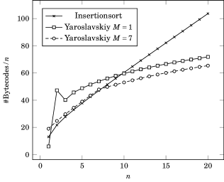
Figure 2: The expected number of executed Bytecodes for InsertionSort and Yaroslavskiy’s algorithm with different choices for $M$. The numbers of Bytecodes shown are normalized by $n$, i. e., we show the number of executed Bytecode instructions per element to be sorted. The data was obtained by naïvely evaluating the recurrence.

The overall linear term for the expected number of comparisons is

$$\bigl{(}\tfrac{124}{75}+\tfrac{3}{20}M-\tfrac{37}{10(M+2)}-\tfrac{62+19M}{10(M+2)}\mathcal{H}_{M+1}\bigr{)}(n+1)\;.$$

This coefficient has a proper minimum at $M=5$ with value $-3.62024\ldots$ . Compared with $-711\mathbin{/}200=-3.555$ for $M=1$ this a minor improvement though.

For the number of write operations, the linear term is

$$\bigl{(}\tfrac{86}{75}+\tfrac{3}{20}M-\tfrac{26}{5(M+2)}+\tfrac{18}{5(M+1)}-\tfrac{11}{10}\mathcal{H}_{M+2}\bigr{)}(n+1)\;.$$

The minimum $-1.098\overline{3}$ of this coefficient is also located at $M=5$. The corresponding coefficient for $M=1$ is $-0.695$. This improvement is more satisfying than the one for comparisons.

The linear term for the number of executed Bytecodes of Yaroslavskiy’s algorithm with $M\geq 2$ attains its minimum $-16.0887\ldots$ at $M=7$. This is a significant reduction over $-9.965\ldots$, the linear term without InsertionSorting. Figure 2 shows the resulting expected number of Bytecodes for small lists. For $n\leq 20$, using InsertionSort results in an improvement of over $10\,\%$. For $n=100$ we save $6.3\,\%$, for $n=1000$ it is $4.2\,\%$ and for $n=10\,000$, we still execute $3.1\,\%$ less Bytecode instructions than the basic version of Yaroslavskiy’s algorithm.

It is interesting to see that both elementary operations favor $M=5$, but the overall Bytecode count is minimized for “much” larger $M=7$. This shows that focusing on elementary operations can skew the view of an algorithm’s performance. Only explicitly taking the overhead of partitioning into account reveals that InsertionSort is significantly faster on small subproblems.

Remark

The actual Java 7 runtime library implementation uses $M=46$, which seems far from optimal at first sight. Note however that the implementation uses the more elaborate pivot selection scheme tertiles of five [Wild et al., 2013], which implies additional constant overhead per partitioning step.

4 Distribution of Costs

In this section we study the asymptotic distributions of our cost measures. We derive limit laws after normalization and identify the order of variances and covariances. In particular, we find that all costs are asymptotically concentrated around their mean.

As we confine ourselves to asymptotic statements of first order (leading terms in the expansions of variances and covariances), it turns out that the choice of $M$ does not affect the results of this section: All results hold for any (constant) $M$ (see [Neininger, 2001, proof of Corollary 5.5] for similar universal behavior of standard Quicksort). Appendix E shows that the asymptotic results are good approximations for practical input sizes $n$. A general survey on distributional analysis of various sorting algorithms covering many classical results is found in [Mahmoud, 2000].

4.1 The Contraction Method

Our tool to identify asymptotic variances, correlations and limit laws is the contraction method, which is applicable to many divide-and-conquer algorithms. Roughly speaking, the idea is to appropriately normalize a recurrence equation for the distribution of costs such that we can hope for convergence to a limit distribution. If we then replace all terms that depend on $n$ by their limits for $n\to\infty$, we obtain a map within the space of probability distributions that approximates the recurrence.

Next a (complete) metric between probability distributions is chosen such that this map becomes a contraction; then the Banach fixed-point theorem implies the existence of a unique fixed point for this map. This fixed point is the candidate for the limit distribution of the normalized costs and the underlying contraction property is then exploited to also show convergence of the normalized costs towards the fixed point. This convergence is shown within the same complete metric. If the metric is sufficiently strong, it may imply more than convergence in law; in our case we additionally obtain convergence of the first two moments, i. e., convergence of mean and variance. This enables us to compute asymptotics for the variance of the cost as well. Note that a fixed-point representation for a limit distribution is implicit, but it is suitable to compute moments of the limit distribution and to identify further properties such as the existence of a (Lebesgue) density.

For the reader’s convenience we formulate a general convergence theorem from the contraction method that is used repeatedly below and sufficient for our purpose. Let $(X_{n})_{n\geq 0}$ denote a sequence of centered and square integrable random variables either in $\mathbb{R}$ or $\mathbb{R}^{2}$ whose distributions satisfy the recurrence

$$X_{n} \mathrel{\;\;{\mathchoice{\mathrel{\overset{\raisebox{0.0pt}{$\scriptstyle\cal D$}}{=}}}{\mathrel{\hbox{\makebox[7.7778pt][c]{\makebox[0.0pt][c]{$\overset{\raisebox{-4.30554pt}{$\scriptscriptstyle\cal D$}}{=}$}}}}}{\mathrel{\overset{\cal D}{=}}}{\mathrel{\overset{\cal D}{=}}}}\;\;}\sum_{r=1}^{K}A^{\smash{(n)}}_{r}X^{\smash{(r)}}_{I^{(n)}_{r}}+b^{\smash{(n)}},\qquad n\geq n_{0},$$ (4.1)

where the random variables $(A^{\smash{(n)}}_{1},\ldots,A^{\smash{(n)}}_{K},b^{\smash{(n)}},I^{\smash{(n)}})$ and $(X^{\smash{(1)}}_{n})_{n\geq 0},\ldots,(X^{\smash{(K)}}_{n})_{n\geq 0}$ are independent, and $X^{\smash{(r)}}_{i}$ is distributed as $X_{i}$ for all $r=1,\ldots,K$ and $i\geq 0$. Furthermore, $I^{\smash{(n)}}=(I^{\smash{(n)}}_{1},\ldots,I^{\smash{(n)}}_{K})$ is a vector of random integers in $\{0,\ldots,n-1\}$ and $K$ and $n_{0}$ are fixed integers.

The coefficients $A^{\smash{(n)}}_{r}$ and $b^{\smash{(n)}}$ are real random variables in the univariate case, respectively random $2\times 2$ matrices and a $2$-dimensional random vector in the bivariate case. We assume also that the coefficients are square integrable and that the following conditions hold:

1. $(A^{\smash{(n)}}_{1},\ldots,A^{\smash{(n)}}_{K},b^{\smash{(n)}})\mathrel{\;{\stackrel{{\scriptstyle\ell_{2}}}{{\longrightarrow}}}\;}(A_{1},\ldots,A_{k},b)$,

2. $\sum_{r=1}^{K}\mathop{\mbox{$\mathbb{E}$}}\nolimits\left[\|A_{r}^{t}A_{r}\|_{\mathrm{op}}\right]\mathrel{\;{<}\;}1$,

3. $\sum_{r=1}^{K}\mathop{\mbox{$\mathbb{E}$}}\nolimits\bigl{[}{\bf 1}_{\{I^{\smash{(n)}}_{r}\leq\ell\}}\|(A^{\smash{(n)}}_{r})^{t}A^{\smash{(n)}}_{r}\|_{\mathrm{op}}\bigr{]}\mathrel{\;\;{\to}\;\;}0\mbox{ as }n\to\infty\mbox{ for all constants }\ell\geq 0$.

Here $\|A\|_{\mathrm{op}}\colonequals\sup_{\|x\|=1}\|Ax\|$ denotes the operator norm of a matrix and $A^{t}$ the transposed matrix. Note that in the univariate case we just have $\|A_{r}^{t}A_{r}\|_{\mathrm{op}}=A_{r}^{2}$. In (A) we denote by $\overset{\mbox{\smash{$\scriptscriptstyle\ell_{2}$}}}{\longrightarrow}$ convergence in the Wasserstein-metric of order 2 which here is equivalent to the existence of vectors $(\tilde{A}^{\smash{(n)}}_{1},\ldots,\tilde{A}^{\smash{(n)}}_{K},\tilde{b}^{\smash{(n)}})$ with the distribution of $(A^{\smash{(n)}}_{1},\ldots,A^{\smash{(n)}}_{K},b^{\smash{(n)}})$ such that we have the $L_{2}$ convergence

$$(\tilde{A}^{\smash{(n)}}_{1},\ldots,\tilde{A}^{\smash{(n)}}_{K},\tilde{b}^{\smash{(n)}}) \mathrel{\;\;{\stackrel{{\scriptstyle L_{2}}}{{\longrightarrow}}}\;\;}(A_{1},\ldots,A_{k},b)\;.$$

Note in particular that $A_{1},\ldots,A_{k},b$ are square integrable as well. Then we consider distributions of $X$ such that

$$X \mathrel{\;\;{\mathchoice{\mathrel{\overset{\raisebox{0.0pt}{$\scriptstyle\cal D$}}{=}}}{\mathrel{\hbox{\makebox[7.7778pt][c]{\makebox[0.0pt][c]{$\overset{\raisebox{-4.30554pt}{$\scriptscriptstyle\cal D$}}{=}$}}}}}{\mathrel{\overset{\cal D}{=}}}{\mathrel{\overset{\cal D}{=}}}}\;\;}\sum_{r=1}^{K}A_{r}X^{\smash{(r)}}+b\,,$$ (4.2)

where $(A_{1},\ldots,A_{K},b)$, $X^{\smash{(1)}},\ldots,X^{\smash{(K)}}$ are independent and $X^{\smash{(r)}}$ are distributed as $X$ for $r=1,\ldots,K$. The following two results from the contraction method are used:

1. Under (B), among all centered, square integrable distributions there is a unique solution ${\cal L}(X)$ to (4.2).

2. Assuming (A), (B) and (C), the sequence $(X_{n})_{n\geq 0}$ converges in distribution to the solution ${\cal L}(X)$ from (I). The convergence holds as well for the second (mixed) moments of $X_{n}$.

These results are given by Rösler [2001, Theorem 3] for the univariate case and Neininger [2001, Theorem 4.1] for the multivariate case.

4.2 Distributional Analysis of Yaroslavskiy’s Algorithm

We come back to Yaroslavskiy’s algorithm (Algorithm 1). To apply the contraction method, we have to characterize the full distribution of costs $T\!_{n}$ in one partitioning step and then formulate a distributional recurrence for the resulting distribution of costs $C_{n}$ for the complete sorting. To obtain a contracting mapping, we rewrite the derived recurrence for $C_{n}$ in terms of suitably normalized costs $C^{*}{}_{\mkern-13.0mun}\mkern 1.0mu$; here it will suffice to subtract the expected values computed in the last section and then to divide by $n$.

For the distributional analysis, it proves more convenient to consider i. i. d. uniformly on $[\mskip 1.0mu0,1]$ distributed random variables $U_{1},\ldots,U_{n}$ as input. Note that $U_{1},\dots,U_{n}$ are thus pairwise different almost surely. As the actual element values do not matter, this input model is the same as considering a random permutation.

Yaroslavskiy’s algorithm chooses $U_{1}$ and $U_{n}$ as pivot elements. Denote by $D=(D_{1},D_{2},D_{3})$ the spacings induced by $U_{1}$ and $U_{n}$ on the interval $[\mskip 1.0mu0,1]$; formally we have

$$(D_{1},D_{2},D_{3}) \mathrel{\;\;{=}\;\;}(U_{(1)},\,U_{(2)}-U_{(1)},\,1-U_{(2)})\,,$$

for $U_{(1)}\colonequals\min\{U_{1},U_{n}\}$ and $U_{(2)}\colonequals\max\{U_{1},U_{n}\}$. It is well-known that $D$ is uniformly distributed in the standard $2$-simplex [David and Nagaraja, 2003, p. 133f], i. e., $(D_{1},D_{2})$ has density

$$f_{D}(x_{1},x_{2}) \mathrel{\;\;{=}\;\;}\begin{cases}2,&\text{for }x_{1},x_{2}\geq 0\mathrel{\>{\wedge}\>}x_{1}+x_{2}\leq 1;\\ 0,&\text{otherwise},\end{cases}$$

and $D_{3}=1-D_{1}-D_{2}$ is fully determined by $(D_{1},D_{2})$. Hence, for a measurable function $g:[\mskip 1.0mu0,1]^{3}\to\mathbb{R}$ such that $g(D_{1},D_{2},D_{3})$ is integrable, we have that

$$\mathop{\mbox{$\mathbb{E}$}}\nolimits[g(D_{1},D_{2},D_{3})] \mathrel{\;\;{=}\;\;}2\int_{0}^{1}\mkern-6.0mu\int_{0}^{1-x_{1}}\!\!\!\!\!g(x_{1},x_{2},1-x_{1}-x_{2})\;dx_{2}\>dx_{1}\;.$$ (4.3)

Further we denote the sizes of the three subproblems generated in the first partitioning phase by $I^{\smash{(n)}}=(I^{\smash{(n)}}_{1},I^{\smash{(n)}}_{2},I^{\smash{(n)}}_{3})$. Then we have $I^{\smash{(n)}}_{1}+I^{\smash{(n)}}_{2}+I^{\smash{(n)}}_{3}=n-2$. Moreover, the spacings $D_{1}$, $D_{2}$ and $D_{3}$ are exactly the probabilities for an element $U_{i}$ ($1<i<n$) to be small, medium or large, respectively. As all these elements are independent, the vector $I^{\smash{(n)}}$, conditional on $D$, has a multinomial distribution:

$$I^{\smash{(n)}} \mathrel{\;\;{\mathchoice{\mathrel{\overset{\raisebox{0.0pt}{$\scriptstyle\cal D$}}{=}}}{\mathrel{\hbox{\makebox[7.7778pt][c]{\makebox[0.0pt][c]{$\overset{\raisebox{-4.30554pt}{$\scriptscriptstyle\cal D$}}{=}$}}}}}{\mathrel{\overset{\cal D}{=}}}{\mathrel{\overset{\cal D}{=}}}}\;\;}\mathrm{M}(n-2;\,D_{1},D_{2},D_{3}).$$

We will use the short notation $I^{\smash{(n)}}=I=(I_{1},I_{2},I_{3})$ when the dependence on $n$ is obvious. From the strong law of large numbers and dominated convergence we have in particular for $r\in\{1,2,3\}$

$$\frac{I_{r}^{\smash{(n)}}}{n} \mathrel{\;\;{\stackrel{{\scriptstyle L_{p}}}{{\longrightarrow}}}\;\;}D_{r}\qquad(n\to\infty),\quad\;1\leq p<\infty\;.$$ (4.4)

The advantage of this random model is that we can decouple values from ranks of pivots. With $D_{1}=U_{(1)}$ and $D_{1}+D_{2}=U_{(2)}$, we choose the values of the two pivots; however, the ranks $P$ and $Q$ are not yet fixed. Therefore given fixed pivot values, we can still independently draw non-pivot elements (with probabilities $D_{1}$, $D_{2}$ and $D_{3}$ to become small, medium and large, resp.), without having to fuzz with a priori restrictions on the overall number of small, medium and large elements. This makes it much easier to compute cost contributions uniformly in pivot values than in pivot ranks. If we operate on random permutations of $\{1,\ldots,n\}$, values and ranks coincide, so fixing pivot values there implies strict bounds on the number of small, medium and large elements.

4.2.1 Distribution of Toll Functions

Quantity Distribution given $I=(I_{1},I_{2},I_{3})$ |$P$ $=$ $I_{1}+1$ |$Q$ $=$ $n-I_{3}$ |$\delta$ $=$ $\mathbb{1}_{\{\smash{\raisebox{-0.2pt}{\scalebox{1.25}[1.18]{$\mathtt{A}$}}}[Q]>Q\}}$ $\mathchoice{\mathrel{\overset{\raisebox{0.0pt}{$\scriptstyle\cal D$}}{=}}}{\mathrel{\hbox{\makebox[7.00002pt][c]{\makebox[0.0pt][c]{$\overset{\raisebox{-3.87498pt}{$\scriptscriptstyle\cal D$}}{=}$}}}}}{\mathrel{\overset{\cal D}{=}}}{\mathrel{\overset{\cal D}{=}}}$ $\mathrm{B}\bigl{(}\tfrac{I_{3}}{n-2}\bigr{)}$ |$T_{\!A}$ $=$ $1$ |$T_{\!B}$ $=$ $\mathbb{1}_{\{\smash{\raisebox{-0.2pt}{\scalebox{1.25}[1.18]{$\mathtt{A}$}}}[\mathit{left}]>\smash{\raisebox{-0.2pt}{\scalebox{1.25}[1.18]{$\mathtt{A}$}}}[\mathit{right}]\}}$ $\mathchoice{\mathrel{\overset{\raisebox{0.0pt}{$\scriptstyle\cal D$}}{=}}}{\mathrel{\hbox{\makebox[7.00002pt][c]{\makebox[0.0pt][c]{$\overset{\raisebox{-3.87498pt}{$\scriptscriptstyle\cal D$}}{=}$}}}}}{\mathrel{\overset{\cal D}{=}}}{\mathrel{\overset{\cal D}{=}}}$ $\mathrm{B}\bigl{(}\tfrac{1}{2}\bigr{)}$ |$T_{\!F}$ $=$ $\delta$ $\mathchoice{\mathrel{\overset{\raisebox{0.0pt}{$\scriptstyle\cal D$}}{=}}}{\mathrel{\hbox{\makebox[7.00002pt][c]{\makebox[0.0pt][c]{$\overset{\raisebox{-3.87498pt}{$\scriptscriptstyle\cal D$}}{=}$}}}}}{\mathrel{\overset{\cal D}{=}}}{\mathrel{\overset{\cal D}{=}}}$ $\mathrm{B}\bigl{(}\tfrac{I_{3}}{n-2}\bigr{)}$ |$T_{\!C^{\smash{(1)}}}$ $=$ $Q-2+\delta$ $\mathchoice{\mathrel{\overset{\raisebox{0.0pt}{$\scriptstyle\cal D$}}{=}}}{\mathrel{\hbox{\makebox[7.00002pt][c]{\makebox[0.0pt][c]{$\overset{\raisebox{-3.87498pt}{$\scriptscriptstyle\cal D$}}{=}$}}}}}{\mathrel{\overset{\cal D}{=}}}{\mathrel{\overset{\cal D}{=}}}$ $I_{1}+I_{2}+\mathrm{B}\bigl{(}\tfrac{I_{3}}{n-2}\bigr{)}$ |$T_{\!C^{\smash{(3)}}}$ $=$ $n-Q$ $\mathchoice{\mathrel{\overset{\raisebox{0.0pt}{$\scriptstyle\cal D$}}{=}}}{\mathrel{\hbox{\makebox[7.00002pt][c]{\makebox[0.0pt][c]{$\overset{\raisebox{-3.87498pt}{$\scriptscriptstyle\cal D$}}{=}$}}}}}{\mathrel{\overset{\cal D}{=}}}{\mathrel{\overset{\cal D}{=}}}$ $I_{3}$ |$T_{\!C^{\smash{(4)}}}$ $=$ $\delta+(sm\mskip 1.0mu\mbox{\emph{@}}\mskip 1.0mu\mathcal{G})$ $\mathchoice{\mathrel{\overset{\raisebox{0.0pt}{$\scriptstyle\cal D$}}{=}}}{\mathrel{\hbox{\makebox[7.00002pt][c]{\makebox[0.0pt][c]{$\overset{\raisebox{-3.87498pt}{$\scriptscriptstyle\cal D$}}{=}$}}}}}{\mathrel{\overset{\cal D}{=}}}{\mathrel{\overset{\cal D}{=}}}$ $\mathrm{B}\bigl{(}\tfrac{I_{3}}{n-2}\bigr{)}+\mathrm{HypG}(I_{1}+I_{2},I_{3},n-2)$ |$T_{\!S^{\smash{(1)}}}$ $=$ $s\mskip 1.0mu\mbox{\emph{@}}\mskip 1.0mu\mathcal{K}$ $\mathchoice{\mathrel{\overset{\raisebox{0.0pt}{$\scriptstyle\cal D$}}{=}}}{\mathrel{\hbox{\makebox[7.00002pt][c]{\makebox[0.0pt][c]{$\overset{\raisebox{-3.87498pt}{$\scriptscriptstyle\cal D$}}{=}$}}}}}{\mathrel{\overset{\cal D}{=}}}{\mathrel{\overset{\cal D}{=}}}$ $\mathrm{HypG}(I_{1},I_{1}+I_{2},n-2)$ |$T_{\!S^{\smash{(3)}}}$ $=$ $P-1-(s\mskip 1.0mu\mbox{\emph{@}}\mskip 1.0mu\mathcal{K})$ $\mathchoice{\mathrel{\overset{\raisebox{0.0pt}{$\scriptstyle\cal D$}}{=}}}{\mathrel{\hbox{\makebox[7.00002pt][c]{\makebox[0.0pt][c]{$\overset{\raisebox{-3.87498pt}{$\scriptscriptstyle\cal D$}}{=}$}}}}}{\mathrel{\overset{\cal D}{=}}}{\mathrel{\overset{\cal D}{=}}}$ $I_{1}-\mathrm{HypG}(I_{1},I_{1}+I_{2},n-2)$

Table 3: Exact distributions of the toll functions introduced in Section 3.2 or equivalently the distributions of block execution frequencies in the first partitioning step.

In Section 3.2, we determined for each basic block of Yaroslavskiy’s algorithm, how often it is executed in one partitioning step. There, we only used the expected values in the end, but we already characterized the full distributions in passing. They are summarized in Table 3 for reference.

Most of those distributions are in fact mixed distributions, i. e., their parameters depend on the random variable $I=(I_{1},I_{2},I_{3})$, namely the sizes of the subproblems for recursive calls. For example, we find that $\delta$ conditional on the event $(I_{1},I_{2},I_{3})=(i_{1},i_{2},i_{3})$ is Bernoulli $\mathrm{B}(i_{3}\mathbin{/}(n-2))$ distributed, which we briefly write as $\delta\mathrel{\smash{\mathchoice{\mathrel{\overset{\raisebox{0.0pt}{$\scriptstyle\cal D$}}{=}}}{\mathrel{\hbox{\makebox[7.7778pt][c]{\makebox[0.0pt][c]{$\overset{\raisebox{-4.30554pt}{$\scriptscriptstyle\cal D$}}{=}$}}}}}{\mathrel{\overset{\cal D}{=}}}{\mathrel{\overset{\cal D}{=}}}}}\mathrm{B}(I_{3}\mathbin{/}(n-2))$. Note that since $I$ has itself a mixed distribution — namely conditional on $D$ — we actually have three layers of random variables: spacings, subproblem sizes and toll functions. The key technical lemmas for dealing with these three-layered distributions are given in Section 4.3.

4.2.2 Distributional Recurrence

Denote by $T\!_{n}$ the (random) costs of the first partitioning step of Yaroslavskiy’s algorithm. By Property 2.1, subproblems generated in the first partitioning phase are, conditional on their sizes, again uniformly random permutations and independent of each other. Hence, we obtain the distributional recurrence for the (random) total costs $C_{n}$:

$$C_{n}\mathrel{\;\;{\mathchoice{\mathrel{\overset{\raisebox{0.0pt}{$\scriptstyle\cal D$}}{=}}}{\mathrel{\hbox{\makebox[7.7778pt][c]{\makebox[0.0pt][c]{$\overset{\raisebox{-4.30554pt}{$\scriptscriptstyle\cal D$}}{=}$}}}}}{\mathrel{\overset{\cal D}{=}}}{\mathrel{\overset{\cal D}{=}}}}\;\;}C^{\prime}_{I_{1}}+C^{\prime\prime}_{I_{2}}+C^{\prime\prime\prime}_{I_{3}}\mathbin{\;{+}\;}T\!_{n}\,,\qquad(n\geq 3),$$ (4.5)

where $(I_{1},I_{2},I_{3},T\!_{n})$, $(C_{j}{}^{\mkern-10.0mu\prime}\mkern 3.0mu)_{j\geq 0}$, $(C_{\!j\,}{}^{\mkern-10.0mu\prime\prime}\mkern 1.0mu)_{j\geq 0}$, $(C_{\!j\,}{}^{\mkern-10.0mu\prime\prime\prime}\mkern 1.0mu)_{j\geq 0}$ are independent and $C_{j}{}^{\mkern-10.0mu\prime}\mkern 3.0mu$, $C_{\!j\,}{}^{\mkern-10.0mu\prime\prime}\mkern 1.0mu$, $C_{\!j\,}{}^{\mkern-10.0mu\prime\prime\prime}\mkern 1.0mu$ are identically distributed as $C_{j}$ for $j\geq 0$. By Theorems 3.8, 3.9 and 3.10, we know the expected costs $\mathop{\mbox{$\mathbb{E}$}}\nolimits[C_{n}]$, so with $C^{*}_{0}\colonequals 0$ and

$$C^{*}_{n} \mathrel{\;\;{\colonequals}\;\;}\frac{C_{n}-\mathop{\mbox{$\mathbb{E}$}}\nolimits[C_{n}]}{n}\,,\qquad\text{for }n\geq 1,$$ (4.6)

we have a sequence $(C^{*}{}_{\mkern-13.0mun}\mkern 1.0mu)_{n\geq 0}$ of centered, square integrable random variables. Using (4.5) we find, cf. [Hwang and Neininger, 2002, eq. (27), (28)], that $(C^{*}{}_{\mkern-13.0mun}\mkern 1.0mu)_{n\geq 0}$ satisfies (4.1) with

$$A^{\smash{(n)}}_{r} \mathrel{\;\;{=}\;\;}\frac{I_{r}}{n}, b^{\smash{(n)}} \mathrel{\;\;{=}\;\;}\frac{1}{n}\biggl{(}T\!_{n}-\mathop{\mbox{$\mathbb{E}$}}\nolimits[C_{n}]\mathbin{\;{+}\;}\sum_{r=1}^{3}\mathop{\mbox{$\mathbb{E}$}}\nolimits[C_{I_{r}}\mathbin{\mid}I_{r}]\biggr{)}\,,$$ (4.7)

so we can apply the framework of the contraction method. It remains to check the conditions (A), (B) and (C) to prove that $C^{*}{}_{\mkern-13.0mun}\mkern 1.0mu$ indeed converges to a limit law; the detailed computations are given in Appendix D. The key results needed therein are presented in the following section as technical lemmas.

4.3 Asymptotics of Mixed Distributions

The following convergence results for mixed distributions are essential for proving condition (A).

Lemma 4.1.

Let $(V_{1},\ldots,V_{b})$ be a vector of random probabilities, i. e., $0\leq V_{r}\leq 1$ for all $r=1,\ldots,b$ and $\sum_{r=1}^{b}V_{r}=1$ almost surely. Let

$$(L_{1},\ldots,L_{b})\mathrel{\;\;{\colonequals}\;\;}(L^{\smash{(n)}}_{1},\ldots,L^{\smash{(n)}}_{b})\mathrel{\;\;{\mathchoice{\mathrel{\overset{\raisebox{0.0pt}{$\scriptstyle\cal D$}}{=}}}{\mathrel{\hbox{\makebox[7.7778pt][c]{\makebox[0.0pt][c]{$\overset{\raisebox{-4.30554pt}{$\scriptscriptstyle\cal D$}}{=}$}}}}}{\mathrel{\overset{\cal D}{=}}}{\mathrel{\overset{\cal D}{=}}}}\;\;}\mathrm{M}(n;V_{1},\ldots,V_{b}),$$ (4.8)

be mixed multinomially distributed. Furthermore for $J_{1},J_{2}\subset\{1,\ldots,b\}$ let

$$Z_{n}\mathrel{\;\;{\mathchoice{\mathrel{\overset{\raisebox{0.0pt}{$\scriptstyle\cal D$}}{=}}}{\mathrel{\hbox{\makebox[7.7778pt][c]{\makebox[0.0pt][c]{$\overset{\raisebox{-4.30554pt}{$\scriptscriptstyle\cal D$}}{=}$}}}}}{\mathrel{\overset{\cal D}{=}}}{\mathrel{\overset{\cal D}{=}}}}\;\;}\mathrm{HypG}\biggl{(}\sum_{j\in J_{1}}L_{j},\;\sum_{j\in J_{2}}L_{j},\;n\biggr{)}$$ (4.9)

be mixed hypergeometrically distributed. Then we have the $L_{2}$-convergence, as $n\to\infty$,

$$\frac{Z_{n}}{n} \mathrel{\;\;{\stackrel{{\scriptstyle L_{2}}}{{\longrightarrow}}}\;\;}\biggl{(}\sum_{j\in J_{1}}\!V_{j}\biggr{)}\cdot\biggl{(}\sum_{j\in J_{2}}\!V_{j}\biggr{)}.$$ (4.10)

The proof exploits that the binomial and the hypergeometric distributions are both strongly concentrated around their means. The full-detail computations to lift this to conditional expectations are given in Appendix D.

Lemma 4.2.

For $L_{1},\ldots,L_{b}$ from Lemma 4.1, we have for $1\leq i\leq b$ the $L_{2}$-convergence

$$\tfrac{L_{i}}{n}\ln\bigl{(}\tfrac{L_{i}}{n}\bigr{)} \mathrel{\;\;{\stackrel{{\scriptstyle L_{2}}}{{\longrightarrow}}}\;\;}V_{i}\ln(V_{i})\,,\qquad\text{as }n\to\infty.$$ (4.11)

(Recall that we set $x\ln(x)\colonequals 0$ for $x=0$.)
The proof is directly obtained by combining the law of large numbers with the dominated convergence theorem; see Appendix D for details.

4.4 Key Comparisons

We have the following asymptotic results on the variance and distribution of the number of key comparisons of Yaroslavskiy’s algorithm:

Theorem 4.3.

For the number $C_{n}$ of key comparisons used by Yaroslavskiy’s Quicksort when operating on a uniformly at random distributed permutation we have

$$\frac{C_{n}-\mathop{\mbox{$\mathbb{E}$}}\nolimits[C_{n}]}{n} \mathrel{\;\;{\to}\;\;}C^{*},\qquad(n\to\infty),$$ (4.12)

where the convergence is in distribution and with second moments. The distribution of $C^{*}$ is determined as the unique fixed point, subject to $\mathop{\mbox{$\mathbb{E}$}}\nolimits[X]=0$ and $\mathop{\mbox{$\mathbb{E}$}}\nolimits[X^{2}]<\infty$, of

$$X \mathrel{\;\;{\mathchoice{\mathrel{\overset{\raisebox{0.0pt}{$\scriptstyle\cal D$}}{=}}}{\mathrel{\hbox{\makebox[7.7778pt][c]{\makebox[0.0pt][c]{$\overset{\raisebox{-4.30554pt}{$\scriptscriptstyle\cal D$}}{=}$}}}}}{\mathrel{\overset{\cal D}{=}}}{\mathrel{\overset{\cal D}{=}}}}\;\;}1\mathbin{\>{+}\>}(D_{1}+D_{2})(D_{2}+2D_{3})\mathbin{\;{+}\;}\sum_{j=1}^{3}\left(D_{j}X^{\smash{(j)}}+\tfrac{19}{10}D_{j}\ln D_{j}\right)\,,$$ (4.13)

where $(D_{1},D_{2},D_{3})$, $X^{\smash{(1)}}$, $X^{\smash{(2)}}$ and $X^{\smash{(3)}}$ are independent and $X^{\smash{(j)}}$ has the same distribution as $X$ for $j\in\{1,2,3\}$. Moreover, we have, as $n\to\infty$,

$$\mathrm{Var}(C_{n}) \mathrel{\;\;{\sim}\;\;}\sigma_{C}^{2}n^{2}\qquad\quad\text{with}\qquad\quad\sigma_{C}^{2}\mathrel{\;\;{=}\;\;}\tfrac{2231}{360}-\tfrac{361}{600}\pi^{2}=0.25901\!\ldots$$ (4.14)

For the proof, we apply the contraction method to $X_{n}=C^{*}{}_{\mkern-13.0mun}\mkern 1.0mu$ as defined by (4.6), where the toll function $T_{\!C}({n})$ is used. Details on checking conditions (A), (B) and (C), as well as the derivation of the resulting fixed-point equation for $C^{*}$ and the computation of the variance are given in Appendix D.

4.5 Swaps

For the number of swaps in Yaroslavskiy’s algorithm we have the following asymptotic behavior of variance and distribution.

Theorem 4.4.

For the number $S_{n}$ of swaps used by Yaroslavskiy’s algorithm when operating on a random permutation we have

$$\frac{S_{n}-\mathop{\mbox{$\mathbb{E}$}}\nolimits[S_{n}]}{n} \mathrel{\;\;{\to}\;\;}S^{*}\,,\qquad(n\to\infty)\,,$$ (4.15)

where the convergence is in distribution and with second moments. The distribution of $S^{*}$ is determined as the unique fixed point, subject to $\mathop{\mbox{$\mathbb{E}$}}\nolimits[X]=0$ and $\mathop{\mbox{$\mathbb{E}$}}\nolimits[X^{2}]<\infty$, of

$$X \mathrel{\;\;{\mathchoice{\mathrel{\overset{\raisebox{0.0pt}{$\scriptstyle\cal D$}}{=}}}{\mathrel{\hbox{\makebox[7.7778pt][c]{\makebox[0.0pt][c]{$\overset{\raisebox{-4.30554pt}{$\scriptscriptstyle\cal D$}}{=}$}}}}}{\mathrel{\overset{\cal D}{=}}}{\mathrel{\overset{\cal D}{=}}}}\;\;}D_{1}\mathbin{\>{+}\>}(D_{1}+D_{2})\,D_{3}\mathbin{\;{+}\;}\sum_{j=1}^{3}\left(D_{j}X^{\smash{(j)}}+\tfrac{3}{5}D_{j}\ln D_{j}\right)\,,$$ (4.16)

where $(D_{1},D_{2},D_{3})$, $X^{\smash{(1)}}$, $X^{\smash{(2)}}$ and $X^{\smash{(3)}}$ are independent and $X^{\smash{(j)}}$ has the same distribution as $X$ for $j\in\{1,2,3\}$. Moreover, we have, as $n\to\infty$,

$$\mathrm{Var}(S_{n}) \mathrel{\;\;{\sim}\;\;}\sigma_{S}^{2}n^{2},\qquad\text{with}\qquad\sigma_{S}^{2}\mathrel{\;\;{=}\;\;}\tfrac{7}{10}-\tfrac{3}{50}\pi^{2}\mathrel{\;\;{=}\;\;}0.10782\!\ldots$$ (4.17)

The proof is similar to the one for Theorem 4.3, details are given in Appendix D.

4.6 Executed Bytecode Instructions

For the number of executed Java Bytecode instructions in Yaroslavskiy’s algorithm we have the following asymptotic variance and distribution.

Theorem 4.5.

For the number $\mathit{BC}_{n}$ of executed Java Bytecodes used by Yaroslavskiy’s algorithm when sorting a random permutation, we have

$$\frac{\mathit{BC}_{n}-\mathop{\mbox{$\mathbb{E}$}}\nolimits[\mathit{BC}_{n}]}{n} \mathrel{\;\;{\to}\;\;}\mathit{BC}^{*}\,,\qquad(n\to\infty)\,,$$ (4.18)

where the convergence is in distribution and with second moments. The distribution of $\mathit{BC}^{*}$ is determined as the unique fixed point, subject to $\mathop{\mbox{$\mathbb{E}$}}\nolimits[X]=0$ and $\mathop{\mbox{$\mathbb{E}$}}\nolimits[X^{2}]<\infty$, of

$$X \mathrel{\;\;{\mathchoice{\mathrel{\overset{\raisebox{0.0pt}{$\scriptstyle\cal D$}}{=}}}{\mathrel{\hbox{\makebox[7.7778pt][c]{\makebox[0.0pt][c]{$\overset{\raisebox{-4.30554pt}{$\scriptscriptstyle\cal D$}}{=}$}}}}}{\mathrel{\overset{\cal D}{=}}}{\mathrel{\overset{\cal D}{=}}}}\;\;}24+(D_{3}-9)D_{2}-2D_{3}(5D_{3}+2)\mathbin{\;{+}\;}\sum_{j=1}^{3}\left(D_{j}X^{\smash{(j)}}+\tfrac{217}{10}D_{j}\ln D_{j}\right)\,,$$ (4.19)

where $(D_{1},D_{2},D_{3})$, $X^{\smash{(1)}}$, $X^{\smash{(2)}}$ and $X^{\smash{(3)}}$ are independent and $X^{\smash{(j)}}$ has the same distribution as $X$ for $j\in\{1,2,3\}$. Moreover, we have, as $n\to\infty$,

$$\mathrm{Var}(\mathit{BC}_{n}) \mathrel{\;\;{\sim}\;\;}\sigma_{\mathit{BC}}^{2}n^{2},\qquad\text{with}\qquad\sigma_{\mathit{BC}}^{2}\mathrel{\;\;{=}\;\;}\tfrac{1\,469\,983}{1\,800}-\tfrac{47\,089}{600}\pi^{2}\mathrel{\;\;{=}\;\;}42.0742\!\ldots$$ (4.20)

Again, the proof is similar to the one for Theorem 4.3 and details are given in Appendix D.

4.7 Covariance of Comparisons and Swaps

In this section we study the asymptotic covariance $\mathrm{Cov}(C_{n},S_{n})$ between the number of key comparisons $C_{n}$ and the number of swaps $S_{n}$ in Yaroslavskiy’s algorithm.

Theorem 4.6.

For the number $C_{n}$ of key comparisons and the number $S_{n}$ of swaps used by Yaroslavskiy’s algorithm on a random permutation, we have for $n\to\infty$

$$\mathrm{Cov}(C_{n},S_{n}) \mathrel{\;\;{\sim}\;\;}\sigma_{C,S}\,n^{2}\qquad\text{with}\qquad\sigma_{C,S}\mathrel{\;\;{=}\;\;}\tfrac{28}{15}-\tfrac{19}{100}\pi^{2}\mathrel{\;\;{=}\;\;}-0.00855817\!\ldots$$ (4.21)

The correlation coefficient of $C_{n}$ and $S_{n}$ consequently is

$$\frac{\mathrm{Cov}(C_{n},S_{n})}{\sqrt{\mathrm{Var}(C_{n})}\sqrt{\mathrm{Var}(S_{n})}}\mathrel{\;\;{\sim}\;\;}\rho\mathrel{\;\;{\approx}\;\;}-0.0512112\!\ldots$$

For the proof of Theorem 4.6, we consider the bivariate random variables $Y_{n}\colonequals\bigl{(}{C_{n}\atop S_{n}}\!\bigr{)}$ and show that their normalized versions $Y^{*}{}_{\mkern-17.0mun}\mkern 2.0mu\colonequals\tfrac{1}{n}\bigl{(}Y_{n}-\mathop{\mbox{$\mathbb{E}$}}\nolimits[Y_{n}]\bigr{)}$ converge to the (bivariate) distribution $\mathcal{L}(\Lambda_{1},\Lambda_{2})$, which is, as before, characterized as the unique fixed point of a distributional equation. The covariance of $C_{n}$ and $S_{n}$ is then obtained by multiplying both components of $Y^{*}{}_{\mkern-17.0mun}\mkern 2.0mu$, which converges to $\mathop{\mbox{$\mathbb{E}$}}\nolimits[\Lambda_{1}\cdot\Lambda_{2}]$. Full computations are found in Appendix D.

Note that Theorem 4.6 and its proof directly imply the asymptotic variance and limit distribution of all linear combinations $\alpha C_{n}+\beta S_{n}$, for $\alpha,\beta\in\mathbb{R}$, which are, for $\alpha,\beta>0$, natural cost measures when weighting key comparisons against swaps. The reason is that in the proof of Theorem 4.6 we show the bivariate limit law

$$\left(\frac{C_{n}-\mathop{\mbox{$\mathbb{E}$}}\nolimits[C_{n}]}{n},\frac{S_{n}-\mathop{\mbox{$\mathbb{E}$}}\nolimits[S_{n}]}{n}\right) \mathrel{\;\;{\to}\;\;}(\Lambda_{1},\Lambda_{2}),$$

which holds in distribution and with second mixed moments. Hence, the continuous mapping theorem implies, as $n\to\infty$,

$$\frac{\alpha C_{n}+\beta S_{n}\mathbin{\;{-}\;}(\alpha\mathop{\mbox{$\mathbb{E}$}}\nolimits[C_{n}]+\beta\mathop{\mbox{$\mathbb{E}$}}\nolimits[S_{n}])}{n} \mathrel{\;\;{\to}\;\;}\alpha\Lambda_{1}+\beta\Lambda_{2},$$

in distribution and with second moments. Thus, we obtain, as $n\to\infty$,

$$\mathrm{Var}(\alpha C_{n}+\beta S_{n}) \mathrel{\;\;{=}\;\;}\alpha^{2}\mathrm{Var}(C_{n})\mathbin{\>{+}\>}\beta^{2}\mathrm{Var}(S_{n})\mathbin{\>{+}\>}2\alpha\beta\,\mathrm{Cov}(C_{n},S_{n})$$

$$\mathrel{\;\;{\sim}\;\;}(\alpha^{2}\sigma^{2}_{C}+\beta^{2}\sigma^{2}_{S}+2\alpha\beta\,\sigma_{C,S})\,n^{2}.$$

Note that by this approach also the covariances between all the single contributions from Table 3 that contribute with linear order in the first partitioning step to the number of executed Java Bytecodes used by Yaroslavskiy’s algorithm can be identified asymptotically in first order.

5 Conclusion

In this paper, we conducted a fully detailed analysis of Yaroslavskiy’s dual-pivot Quicksort — including the optimization of using Insertionsort on small subproblems — in the style of Knuth’s book series The Art of Computer Programming. We give the exact expected number of executed Java Bytecode instructions for Yaroslavskiy’s algorithm. On top of the exact average case results, we establish existence and fixed-point characterizations of limiting distribution of normalized costs. From this, we compute moments of the limiting distributions, in particular the asymptotic variance of the number of executed Bytecodes. The mere fact that such a detailed average and distributional analysis is tractable, seems worth noting. For the reader’s convenience, we summarize the main results of this paper in Table 4, where we also cite corresponding results on classic single-pivot Quicksort for comparison.

Cost Measure Yaroslavskiy’s Quicksort Classic Quicksort error with $M=7$ with $M=6$ Comparisons expectation $\mathrm{O}(\log n)$ $1.9n\ln n\mathbin{-}2.49976n$ $2n\ln n\mathbin{-}2.3045n$tn:sedgewick77 std. dev. $o(n)$ $0.50893n$ $0.648278n$tn:hennequin89 Swaps (for $M=1$) expectation $\mathrm{O}(\log n)$ $0.6n\ln n\mathbin{-}0.107004n$ $0.\overline{3}n\ln n\mathbin{-}0.585373n$tn:sedgewick77 std. dev. $o(n)$ $0.328365n$ $0.0237251n$tn:hennequin89 Writes Accesses expectation $\mathrm{O}(\log n)$ $1.1n\ln n\mathbin{-}0.408039n$ $0.\overline{6}n\ln n\mathbin{+}0.316953n$tn:sedgewick77 Executed Bytecodes expectation $\mathrm{O}(\log n)$ $21.7n\ln n\mathbin{-}3.56319n$ $18n\ln n\mathbin{+}6.21488n$tn:bytecodes std. dev. $o(n)$ $6.48646n$ $3.52723n$tn:stdevBytecodes Correlation Coefficient for $o(1)$ $-0.0512112$ $-0.86404$tn:corr Comparisons and Swaps

• see [Sedgewick, 1977, p. 334].

• see [Hennequin, 1989, p. 330].

• see [Wild, 2012, p. 123].

• as in [Neininger, 2001, p. 515] for MIX,
  but with Bytecode costs of [Wild, 2012].

• see [Neininger, 2001, Table 1].

Table 4: Summary of the results of this paper and comparison with corresponding results for classic Quicksort. $M$ is chosen such that the number of executed Bytecodes in minimized. (For swaps, results for $M=1$ are given as Insertionsort is not swap-based.) Some asymptotic approximations have been weakened for conciseness of presentation, see the main text for full precision. The asymptotics use the well-known expansion of Harmonic Numbers [e. g. Graham et al. 1994, eq. (6.66)]

As observed by Wild and Nebel [2012], Yaroslavskiy’s algorithm uses $5$ % less key comparisons, but $80$ % more swaps in the asymptotic average than classic Quicksort. Unless comparisons are very expensive, one should expect classic Quicksort to be more efficient in total. This intuition is confirmed by our detailed analysis: In the asymptotic average, the Java implementation of Yaroslavskiy’s algorithm executes $20$ % more Java Bytecode instructions than a corresponding implementation of classic Quicksort.

Strengthening confidence in expectations, we find that asymptotic standard deviations of all costs remain linear in $n$; by Chebyshev’s inequality, this implies concentration around the mean. Whereas the number of comparisons in Yaroslavskiy’s algorithm shows slightly less variance than for classic Quicksort, swaps exhibit converse behavior. In fact, the number of swaps in classic Quicksort is highly concentrated because it already achieves close to optimal average behavior: In the partitioning step of classic Quicksort, every swap puts both elements into the correct partition and we never revoke a placement during one partitioning step. In contrast, in Yaroslavskiy’s algorithm every swap puts only one element into its final location (for the current partitioning step); the other element might have to be moved a second time later.

Another facet of this difference is revealed by considering the correlation coefficient between swaps and comparisons. In classic Quicksort, swaps and comparisons are almost perfectly negatively correlated. A “good” run w. r. t. comparisons needs balanced partitioning, but the more balanced partitioning becomes, the higher is the potential for misplaced elements that need to be moved. In Yaroslavskiy’s partitioning method, such a clear dependency does not exist for several reasons. First of all, even if pivots have extreme ranks, sometimes many swaps are done; e. g. if $p$ and $q$ are the two largest elements, all elements are swapped in our implementation. Secondly, for some pivot ranks, comparisons and swaps behave covariantly: For example if $p$ and $q$ are the two smallest elements, no swap is done and every element’s partition is found with one comparison only. In the end, the number of comparisons and swaps is almost uncorrelated in Yaroslavskiy’s algorithm.

The asymptotic standard deviation of the total number of executed Bytecode instructions is about twice as large in Yaroslavskiy’s algorithm as in classic Quicksort. This might be a consequence of the higher variability in the number of swaps just described.

Concerning practical performance, asymptotic behavior is not the full story. Often, inputs in practice are of moderate size and only the massive number of calls to a procedure makes it a bottleneck of overall execution. Then, lower order terms are not negligible. For Quicksort, this means in particular that constant overhead per partitioning step has to be taken into account. For tiny $n$, this overhead turns out to be so large, that it pays to switch to a simpler sorting method instead of Quicksort. We showed that using InsertionSort for subproblems of size at most $M$ speeds up Yaroslavskiy’s algorithm significantly for moderate $n$. The optimal choice for $M$ w. r. t. the number of executed Bytecodes is $M=7$.

Combining the results for InsertionSort from Appendix B and a corresponding Bytecode count analysis of a Java implementation of classic Quicksort [Wild, 2012], we can compare classic Quicksort and Yaroslavskiy’s algorithm exactly. As striking result we observe that in expectation, Yaroslavskiy’s algorithm needs more Java Bytecodes than classic Quicksort for all $n$. Thus, the efficiency of classic Quicksort in terms of executed Bytecodes is not just an effect of asymptotic approximations, it holds for realistic input sizes, as well.

These findings clearly contradict corresponding running time experiments [Wild, 2012, Chapter 8], where Yaroslavskiy’s algorithm was significantly faster across implementations and programming environments. One might object that the poor performance of Yaroslavskiy’s algorithm is a peculiarity of counting Bytecode instructions. Wild [2012, Section 7.1] also gives implementations and analyses thereof in MMIX, the new version of Knuth’s imaginary processor architecture. Every MMIX instruction has well-defined costs, chosen to closely resemble actual execution time on a simple processor. The results show the same trend: Classic Quicksort is more efficient. Together with the Bytecode results of this paper, we see strong evidence for the following conjecture:

Conjecture 5.1.

The efficiency of Yaroslavskiy’s algorithm in practice is caused by advanced features of modern processors. In models that assign constant cost contributions to single instructions — i. e., locality of memory accesses and instruction pipelining are ignored — classic Quicksort is more efficient.

It will be the subject of future investigations to identify the true reason of the success of Yaroslavskiy’s dual-pivot Quicksort.

APPENDIX

Appendix A Solving the Dual-Pivot Quicksort Recurrence

The proof presented in the following is basically a generalization of the derivation given by Sedgewick [1975, p. 156ff]. Hennequin [1991] gives an alternative approach based on generating functions that is much more general. Even though the authors consider Hennequin’s method elegant, we prefer the elementary proof, as it allows a self-contained presentation.

Two basic identities involving binomials and Harmonic Numbers are used several times below, so we collect them here. They are found as equations (6.70) and (5.10) in [Graham et al., 1994].

$$\sum_{0\leq k<n}\tbinom{k}{m}\mathcal{H}_{k} \mathrel{\;\;{=}\;\;}\tbinom{n}{m+1}\bigl{(}\mathcal{H}_{n}-\tfrac{1}{m+1}\bigr{)}\,, \text{integer }m\geq 0\,,$$ (A.1)

$$\sum_{0\leq k\leq n}\tbinom{k}{m} \mathrel{\;\;{=}\;\;}\tbinom{n+1}{m+1}\,, \text{integers }n,\,m\geq 0\;.$$ (A.2)

Proof of Theorem 3.1: The first step is to use symmetries of the sum in (3.2).

$$\sum_{1\leq p<q\leq n}\!\!\!\left(C_{p-1}+C_{q-p-1}+C_{n-q}\right)\mathrel{\;\;{=}\;\;} \sum_{p=1}^{n-1}(n-p)C_{p-1}\;\;+\;\;\sum_{k=0}^{n-2}(n-1-k)C_{k}\;\;+\;\;\sum_{q=2}^{n}(q-1)C_{n-q}$$

$$\mathrel{\;\;{=}\;\;} 3\sum_{k=0}^{n-2}(n-k-1)C_{k}\;.$$

So, our recurrence to solve is

$$C_{n} \mathrel{\;\;{=}\;\;}T\!_{n}+\tfrac{6}{n(n-1)}\sum_{k=0}^{n-2}(n-k-1)C_{k}\,,\qquad\mbox{for }n>M\;.$$ (A.3)

We first consider $D_{n}:=\tbinom{n+1}{2}C_{n+1}-\tbinom{n}{2}C_{n}$ to get rid of the factor in front of the sum:

$$D_{n} \mathrel{\;\;{=}\;\;}\overbrace{\tbinom{n+1}{2}T\!_{n+1}-\tbinom{n}{2}T\!_{n}}^{d(n)\colonequals}\qquad\qquad(n\geq M+2)$$

$$\mathrel{\;\;{\phantom{{}={}}}\;\;}{}+\tfrac{(n+1)n}{2}\tfrac{6}{(n+1)n}\sum_{k=0}^{n-1}(n-k)C_{k}\mathbin{\;\;{-}\;\;}\tfrac{n(n-1)}{2}\tfrac{6}{n(n-1)}\sum_{k=0}^{n-2}(n-k-1)C_{k}$$

$$\mathrel{\;\;{=}\;\;}d(n)\;+\;3\sum_{k=0}^{n-1}C_{k}\;.$$

The remaining full history recurrence is eliminated by taking ordinary differences

$$E_{n} \mathrel{\;{\colonequals}\;}D_{n+1}-D_{n}\mathrel{\;{=}\;}d(n+1)-d(n)+3C_{n}\;.\qquad(n\geq M+2)$$

Towards a telescoping recurrence, we consider $F_{n}\mathrel{\;{\colonequals}\;}C_{n}-\tfrac{n-4}{n}\cdot C_{n-1}\,,$ and compute

$$F_{n+2}-F_{n+1} \mathrel{\;\;{=}\;\;}C_{n+2}-\tfrac{n-2}{n+2}C_{n+1}-\left(C_{n+1}-\tfrac{n-3}{n+1}C_{n}\right)$$

$$\mathrel{\;\;{=}\;\;}C_{n+2}-\tfrac{2n}{n+2}C_{n+1}+\tfrac{n-3}{n+1}C_{n}\;.$$ (A.4)

The expression on the right hand side in itself is not helpful. However, by expanding the definition of $E_{n}$, we find

$$\left(E_{n}-3C_{n}\right)\bigm{/}\tbinom{n+2}{2} \mathrel{\;\;{=}\;\;}\left(D_{n+1}-D_{n}-3C_{n}\right)\bigm{/}\tbinom{n+2}{2}$$

$$\mathrel{\;\;{=}\;\;}\biggl{(}\tbinom{n+2}{2}C_{n+2}-\tbinom{n+1}{2}C_{n+1}-\left(\tbinom{n+1}{2}C_{n+1}-\tbinom{n}{2}C_{n}\right)-3C_{n}\biggr{)}\Big{/}\tbinom{n+2}{2}$$

$$\mathrel{\;\;{=}\;\;}C_{n+2}-\tfrac{2n}{n+2}C_{n+1}+\tfrac{\frac{1}{2}n(n-1)-3}{\frac{1}{2}(n+2)(n-1)}C_{n}$$

$$\mathrel{\;\;{=}\;\;}C_{n+2}-\tfrac{2n}{n+2}C_{n+1}+\tfrac{\frac{1}{2}(n-3)(n+2)}{\frac{1}{2}(n+2)(n-1)}C_{n}$$

$$\mathrel{\;\;{=}\;\;}C_{n+2}-\tfrac{2n}{n+2}C_{n+1}+\tfrac{n-3}{n+1}C_{n}\;.$$ (A.5)

Equating (A.4) and (A.5) yields

$$F_{n+2}-F_{n+1}\mathrel{\;{=}\;}\left(E_{n}-3C_{n}\right)\bigm{/}\tbinom{n+2}{2}\mathrel{\;{=}\;}\underbrace{\bigl{(}d(n+1)-d(n)\bigr{)}\bigm{/}\tbinom{n+2}{2}}_{f(n)\colonequals}\;.\quad(n\geq M+2)$$

This last equation is now amenable to simple iteration:

$$F_{n} \mathrel{\;{=}\;}\underbrace{\sum_{i=M+4}^{n}\!\!f(i-2)\mathbin{\;{+}\;}F_{M+3}}_{g(n)}\;.\qquad(n\geq M+4)$$

Plugging in the definition of $F_{n}=C_{n}-\frac{n-4}{n}\cdot C_{n-1}$ yields

$$C_{n}\mathrel{\;{=}\;}\tfrac{n-4}{n}\cdot C_{n-1}\mathbin{\;{+}\;}g(n)\;.\qquad(n\geq M+4)$$ (A.6)

Multiplying (A.6) by $\tbinom{n}{4}$ and using $\tbinom{n}{4}\cdot\frac{n-4}{n}=\tbinom{n-1}{4}$ gives a telescoping recurrence:

$$G_{n}\mathrel{\;{\colonequals}\;}\tbinom{n}{4}C_{n} \mathrel{\;\;{=}\;\;}G_{n-1}+\tbinom{n}{4}g(n)$$

$$\mathrel{\;\;{=}\;\;}\mkern-10.0mu\sum_{i=M+4}^{n}\mkern-5.0mu\tbinom{i}{4}g(i)\mathbin{\>{+}\>}G_{M+3}$$

$$\mathrel{\;\;{=}\;\;}\sum_{i=1}^{n}\tbinom{i}{4}g(i)\mathbin{\;{+}\;}G_{M+3}\mathbin{\;{-}\;}\sum_{i=1}^{M+3}\tbinom{i}{4}\biggl{(}\>\smash{\overbrace{\rule{0.0pt}{13.3472pt}\smash{\sum_{j=M+4}^{i}}f(j-2)}^{=\mskip 1.0mu0}}\mathbin{\;{+}\;}F_{M+3}\biggr{)}$$

$$\mathrel{\;\;{=}\;\;}\sum_{i=1}^{n}\tbinom{i}{4}g(i)\mathbin{\;{+}\;}G_{M+3}\mathbin{\;{-}\;}\tbinom{M+4}{5}F_{M+3}\,,$$ (A.7)

where the last equation uses (A.2). Applying definitions, we find

$$\sum_{i=1}^{n}\tbinom{i}{4}g(i) \mathrel{\;\;{=}\;\;}\sum_{i=1}^{n}\tbinom{i}{4}\biggl{(}F_{M+3}\mathbin{\;{+}\;}\sum_{j=M+2}^{i-2}\frac{d(j+1)-d(j)}{\tbinom{j+2}{2}}\biggr{)}$$

$$\mathrel{\;\;{=}\;\;}\tbinom{n+1}{5}F_{M+3}\mathbin{\;\;{+}\;\;}\!\!\!\sum_{i=M+4}^{n}\!\!\!\tbinom{i}{4}\!\!\!\sum_{j=M+2}^{i-2}\!\!\!\bigg{(}T\!_{j+2}\mathbin{\>{-}\>}\tfrac{2j}{j+2}\,T\!_{j+1}\mathbin{\>{+}\>}\frac{\tbinom{j}{2}}{\tbinom{j+2}{2}}\,T\!_{j}\!\biggr{)}\;.$$ (A.8)

Using (A.8) in (A.7), we finally arrive at the explicit formula for $C_{n}$ valid for $n\geq M+3$:

$$C_{n} \mathrel{\;{=}\;}\frac{\tbinom{n+1}{5}}{\tbinom{n}{4}}F_{M+3}\mathbin{\;{+}\;}\frac{1}{\tbinom{n}{4}}\sum_{i=M+4}^{n}\!\!\!\tbinom{i}{4}\!\!\!\sum_{j=M+2}^{i-2}\bigg{(}T\!_{j+2}\mathbin{\>{-}\>}\tfrac{2j}{j+2}\,T\!_{j+1}\mathbin{\>{+}\>}\frac{\tbinom{j}{2}}{\tbinom{j+2}{2}}\,T\!_{j}\!\biggr{)}$$

$$\mathrel{\;{\phantom{{}={}}}\;}\mathbin{\;{+}\;}\frac{G_{M+3}\mathbin{\>{-}\>}\tbinom{M+4}{5}F_{M+3}}{\tbinom{n}{4}}\;.$$

Expanding $$F G$$ and according to their definition gives

$$\mathrel{\;{=}\;}\frac{1}{\tbinom{n}{4}}\sum_{i=M+4}^{n}\!\!\!\tbinom{i}{4}\!\!\!\sum_{j=M+2}^{i-2}\bigg{(}T\!_{j+2}\mathbin{\>{-}\>}\tfrac{2j}{j+2}\,T\!_{j+1}\mathbin{\>{+}\>}\frac{\tbinom{j}{2}}{\tbinom{j+2}{2}}\,T\!_{j}\!\biggr{)}$$

$$\mathrel{\;\;{\phantom{{}={}}}\;\;}\mathbin{\;{+}\;}\biggl{(}\!\tfrac{n+1}{5}+\frac{\tbinom{M+3}{4}-\tbinom{M+4}{5}}{\tbinom{n}{4}}\biggr{)}C_{M+3}\mathbin{\;\;{-}\;\;}\tfrac{M-1}{M+3}\biggl{(}\!\tfrac{n+1}{5}-\frac{\tbinom{M+4}{5}}{\tbinom{n}{4}}\biggr{)}C_{M+2}\,,$$

which concludes the proof. ∎

Proof of Proposition 3.2: Of course, we start with the closed form (3.3) from Theorem 3.1, which consists of the double sum and two terms involving “base cases” $C_{M+2}$ and $C_{M+3}$.

$$C_{n} \mathrel{\;\;{=}\;\;}\frac{1}{\tbinom{n}{4}}\sum_{i=M+4}^{n}\!\!\!\tbinom{i}{4}\!\!\!\sum_{j=M+2}^{i-2}\overbrace{\biggl{(}T\!_{j+2}\mathbin{\>{-}\>}\tfrac{2j}{j+2}T\!_{j+1}\mathbin{\>{+}\>}\tfrac{\tbinom{j}{2}}{\tbinom{j+2}{2}}T\!_{j}\biggr{)}}^{\eta_{j}}$$

$$\mathrel{\;\;{\phantom{{}={}}}\;\;}\mathbin{\;{+}\;}\underbrace{\biggl{(}\!\tfrac{n+1}{5}+\frac{\tbinom{M+3}{4}-\tbinom{M+4}{5}}{\tbinom{n}{4}}\biggr{)}C_{M+3}\mathbin{\;{-}\;}\tfrac{M-1}{M+3}\biggl{(}\!\tfrac{n+1}{5}-\frac{\tbinom{M+4}{5}}{\tbinom{n}{4}}\biggr{)}C_{M+2}}_{\rho}$$

We first focus on the sums. Assuming the even more general form

$$T\!_{n}\mathrel{\;\;{=}\;\;}a\mskip 1.0mun+b+\tfrac{c_{1}}{n-1}+\tfrac{c_{2}}{n}+\tfrac{c_{3}}{n(n-1)}\,,$$

partial fraction decomposition of the innermost term yields

$$\eta_{j}\mathrel{\;{\colonequals}\;}\bigl{(}T\!_{j+2}\mathbin{\>{-}\>}\tfrac{2j}{j+2}\,T\!_{j+1}\mathbin{\>{+}\>}\tbinom{j}{2}\big{/}\tbinom{j+2}{2}\,T\!_{j}\bigr{)} \mathrel{\;\;{=}\;\;}\tfrac{8a-2b}{j+2}-\tfrac{2a-2b}{j+1}\;.$$

Note that contributions from $\tfrac{c_{1}}{n-1}$, $\tfrac{c_{2}}{n}$ and $\tfrac{c_{3}}{n(n-1)}$ cancel out. This allows to write the inner sum in terms of Harmonic Numbers:

$$\sum_{j=M+2}^{i-2}\eta_{j} \mathrel{\;\;{=}\;\;}(8a-2b)(\mathcal{H}_{i}-\mathcal{H}_{M+3})\mathbin{\>{-}\>}(2a-2b)(\mathcal{H}_{i-1}-\mathcal{H}_{M+2})$$

$$\mathrel{\;\;{=}\;\;}6a\mskip 1.0mu(\mathcal{H}_{i}-\mathcal{H}_{M+3})\mathbin{\>{+}\>}(2a-2b)(\tfrac{1}{i}-\tfrac{1}{M+3})\;.$$ (A.9)

(The second equation uses the basic fact $\mathcal{H}_{k-1}=\mathcal{H}_{k}-\tfrac{1}{k}$.)
Using (A.1), (A.2) and the absorption property of binomials $\tbinom{n}{k}=\tbinom{n-1}{k-1}\tfrac{n}{k}$, one obtains

$$\frac{1}{\tbinom{n}{4}}\sum_{i=M+4}^{n}\!\!\!\tbinom{i}{4}\!\!\!\sum_{j=M+2}^{i-2}\eta_{j} \mathrel{\;\;{=}\;\;}\frac{6a}{\tbinom{n}{4}}\Bigl{(}\tbinom{n+1}{5}(\mathcal{H}_{n+1}-\tfrac{1}{5})-\tbinom{M+4}{5}(\mathcal{H}_{M+4}-\tfrac{1}{5})\Bigr{)}$$

$$\mathrel{\;\;{\phantom{{}={}}}\;\;}\mathbin{\;{+}\;}\frac{2a-2b}{\tbinom{n}{4}}\sum_{i=M+3}^{n-1}\Bigl{(}\tfrac{1}{4}\tbinom{i-3}{3}-\tfrac{1}{M+3}\tbinom{i}{4}\Bigr{)}$$

$$\mathrel{\;\;{\phantom{{}={}}}\;\;}\mathbin{\;{-}\;}\frac{6a}{\tbinom{n}{4}}\mathcal{H}_{M+3}\Bigl{(}\tbinom{n+1}{5}-\tbinom{M+4}{5}\Bigr{)}$$

$$\mathrel{\;\;{=}\;\;}\tfrac{6}{5}a(n+1)(\mathcal{H}_{n+1}-\tfrac{1}{5})\mathbin{\>{-}\>}6a\frac{\tbinom{M+4}{5}}{\tbinom{n}{4}}(\mathcal{H}_{M+4}-\tfrac{1}{5})$$

$$\mathrel{\;\;{\phantom{{}={}}}\;\;}\mathbin{\;{+}\;}\frac{2a-2b}{\tbinom{n}{4}}\Bigl{(}\tfrac{1}{4}\bigl{(}\tbinom{n}{4}-\tbinom{M+3}{4}\bigr{)}\mathbin{\>{-}\>}\tfrac{1}{M+3}\bigl{(}\tbinom{n+1}{5}-\tbinom{M+4}{5}\bigr{)}\Bigr{)}$$

$$\mathrel{\;\;{\phantom{{}={}}}\;\;}\mathbin{\;{-}\;}6a\,\mathcal{H}_{M+3}\Bigl{(}\tfrac{n+1}{5}-\tbinom{M+4}{5}\big{/}\tbinom{n}{4}\Bigr{)}$$

$$\mathrel{\;\;{=}\;\;}\tfrac{6}{5}a(n+1)\mathcal{H}_{n+1}\mathbin{\;{-}\;}\tfrac{n+1}{5}\bigl{(}6a\mathcal{H}_{M+3}+\tfrac{2a-2b}{M+3}+\tfrac{6}{5}a\bigr{)}\mathbin{\;{+}\;}\tfrac{a-b}{2}$$

$$\mathrel{\;\;{\phantom{{}={}}}\;\;}\!\mathbin{\;{+}\;}\frac{\tbinom{M+4}{5}}{\tbinom{n}{4}}\bigl{(}\tfrac{6}{5}a-6a(\mathcal{H}_{M+4}-\mathcal{H}_{M+3})-\tfrac{a-b}{2}\tfrac{5}{M+4}+\tfrac{2a-2b}{M+3}\bigr{)}$$

$$\mathrel{\;\;{=}\;\;}\tfrac{6}{5}a(n+1)\mathcal{H}_{n+1}\mathbin{\;{-}\;}\tfrac{n+1}{5}\bigl{(}6a\mathcal{H}_{M+3}+\tfrac{2a-2b}{M+3}+\tfrac{6}{5}a\bigr{)}$$

$$\mathrel{\;\;{\phantom{{}={}}}\;\;}\mathbin{\;{+}\;}\tfrac{a-b}{2}\mathbin{\;{+}\;}\frac{\tbinom{M+4}{5}}{\tbinom{n}{4}}\bigl{(}\tfrac{6}{5}a+\tfrac{2a-2b}{M+3}+\tfrac{5b-17a}{2(M+4)}\bigr{)}\;.$$ (A.10)

It remains to consider the second and third summands of (3.3)

$$\rho \mathrel{\;\;{\colonequals}\;\;}\biggl{(}\!\tfrac{n+1}{5}+\frac{\tbinom{M+3}{4}-\tbinom{M+4}{5}}{\tbinom{n}{4}}\biggr{)}C_{M+3}\mathbin{\;{-}\;}\tfrac{M-1}{M+3}\biggl{(}\!\tfrac{n+1}{5}-\frac{\tbinom{M+4}{5}}{\tbinom{n}{4}}\biggr{)}C_{M+2}\;.$$

We start by applying definition (3.2) twice and using $C_{n}=C^{\mathrm{IS}}_{n}$ for $n\leq M$ to expand $C_{M+3}$

$$C_{M+3} \mathrel{\;\;{=}\;\;}T_{M+3}\mathbin{\;{+}\;}\frac{3}{\tbinom{M+3}{2}}\sum_{k=0}^{M+1}(M+2-k)C_{k}$$

$$\mathrel{\;\;{=}\;\;}T_{M+3}\mathbin{\;{+}\;}\frac{3}{\tbinom{M+3}{2}}\biggl{(}T_{M+1}+\frac{3}{\tbinom{M+1}{2}}\sum_{k=0}^{M-1}(M-k)C^{\mathrm{IS}}_{k}\biggr{)}\mathbin{\;{+}\;}\frac{3}{\tbinom{M+3}{2}}\sum_{k=0}^{M}(M+2-k)C^{\mathrm{IS}}_{k}$$

$$\mathrel{\;\;{=}\;\;}T_{M+3}\mathbin{\;{+}\;}\frac{3}{\tbinom{M+3}{2}}T_{M+1}\mathbin{\;{+}\;}\frac{3}{\tbinom{M+3}{2}}\sum_{k=0}^{M}\Bigl{(}(M+2-k)+\frac{3(M-k)}{\tbinom{M+1}{2}}\Bigr{)}C^{\mathrm{IS}}_{k}$$ (A.11)

and $C_{M+2}$

$$C_{M+2} \mathrel{\;\;{=}\;\;}T_{M+2}\mathbin{\;{+}\;}\frac{3}{\tbinom{M+2}{2}}\sum_{k=0}^{M}(M+1-k)C^{\mathrm{IS}}_{k}\;.$$ (A.12)

Equations (A.11) and (A.12) are now inserted into the second and third summands of (3.3). With $T_{n}=a\mskip 1.0mun+b$ for $n\geq M+1$, this yields

$$\rho \mathrel{\;\;{=}\;\;}\tfrac{n+1}{5}\Bigl{(}(M+3)a+b+\frac{3}{\tbinom{M+3}{2}}\,\bigl{(}(M+1)a+b\bigr{)}-\tfrac{M-1}{M+3}\,\bigl{(}(M+2)a+b\bigr{)}\Bigr{)}$$

$$\mathrel{\;\;{\phantom{=}}\;\;}\mathbin{\;{+}\;}\tfrac{n+1}{5}\sum_{k=0}^{M}\Bigl{(}\frac{3(M+2-k)}{\tbinom{M+3}{2}}+\frac{9(M-k)}{\tbinom{M+1}{2}\tbinom{M+3}{2}}-\tfrac{M-1}{M+3}\frac{3(M+1-k)}{\tbinom{M+2}{2}}\Bigr{)}C^{\mathrm{IS}}_{k}$$

$$\mathrel{\;\;{\phantom{=}}\;\;}\mathbin{\;{+}\;}\frac{\tbinom{M+4}{5}}{\tbinom{n}{4}}\Bigl{(}(\tfrac{5}{M+4}-1)C_{M+3}+\tfrac{M-1}{M+3}C_{M+2}\Bigr{)}$$

$$\mathrel{\;\;{=}\;\;}\tfrac{n+1}{5}\Bigl{(}5a+\tfrac{6(b-a)}{M+2}+\tfrac{2(4a-b)}{M+3}\Bigr{)}\mathbin{\;{+}\;}\tfrac{n+1}{5}\sum_{k=0}^{M}\frac{3M-2k}{\tbinom{M+2}{3}}C^{\mathrm{IS}}_{k}$$ (A.13)

$$\mathrel{\;\;{\phantom{=}}\;\;}\mathbin{\;{+}\;}\frac{\tbinom{M+4}{5}}{\tbinom{n}{4}}\bigl{(}\tfrac{M-1}{M+3}C_{M+2}-\tfrac{M-1}{M+4}C_{M+3}\bigr{)}$$

Adding (A.10) and (A.13) finally yields the claimed representation

$$C_{n} \mathrel{\;\;{=}\;\;}\tfrac{6}{5}a(n+1)\mathcal{H}_{n+1}\mathbin{\;{+}\;}\tfrac{n+1}{5}\bigl{(}\tfrac{19}{5}a+\tfrac{6(b-a)}{M+2}-6a\mathcal{H}_{M+2}\bigr{)}\mathbin{\;{+}\;}\tfrac{a-b}{2}\mathbin{\;{+}\;}\tfrac{n+1}{5}\sum_{k=0}^{M}\frac{3M-2k}{\tbinom{M+2}{3}}C^{\mathrm{IS}}_{k}$$

$$\mathrel{\;\;{\phantom{=}}\;\;}\mathbin{\;{+}\;}\frac{\tbinom{M+4}{5}}{\tbinom{n}{4}}\bigl{(}\tfrac{6}{5}a+\tfrac{2(a-b)}{M+3}+\tfrac{5b-17a}{2(M+4)}-\tfrac{M-1}{M+4}C_{M+3}+\tfrac{M-1}{M+3}C_{M+2}\bigr{)}\;.$$

For the asymptotic representation (3.5) of $C_{n}$, the penultimate summand is $0$ because of the assumption $C^{\mathrm{IS}}_{n}=0$. The last summand is in $\Theta(n^{-4})$ and therefore vanishes in the $\mathrm{O}(\tfrac{1}{n})$ term (we assume $M=\Theta(1)$ as $n\to\infty$ to be constant). Now, replacing $\mathcal{H}_{n}$ by its well-known asymptotic estimate

$$\mathcal{H}_{n} \mathrel{\;\;{=}\;\;}\ln(n)+\gamma+\tfrac{1}{2}n+\mathrm{O}\bigl{(}\tfrac{1}{n^{2}}\bigr{)}\qquad\text{ \cite[citep]{[\@@bibref{AuthorsPhrase1Year}{ConcreteMathematics}{\@@citephrase{, }}{}, eq.\,(6.66)]} }$$

and expanding terms in (3.4) directly yields (3.5).

Finally, the case $T_{2}=0\neq 2a+b$ affects the derivation only at a single point: As $M\geq 1$, the only occurring toll function that can ever equal $T_{2}$ is $T_{M+1}$, which occurs only in $C_{M+3}$, see (A.11). In $\rho$, we multiply $C_{M+3}$ by $\bigl{(}\tfrac{n+1}{5}+\bigl{(}\tbinom{M+3}{4}-\tbinom{M+4}{5}\bigr{)}\big{/}\tbinom{n}{4}\bigr{)}\mathrel{\>{=}\>}\tfrac{1}{5}(n+1)+\mathrm{O}(n^{-4})$. Consequently, we have to subtract

$$\delta_{M1}\Bigl{(}\tfrac{1}{5}(n+1)\cdot\frac{3}{\tbinom{M+3}{2}}(2a+b)+\mathrm{O}(n^{-4})\Bigr{)}\mathrel{\;\;{=}\;\;}\delta_{M1}\,\tfrac{2a+b}{10}(n+1)+\mathrm{O}(n^{-4})\;.$$

(The second equation follows by setting $M=1$.)
This concludes the proof of Proposition 3.2. ∎

Appendix B Insertionsort

• $\textnormal{InsertionSort}(\smash{\raisebox{-0.2pt}{\scalebox{1.25}[1.18]{$\mathtt{A}$}}},\mathit{left},\mathit{right})$
     $1$for $i=\mathit{left}+1\,,\dots,\,\mathit{right}$ $2$ $j\mathrel{\hskip 1.0pt:=\hskip 1.0pt}i-1$;  $v\mathrel{\hskip 1.0pt:=\hskip 1.0pt}\smash{\raisebox{-0.2pt}{\scalebox{1.25}[1.18]{$\mathtt{A}$}}}[i]$ $3$ while $j\geq\mathit{left}\mathbin{\;{\wedge}\;}v<\smash{\raisebox{-0.2pt}{\scalebox{1.25}[1.18]{$\mathtt{A}$}}}[j]$ $4$ $\smash{\raisebox{-0.2pt}{\scalebox{1.25}[1.18]{$\mathtt{A}$}}}[j+1]\mathrel{\hskip 1.0pt:=\hskip 1.0pt}\smash{\raisebox{-0.2pt}{\scalebox{1.25}[1.18]{$\mathtt{A}$}}}[j]$;   $j\mathrel{\hskip 1.0pt:=\hskip 1.0pt}j-1$ $5$ end while $6$ $\smash{\raisebox{-0.2pt}{\scalebox{1.25}[1.18]{$\mathtt{A}$}}}[j+1]\mathrel{\hskip 1.0pt:=\hskip 1.0pt}v$ $7$end for

Algorithm 2 Insertionsort as given and analyzed by Knuth [1998].

In this section, we consider in some detail the InsertionSort procedure used for sorting small subproblems. Insertionsort is a primitive sorting algorithm with quadratic running time in both worst and average case. On very small arrays however, it is extremely efficient, which makes it a good choice for our purpose.

Our implementation of InsertionSort is given as Algorithm 2 and its control flow graph is shown in Figure 3. Algorithm 2 is based on the implementation by Knuth [1998, Program S]. Knuth assumes $n\geq 2$ in his code and analysis, but our Quicksort implementation also calls InsertionSort on subproblems of size $0$ or $1$. Therefore, Algorithm 2 starts with an index comparison “$i\leq\mathit{right}$” to handle these cases.

Figure 3: Control flow graph of our Java implementation of InsertionSort (Algorithm 2). The block names “2a” – “2h” indicate that these blocks replace block 1 in Figure 1; this figure provides a “close-up view” of block 1. Blocks 3 and 3 contain control flow statements needed in Java Bytecode, which would normally be represented by arrows only. They are shown to remind us of their cost contributions.

Figure 3 lists the execution frequencies of all basic blocks. The names are chosen to match the corresponding notation of Sedgewick [1977] and denote the total execution frequencies across all invocations of InsertionSort on small subproblems caused by one initial call to QuicksortYaroslavskiy. Let us define $\tilde{I}$, $\tilde{G}$, $\tilde{D}$ and $\tilde{E}$ to denote the frequencies when we use InsertionSort in isolation for sorting a random permutation. These frequencies are analyzed by Knuth [1998, p. 82] for $n\geq 2$. As mentioned above, our implementation has to work for $n\geq 0$, so our analysis must take the special cases $n\in\{0,1\}$ into account. We find

$$\tilde{I}(n) \mathrel{\;\;{=}\;\;}1\,, \tilde{G}(n) \mathrel{\;\;{=}\;\;}n+\delta_{n0}\,, \tilde{D}(n) \mathrel{\;\;{=}\;\;}n-\mathcal{H}_{n}\qquad\text{and} \tilde{E}(n) \mathrel{\;\;{=}\;\;}\tbinom{n}{2}\big{/}2\;.$$

We can compute $I$, $G$, $D$ and $E$ by inserting $\tilde{I}$, $\tilde{G}$, $\tilde{D}$ and $\tilde{E}$ for $C^{\mathrm{IS}}$ in the solution provided by Proposition 3.2 on page 3.2.

$$I(n) \mathrel{\;\;{=}\;\;}\tfrac{1}{5}(n+1)\frac{1}{\tbinom{M+2}{3}}\sum_{k=0}^{M}(3M-2k)\,\tilde{I}(k)\mathrel{\;\;{=}\;\;}\tfrac{12}{5(M+2)}(n+1)\,,$$ (B.1)

$$G(n) \mathrel{\;\;{=}\;\;}\bigl{(}1+\tfrac{18}{5(M+1)}-\tfrac{6}{M+2}\bigr{)}(n+1)\,,$$

$$D(n) \mathrel{\;\;{=}\;\;}\bigl{(}1+\tfrac{3}{5(M+2)}-\tfrac{12}{5(M+2)}\mathcal{H}_{M+1}\bigr{)}(n+1)\,,$$

$$E(n) \mathrel{\;\;{=}\;\;}\bigl{(}\tfrac{3}{20}M+\tfrac{6}{5(M+2)}-\tfrac{11}{20}\bigr{)}(n+1)\;.$$

Using these frequencies, we can easily express the expected number of key comparisons, write accesses and executed Bytecode instructions: The only place where key comparisons occur, is in block 3, so $C^{\smash{(\mathit{IS})}}=D+E$. Write accesses to array $\mathtt{A}$ happen in blocks 3 and 3, giving $W^{\smash{(\mathit{IS})}}=E+(G-I)$. The number of Bytecodes is given in the next section.

Appendix C Low-Level Implementations and Instruction Counts

⬇

1void quicksortYaroslavskiy(int[] A, int left, int right) {

2 if (right - left < M) {

3 insertionsort(A, left, right);

4 } else {

5 final int p, q;

6 if (A[left] > A[right]) {

7 p = A[right]; q = A[left];

8 } else {

9 p = A[left]; q = A[right];

10 }

11 int l = left + 1, g = right - 1, k = l;

12 while( k <= g ) {

13 final int ak = A[k];

14 if (ak < p) {

15 A[k] = A[l]; A[l] = ak; ++l;

16 } else if (ak >= q) {

17 while (A[g] > q && k < g)

18 --g;

19 if (A[g] < p) {

20 A[k] = A[l]; A[l] = A[g]; ++l;

21 } else {

22 A[k] = A[g];

23 }

24 A[g] = ak; --g;

25 }

26 ++k;

27 }

28 --l; ++g;

29 A[left] = A[l]; A[l] = p; A[right] = A[g]; A[g] = q;

30 quicksortYaroslavskiy(A, left, l - 1);

31 quicksortYaroslavskiy(A, g + 1, right);

32 quicksortYaroslavskiy(A, l + 1, g - 1);

33 }

34}

36void insertionsort(int[] A, int left, int right) {

37 for (int i = left + 1; i <= right; ++i) {

38 int j = i-1; final int v = A[i];

39 while (v < A[j]) {

40 A[j+1] = A[j]; --j;

41 if (j < left) break;

42 }

43 A[j+1] = v;

44 }

45}

Figure 4: Java implementation of Yaroslavskiy’s algorithm.

Figure 4 shows the Java implementation of Yaroslavskiy’s algorithm whose Bytecode counts are studied in this paper. The partitioning loop is taken from the original sources of the Java 7 Runtime Environment library (see for example http://www.docjar.com/html/api/java/util/DualPivotQuicksort.java.html).

The Java code has been compiled using Oracle’s Java Compiler (javac version 1.7.0_17). The resulting Java Bytecode was decomposed into the basic blocks of Figures 1 and 3. Then, for each block the number of Bytecode instructions was counted, the result is given in Table 5. We have automated this process as part of our tool MaLiJAn (Maximum Likelihood Java Analyzer), which provides a means of automating empirical studies of algorithms based on their control flow graphs [Wild et al., 2013; Laube and Nebel, 2010].

Block 1 1 1 1 1 1 1 1 1 1 # Bytecodes 5 7 8 9 10 3 7 12 3 5 Block 1 1 1 1 1 1 1 1 1 # Bytecodes 3 2 5 6 14 5 2 42 1 Block 3 3 3 3 3 3 3 3 # Bytecodes 8 3 8 5 12 1 8 2

Table 5: Bytecode counts for the basic blocks of Figures 1 and 3.

By multiplying the Bytecodes per block with the block’s frequency, we get the overall number of executed Bytecodes. For Yaroslavskiy’s Quicksort, we get

$$\mathit{BC}^{\smash{(\mathit{QS})}} \mathrel{\;\;{=}\;\;}5R+7A+8B+9(A-B)+10A+3(A+C^{\smash{(1)}})+7C^{\smash{(1)}}+12S^{\smash{(1)}}+3(C^{\smash{(1)}}-S^{\smash{(1)}})$$

$$\mathrel{\;\;{\phantom{=}}\;\;}\phantom{5R}+5C^{\smash{(3)}}+3(C^{\smash{(3)}}-C^{\smash{(4)}}+F)+2(C^{\smash{(3)}}-C^{\smash{(4)}})+5C^{\smash{(4)}}+6(C^{\smash{(4)}}-S^{\smash{(3)}})+14S^{\smash{(3)}}$$

$$\mathrel{\;\;{\phantom{=}}\;\;}\phantom{5R}+5C^{\smash{(4)}}+2C^{\smash{(1)}}+42A+1R$$

$$\mathrel{\;\;{=}\;\;}71A-1B+6R+15C^{\smash{(1)}}+10C^{\smash{(3)}}+11C^{\smash{(4)}}+9S^{\smash{(1)}}+8S^{\smash{(3)}}+3F\;.$$ (C.1)

Additionally, we have for InsertionSort

$$\mathit{BC}^{\smash{(\mathit{IS})}} \mathrel{\;\;{=}\;\;}8I+3G+8(G-I)+5(E+D)+12E+1(G-I-D)+8(G-I)+2I$$

$$\mathrel{\;\;{=}\;\;}4D+17E+20G-7I\;.$$ (C.2)

Note that Wild [2012] investigated a different (more naïve) Java implementation of Yaroslavskiy’s algorithm and hence reports different Bytecode counts.

Appendix D Details on the Distributional Analysis

In this appendix, we give details on the application of the contraction method to the distributions of costs in Yaroslavskiy’s algorithm and we prove the main technical lemmas from Section 4.3.

D.1 Proof of Theorem 4.3

We consider the first partitioning step of Yaroslavskiy’s algorithm and denote by $T_{\!C}({n})$ the number of key comparisons of the first partitioning phase. By Property 2.1, subproblems generated in the first partitioning phase are, conditional on their sizes, again uniformly random permutations and independent of each other. Hence, we obtain the distributional recurrence

$$C_{n}\mathrel{\;\;{\mathchoice{\mathrel{\overset{\raisebox{0.0pt}{$\scriptstyle\cal D$}}{=}}}{\mathrel{\hbox{\makebox[7.7778pt][c]{\makebox[0.0pt][c]{$\overset{\raisebox{-4.30554pt}{$\scriptscriptstyle\cal D$}}{=}$}}}}}{\mathrel{\overset{\cal D}{=}}}{\mathrel{\overset{\cal D}{=}}}}\;\;}C^{\prime}_{I_{1}}+C^{\prime\prime}_{I_{2}}+C^{\prime\prime\prime}_{I_{3}}\mathbin{\;{+}\;}T_{\!C}({n})\qquad(n\geq 3),$$ (D.1)

where $(I_{1},I_{2},I_{3},T_{\!C}({n}))$, $(C^{\prime}_{j})_{j\geq 0}$, $(C^{\prime\prime}_{j})_{j\geq 0}$, $(C^{\prime\prime\prime}_{j})_{j\geq 0}$ are independent and $C^{\prime}_{j}$, $C^{\prime\prime}_{j}$, $C^{\prime\prime\prime}_{j}$ are identically distributed as $C_{j}$ for $j\geq 0$. Note that equation (D.1) is simply obtained from the generic distributional recurrence (4.5) upon inserting the toll function $T_{\!C}({n})$.

As in Section 4.2.2, we now define the normalized number of comparisons $C^{*}{}_{\mkern-13.0mun}\mkern 1.0mu$ as

$$C^{*}_{0}\mathrel{\;{\colonequals}\;}0\qquad\qquad\text{and}\qquad\qquad C^{*}_{n} \mathrel{\;\;{\colonequals}\;\;}\frac{C_{n}-\mathop{\mbox{$\mathbb{E}$}}\nolimits[C_{n}]}{n}\,,\qquad(n\geq 1)$$ (D.2)

Note that $\mathop{\mbox{$\mathbb{E}$}}\nolimits[C^{*}{}_{\mkern-13.0mun}\mkern 1.0mu]=0$ and the $\mathrm{Var}(C^{*}{}_{\mkern-13.0mun}\mkern 1.0mu)<\infty$, i. e., $(C^{*}{}_{\mkern-13.0mun}\mkern 1.0mu)_{n\geq 0}$ is a sequence of centered, square integrable random variables. Using (D.1) we find, cf. [Hwang and Neininger, 2002, eq. (27), (28)], that $(C^{*}{}_{\mkern-13.0mun}\mkern 1.0mu)_{n\geq 0}$ satisfies (4.1) with

$$A^{\smash{(n)}}_{r} \mathrel{\;\;{=}\;\;}\frac{I_{r}}{n}, b^{\smash{(n)}} \mathrel{\;\;{=}\;\;}\frac{1}{n}\biggl{(}T_{\!C}({n})-\mathop{\mbox{$\mathbb{E}$}}\nolimits[C_{n}]\mathbin{\;{+}\;}\sum_{r=1}^{3}\mathop{\mbox{$\mathbb{E}$}}\nolimits[C_{I_{r}}\mathbin{\mid}I_{r}]\biggr{)}.$$

We apply the framework of the contraction method outlined in Section 4.1. To check condition (A) note that from (4.4), we have $A^{\smash{(n)}}_{r}\to D_{r}$ in $L_{2}$ for $r=1,2,3$ as $n\to\infty$.

To identify the $L_{2}$-limit of $b^{\smash{(n)}}$ we look at the summands $T_{\!C}({n})\mathbin{/}\!n$ and $\bigl{(}-\mathop{\mbox{$\mathbb{E}$}}\nolimits[C_{n}]\mathbin{\;{+}\;}\sum_{r=1}^{3}\mathop{\mbox{$\mathbb{E}$}}\nolimits[C_{I_{r}}\mathbin{\mid}I_{r}]\bigr{)}\mathbin{/}n$ separately. By Theorem 3.8, the expectation has the form $\mathop{\mbox{$\mathbb{E}$}}\nolimits[C_{n}]=19/10\>n\ln n+cn+\mathrm{O}(\log n)$ for some constant $c\in\mathbb{R}$, which implies $\mathop{\mbox{$\mathbb{E}$}}\nolimits[C_{I_{r}}\mathbin{\mid}I_{r}]\mathrel{\>{=}\>}19/10\>I_{r}\ln I_{r}+cI_{r}+o(n)$ since we have $o(I_{r})=o(n)$. Plugging in these expansions, using $I_{1}+I_{2}+I_{3}=n-2$ and rearranging terms gives the asymptotic identity, as $n\to\infty$,

$$\frac{1}{n}\biggl{(}-\mathop{\mbox{$\mathbb{E}$}}\nolimits[C_{n}]+\sum_{r=1}^{3}\mathop{\mbox{$\mathbb{E}$}}\nolimits[C_{I_{r}}\mathbin{\mid}I_{r}]\biggr{)} \mathrel{\;\;{=}\;\;}\sum_{r=1}^{3}\tfrac{19}{10}\tfrac{I_{r}}{n}\ln\tfrac{I_{r}}{n}\mathbin{\;\;{-}\;\;}\tfrac{2}{n}\,\tfrac{19}{10}\tfrac{n\ln n}{n}\mathbin{\;{-}\;}\tfrac{2c}{n}\mathbin{\;{+}\;}o(1)$$

$$\mathrel{\;\;{=}\;\;}\sum_{r=1}^{3}\tfrac{19}{10}\tfrac{I_{r}}{n}\ln\tfrac{I_{r}}{n}\mathbin{\;{+}\;}o(1)\;.$$

Hence, Lemma 4.2 implies

$$\frac{1}{n}\biggl{(}-\mathop{\mbox{$\mathbb{E}$}}\nolimits[C_{n}]+\sum_{r=1}^{3}\mathop{\mbox{$\mathbb{E}$}}\nolimits[C_{I_{r}}\,|\,I_{r}]\biggr{)} \mathrel{\;\;{\stackrel{{\scriptstyle L_{2}}}{{\longrightarrow}}}\;\;}\tfrac{19}{10}\sum_{j=1}^{3}D_{j}\ln D_{j}\qquad(n\to\infty)\;.$$ (D.3)

For the limit behavior of $T_{\!C}({n})\mathbin{/}n$ we use the distributions listed in Table 3 and find

$$T_{\!C}({n}) \mathrel{\;\;{=}\;\;}T_{\!C^{\smash{(1)}}}({n})\mathbin{\;{+}\;}\bigl{(}T_{\!C^{\smash{(1)}}}({n})-T_{\!S^{\smash{(1)}}}({n})\bigr{)}\mathbin{\;{+}\;}T_{\!C^{\smash{(3)}}}({n})\mathbin{\;{+}\;}T_{\!C^{\smash{(4)}}}({n})\mathbin{\;{+}\;}T_{\!A}({n})$$

$$\mathrel{\;\;{\mathchoice{\mathrel{\overset{\raisebox{0.0pt}{$\scriptstyle\cal D$}}{=}}}{\mathrel{\hbox{\makebox[7.7778pt][c]{\makebox[0.0pt][c]{$\overset{\raisebox{-4.30554pt}{$\scriptscriptstyle\cal D$}}{=}$}}}}}{\mathrel{\overset{\cal D}{=}}}{\mathrel{\overset{\cal D}{=}}}}\;\;}n-1\mathbin{\;{+}\;}I_{1}\mathbin{\;{+}\;}I_{2}\mathbin{\;{+}\;}\mathrm{HypG}(I_{1}+I_{2},I_{3},n-2)\mathbin{\;{-}\;}\mathrm{HypG}(I_{1},I_{1}+I_{2},n-2)\mathbin{\;{+}\;}3\mathrm{B}(\tfrac{I_{3}}{n-2})\;.$$

Using Lemma 4.1 and (4.4), we find for the normalized number of comparisons:

$$\frac{T_{\!C}({n})}{n} \mathrel{\;\;{\mathchoice{\mathrel{\overset{\raisebox{0.0pt}{$\scriptstyle\cal D$}}{=}}}{\mathrel{\hbox{\makebox[7.7778pt][c]{\makebox[0.0pt][c]{$\overset{\raisebox{-4.30554pt}{$\scriptscriptstyle\cal D$}}{=}$}}}}}{\mathrel{\overset{\cal D}{=}}}{\mathrel{\overset{\cal D}{=}}}}\;\;}\frac{n-2}{n}\mathbin{\;{+}\;}\frac{I_{1}}{n}\mathbin{\;{+}\;}\frac{I_{2}}{n}\mathbin{\;{+}\;}\frac{\mathrm{HypG}(I_{1}+I_{2},I_{3},n-2)}{n-2}\cdot\frac{n-2}{n}$$

$$\mathrel{\;\;{\phantom{=}}\;\;}\quad{}\mathbin{\;{-}\;}\frac{\mathrm{HypG}(I_{1},I_{1}+I_{2},n-2)}{n-2}\cdot\frac{n-2}{n}\mathbin{\;{+}\;}3\frac{\mathrm{B}\bigl{(}\tfrac{I_{3}}{n-2}\bigr{)}}{n}$$

$$\mathrel{\;\;{\overset{L_{2}}{\longrightarrow}}\;\;}1\mathbin{\;{+}\;}D_{1}\mathbin{\;{+}\;}D_{2}\mathbin{\;{+}\;}(D_{1}+D_{2})D_{3}\mathbin{\;{-}\;}D_{1}(D_{1}+D_{2})\mathbin{\;{+}\;}0$$

$$\mathrel{\;\;{=}\;\;}1\mathbin{\;{+}\;}(D_{1}+D_{2})(1+D_{3}-D_{1})$$

$$\mathrel{\;\;{=}\;\;}1\mathbin{\;{+}\;}(D_{1}+D_{2})(D_{2}+2D_{3})\;.$$

Altogether, we obtain that condition (A) holds with

$$(A_{1},A_{2},A_{3},b) \mathrel{\;\;{=}\;\;}\biggl{(}D_{1},\,D_{2},\,D_{3},\;1+(D_{1}+D_{2})(D_{2}+2D_{3})+\tfrac{19}{10}\sum_{j=1}^{3}D_{j}\ln D_{j}\biggr{)}.$$

Concerning condition (B), note that $D_{1}$, $D_{2}$ and $D_{3}$ are identically distributed with density $x\mapsto 2(1-x)$ for $0\leq x\leq 1$. This implies

$$\sum_{r=1}^{3}\mathop{\mbox{$\mathbb{E}$}}\nolimits\bigl{[}D_{r}^{2}\bigr{]}\mathrel{\;\;{=}\;\;}3\mathop{\mbox{$\mathbb{E}$}}\nolimits\bigl{[}D_{1}^{2}\bigr{]}\mathrel{\;\;{=}\;\;}3\int_{0}^{1}\mkern-5.0mux^{2}\;2(1-x)\>dx\mathrel{\;\;{=}\;\;}\tfrac{1}{2}\mathrel{\;\;{<}\;\;}1\;.$$ (D.4)

Moreover, condition (C) is fulfilled since

$$\sum_{r=1}^{K}\mathop{\mbox{$\mathbb{E}$}}\nolimits\left[{\bf 1}_{\{I^{\smash{(n)}}_{r}\leq\ell\}}\cdot\|(A^{\smash{(n)}}_{r})^{t}A^{\smash{(n)}}_{r}\|_{\mathrm{op}}\right] \mathrel{\;\;{\leq}\;\;}\sum_{r=1}^{K}\mathbb{P}(I^{\smash{(n)}}_{r}\leq\ell)\mathrel{\;\;{\to}\;\;}0,\qquad(n\to\infty),\quad\text{for any fixed $\ell\in\mathbb{N}$}\;.$$

Now the conclusions (I) and (II) give the claims $C^{*}{}_{\mkern-13.0mun}\mkern 1.0mu\to C^{*}$ in distribution with the characterization of the distribution of $C^{*}$. For the asymptotic of the variance note that convergence of the second moment $\mathop{\mbox{$\mathbb{E}$}}\nolimits[(C^{*}{}_{\mkern-13.0mun}\mkern 1.0mu)^{2}]\to\mathop{\mbox{$\mathbb{E}$}}\nolimits[(C^{*})^{2}]$ and the normalization (D.2) imply

$$\mathrm{Var}(C_{n}) \mathrel{\;\;{\sim}\;\;}\sigma_{C}^{2}n^{2}\qquad\text{with}\qquad\sigma_{C}^{2}\mathrel{\;\;{=}\;\;}\mathop{\mbox{$\mathbb{E}$}}\nolimits[(C^{*})^{2}]\;.$$

To identify $\sigma_{C}^{2}$, let $C^{*,(1)},C^{*,(2)}$ and $C^{*,(3)}$ be independent copies of $C^{*}$ also independent of $(D_{1},D_{2},D_{3})$. We abbreviate $\tau:=1+(D_{1}+D_{2})(D_{2}+2D_{3})+\tfrac{19}{10}\sum_{r=1}^{3}D_{r}\ln D_{r}$. Taking squares and expectations in (4.13) and noting that $\mathop{\mbox{$\mathbb{E}$}}\nolimits[C^{*}]=\mathop{\mbox{$\mathbb{E}$}}\nolimits[C^{*,(r)}]=0$, we find

$$\mathop{\mbox{$\mathbb{E}$}}\nolimits[(C^{*})^{2}] \mathrel{\;\;{=}\;\;}\mathop{\mbox{$\mathbb{E}$}}\nolimits\Bigl{[}\Bigl{(}1+(D_{1}+D_{2})(D_{2}+2D_{3})+\tfrac{19}{10}\sum_{r=1}^{3}D_{r}\ln D_{r}\mathbin{\;{+}\;}\sum_{r=1}^{3}D_{r}C^{*,(r)}\Bigr{)}^{2}\Bigr{]}$$

$$\mathrel{\;\;{=}\;\;}\mathop{\mbox{$\mathbb{E}$}}\nolimits[\tau^{2}]\mathbin{\;{+}\;}2\mathop{\mbox{$\mathbb{E}$}}\nolimits\Bigl{[}\tau\sum_{r=1}^{3}D_{r}C^{*,(r)}\Bigr{]}\mathbin{\;{+}\;}\mathop{\mbox{$\mathbb{E}$}}\nolimits\Bigl{[}\Bigl{(}\sum_{r=1}^{3}D_{r}C^{*,(r)}\Bigr{)}^{2}\Bigr{]}$$

$$\mathrel{\;\;{=}\;\;}\mathop{\mbox{$\mathbb{E}$}}\nolimits[\tau^{2}]\mathbin{\;{+}\;}2\sum_{r=1}^{3}\mathop{\mbox{$\mathbb{E}$}}\nolimits[\tau D_{r}]\mathop{\mbox{$\mathbb{E}$}}\nolimits[C^{*}]\mathbin{\;{+}\;}\sum_{r=1}^{3}\mathop{\mbox{$\mathbb{E}$}}\nolimits[D_{r}^{2}]\mathop{\mbox{$\mathbb{E}$}}\nolimits[(C^{*})^{2}]\mathbin{\;{+}\;}\;\sum_{\begin{subarray}{c}\mathclap{1\leq,r,s\leq 3}\\ r\neq s\end{subarray}}\;\mathop{\mbox{$\mathbb{E}$}}\nolimits[D_{r}D_{s}]\mathop{\mbox{$\mathbb{E}$}}\nolimits[C^{*}]^{2}$$

$$\mathrel{\;\;{=}\;\;}\mathop{\mbox{$\mathbb{E}$}}\nolimits[\tau^{2}]\mathbin{\;{+}\;}\mathop{\mbox{$\mathbb{E}$}}\nolimits[(C^{*})^{2}]\sum_{r=1}^{3}\mathop{\mbox{$\mathbb{E}$}}\nolimits[D_{r}^{2}]$$

$$\mathrel{\;\;{=}\;\;}\mathop{\mbox{$\mathbb{E}$}}\nolimits[\tau^{2}]+\tfrac{1}{2}\mathop{\mbox{$\mathbb{E}$}}\nolimits[(C^{*})^{2}]\;,$$

where for the last equality (D.4) was used. Solving for $\mathop{\mbox{$\mathbb{E}$}}\nolimits[(C^{*})^{2}]$ implies

$$\mathop{\mbox{$\mathbb{E}$}}\nolimits[(C^{*})^{2}]=2\mathop{\mbox{$\mathbb{E}$}}\nolimits\biggl{[}\Bigl{(}1+(D_{1}+D_{2})(D_{2}+2D_{3})+\tfrac{19}{10}\sum_{j=1}^{3}D_{j}\ln D_{j}\Bigr{)}^{2}\biggr{]}.$$

Now, the integral representation (4.3) and the use of a computer algebra system yields the expression for $\sigma_{C}^{2}$. ∎

D.2 Proof of Theorem 4.4

The proof can be done similarly to the one for Theorem 4.3. We have the recurrence

$$S_{n} \mathrel{\;\;{\mathchoice{\mathrel{\overset{\raisebox{0.0pt}{$\scriptstyle\cal D$}}{=}}}{\mathrel{\hbox{\makebox[7.7778pt][c]{\makebox[0.0pt][c]{$\overset{\raisebox{-4.30554pt}{$\scriptscriptstyle\cal D$}}{=}$}}}}}{\mathrel{\overset{\cal D}{=}}}{\mathrel{\overset{\cal D}{=}}}}\;\;}S^{\prime}_{I_{1}}+S^{\prime\prime}_{I_{2}}+S^{\prime\prime\prime}_{I_{3}}\mathbin{\;{+}\;}T_{\!S}({n}),\qquad(n\geq 3),$$ (D.5)

with conditions on independence and distributions as in (D.1), where $T_{\!S}({n})$ is the number of swaps in the first partitioning step of the algorithm. We set $S^{*}_{0}\colonequals 0$ and

$$S^{*}_{n} \mathrel{\;\;{\colonequals}\;\;}\frac{S_{n}-\mathop{\mbox{$\mathbb{E}$}}\nolimits[S_{n}]}{n}\,,\qquad(n\geq 1)\;.$$ (D.6)

Hence, $(S^{*}{}_{\mkern-13.0mun}\mkern 1.0mu)_{n\geq 0}$ is a sequence of centered, square integrable random variables satisfying (4.1) with

$$A^{\smash{(n)}}_{r}=\frac{I_{r}}{n},\qquad b^{\smash{(n)}}=\frac{1}{n}\biggl{(}T_{\!S}({n})-\mathop{\mbox{$\mathbb{E}$}}\nolimits[S_{n}]+\sum_{r=1}^{3}\mathop{\mbox{$\mathbb{E}$}}\nolimits[S_{I_{r}}\,|\,I_{r}]\biggr{)},$$

where by Theorem 3.9, we know $\mathop{\mbox{$\mathbb{E}$}}\nolimits[S_{n}]=\frac{3}{5}n\ln(n)+c^{\prime}n+\mathrm{O}(\log n)$ for a constant $c^{\prime}\in\mathbb{R}$. Analogously to (D.3) we obtain

$$\frac{1}{n}\biggl{(}-\mathop{\mbox{$\mathbb{E}$}}\nolimits[S_{n}]+\sum_{r=1}^{3}\mathop{\mbox{$\mathbb{E}$}}\nolimits[S_{I_{r}}\,|\,I_{r}]\biggr{)} \mathrel{\;\;{\to}\;\;}\tfrac{3}{5}\sum_{j=1}^{3}D_{j}\ln D_{j},\qquad(n\to\infty),\quad\text{in }L_{2}\;.$$ (D.7)

It remains to study the asymptotic behavior of $T_{\!S}({n})\mathbin{/}n$. Again profiting from the spadework of Section 3.2, we find the exact distribution of the number of swaps:

$$T_{\!S}({n}) \mathrel{\;\;{=}\;\;}T_{\!S^{\smash{(1)}}}({n})\mathbin{\;{+}\;}\bigl{(}T_{\!C^{\smash{(4)}}}({n})-T_{\!S^{\smash{(3)}}}({n})\bigr{)}\mathbin{\;{+}\;}2T_{\!S^{\smash{(3)}}}({n})\mathbin{\;{+}\;}2T_{\!A}({n})\mathrel{\;\;{=}\;\;}I_{1}+sm\mskip 1.0mu\mbox{\emph{@}}\mskip 1.0mu\mathcal{G}+\delta+2$$

$$\mathrel{\;\;{\mathchoice{\mathrel{\overset{\raisebox{0.0pt}{$\scriptstyle\cal D$}}{=}}}{\mathrel{\hbox{\makebox[7.7778pt][c]{\makebox[0.0pt][c]{$\overset{\raisebox{-4.30554pt}{$\scriptscriptstyle\cal D$}}{=}$}}}}}{\mathrel{\overset{\cal D}{=}}}{\mathrel{\overset{\cal D}{=}}}}\;\;}I_{1}\mathbin{\;{+}\;}\mathrm{HypG}(I_{1}+I_{2},I_{3},n-2)\mathbin{\;{+}\;}\mathrm{B}\bigl{(}\tfrac{I_{3}}{n-2}\bigr{)}\mathbin{\;{+}\;}2\;.$$

By Lemma 4.1 and (4.4), we find

$$\frac{T_{\!S}({n})}{n} \mathrel{\;\;{\overset{L_{2}}{\longrightarrow}}\;\;}D_{1}+(D_{1}+D_{2})D_{3}\;.$$

The conditions (A), (B) and (C) are now checked as in the proof of Theorem 4.3. The assertions of Theorem 4.4 follow from (I) and (II), the identification of $\sigma^{2}_{S}$ is done as that of $\sigma^{2}_{C}$ in Theorem 4.3. ∎

D.3 Proof of Theorem 4.5

The proof can be done very similarly as for Theorems 4.3 and 4.4. We only present the key points where changes are needed. For the distributional recurrence, we here have the toll function

$$T_{\!\mathit{BC}}({n}) \mathrel{\;\;{=}\;\;}15T_{\!C^{\smash{(1)}}}({n})+10T_{\!C^{\smash{(3)}}}({n})+11T_{\!C^{\smash{(4)}}}({n})+9T_{\!S^{\smash{(1)}}}({n})+8T_{\!S^{\smash{(3)}}}({n})$$

$$\mathrel{\;\;{\phantom{=}}\;\;}\quad{}+71T_{\!A}({n})-1T_{\!B}({n})+6T_{\!R}({n})+3T_{\!F}({n})\;.$$

All contributions from the second line are bounded by $\mathrm{O}(1)$ (see Table 3). Therefore they vanish in the limit of $T_{\!\mathit{BC}}({n})\mathbin{/}n$:

$$\frac{T_{\!\mathit{BC}}({n})}{n} \mathrel{\;\;{\overset{L_{2}}{\longrightarrow}}\;\;}15(D_{1}+D_{2})\mathbin{\>{+}\>}10D_{3}\mathbin{\>{+}\>}11(D_{1}+D_{2})D_{3}\mathbin{\>{+}\>}9D_{1}(D_{1}+D_{2})\mathbin{\>{+}\>}8\bigl{(}D_{1}-D_{1}(D_{1}+D_{2})\bigr{)}$$

$$\mathrel{\;\;{=}\;\;}24+(D_{3}-9)D_{2}-2D_{3}(5D_{3}+2)\;.$$

The rest of the proof is carried out along the same lines as for the proofs above. ∎

D.4 Proof of Theorem 4.6

We define the column vector $Y_{n}\colonequals\bigl{(}{C_{n}\atop S_{n}}\!\bigr{)}$. Then from (D.1) and (D.5), we obtain

$$Y_{n} \mathrel{\;\;{\mathchoice{\mathrel{\overset{\raisebox{0.0pt}{$\scriptstyle\cal D$}}{=}}}{\mathrel{\hbox{\makebox[7.7778pt][c]{\makebox[0.0pt][c]{$\overset{\raisebox{-4.30554pt}{$\scriptscriptstyle\cal D$}}{=}$}}}}}{\mathrel{\overset{\cal D}{=}}}{\mathrel{\overset{\cal D}{=}}}}\;\;}Y^{\prime}_{I_{1}}+Y^{\prime\prime}_{I_{2}}+Y^{\prime\prime\prime}_{I_{3}}\mathbin{\;{+}\;}\begin{pmatrix}T_{\!C}({n})\\ T_{\!S}({n})\end{pmatrix}\,,$$

with conditions on independence and distributions as in (D.1). We set $Y^{*}_{0}\colonequals\bigl{(}{0\atop 0}\bigr{)}$ and

$$Y^{*}_{n} \mathrel{\;\;{\colonequals}\;\;}\frac{1}{n}\bigl{(}Y_{n}-\mathop{\mbox{$\mathbb{E}$}}\nolimits[Y_{n}]\bigr{)}\;.$$ (D.8)

Hence, $(Y^{*}{}_{\mkern-17.0mun}\mkern 2.0mu)_{n\geq 0}$ is a sequence of centered, square integrable, bivariate random variables satisfying (4.1) with

$$A^{\smash{(n)}}_{r} \mathrel{\;\;{=}\;\;}\frac{1}{n}\begin{bmatrix}I_{r}&0\\ 0&I_{r}\end{bmatrix}\,, b^{\smash{(n)}} \mathrel{\;\;{=}\;\;}\frac{1}{n}\begin{pmatrix}T_{\!C}({n})-\mathop{\mbox{$\mathbb{E}$}}\nolimits[C_{n}]+\sum_{r=1}^{3}\mathop{\mbox{$\mathbb{E}$}}\nolimits[C_{I_{r}}\mathbin{\mid}I_{r}]\\[2.15277pt] T_{\!S}({n})-\mathop{\mbox{$\mathbb{E}$}}\nolimits[S_{n}]+\sum_{r=1}^{3}\mathop{\mbox{$\mathbb{E}$}}\nolimits[S_{I_{r}}\mathbin{\mid}I_{r}]\end{pmatrix}\;.$$

Using the asymptotic behavior from the proofs of Theorems 4.3 and 4.4 we obtain that condition (A) holds with

$$A_{r}=\begin{bmatrix}D_{r}&0\\ 0&D_{r}\end{bmatrix}\,,\qquad b=\begin{pmatrix}1+(D_{1}+D_{2})(D_{2}+2D_{3}){}+\tfrac{19}{10}\sum_{j=1}^{3}D_{j}\ln D_{j}\\[2.15277pt] \hbox{\makebox[103.2055pt][c]{\makebox[0.0pt][c]{$D_{1}+(D_{1}+D_{2})D_{3}$}}}+\hbox{\makebox[7.0pt][c]{\makebox[0.0pt][c]{$\tfrac{3}{5}$}}}\sum_{j=1}^{3}D_{j}\ln D_{j}\end{pmatrix}\;.$$ (D.9)

Condition (B) is satisfied as

$$\sum_{r=1}^{3}\mathop{\mbox{$\mathbb{E}$}}\nolimits\left[\|A_{r}^{t}A_{r}\|_{\mathrm{op}}\right]\;=\;\sum_{r=1}^{3}\mathop{\mbox{$\mathbb{E}$}}\nolimits[D_{r}^{2}]\;=\;\tfrac{1}{2}\;<\;1\;.$$

Condition (C) is checked similarly as in the proof of Theorem 4.3.

Hence from (I) we obtain the existence of a centered, square integrable, bivariate distribution ${\cal L}(\Lambda_{1},\Lambda_{2})$ that solves the bivariate fixed-point equation (4.2) with the choices for $A_{r}$ and $b$ given in (D.9). Furthermore (II) implies that the sequence $(Y^{*}{}_{\mkern-17.0mun}\mkern 2.0mu)$ defined in (D.8) converges in distribution and with mixed second moments towards $(\Lambda_{1},\Lambda_{2})$. This implies in particular, as $n\to\infty$,

$$\mathop{\mbox{$\mathbb{E}$}}\nolimits\left[\frac{C_{n}-\mathop{\mbox{$\mathbb{E}$}}\nolimits[C_{n}]}{n}\cdot\frac{S_{n}-\mathop{\mbox{$\mathbb{E}$}}\nolimits[S_{n}]}{n}\right] \mathrel{\;\;{\to}\;\;}\mathop{\mbox{$\mathbb{E}$}}\nolimits[\Lambda_{1}\cdot\Lambda_{2}].$$

Hence, we obtain

$$\mathrm{Cov}(C_{n},S_{n}) \mathrel{\;\;{\sim}\;\;}\mathop{\mbox{$\mathbb{E}$}}\nolimits[\Lambda_{1}\Lambda_{2}]\,n^{2}.$$

The value $\mathop{\mbox{$\mathbb{E}$}}\nolimits[\Lambda_{1}\Lambda_{2}]$ is obtained from the fixed-point equation (4.2) with the choices for $A_{r}$ and $b$ given in (D.9) by multiplying the components on left and right hand side, taking expectations and solving for $\mathop{\mbox{$\mathbb{E}$}}\nolimits[\Lambda_{1}\Lambda_{2}]$. The integral representation (4.3) then leads to the expression given in (4.21). ∎

D.5 Proof of Lemma 4.1

We denote by $\mathrm{Bin}(n,p)$ the binomial distribution with $n$ trials and success probability $p$.

The hypergeometric distribution $\mathrm{HypG}(k,r,r+b)$ has mean and variance given in (2.1). In particular for sequences $(\alpha_{n})_{n\geq 1}$, $(\beta_{n})_{n\geq 1}$ with $\alpha_{n}=\alpha\,n+r_{n}$ and $\beta_{n}=\beta\,n+s_{n}$ with $\alpha,\beta\in(0,1)$ and $|r_{n}|,|s_{n}|\leq n^{2/3}$, we obtain for hypergeometrically $\mathrm{HypG}(\alpha_{n},\beta_{n},n)$ distributed random variables $\Upsilon_{n}$ that $\mathrm{Var}(\Upsilon_{n})\leq n$ and moreover

$$\left\|\frac{\Upsilon_{n}}{n}-\alpha\beta\right\|_{2} \mathrel{\;\;{\leq}\;\;}\left\|\frac{\Upsilon_{n}}{n}-\frac{\mathop{\mbox{$\mathbb{E}$}}\nolimits\Upsilon_{n}}{n}\right\|_{2}+\left|\frac{\mathop{\mbox{$\mathbb{E}$}}\nolimits\Upsilon_{n}}{n}-\alpha\beta\right|$$

$$\mathrel{\;\;{=}\;\;}\frac{\sqrt{\mathrm{Var}(\Upsilon_{n})}}{n}+\left|\frac{\alpha_{n}\beta_{n}}{n^{2}}-\alpha\beta\right|$$

$$\mathrel{\;\;{\leq}\;\;}n^{-1/2}+\frac{\alpha|s_{n}|}{n}+\frac{\beta|r_{n}|}{n}+\frac{|r_{n}s_{n}|}{n^{2}}$$

$$\mathrel{\;\;{\leq}\;\;}n^{-1/2}+2n^{-1/3}+n^{-2/3}\mathrel{\;\;{\leq}\;\;}4n^{-1/3}\;.$$ (D.10)

Now, we first condition on $V\colonequals(V_{1},\ldots,V_{b})=(v_{1},\ldots,v_{b})\equalscolon v$, where $v$ satisfies $v_{i}\in[\mskip 1.0mu0,1]$ and $\sum_{r=1}^{b}v_{r}=1$. Conditionally on $V=v$, the random variables $\sum_{j\in J_{i}}L_{j}$ have a binomial $\mathrm{Bin}(n,w_{i})$ distribution, where $w_{i}\colonequals\sum_{j\in J_{i}}v_{j}$ for $i=1,2$. We denote

$$B_{n}^{v} \mathrel{\;\;{\colonequals}\;\;}\bigcap_{i=1}^{2}\biggl{\{}\sum_{j\in J_{i}}L_{j}\in\Bigl{[}n\,w_{i}-n^{2/3},\;n\,w_{i}+n^{2/3}\Bigr{]}\biggr{\}}\;.$$

Then by Chernoff’s bound [McDiarmid, 1998, p. 195], we obtain uniformly in $v$ that

$$\mathbb{P}(B_{n}^{v}) \mathrel{\;\;{\geq}\;\;}1-4\exp\bigl{(}-2n^{1/3}\bigr{)}\mathrel{\;\;{\to}\;\;}1\qquad\text{as }n\to\infty\;.$$ (D.11)

We abbreviate $W_{i}\colonequals\sum_{j\in J_{i}}\!\!V_{j}$ for $i=1,2$ and let $Z_{n}^{v}$ denote $Z_{n}$ conditional on $V=v$. By $\mathbb{P}_{V}$ we denote the distribution of $V$. Then, we obtain with (D.10)

$$\mathop{\mbox{$\mathbb{E}$}}\nolimits\left[\left|\frac{Z_{n}}{n}-W_{1}W_{2}\right|^{2}\right] \mathrel{\;\;{=}\;\;}\int\mathop{\mbox{$\mathbb{E}$}}\nolimits\left[\left|\frac{Z_{n}^{v}}{n}-w_{1}w_{2}\right|^{2}\right]d\,\mathbb{P}_{V}(v)$$

$$\mathrel{\;\;{\leq}\;\;}\iint_{B_{n}^{v}}\left|\frac{Z_{n}^{v}}{n}-w_{1}w_{2}\right|^{2}d\,\mathbb{P}\;\mathbin{\;{+}\;}4\exp\bigl{(}-2n^{1/3}\bigr{)}\cdot\max_{0\leq z\leq n}\bigl{|}\tfrac{z}{n}-w_{1}w_{2}\bigr{|}^{2}d\,\mathbb{P}_{V}(v)$$

$$\mathrel{\;\;{\leq}\;\;}4n^{-1/3}+4\exp\bigl{(}-2n^{1/3}\bigr{)}$$

$$\mathrel{\;\;{\to}\;\;}0\,,\qquad\text{as }n\to\infty\,,$$

which concludes the proof. ∎

D.6 Proof of Lemma 4.2

Let $i\in\{1,\ldots,n\}$ be arbitrary. The strong law of large numbers implies that $L_{i}\mathbin{/}n\to V_{i}$ almost surely as $n\to\infty$. The function $x\mapsto x\ln(x)$ is continuous on $[0,1]$ (with the convention $x\ln(x)=0$ for $x=0$). Hence, as $n\to\infty$,

$$\Bigl{|}\tfrac{L_{i}}{n}\ln\bigl{(}\tfrac{L_{i}}{n}\bigr{)}-V_{i}\ln V_{i}\Bigr{|}^{2} \mathrel{\;\;{\to}\;\;}0\qquad\mbox{almost surely}\;.$$

Since the non-positive function $x\mapsto x\ln(x)$, $x\in[0,1]$ is lower bounded (e. g. by $-1/e$) the square in the latter display is uniformly bounded (e. g. by $(2/e)^{2}$). Hence the dominated convergence theorem implies

$$\mathop{\mbox{$\mathbb{E}$}}\nolimits\Bigl{[}\Bigl{|}\tfrac{L_{i}}{n}\ln\bigl{(}\tfrac{L_{i}}{n}\bigr{)}-V_{i}\ln V_{i}\Bigr{|}^{2}\Bigr{]} \mathrel{\;\;{\to}\;\;}0\,,\qquad\text{as }n\to\infty\;.$$

This concludes the proof. ∎

Appendix E Experimental Validation of Asymptotics

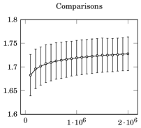
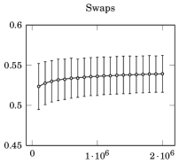
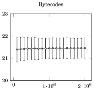
Figure 5: Comparison of sample means with the asymptotics computed in Section 3. The asymptotics are shown as solid lines, the sample means are indicated by circles. Additionally, the error bars show the sample standard deviation. On the $x$-axis, the input size $n$ is shown, the $y$-axis shows the corresponding counts normalized by $n\ln n$.

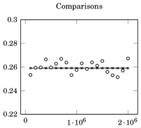
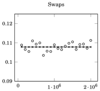
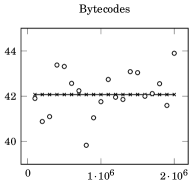
Figure 6: Comparison of sample variances with the asymptotics computed in Section 4. The asymptotics are shown as solid lines, the sample variances are indicated by circles. On the $x$-axis, the input size $n$ is shown, the $y$-axis shows the corresponding variances normalized by $n^{2}$.

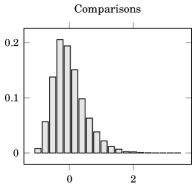
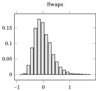
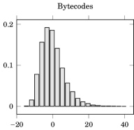
Figure 7: Histograms for the distributions of the normalized number of comparisons $C^{*}{}_{\mkern-13.0mun}\mkern 1.0mu$, swaps $S^{*}{}_{\mkern-13.0mun}\mkern 1.0mu$ and executed Bytecode instructions $\mathit{BC}^{*}{}_{\mkern-13.0mun}\mkern 1.0mu$ from the sample of $10\,000$ random permutations of size $n=10^{6}$.

In this paper, we computed asymptotics for mean and variance of the costs of Yaroslavskiy’s algorithm. Whereas the results for the mean are very precise and indeed can be made exact with some additional diligence, our contraction arguments only provide leading term asymptotics. In this section, we compare the asymptotic approximations with experimental sample means and variances.

We use the Java implementation given in Appendix C and run it on $10\,000$ pseudo-randomly generated permutations of $\{1,\ldots,n\}$ for each of the $20$ sizes in $\{10^{5},\mbox{$2\cdot 10^{5}$},\ldots,\mbox{$2\cdot 10^{6}$}\}$. Note that for sensible estimates of variances, much larger samples are needed than for means. The experiment itself is done using our tool MaLiJAn, which automatically counts the number of comparisons, swaps and Bytecode instructions [Wild et al., 2013].

Figure 5 shows the results for the expected costs and Figure 6 compares asymptotic and sampled variances. The histograms in Figure 7 give some impression how the limit laws will look like.

It is clearly visible in Figure 5 that for the given range of input sizes, the average costs computed in Section 3 are extremely precise. In fact, hardly any deviation between prediction and measurement is visible. The variances in Figure 6 show more erratic behavior. As variances are much harder to estimate than means, this does not come as a surprise. From the data we cannot tell whether the true variances show some oscillatory behavior (in lower order terms) or whether we observe sampling noise. Nevertheless, Figure 6 shows that for the given range of sizes, the asymptotic is a sensible approximation of the exact variance.

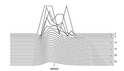
Figure 8: This figure shows the distributions of the normalized number of comparisons $C^{*}{}_{\mkern-13.0mun}\mkern 1.0mu$ for small $n$. The distributions are computed by unfolding the distributional recurrence (D.1). This figure serves as visual evidence for the convergence of cost distributions to a limit law. It is heavily inspired by a corresponding figure for classic Quicksort [Sedgewick and Flajolet, 1996, Figure 1.3].

Figure 8 shows how fast the exact probability distribution of the normalized number of comparisons approaches a smooth limiting shape even for tiny $n$. This strengthens the above quantitative arguments that the limiting distributions computed in this paper are useful approximations of the true behavior of costs in Yaroslavskiy’s algorithm.

References

- Bentley and McIlroy [1993] Jon L. Bentley and M. Douglas McIlroy. Engineering a sort function. Software: Practice and Experience, 23(11):1249–1265, 1993.
- Camesi et al. [2006] Andrea Camesi, Jarle Hulaas, and Walter Binder. Continuous Bytecode Instruction Counting for CPU Consumption Estimation. In Third International Conference on the Quantitative Evaluation of Systems, pages 19–30. IEEE, 2006. ISBN 0-7695-2665-9.
- Chern and Hwang [2001] Hua-Huai Chern and Hsien-Kuei Hwang. Transitional behaviors of the average cost of quicksort with median-of-. Algorithmica, 29(1-2):44–69, 2001.
- Cormen et al. [2009] Thomas H. Cormen, Charles E. Leiserson, Ronald L. Rivest, and Clifford Stein. Introduction to Algorithms. MIT Press, 3rd edition, 2009. ISBN 978-0-262-03384-8.
- David and Nagaraja [2003] Herbert A. David and Haikady N. Nagaraja. Order Statistics. Wiley-Interscience, 3rd edition, 2003. ISBN 0-471-38926-9.
- Dijkstra [1976] Edsger W. Dijkstra. A Discipline of Programming. Prentice Hall PTR, 1st edition, 1976. ISBN 013215871X.
- Durand [2003] Marianne Durand. Asymptotic analysis of an optimized quicksort algorithm. Information Processing Letters, 85(2):73–77, 2003.
- Emden [1970] Maarten H. van Emden. Increasing the efficiency of quicksort. Communications of the ACM, pages 563–567, 1970.
- Fill and Janson [2000] James Allen Fill and Svante Janson. Smoothness and decay properties of the limiting Quicksort density function. In Mathematics and computer science (2000), Trends Math., pages 53–64. Birkhäuser, Basel, 2000.
- Fill and Janson [2002] James Allen Fill and Svante Janson. Quicksort asymptotics. Journal of Algorithms, 44(1):4–28, 2002.
- Graham et al. [1994] Ronald L. Graham, Donald E. Knuth, and Oren Patashnik. Concrete mathematics: a foundation for computer science. Addison-Wesley, 1994. ISBN 978-0-20-155802-9.
- Hennequin [1989] Pascal Hennequin. Combinatorial analysis of Quicksort algorithm. Informatique théorique et applications, 23(3):317–333, 1989.
- Hennequin [1991] Pascal Hennequin. Analyse en moyenne d’algorithmes : tri rapide et arbres de recherche. PhD Thesis, Ecole Politechnique, Palaiseau, 1991.
- Hoare [1961a] Charles Antony Richard Hoare. Algorithm 64: Quicksort. Communications of the ACM, 4(7):321, July 1961a.
- Hoare [1961b] Charles Antony Richard Hoare. Algorithm 63: Partition. Communications of the ACM, 4(7):321, July 1961b.
- Hoare [1962] Charles Antony Richard Hoare. Quicksort. The Computer Journal, 5(1):10–16, January 1962.
- Hwang and Neininger [2002] Hsien-Kuei Hwang and Ralph Neininger. Phase change of limit laws in the quicksort recurrence under varying toll functions. SIAM Journal on Computing, 31(6):1687–1722 (electronic), 2002.
- Kendall [1945] Maurice G. Kendall. The advanced theory of statistics. Charles Griffin, London, 2nd edition, 1945.
- Knuth [1998] Donald E. Knuth. The Art Of Computer Programming: Searching and Sorting. Addison Wesley, 2nd edition, 1998. ISBN 978-0-20-189685-5.
- Knuth [2005] Donald E. Knuth. The Art of Computer Programming: Volume 1, Fascicle 1. MMIX, A RISC Computer for the New Millennium. Addison-Wesley, 2005. ISBN 0-201-85392-2.
- Kushagra et al. [2014] Shrinu Kushagra, Alejandro López-Ortiz, Aurick Qiao, and J. Ian Munro. Multi-Pivot Quicksort: Theory and Experiments. In ALENEX 2014, pages 47–60. SIAM, 2014.
- Laube and Nebel [2010] Ulrich Laube and Markus E. Nebel. Maximum likelihood analysis of algorithms and data structures. Theoretical Computer Science, 411(1):188–212, January 2010.
- Lindholm and Yellin [1999] Tim Lindholm and Frank Yellin. Java Virtual Machine Specification. Addison-Wesley Longman Publishing, 2nd edition, April 1999. ISBN 0-201-43294-3.
- Mahmoud [2000] Hosam M. Mahmoud. Sorting: A distribution theory. John Wiley & Sons, 2000. ISBN 1-118-03288-8.
- Martínez and Roura [2001] Conrado Martínez and Salvador Roura. Optimal Sampling Strategies in Quicksort and Quickselect. SIAM Journal on Computing, 31(3):683, 2001.
- McDiarmid [1998] Colin McDiarmid. Concentration. In Probabilistic methods for algorithmic discrete mathematics, pages 195–248. Springer, 1998.
- McDiarmid and Hayward [1996] Colin McDiarmid and Ryan B. Hayward. Large deviations for Quicksort. Journal of Algorithms, 21(3):476–507, 1996.
- McMaster [1978] Colin L. McMaster. An analysis of algorithms for the Dutch National Flag Problem. Communications of the ACM, 21(10):842–846, October 1978.
- Nebel and Wild [2014] Markus E. Nebel and Sebastian Wild. Pivot Sampling in Dual-Pivot Quicksort. In International Conference on Probabilistic, Combinatorial and Asymptotic Methods for the Analysis of Algorithms 2014, 2014. URL http://arxiv.org/abs/1403.6602.
- Neininger [2001] Ralph Neininger. On a multivariate contraction method for random recursive structures with applications to Quicksort. Random Structures & Algorithms, 19(3-4):498–524, 2001.
- Regnier [1989] Mireille Regnier. A limiting distribution for Quicksort. Informatique théorique et applications, 23(3):335–343, 1989.
- Rösler [1991] Uwe Rösler. A limit theorem for “quicksort”. Informatique théorique et applications, 25(1):85–100, 1991.
- Rösler [2001] Uwe Rösler. On the analysis of stochastic divide and conquer algorithms. Algorithmica, 29(1):238–261, 2001.
- Sedgewick [1975] Robert Sedgewick. Quicksort. PhD Thesis, Stanford University, 1975.
- Sedgewick [1977] Robert Sedgewick. The analysis of Quicksort programs. Acta Informatica, 7(4):327–355, 1977.
- Sedgewick and Flajolet [1996] Robert Sedgewick and Philippe Flajolet. An Introduction to the Analysis of Algorithms. Addison-Wesley-Longman, 1996. ISBN 978-0-201-40009-0.
- Singleton [1969] Richard C. Singleton. Algorithm 347: an efficient algorithm for sorting with minimal storage [M1]. Communications of the ACM, 12(3):185–186, March 1969.
- Tan and Hadjicostas [1995] Kok Hooi Tan and Petros Hadjicostas. Some properties of a limiting distribution in Quicksort. Statistics & Probability Letters, 25(1):87–94, October 1995.
- Wild [2012] Sebastian Wild. Java 7’s Dual Pivot Quicksort. Master thesis, University of Kaiserslautern, 2012.
- Wild and Nebel [2012] Sebastian Wild and Markus E. Nebel. Average Case Analysis of Java 7’s Dual Pivot Quicksort. In Leah Epstein and Paolo Ferragina, editors, European Symposium on Algorithms 2012, volume 7501 of LNCS, pages 825–836. Springer, 2012.
- Wild et al. [2013] Sebastian Wild, Markus E. Nebel, Raphael Reitzig, and Ulrich Laube. Engineering Java 7’s Dual Pivot Quicksort Using MaLiJAn. In Meeting on Algorithm Engineering and Experiments 2013, pages 55–69, 2013.