Computational study of subcritical response in flow past a circular cylinder

Abstract

Flow past a circular cylinder is investigated in the subcritical regime, below the onset of Bénard-von Kármán vortex shedding at $\mathrm{Re}_{c}\simeq 47$. The transient response of infinitesimal perturbations is computed. The domain requirements for obtaining converged results is discussed at length. It is shown that energy amplification occurs as low as $\mathrm{Re}=2.2$. Throughout much of the subcritical regime the maximum energy amplification increases approximately exponentially in the square of $\mathrm{Re}$ reaching $6800$ at $\mathrm{Re}_{c}$. The spatiotemporal structure of the optimal transient dynamics is shown to be transitory Bénard-von Kármán vortex streets. At $\mathrm{Re}\simeq 42$ the long-time structure switches from exponentially increasing downstream to exponentially decaying downstream. Three-dimensional computations show that two-dimensional structures dominate the energy growth except at short times.

I Introduction

Incompressible fluid flow past a circular cylinder has been extensively studied, both for its relevance to numerous engineering applications and as a prototype bluff-body flow exhibiting vortex shedding. See for example Zdravkovich (1997, 2003) and references therein. It is one of the most-used test bed for exploring stability concepts in open flows, e.g. Provansal et al. (1987); Jackson (1987); Zebib (1987); Yang and Zebib (1989); Dušek et al. (1994); Noack and Eckelmann (1994); Pier (2002); Noack et al. (2003); Chomaz (2005); Barkley (2006); Giannetti and Luchini (2007). As a result, a great deal is known about this flow in general and in particular concerning the primary instability. It is well-established that this instability occurs at a critical Reynolds number of about 47 Provansal et al. (1987); Jackson (1987); Zebib (1987). Below this value the steady wake flow is linearly stable, while above it the steady flow is unstable and periodic oscillations arise leading to the famous Bénard-von Kármán vortex street Bénard (1908); von Kármán (1911). Our concern here is what happens in the stable, subcritical regime prior to, and leading up to, the onset of oscillations.

Stable flows may exhibit transient growth Schmid and Henningson (2001); Trefethen and Embree (2005). This means that infinitesimal perturbations to the flow may grow in energy for some time before subsequently decaying to zero. While initially popular in parallel shear flows as possibly playing a role in the transition to turbulence, e.g. Gustavsson (1991); Butler and Farrell (1992); Henningson et al. (1993), transient growth has become increasingly of interest in spatially developing flows, e.g. Cossu and Chomaz (1997); Chomaz (2005); Åkervik et al. (2007); Blackburn et al. (2008a); Marquet et al. (2008a); Alizard et al. (2009). For instance, separated flows arising due to abrupt changes in geometry are known to promote extremely large transient growth in perturbations Blackburn et al. (2008a, b); Cantwell et al. (2010). The origin of this growth can be traced to the non-normality of the linear stability operator associated with many shear flows Chomaz (2005); Schmid and Henningson (2001). This means, in particular, that in spatially developing flows the eigenmodes of the stability operator tend to be located downstream while the eigenmodes of the adjoint operator tend to be located upstream Trefethen and Embree (2005); Chomaz (2005); Giannetti and Luchini (2007).

For the cylinder wake, Giannetti and Luchini Giannetti and Luchini (2007) first examined in detail the adjoint eigenmodes in the vicinity of the primary instability and used these, together with direct eigenmodes, to understand the sensitivity of the flow. Their results are further discussed in detail by Chomaz in the context of non-normality Chomaz (2005). Since this important work, there have been further computations of direct and adjoint modes and transient growth for the cylinder wake. For example Marquet et al. Marquet et al. (2008b) have computed direct and adjoint eigenmodes of the supercritical flow, and Abdessemed et al. Abdessemed et al. (2009) have studied the transient growth, focusing on supercritical Reynolds numbers, although also reporting some subcritical values.

There have been a number of experimental studies of the cylinder wake in the stable and marginally unstable regime Provansal et al. (1987); Le Gal and Croquette (2000); Marais et al. (2010). The most relevant are the studies by Le Gal and Croquette Le Gal and Croquette (2000) and the recent work by Marais et al. Marais et al. (2010) on the impulse response at subcritical Reynolds numbers. By inducing an impulse through a small displacement or rotation of the cylinder, wavepackets are generated that grow and are subsequently advected downstream. While the measurements by Le Gal and Croquette provide informative qualitative properties of the transient dynamics, these measurements were made using streaklines and so provide limited quantitative detail. The more recent work by Marais et al. uses particle image velocimetry to obtain quantitative measurements of the transient response in the subcritical regime.

The purpose of the current study is two-fold. Primarily we establish an accurate characterization of the optimal transient energy growth throughout the subcritical regime for the cylinder wake. We determine the threshold Reynolds number where energy growth first occurs, determine the Reynolds number dependence of the optimal growth, and its value at criticality. We show that the transient dynamics associated with optimal energy growth is in the form of wave packets similar to those observed in experiments on subcritical wakes. The secondary purpose of the paper is to highlight and establish the computational requirements for such computations. As we shall show, the requirements for accurate computations of transient growth are more severe than those of linear stability. While these findings are specific to the cylinder wake, they should guide computations of similar flows.

II Formulation

The flow geometry is illustrated in Fig. 1. A circular cylinder of diameter $D$ is placed in a free-stream flow $U_{\infty}\bm{e_{x}}$. Streamwise $x$ and cross-stream $y$ coordinates are centered on the circular cross section. The cylinder axis, infinite in length and normal to the free-stream velocity, aligns with the $z$-coordinate.

In principle this open flow would have infinite extent in all directions. In practice, however, our numerical calculations necessarily employ a computational domain $\Omega$ with finite inflow $L_{i}$, outflow $L_{o}$, and cross-stream $L_{c}$ lengths, as illustrated. The $z$-direction is homogeneous, and for the issues addressed in this paper, this direction can be treated without needing to restrict to a bounded domain. The demands on the domain dimensions is an important aspect of our work discussed in detail in Sec. III.

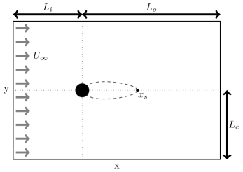
Figure 1: Diagram of the cylinder geometry (not to scale), showing the inflow, outflow and cross-stream dimensions referenced later. Also marked are the separation streamlines and the downstream stagnation point, $x_{s}$.

The fluid is governed by the incompressible Navier-Stokes equations

$$\partial_{t}\mathbf{u}+(\mathbf{u}\cdot\nabla)\mathbf{u} =-\nabla p+\mathrm{Re}^{-1}\nabla^{2}\mathbf{u},$$ (1a)

$$\nabla\cdot\mathbf{u} =0,$$ (1b)

where $\mathbf{u}=\mathbf{u}(\mathbf{x})=(u(x,y,z),v(x,y,z),w(x,y,z))$ is the fluid velocity and $p(x,y,z)$ is the static pressure. Without loss of generality we set the density to unity. The equations are non-dimensionalized by the free-stream speed $U_{\infty}$ and the cylinder diameter $D$. The Reynolds number $\mathrm{Re}$ is therefore given as

$$\mathrm{Re}=\frac{U_{\infty}D}{\nu},$$

where $\nu$ is the kinematic viscosity of the fluid.

No-slip boundary conditions are imposed on the cylinder surface. The boundary conditions around the outer boundaries of the domain are such as to give a good numerical approximation of the unbounded flow. Specifically, the boundary conditions are:

$$\bm{u}(\partial\Omega_{i},t) =U_{\infty}\bm{e_{x}},$$ (2a)

$$\bm{u}(\partial\Omega_{c},t) =U_{\infty}\bm{e_{x}},$$ (2b)

$$\bm{u}(\partial\Omega_{w},t) =\bm{0},$$ (2c)

$$\partial_{x}\bm{u}(\partial\Omega_{o},t) =0,\quad p(\partial\Omega_{o},t)=0,$$ (2d)

where $\partial\Omega_{i}$ is the inlet boundary at $x=-L_{i}$, $\partial\Omega_{c}$ is the cross-stream boundary at $y=\pm L_{c}$, $\partial\Omega_{w}$ is the boundary of the cylinder, and $\partial\Omega_{o}$ is the outlet boundary at $x=L_{o}$.

The remaining material in this section is included for completeness and to clearly define notation. Since the details are contained in numerous prior publications, especially Tuckerman and Barkley (2000); Barkley et al. (2008), the treatment here is minimal.

Equation (1) is solved using Direct Numerical Simulation (DNS) employing a split-step pressure-correction scheme described elsewhere Orszag et al. (1986); Karniadakis et al. (1991). This is implemented in a spectral-element code Blackburn and Sherwin (2004) utilizing an elemental decomposition of the domain in the two-dimensional (2D) plane normal to the cylinder axis.

The base flows $\mathbf{U}$ considered in this paper are steady, two-dimensional solutions to Eq. (1). Hence $\mathbf{U}=(U(x,y),V(x,y))$. These Reynolds number dependent flows are symmetric about the streamwise centerline as depicted in Fig. 1. Figure 2 shows a typical base flow. Those at other $\mathrm{Re}$ are qualitatively similar, differing primarily in the length of the recirculation region behind the cylinder. For $\mathrm{Re}\lesssim 6.2$, there is no recirculation region. Steady base flows in both subcritical and supercritical regimes are rapidly obtained through DNS by imposing this midplane symmetry. Once computed, base flows are stored for use in subsequent linear calculations.

Figure 2: Representative base flow. Streamlines of the flow at $\mathrm{Re}$=40. The computational domain is much larger than the region shown. The main flow field uses a contour spacing of 0.25, while a smaller spacing of 0.01 is used to highlight the structure of the recirculation bubble.

Our interest is in the dynamics of infinitesimal perturbations $\mathbf{u^{\prime}}$ to the steady base flow. These perturbations evolve according to the linearized Navier-Stokes equations

$$\partial_{t}\mathbf{u^{\prime}}+(\mathbf{u^{\prime}}\cdot\nabla)\mathbf{U}+(\mathbf{U}\cdot\nabla)\mathbf{u^{\prime}} =-\nabla p^{\prime}+\mathrm{Re}^{-1}\nabla^{2}\mathbf{u^{\prime}},$$ (3a)

$$\nabla\cdot\mathbf{u^{\prime}} =0,$$ (3b)

where $p^{\prime}$ is the perturbation pressure. Numerically Eq. (3) is solved using the same techniques as the nonlinear Navier-Stokes equations. For the most part we will focus on 2D perturbation fields $\mathbf{u^{\prime}}=(u^{\prime},v^{\prime})$ on 2D grids. However, we will also consider briefly three-dimensional perturbations. Since the base flow is 2D, three-dimensional (3D) perturbations can be decomposed into non-interacting modes of the form

$$\mathbf{u^{\prime}}(x,y,z)=\mathbf{\hat{u}}(x,y)e^{i\beta z}+c.c.,$$ (4)

where $\beta$ is the spanwise wavenumber of the perturbation. Only $\mathbf{\hat{u}}(x,y)$, a three-component field on a two-dimensional grid, needs to be computed.

Our primary focus is on the transient dynamics of perturbations at subcritical Reynolds numbers. We focus on the energy of perturbation fields and seek initial conditions $\mathbf{u^{\prime}}(0)$ which generate the largest possible growth in energy under evolution by Eq. (3). The formalism is as follows. Let $\mathcal{A}(\tau)$ denote the linear evolution operator over a time $\tau$  defined by Eq. (3), so that

$$\mathbf{u^{\prime}}(\tau)=\mathcal{A}(\tau)\mathbf{u^{\prime}}(0).$$

Since the governing equations are linear it is sufficient to consider initial perturbation fields with $||\mathbf{u^{\prime}}(0)||^{2}=\langle\mathbf{u^{\prime}}(0),\mathbf{u^{\prime}}(0)\rangle=1$, where $\langle\cdot,\cdot\rangle$ denotes the $L_{2}$ inner-product. Then the energy growth in the perturbation field over a time $\tau$ is given by

$$\frac{E(\tau)}{E(0)}=\langle\mathbf{u^{\prime}}(\tau),\mathbf{u^{\prime}}(\tau)\rangle.$$

In terms of the operator $\mathcal{A}(\tau)$, and its adjoint $\mathcal{A}^{\ast}(\tau)$ in the $L_{2}$ inner-product, we have

$$\frac{E(\tau)}{E(0)}= \langle\mathcal{A}(\tau)\mathbf{u^{\prime}}(0),\mathcal{A}(\tau)\mathbf{u^{\prime}}(0)\rangle$$

$$= \langle\mathbf{u^{\prime}}(0),\mathcal{A}^{\ast}(\tau)\mathcal{A}(\tau)\mathbf{u^{\prime}}(0)\rangle.$$

Letting $\lambda_{j}$ and $\mathbf{v}_{j}$ denote eigenvalues and normalized eigenfunctions of the operator $\mathcal{A}^{\ast}(\tau)\mathcal{A}(\tau)$, we have

$$\mathcal{A}^{\ast}(\tau)\mathcal{A}(\tau)\mathbf{v}_{j}=\lambda_{j}\mathbf{v}_{j},\qquad||\mathbf{v}_{j}||=1.$$ (5)

The eigenvalues are non-negative and we assume ordering $\lambda_{1}\geq\lambda_{2}\geq\cdots$.

The maximum possible energy growth, denoted $G(\tau)$, over a specified time horizon $\tau$, is then given by the dominant eigenvalue of $\mathcal{A}^{\ast}(\tau)\mathcal{A}(\tau)$, i.e.

$$G(\tau)=\max_{j}\lambda_{j}=\lambda_{1},$$

The initial perturbation leading to this growth is the corresponding eigenfunction $\mathbf{v}_{1}$. While the dominant eigenvalue of $\mathcal{A}^{\ast}(\tau)\mathcal{A}(\tau)$ is generally of most importance, the first few sub-dominant eigenvalues may also be of interest. In particular $\mathbf{v}_{2}$ will also be considered in this study.

The maximum energy growth over all time horizons is denoted by

$$G^{\max}=G(\tau^{\max}),$$ (6)

where

$$\tau^{\max}=\operatorname*{arg\,max}_{\tau}G(\tau).$$ (7)

While our primary focus is transient growth, we report some eigenvalue results. Equation (3) can formally be written

$$\partial_{t}{\mathbf{u^{\prime}}}=\mathcal{L}\mathbf{u^{\prime}},$$

Looking for normal-mode solutions to these equations gives the eigenvalue problem

$$\mathcal{L}\tilde{\bm{u}}_{j}=\sigma_{j}\tilde{\bm{u}}_{j},\qquad||\tilde{\bm{u}}_{j}||=1,$$ (8)

where $\tilde{\bm{u}}_{j}$ are normalized eigenmodes and $\sigma_{j}$ eigenvalues of $\mathcal{L}$. We assume ordering such that ${\rm Re}(\sigma_{1})\geq{\rm Re}(\sigma_{2})\geq\cdots$. Stability of the base flow is determined from the right-most eigenvalues of $\mathcal{L}$ in the complex plane.

Associated to Eq. (8) is the adjoint eigenvalue problem

$$\mathcal{L}^{*}\bm{u}^{*}_{j}=\sigma_{j}^{*}\bm{u}^{*}_{j},$$ (9)

where $\bm{u}^{*}_{j}$ are the adjoint modes, (eigenmodes of the adjoint operator $\mathcal{L}^{*}$), and $\sigma_{j}^{*}$ is the complex conjugate of $\sigma_{j}$. The norm of the adjoint eigenmodes is chosen so that $\langle\bm{u}^{*}_{j},\tilde{\bm{u}}_{j}\rangle=1$ for all $j$. Then the eigenmode and adjoint modes satisfy biorthonormality:

$$\langle\bm{u}^{*}_{i},\tilde{\bm{u}}_{j}\rangle=\delta_{ij}.$$

In practice the eigenvalues for the transient growth or stability problems are computed through a modified Arnoldi algorithm using a time-stepper approach Tuckerman and Barkley (2000); Barkley et al. (2008).

III Influence of Domain Size

As noted in the introduction, the size of the computational domain can be an important factor in studies of the transient response in subcritical cylinder flow. While the requirements for accurate base flows and eigenvalue calculations for the cylinder wake have been discussed in many places Fornberg (1980); Lecointe and Piquet (1984); Strykowski and Hannemann (1991); Anagnostopoulos et al. (1998), and are presented in our study in the Appendix, there is no such discussion for transient growth calculations for the cylinder wake. Hence some details are worthwhile. We first present results from the convergence study and then discuss some of the causes and implications of our findings.

III.1 Convergence

We focus on the role of inflow length, $L_{i}$, and the cross-stream half-length, $L_{c}$, since these are the critical lengths. The requirements on the outflow length, $L_{o}$, are set by the largest $\tau$ value under consideration in the transient growth analysis and could in principle be arbitrarily large. Based on the maximum value of $\tau=110$ we consider, and a free-stream $U_{\infty}=1$, we fix the outflow length in the convergence study at $L_{o}=125$.

Figure 3 shows a representative spectral-element domain of the type used in our computations. (It is in fact the final mesh used for obtaining results presented in Sec. IV.) For the study of domain size, $L_{i}$ and $L_{c}$ are varied by adding or removing elements as necessary, and the polynomial order of the spectral expansion within each element is fixed at order 8. The polynomial order used in obtaining the final transient growth results is $6$, as established in the Appendix.

Figure 3: Representative spectral-elemental mesh. Dimensions are $L_{i}=45$, $L_{c}=45$ and $L_{o}=125$ (refer to Fig. 1 for definitions).

The dependence of these calculations on domain size is assessed through the calculation of energy growth at a fixed time horizon of $\tau=20$. At this time horizon non-negligible growth is expected across most of the range of Reynolds numbers under consideration. Figure 4 summarizes the errors introduced through domain size restriction. Three Reynolds numbers, $\mathrm{Re}=5$, $\mathrm{Re}=20$ and $\mathrm{Re}=46$, are considered to ensure that the mesh is capable of resolving all solutions in the subcritical range.

The transient growth results are seen to be sensitive to domain size, much more so than either the base flow or eigenvalue calculations presented in the appendix. Domains that provide results accurate to within 1% for base flows and eigenvalues, e.g. a domain with $L_{i}=L_{c}=25$, do not provide such accuracy for transient growth calculations. The effect of cross-stream restriction at low $\mathrm{Re}$ is particularly significant. Even accepting that in many cases one does not need high accuracy in transient growth values, Fig. 4 demonstrates the care that must be taken in computing transient response in the subcritical regime.

Based on these results, a computational domain with $L_{i}=45$ and $L_{c}=45$ is deemed sufficient to resolve transient growth calculations to within about 1% for subcritical Reynolds numbers. Possibly the accuracy is not quite 1% at $\mathrm{Re}<5$, but the growth values are sufficient for our purposes. A diagram of the resulting mesh is shown in Fig. 3.

Figure 4: Convergence of optimal growth calculation with mesh geometry by (a) in-flow length $L_{i}$ and (b) cross-stream length $L_{c}$. Points indicate the computed values. Optimal growth is for a time horizon of $\tau=20$. Percentage errors are shown relative to the calculation using $L_{i}=65$ and $L_{c}=65$, respectively.

III.2 Discussion

We begin by recalling that recently, Abdessemed et al. Abdessemed et al. (2009) reported transient growth calculations in the cylinder wake, including some within the subcritical regime at $\mathrm{Re}=45$. In comparing those results with ours, we have found that their growth values are about 32% larger than those computed on the mesh in Fig. 3, at the same $\mathrm{Re}$ and time horizon. We will use this discrepancy to focus the present discussion.

The Abdessemed et al. calculations were performed using a spectral-element code similar to that used in this study. Their computational domain has bounds $-8\leq x\leq 95$ and $-12.5\leq y\leq 12.5$ and identical boundary conditions to ours. One can quickly rule out the possibility that resolution (polynomial order) or outflow length are significant factors in the disagreement between the two computations. Moreover, we have already seen that the transient growth calculations require large inflow $L_{i}$ and cross-stream $L_{c}$ dimensions so the disagreement is not surprising in retrospect. However, there are in fact two causes for the discrepancy which we address: one is the indirect effect caused by differences in the base flows for the different computations and the other is the direct effect of domain requirements for the optimal initial condition itself.

We shall refer to our computational domain with dimensions as in Fig. 3 as $\Omega_{\text{L}}$, (large domain), and that with dimensions used by Abdessemed et al. as $\Omega_{\text{S}}$, (small domain). Let $\mathbf{U}_{\text{L}}$ denote the base flow computed on $\Omega_{\text{L}}$ (at $\mathrm{Re}=45$) and let $\mathbf{u^{\prime}}_{\text{L}}$ denote the normalized initial condition, $||\mathbf{u^{\prime}}_{\text{L}}||=1$, giving optimal growth at $\tau=100$. Similarly let $\mathbf{U}_{\text{S}}$ and $\mathbf{u^{\prime}}_{\text{S}}$ denote the base flow and normalized optimal initial condition on $\Omega_{\text{S}}$. The resulting energy growth for the two calculations is given in the first two rows of Table 1, where one sees the large discrepancy. It is worth pointing out that the critical Reynolds numbers obtained on the two meshes differ by only about 2%.

To assess the role of the base flow, one can take the initial condition $\mathbf{u^{\prime}}_{\text{S}}$ from the smaller domain and evolve it on the larger domain with the corresponding base flow $\mathbf{U}_{\text{L}}$. The resulting growth after 100 time units is given in the third row of Table 1. Necessarily the growth had to be less than for $\mathbf{u^{\prime}}_{\text{L}}$ because $\mathbf{u^{\prime}}_{\text{L}}$, by definition, gives the largest possible growth over this time horizon on $\Omega_{\text{L}}$. It is perhaps somewhat surprising, however, that the growth following from the fixed initial condition $\mathbf{u^{\prime}}_{\text{S}}$ is approximately factor of 2 less on the large domain than on the small domain (second and third rows of Table 1). The difference is almost entirely attributable to the difference in the base flows $\mathbf{U}_{\text{L}}$ and $\mathbf{U}_{\text{S}}$. This is confirmed by evolving $\mathbf{u^{\prime}}_{\text{S}}$ on the small domain but with the base flow $\mathbf{U}_{\text{L}}$, truncated onto the smaller domain. The result is given in the last row of Table 1. There is little difference between the evolution of $\mathbf{u^{\prime}}_{\text{S}}$ on the two domains, if they both have the same base flow $\mathbf{U}_{\text{L}}$. The conclusion is that the energy growth may depend considerably on the base flow (a factor of 2 in this case), even in situations where other measures, such as critical Reynolds numbers, would not reveal such a large dependency.

There is then the remaining issue of how $\mathbf{u^{\prime}}_{\text{L}}$ and $\mathbf{u^{\prime}}_{\text{S}}$ differ and why the energy growth following from $\mathbf{u^{\prime}}_{\text{S}}$ is 27% less than from $\mathbf{u^{\prime}}_{\text{L}}$ for the same base flow (first and third rows in Table 1). This has to do with the domain requirements, in particular the inflow length $L_{i}$ needed to capture the optimal initial condition. In Fig. 5 we show the upstream extent of $\mathbf{u^{\prime}}_{\text{L}}$ on two scales. The energy of the perturbation upstream of $x=-5$ is of the order $10^{-5}$ and, while one might consider it to be negligible, this portion of the initial condition makes a significant contribution to the overall growth and cannot be neglected in the transient growth computations if quantitative accuracy is required.

We conclude with a few further remarks on the presence of weak upstream tails in the optimal initial conditions. First, despite our caution about the need to resolve these to obtain quantitatively accurate results, we find the linear evolution from the optimal initial condition is qualitatively similar whether or not the numerical domain fully contains the weak upstream tail of the initial condition. We observe no important qualitative errors in discounting it, but quantitatively the errors in the energy growth can be large. In addition, the length of the upstream tail depends on the time horizon $\tau$. The value $\tau$=100 considered in our comparison is rather large. For smaller time horizons the weak tail may be absent from the optimal initial condition simply because such a tail could not advect downstream and come into play over a small time horizon. Specifically, in Sec. IV.2 we focus on optimal initial conditions computed for $\tau$=20 and in this case the upstream tails are absent.

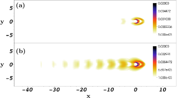
Figure 5: (color online) Energy of the optimal initial condition for $\mathrm{Re}=45$, $\tau=100$ shown on two scales: (a) matching that of the figures shown later in the paper and, (b) showing an extended scale which highlights the upstream tail of the perturbation.

domain	base flow	IC	$E(100)$
$\Omega_{\text{L}}$	$\mathbf{U}_{\text{L}}$	$\mathbf{u^{\prime}}_{\text{L}}$	$2.54\times 10^{3}$
$\Omega_{\text{S}}$	$\mathbf{U}_{\text{S}}$	$\mathbf{u^{\prime}}_{\text{S}}$	$3.36\times 10^{3}$
$\Omega_{\text{L}}$	$\mathbf{U}_{\text{L}}$	$\mathbf{u^{\prime}}_{\text{S}}$	$1.85\times 10^{3}$
$\Omega_{\text{S}}$	$\mathbf{U}_{\text{L}}$	$\mathbf{u^{\prime}}_{\text{S}}$	$1.77\times 10^{3}$

Table 1: Effects of domain size, base flow, and initial condition (IC) on the energy growth at $\mathrm{Re}=45$. Energy at time $100$ is given for different configurations (see text).

IV Transient Subcritial Response

IV.1 2D Energy Growth

Figures 6 and 7 summarize the optimal energy growth for 2D perturbations in the subcritical regime. Figure 6 shows the optimal growth envelopes for particular values of $\mathrm{Re}$. To be clear, these curves show the largest attainable energy growth over all possible initial conditions at each value of $\tau$. The uppermost curve is the growth at $Re=50$, above the onset of linear instability at $\mathrm{Re}_{c}$. After an initial rapid growth, the energy increase saturates to an exponential rate, in line with that of the leading eigenvalue.

Figure 7 shows growth contours in the ($\mathrm{Re}$, $\tau$) plane. The contours highlight the fast energy growth at small time horizons and the slow decay for long $\tau$. The thick curve denotes the no-growth contour: $G=1$. The interception of this curve with the $\mathrm{Re}$-axis indicates a critical Reynolds number for energy growth Joseph (1976), $\mathrm{Re}_{E}$, below which all perturbations decay monotonically in time and above which there is transient energy growth for at least some perturbations. We estimate $\mathrm{Re}_{E}=2.2$. Thus, a small amount of transient energy growth is possible before the formation of the recirculation region behind the cylinder at $\mathrm{Re}=6.2$.

Figure 6: Optimal energy growth at Reynolds numbers from $\mathrm{Re}=5$ to $\mathrm{Re}=50$ in increments of $\mathrm{Re}=5$. Points indicate the computed values. The case $\mathrm{Re}=50$ is above $\mathrm{Re}_{c}$ and is shown as dashed. The horizontal line is an estimate of the maximum growth in the subcritical regime (see text).

Figure 7: Contour plot of optimal energy growth in the subcritical regime, with contour levels as indicated. The thick black curve denotes the contour of no-growth, $G=1$.

The single most important measure of the transient energy growth at any $\mathrm{Re}$ is the maximum $G^{\max}$ over all $\tau$. [Recall Eqs. (6) and (7)]. This is shown in Fig. 8 where $\log_{10}G^{\max}$ is plotted as a function of $\mathrm{Re}^{2}$. Throughout most of the subcritical regime, the maximum growth increases exponentially with $\mathrm{Re}^{2}$. More specifically, we find

$$G^{\max}\simeq\exp(1.55\times 10^{-3}\mathrm{Re}^{2}).$$ (10)

Only for $\mathrm{Re}\gtrsim 40$ does the growth deviate significantly from this form. There is an upturn in the maximum growth in approaching $\mathrm{Re}_{c}$. Above $\mathrm{Re}_{c}$, $G^{\max}=\infty$ since the flow is linearly unstable and $G(\tau)$ diverges as $\tau\to\infty$.

Data up to $\mathrm{Re}=46$ have been obtained via the transient growth calculations described in Sec. II. The maximum growth at $\mathrm{Re}_{c}$ is obtained differently. At criticality, the optimal initial condition is the adjoint eigenmode corresponding to the critical eigenvalue. Under linear evolution, this initial condition evolves to the direct eigenmode. Hence the optimal growth at criticality is obtained from the eigenmode and its adjoint. Taking $||\tilde{u}||=1$ and $\langle u^{*},\tilde{u}\rangle=1$, i.e. biorthonormalized modes, then the maximum growth is given by $||u^{*}||$. Based on these calculations our estimate of the maximum growth at $\mathrm{Re}_{c}$, and hence the maximum growth within the subcritical regime, is $G^{\max}_{c}\equiv G^{\max}(\mathrm{Re}_{c})\approx 6800$.

Figure 8: Maximum growth $G^{max}$ as a function of the square of Reynolds number. The vertical dotted line corresponds to $\mathrm{Re}_{c}$. $G^{max}_{c}$, the maximum growth at $\mathrm{Re}_{c}$, is indicated with a point and is computed differently from cases $\mathrm{Re}\leq 46$ (see text). The dashed-dotted line highlights the relationship given by Eq. (10).

IV.2 Spatiotemporal Evolution

We now turn to one of our primary focuses, the transient evolution of infinitesimal perturbations. For the most part we shall be interested in the qualitative character of this evolution and how it depends on $\mathrm{Re}$.

We start the perturbation field $\mathbf{u^{\prime}}$ from initial conditions calculated for optimal linear energy growth and evolve the field via the linearized Navier-Stokes equations, Eq. (3). Recall from Sec. II that the initial condition giving optimal growth over time horizon $\tau$ is the dominant eigenfunction $\mathbf{v}_{1}$ of $\mathcal{A}^{\ast}(\tau)\mathcal{A}(\tau)$. Hence, the initial condition and subsequent evolution $\mathbf{u^{\prime}}(t)$, depend on time horizon $\tau$ in defining $\mathcal{A}^{\ast}(\tau)\mathcal{A}(\tau)$. However, the transient dynamics based on a substantial range of $\tau$ values are qualitatively very similar. This is illustrated, in part, by Fig. 9 where we show the the optimal growth envelope (denoted by circles) at $\mathrm{Re}=40$ and also the energy evolution from optimal initial conditions corresponding to three quite different values of $\tau$. While there are quantitative differences between the transient-response curves, qualitatively they are similar, suggesting similar flow features and dynamics are excited by initial conditions optimized across a large range of $\tau$ values. This holds for other values of $\mathrm{Re}$, with the peak in the response curves shifting to smaller times for smaller values of $\mathrm{Re}$. In the spatiotemporal results which follow, we have opted to fix the $\tau$ at which the optimal perturbations are computed, rather than having it vary with $\mathrm{Re}$. All optimal perturbations are for $\tau$=20, as this provides a good choice over the whole of the subcritical regime.

Figure 9: Energy of evolving perturbations computed at $\mathrm{Re}$=40 for three time horizons: $\tau$=20, $\tau$=65, and $\tau$=95. The three curves touch the optimal growth envelope (circles) at their respective $\tau$ values. Qualitatively similar evolution is seen over a large range of optimal perturbations.

Visualizations of the linear time evolution of perturbations $\mathbf{u^{\prime}}(t)$, at $\mathrm{Re}$=20 and $\mathrm{Re}$=40 are shown in Figs. 10 and 11. Perturbation energy, $|\mathbf{u^{\prime}}|^{2}/2$ is plotted in Fig. 10 with a fixed energy scale throughout the figure. Figure 11 shows the same evolution, except in terms of vorticity. Here we visualize not the vorticity in the perturbation field itself, but in a superposition of the base flow and the perturbation, i.e. $\mathbf{u}=\mathbf{U}+\epsilon\mathbf{u^{\prime}}$, where $\epsilon$ is chosen so that the resulting superposition best resembles what one might find in an actual flow, as for example, might be observed in experiments. In all cases only a portion of the full computational domain is shown.

The bottom-most plots correspond to the optimal initial conditions $\mathbf{u^{\prime}}(t=0)=\mathbf{v}_{1}$. One can see in the energy plot that the initial condition is more localized to the cylinder at higher $\mathrm{Re}$. In fact the initial condition becomes quite broad spatially at low $\mathrm{Re}$. In the vorticity plot one can see the asymmetry of the combined flow introduced by the perturbation. The base flow $\mathbf{U}$ is symmetric about the centerline, while the perturbation $\mathbf{u^{\prime}}(0)$ is antisymmetric. Note, for the $\mathrm{Re}$ and $\tau$ values considered here, there is no weak upstream tail in the initial conditions of the type shown in Fig. 5(b), although weak upstream tails are found at $\mathrm{Re}$=40 for larger values of $\tau$. These tails play no qualitative role in the spatiotemporal dynamics.

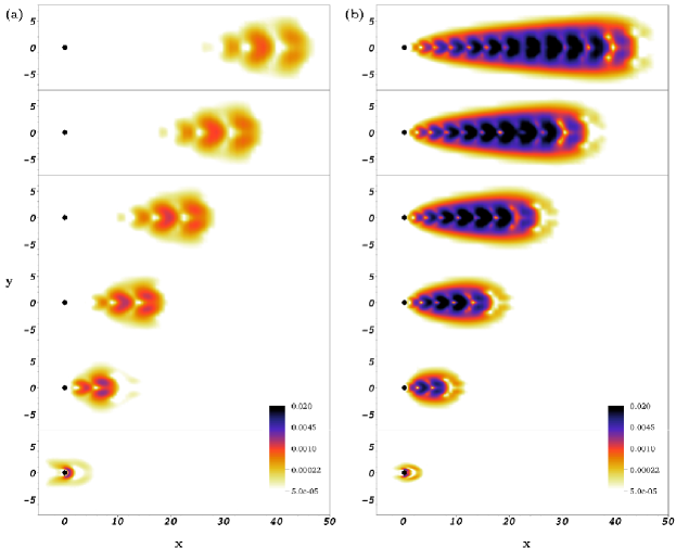
Figure 10: (color online). Contours of energy showing the linear evolution of perturbations at $\mathrm{Re}$=20 (left) and $\mathrm{Re}$=40 (right). The panels are snapshots at 10 time-unit intervals from $t=0$ (bottom) to $t=50$ (top).

The perturbation fields are evolved via the linearized Navier-Stokes equations, Eq. (3), and visualized every 10 time units. The first obvious point is that in both cases the perturbation fields, or more accurately the superposition of the perturbation fields and base flow, resemble transitory Bénard-von Kármán vortex streets. At $\mathrm{Re}=20$, the initial perturbation develops into a packet of roughly two wavelengths in streamwise extent and advects steadily downstream at a speed slightly less than 1. The peak energy is reached at $t\simeq 27$ and thereafter the energy decays quite gradually. At $\mathrm{Re}$=40, the leading edge of the packet, and the streamwise location of the maximum of the response, advects downstream at approximately the same speed as at $\mathrm{Re}$=20. In this case however, the evolving perturbation develops a long trailing series of sinuous oscillations as the excited near-wake region undergoes slowly decaying oscillations. The streamwise wavelength of oscillations is smaller at $\mathrm{Re}$=40 than at $\mathrm{Re}$=20. The peak energy at $\mathrm{Re}$=40 is not reached until $t\simeq 60$, after the last plot shown. It is evident that the growth in the integrated energy of the perturbation field is due both to an increase in the maximum pointwise energy and also to a significant increase in the spatial extent of the perturbation field. This second factor becomes increasingly important as $\mathrm{Re}$ approaches $\mathrm{Re}_{c}$.

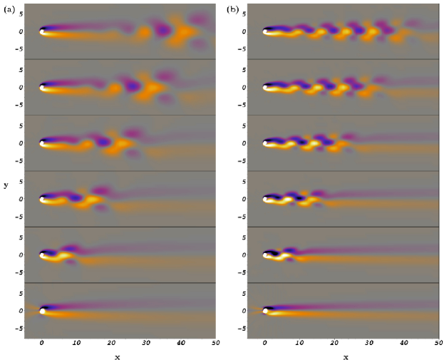
Figure 11: (color online). Same evolution as in Fig. 10, $\mathrm{Re}$=20 (left) and $\mathrm{Re}$=40 (right), but viewed in terms of vorticity. The vorticity of a linear superposition of the base flow and the perturbation is shown at snapshots separated by 10 time units from $t=0$ (bottom) up to $t=50$ (top). The maximum vorticity is 1.5.

To further highlight the spatiotemporal character of the evolving perturbations, and their dependence on $\mathrm{Re}$, we show in Fig. 12 space-time diagrams covering a large range of both space and time. Within each tile, space is horizontal from $x=0$ to $x=125$ and time is vertical from $t=0$ to $t=125$. Hence unit speed, that of the free-stream velocity, corresponds to $45^{\circ}$ in these plots. Each row in this figure corresponds to a particular $\mathrm{Re}$, from $\mathrm{Re}$=20 to $\mathrm{Re}$=50. The left column shows the evolution of energy in the perturbation sampled on the flow centerline, that is, contours of $\mathbf{u^{\prime}}(x,y=0,t)$, where $\mathbf{u^{\prime}}(t=0)=\mathbf{v}_{1}$ is the optimal initial condition. For example, Fig. 12(a) shows the same perturbation as in Fig. 10(a). The contour scale varies from row to row and is set so that the maximum energy corresponds to white and zero energy corresponds to black.

The center and right columns of Fig. 12 are explained as follows. The center column is the evolution of the first sub-dominant optimal mode, that is the evolution of $\mathbf{u^{\prime}}(t)$, where $\mathbf{u^{\prime}}(t=0)=\mathbf{v}_{2}$. The sub-dominant mode and subsequent evolution are very similar to that of the dominant mode. However, careful inspection shows that the sub-dominant mode is spatially phase shifted by a quarter wavelength with respect to the dominant mode. This is seen as a half wavelength shift in Fig. 12 since a pair of vortices (one wavelength) generates two peaks in the centerline energy. The pairing of perturbations has been observed and discussed elsewhere Blackburn et al. (2008a); Cantwell et al. (2010) as a manifestation of streamwise symmetry breaking such that modes come in near pairs with similar, but not identical, dynamics. The importance of this second, phase-shifted mode is that from the pair of modes we can easily construct an approximate energy envelope eliminating the fast oscillations associated with vortex shedding. This is shown in the third column where we plot $E=E_{1}+\alpha E_{2}$, where $E_{1}$ and $E_{2}$ are the energy of the dominant (left column) and sub-dominant (middle column) perturbation fields. We choose $\alpha$ so that the peak energy of the sub-dominant mode matches that of the dominant mode. As one can see this nearly eliminates the fast oscillations throughout the space-time plot of $E$.

The dynamics seen at $\mathrm{Re}$=20, $\mathrm{Re}$=30, and $\mathrm{Re}$=40 are quite similar. There is an increase in energy (both peak energy and spatial extent) followed by a decrease with the long-term dynamics being a weak wave packet propagating and decaying downstream. The effects of varying $\mathrm{Re}$ in the regime are those already noted: there is a decrease in wavelength and an increase near-wake oscillations with increasing $\mathrm{Re}$.

The behavior at $\mathrm{Re}$=45 is, however, qualitatively different from that seen at $\mathrm{Re}$=40 and below, even though $\mathrm{Re}$=45 is still in the subcritical regime. The perturbation at long times does not have a maximum at some downstream location set by how long the perturbation has evolved. Instead the maximum is located at a finite streamwise location. This is due to the fact that at long times the perturbation must evolve to the least stable wake eigenmode and there is a qualitative change in the spatial structure of this eigenmode at $\mathrm{Re}\simeq 42$ (also noted by Giannetti and Luchini who give $\mathrm{Re}\simeq 43$). Below $\mathrm{Re}=42$ the leading eigenmode is exponentially growing downstream and hence appears localized to the downstream computational boundary. Above $\mathrm{Re}=42$ the leading eigenmode has a maximum at finite streamwise position with exponential decay far downstream. The location of the maximum decreases as a function of $\mathrm{Re}$ and is at about $x=34.6$ for $\mathrm{Re}$=45. This phenomenon is well-known and understood in other systems, e.g.  Barkley (1992); Sandstede and Scheel (2000); Wheeler and Barkley (2006). In these systems, the switch from downstream growth to downstream decay of an eigenfunction occurs when the corresponding eigenvalue crosses the essential spectrum. The essential spectrum, in turn, is the continuous eigenvalue spectrum associated with the far-field part of the system. It might be of some interest in the future to investigate these issues for the cylinder wake.

For completeness we also show the evolution at $\mathrm{Re}=50$, slightly into unstable regime. Although somewhat masked by the fact that the perturbation is growing, the spatial structure of the mode at long time is not very different from that at $\mathrm{Re}=45$. The perturbation has a maximum at about $x=19.4$ followed by exponential downstream decay, matching that of the leading eigenmode from the stability analysis at $\mathrm{Re}$=50.

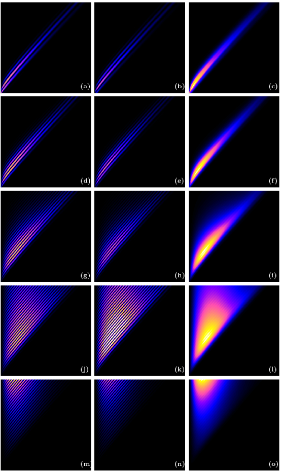
Figure 12: (color online). Plots showing the space-time evolution of energy in the perturbation $\mathbf{u^{\prime}}$. Each tile covers $x$ between 0 and 125 (horizontal) and $t$ between 0 and 125 (vertical), and shows the energy of perturbations sampled on the centerline $y=0$. Each row corresponds to a different Reynolds number, specifically: $\mathrm{Re}=20$ (a,b,c), $\mathrm{Re}=30$ (d,e,f), $\mathrm{Re}=40$ (g,h,i), $\mathrm{Re}=45$ (j,k,l), and $\mathrm{Re}=50$ (m,n,o). For each Reynolds number we show the evolution of the dominant mode (left column), the first sub-dominant mode (center column), and a combination (right column) revealing the envelope of the perturbation as explained in the text. The scale of each row of tiles is normalized by the maximum energy in the right column over the space-time domain, with white corresponding to the highest energy and black to zero energy.

IV.3 3D Energy Growth

We consider here briefly the energy growth of 3D perturbations, mainly to show that 3D effects are unimportant. The spanwise wavenumber $\beta$ of perturbations, Eq. (4), becomes an additional parameter to vary. We shall fix the Reynolds number at $\mathrm{Re}=40$. Optimal growth curves over a range of spanwise wavenumbers, at representative values of $\tau$, are plotted in Fig. 13 and growth contours in the $\beta$-$\tau$ plane are shown in Fig. 14. The thicker line in Fig. 14 denotes the no-growth contour and energy growth occurs only to the left of this contour. Except for small values of $\tau$, the growth of 2D perturbations ($\beta=0$) greatly dominates the growth of 3D perturbations.

For short time horizons, (we estimate $\tau\lesssim 8.0$), the largest possible growth is found at nonzero wavenumbers and the range of active wavenumbers increases considerably as $\tau$ approaches zero. This shift to high-wavenumber modes at short time horizons occurs in other shear flows Schmid and Henningson (1994); Blackburn et al. (2008b); Cantwell et al. (2010), but we are unaware of any explanation for this phenomenon. This does not seem important in any practical sense because the overall response of such modes is very small indeed. We have not investigated other values of $\mathrm{Re}$ in detail, but the unsurprising result is that 2D modes dominate the transient response in the subcritical wake.

Figure 13: Optimal growth as function of spanwise wavenumber $\beta$ at $\mathrm{Re}$=40. $\beta=0$ is dominant for long time horizons, but higher $\beta$ may provide slightly larger growth at short time horizons.

Figure 14: Contour plot of optimal growth at $\mathrm{Re}$=40. The thicker black line denotes the contour of no growth.

V Summary and Discussion

We have studied the subcritical response of the cylinder wake by accurately computing the optimal energy growth throughout the subcritical regime. We have treated at some length the numerical domain requirements for accurate computations within the subcritical region. The results themselves show that energy growth first occurs as low as $\mathrm{Re}\simeq 2.2$, below the onset of separation at $\mathrm{Re}\simeq 6.2$. Over most of the subcritical regime the maximum energy amplification increases approximately exponentially in the square of $\mathrm{Re}$. This super-exponential dependence on $\mathrm{Re}$ is even faster than the exponential dependence commonly observed in other separated flows  Blackburn et al. (2008a, b); Cantwell et al. (2010). However, the maximum growth in the cylinder wake never reaches the extremely large values since the wake becomes linearly unstable at a relatively low $\mathrm{Re}$ where the maximum energy growth is about 6800.

We have considered the structure of the optimal transient dynamics. The evolving perturbations are of the form of transitory Bénard-von Kármán vortex streets. At lower $\mathrm{Re}$ wave packets of only a few wavelengths are formed which propagate downstream. As $\mathrm{Re}$ increases the packets extend in length due to the slow decay of oscillations in the near wake. At $\mathrm{Re}\simeq 42$ the spatial structure of the response at long times switches from exponentially increasing downstream to exponentially decaying downstream so that at about $\mathrm{Re}=42$ the response at long times has a maximum at a finite streamwise location. Finally, at $\mathrm{Re}=\mathrm{Re}_{c}\simeq 46.6$ the wake becomes linearly unstable.

It is of interest to relate our results to the understanding of subcritical dynamics arrived at by local stability analysis, e.g. Monkewitz (1988); Yang and Zebib (1989); Hannemann and Oertel Jr (1989); Huerre and Monkewitz (1990); Delbende and Chomaz (1998); Pier (2002); Chomaz (2005) and references therein. In brief, from sectional stability analysis of wake profiles, the picture of the subcritical region is as follows. Below $\mathrm{Re}\sim 5$ the wake is everywhere stable. Above $\mathrm{Re}\sim 5$ there is a region of convective instability behind the cylinder and at $\mathrm{Re}\sim 25$ a pocket of absolute instability appears within the region of convective instability. The size of the absolute pocket grows with $\mathrm{Re}$ and is thought to be responsible for the actual instability occurring at $\mathrm{Re}_{c}$, although prediction of the transition point has eluded local analysis.

In reality, there are two qualitative changes within the subcritical regime: the onset of transient growth at $\mathrm{Re}$=2.2 and the switch from downstream growth to downstream decay of transient structures at $\mathrm{Re}\simeq 42$, associated with a corresponding change in the structure of eigenmodes. It seems that the first of these, the onset of transient energy growth, could be connected with the first appearance of a local convective instability. A local pocket of convective instability would indeed correspond to transient response in a global setting. Moreover, the $\mathrm{Re}$ values for the two event are reasonably close. This would appear to corroborate the picture first proposed by Cossu and Chomaz Cossu and Chomaz (1997) in the context of the Ginzburg-Landau equation. In this picture, one can understand the transient energy growth as arising from perturbations traveling through a local region of instability, where they are amplified, followed by advection into the stable downstream wake, where they decay. We caution, however, that the cylinder wake is highly non-parallel in the near wake region and it would probably be a mistake to connect the transient response and the parallel-flow analysis in too much detail.

There is nothing in the actual transient response corresponding to the local opening of the absolute pocket at $\mathrm{Re}\sim 25$, but neither is there expected to be Delbende and Chomaz (1998). We have clearly shown an uneventful evolution of the transient response between $\mathrm{Re}=20$ and $\mathrm{Re}=30$, and in fact up to $\mathrm{Re}=40$. We are unaware of any local analysis of the cylinder wake that predicts the shift from growth to decay of modes at $\mathrm{Re}\simeq 42$, and this might be interesting to investigate in the future.

There is another way to view the relationship between our study and concepts of convective and absolute instability. This is also closely related to some past and ongoing experimental studies Le Gal and Croquette (2000); Marais et al. (2010). While convective and absolute instability are strictly defined for streamwise homogeneous flows, which the cylinder wake is not, the change in the linear response at $\mathrm{Re}_{c}$ has the essential character of the transition from convective to absolute instability and it commonly referred to using these terms. One sees this in our Fig. 12 where the subcritical cases, Figs. 12(c), 12(f), 12(i) and 12(l) have the character of convective instability: initial perturbations lead to wave packets that advect downstream such that even though a perturbation grows (for some time) it is simultaneously advected quickly downstream. The supercritical case 12(o) has the character of absolute instability where perturbations grow at fixed streamwise locations. LeGal and Croquette present nice streakline visualizations of the transient wake, qualitatively similar to what is shown in our Fig. 11, and discuss this as evidence of convective instability in the cylinder wake prior to the onset of sustained oscillations. Marias et al. use particle image velocimetry (PIV) to obtain more quantitative measures of the subcritical response generated by rotary motion of the cylinder. In particular they measure front velocities and study how these behave as $\mathrm{Re}_{c}$ is approached. Marias et al. also extract integrated energy from PIV data. Transient amplification is indeed observed, followed by exponential decay. However, due to the fact that experimental perturbations are introduced by cylinder rotation, and not from the optimal initial conditions studied here, quantitative comparisons are not presently possible, but may be pursued in the future.

Finally, we conclude with the issue of numerical accuracy. Our study has highlighted the importance of ensuring the numerical convergence of the computational domain. Transient growth problems in open flows with inflow-outflow boundary conditions are particularly susceptible to deficiencies in the extent of the computational domain. This is true not only in the downstream region, but in the cross-stream and especially the inflow dimensions. It is well known that for external flows enforcing boundary conditions too close to a body can lead to deformation of the underlying basic flow Fornberg (1980); Lecointe and Piquet (1984); Strykowski and Hannemann (1991); Anagnostopoulos et al. (1998). Accurate resolution of perturbation fields for transient growth problems can impose yet more severe requirements. The cylinder wake is a prime example of a flow in which the requisite domain can be far greater for transient growth computations than for other types of calculations.

*

Appendix A

In this appendix we present convergence results for base-flow calculations, stability calculations, and polynomial order.

Base flow convergence is assessed through two indicators: the position, $x_{s}$, of the stagnation point marking the end of the recirculation region and velocity profiles just downstream of the cylinder. Figure 15 summarizes the convergence of the stagnation point with mesh dimension. The stagnation point is not present at $\mathrm{Re}=5$, and consequently this case does not appear. Percentage errors are relative to the calculation using $L_{i}=65$ and $L_{c}=65$, respectively. The stagnation point is seen to be highly converged, as a function of domain dimensions, for $L_{i}=L_{c}=45$.

We may also compare the values of $x_{s}$ with values reported in previous studies Dennis and Chang (1970); Coutanceau and Bouard (1979); Fornberg (1980); Zielinska et al. (1997); Ye et al. (1999); Pier (2002); Giannetti and Luchini (2007). Consistent with other studies, we find for $\mathrm{Re}\geq 6.2$ the stagnation point obeys

$$x_{s}\simeq 0.5+0.067(\mathrm{Re}-6.2),$$

with specific converged values: $x_{s}=1.422$ at $\mathrm{Re}=20$ and $x_{s}=2.762$ at $\mathrm{Re}=40$. These agree very will with recent computational studies by Giannetti and Luchini Giannetti and Luchini (2007) and Ye et al. Ye et al. (1999).

Figure 15: Convergence of the base flow stagnation point with mesh dimensions. Points indicate the computed values. In (a) $L_{c}$ is fixed at 25 and in (b) $L_{i}$ is fixed at 25.

Examination of streamwise velocity profiles is found to provide a more detailed view of base-flow distortion due to the finite-size effects. Figure 16 shows velocity profiles at location $x=3$. Only a limited cross-stream range in $y$ is shown in the vicinity of where the streamwise velocity reaches its maximum, as this is where the effects of domain confinement are most pronounced. Constriction of the cross-stream mesh leads to an especially inaccurate calculation of the base flow, particularly at low $\mathrm{Re}$, while the effect of restricted inflow length is less significant in general [Fig. 16(a) and (c)]. In any case, the base flow is again seen to be highly converged, as a function of domain dimensions, for $L_{i}=L_{c}=45$.

Figure 16: Streamwise velocity profiles of base flows at $\mathrm{Re}$=5, $(a)$ and $(b)$, and at $\mathrm{Re}$=46, $(c)$ and $(d)$, showing variation with $L_{i}$ and $L_{c}$. For variations in $L_{i}$, we fix $L_{c}=25$. For variations in $L_{c}$, we fix $L_{i}=25$.

The dependence of the linear stability calculations on domain size is examined through determination of the critical Reynolds number, $\mathrm{Re}_{c}$, on different domains. For each domain, we compute the base flow and the eigenvalues at $\mathrm{Re}=43,44,45,$ and $46$. From these we extrapolate to find $\mathrm{Re}_{c}$ where the real part of the leading eigenvalue crosses zero. The results are shown in Fig. 17, where as before we report percentage error in the value of $\mathrm{Re}_{c}$ with respect to the value obtained using $L_{i}=65$ and $L_{c}=65$, respectively. Interestingly, one sees very little effect of cross-stream restriction here. In any case, $\mathrm{Re}_{c}$ is well determined for $L_{i}=L_{c}=45$, with an error of less than $0.1\%$.

We may also compare directly the value we obtain for $\mathrm{Re}_{c}$ with that obtained in other studies. To three significant figures, with $L_{i}=L_{c}=45$, we find

$$\mathrm{Re}_{c}=46.6.$$

This value agrees to within half a percent with recent stability calculations by Giannetti and Luchini Giannetti and Luchini (2007) and Marquet et al. Marquet et al. (2008b) who quote values of $\mathrm{Re}_{c}=46.7$ and $\mathrm{Re}_{c}=46.8$, respectively.

Figure 17: Convergence of critical Reynolds number $\mathrm{Re}_{c}$ with mesh size. Points indicate the computed values.

Finally, having set the overall mesh dimensions, we consider the convergence of computations with respect to the polynomial order of the spectral-element expansion. The polynomial order is chosen to ensure there is the necessary refinement to resolve the finest characteristics of the flow at the highest Reynolds number under consideration. Base flow and subsequent transient growth calculations at $\mathrm{Re}=46$ have been carried out for a range of polynomial orders as summarized in Table 2. A polynomial order of $P=6$ is found to be sufficient and is used for all results reported in Sec. IV.

Order	$G(\tau=20)$
3	138.91
4	108.29
5	156.29
6	156.20
7	156.19
8	156.19

Table 2: Convergence of optimal growth results with polynomial order on the mesh $L_{i}=45$, $L_{c}=45$, $L_{o}=125$. The base flow and optimal growth $G(\tau=20)$ at $\mathrm{Re}=46$ are both computed for the polynomial orders indicated.

References

- Zdravkovich (1997) M. M. Zdravkovich, Flow Around Circular Cylinders – Volume 1: Fundamentals (Oxford University Press, 1997).
- Zdravkovich (2003) M. M. Zdravkovich, Flow Around Circular Cylinders – Volume 2: Applications (Oxford University Press, 2003).
- Provansal et al. (1987) M. Provansal, C. Mathis, and L. Boyer, J. Fluid Mech. 182, 1 (1987).
- Jackson (1987) C. Jackson, J. Fluid Mech. 182, 23 (1987).
- Zebib (1987) A. Zebib, Journal of Engineering Mathematics 21, 155 (1987).
- Yang and Zebib (1989) X. Yang and A. Zebib, Phys. Fluids A 1, 689 (1989).
- Dušek et al. (1994) J. Dušek, P. Gal, and P. Fraunié, J. Fluid Mech. 264, 59 (1994).
- Noack and Eckelmann (1994) B. R. Noack and H. Eckelmann, J. Fluid Mech. 270, 297 (1994).
- Pier (2002) B. Pier, J. Fluid Mech. 458, 407 (2002).
- Noack et al. (2003) B. R. Noack, K. Afanasiev, M. Morzyński, G. Tadmor, and F. Thiele, J. Fluid Mech. 497, 335 (2003).
- Chomaz (2005) J.-M. Chomaz, Annu. Rev. Fluid Mech. 37, 357 (2005).
- Barkley (2006) D. Barkley, Europhysics Letters 75, 750 (2006).
- Giannetti and Luchini (2007) F. Giannetti and P. Luchini, J. Fluid Mech. 581, 167 (2007).
- Bénard (1908) H. Bénard, C. R. Acad. Sci. 147, 839 (1908).
- von Kármán (1911) T. von Kármán, Nachr. Ges. Wiss. Goettingen, Math.-Phys. Kl. 12, 509 (1911).
- Schmid and Henningson (2001) P. J. Schmid and D. S. Henningson, Stability and transition in shear flows (Springer Verlag, 2001).
- Trefethen and Embree (2005) L. N. Trefethen and M. Embree, Spectra and Pseudospectra: The Behavior of Nonnormal Matrices and Operators (Princeton University Press, Princeton, 2005).
- Gustavsson (1991) L. Gustavsson, J. Fluid Mech. 224, 241 (1991).
- Butler and Farrell (1992) K. Butler and B. Farrell, Phys. Fluids A 4, 1637 (1992).
- Henningson et al. (1993) D. Henningson, A. Lundbladh, and A. Johansson, J. Fluid Mech. 250, 169 (1993).
- Cossu and Chomaz (1997) C. Cossu and J. M. Chomaz, Phys. Rev. Let. 78, 4387 (1997).
- Åkervik et al. (2007) E. Åkervik, J. Hœpffner, U. Ehrenstein, and D. S. Henningson, J. Fluid Mech. 579, 305 (2007).
- Blackburn et al. (2008a) H. M. Blackburn, D. Barkley, and S. J. Sherwin, J. Fluid Mech. 603, 271 (2008a).
- Marquet et al. (2008a) O. Marquet, D. Sipp, J. M. Chomaz, and L. Jacquin, J. Fluid Mech. 605, 429 (2008a).
- Alizard et al. (2009) F. Alizard, S. Cherubini, and J. Robinet, Phys. Fluids 21, 064108 (2009).
- Blackburn et al. (2008b) H. M. Blackburn, S. J. Sherwin, and D. Barkley, J. Fluid Mech. 607, 267 (2008b).
- Cantwell et al. (2010) C. D. Cantwell, D. Barkley, and H. M. Blackburn, Phys. Fluids 22, 034101 (2010).
- Marquet et al. (2008b) O. Marquet, D. Sipp, and L. Jacquin, J. Fluid Mech. 615, 221 (2008b).
- Abdessemed et al. (2009) N. Abdessemed, A. S. Sharma, S. J. Sherwin, and V. Theofilis, Phys. Fluids 21, 044103 (2009).
- Le Gal and Croquette (2000) P. Le Gal and V. Croquette, Phys. Rev. E 62, 4424 (2000).
- Marais et al. (2010) C. Marais, R. Godoy-Diana, D. Barkley, and J. Wesfreid, Phys. Fluids 00, 0000 (2010).
- Tuckerman and Barkley (2000) L. S. Tuckerman and D. Barkley, in Numerical Methods for Bifurcation Problems and Large-Scale Dynamical Systems, edited by E. Doedel and L. S. Tuckerman (Springer, 2000), pp. 453–566.
- Barkley et al. (2008) D. Barkley, H. M. Blackburn, and S. J. Sherwin, Intnl J. Num. Meth. Fluids 57, 1435 (2008).
- Orszag et al. (1986) S. A. Orszag, M. Israeli, and M. O. Deville, J. Sci. Comp. 1, 75 (1986).
- Karniadakis et al. (1991) G. E. Karniadakis, M. Israeli, and S. A. Orszag, J. Comput. Phys. 97, 414 (1991).
- Blackburn and Sherwin (2004) H. M. Blackburn and S. J. Sherwin, J. Comput. Phys. 197, 759 (2004).
- Fornberg (1980) B. Fornberg, J. Fluid Mech. 98, 819 (1980).
- Lecointe and Piquet (1984) Y. Lecointe and J. Piquet, Computers & Fluids 12, 255 (1984).
- Strykowski and Hannemann (1991) P. Strykowski and K. Hannemann, Acta Mechanica 90, 1 (1991).
- Anagnostopoulos et al. (1998) P. Anagnostopoulos, G. Iliadis, and S. Richardson, International Journal for Numerical Methods in Fluids 22, 1061 (1998).
- Joseph (1976) D. D. Joseph, Stability of Fluid Motions I (Springer-Verlag, Berlin, 1976).
- Barkley (1992) D. Barkley, Phys. Rev. Let. 68, 2090 (1992).
- Sandstede and Scheel (2000) B. Sandstede and A. Scheel, Phys. Rev. E 62, 7708 (2000).
- Wheeler and Barkley (2006) P. Wheeler and D. Barkley, SIAM J. Appl. Dyn. Syst. 5, 157 (2006).
- Schmid and Henningson (1994) P. J. Schmid and D. S. Henningson, J. Fluid Mech. 277, 197 (1994).
- Monkewitz (1988) P. A. Monkewitz, Phys. Fluids 31, 999 (1988).
- Hannemann and Oertel Jr (1989) K. Hannemann and H. Oertel Jr, J. Fluid Mech. 199, 55 (1989).
- Huerre and Monkewitz (1990) P. Huerre and P. A. Monkewitz, Annu. Rev. Fluid Mech. 22, 473 (1990).
- Delbende and Chomaz (1998) I. Delbende and J. Chomaz, Phys. Fluids 10, 2724 (1998).
- Dennis and Chang (1970) S. C. R. Dennis and G. Z. Chang, J. Fluid Mech. 42, 471 (1970).
- Coutanceau and Bouard (1979) M. Coutanceau and R. Bouard, J. Fluid Mech. 79, 231 (1979).
- Zielinska et al. (1997) B. J. A. Zielinska, S. Goujon-Durand, J. Dusek, and J. E. Wesfreid, Phys. Rev. Let. 79, 3893 (1997).
- Ye et al. (1999) T. Ye, R. Mittal, H. S. Udaykumar, and W. Shyy, J. Comput. Phys. 156, 209 (1999).