Low-lying even parity meson resonances and spin-flavor symmetry revisited

Abstract

We review and extend the model derived in Phys. Rev. D 83 016007 (2011) to address the dynamics of the low-lying even parity meson resonances. This model is based on a coupled channels spin-flavor extension of the chiral Weinberg-Tomozawa Lagrangian. This interaction is then used to study the $S$-wave meson-meson scattering involving members not only of the $\pi$-octet, but also of the $\rho$-nonet. In this work, we study in detail the structure of the SU(6) symmetry breaking contact terms that respect (or softly break) chiral symmetry. We derive the most general local (without involving derivatives) terms consistent with the chiral symmetry breaking pattern of QCD. After introducing sensible simplifications to reduce the large number of possible operators, we carry out a phenomenological discussion of the effects of these terms. We show how the inclusion of these pieces leads to an improvement of the description of $J^{P}=2^{+}$ sector, without spoiling the main features of the predictions obtained in the original model in the $J^{P}=0^{+}$ and $J^{P}=1^{+}$ sectors. In particular, we find a significantly better description of the $I^{G}(J^{PC})=0^{+}(2^{++}),1^{-}(2^{++})$ and the $I(J^{P})=\frac{1}{2}(2^{+})$ sectors, which correspond to the $f_{2}(1270)$, $a_{2}(1320)$ and $K^{*}_{2}(1430)$ quantum numbers, respectively.

I Introduction

The study of the lowest–lying hadron resonances dynamics has received a lot of attention in the last decades, in particular since it was realized that some of them cannot be easily accommodated as radial or angular excitations of the Constituent Quark Model (CQM) ground states. Some examples are the low-lying scalar $f_{0}(500)$, $f_{0}(980)$, $a_{0}(980)$ and $K^{*}_{0}(800)$, or axial vector $a_{1}(1260)$, $b_{1}(1235)$, $h_{1}(1170)$, $f_{1}(1285)$, $K_{1}(1270)$ mesons. The field has experimented a considerable boost in the last five years, because several clear candidates for exotic states can be found among the recently discovered hidden bottom and charm $XYZ$ resonances reported by the Belle, BABAR, $D0$ and CDF collaborations. There has been a steady activity in the context of CQM’s aiming to supplement these models with exotic components due to existence of tetraquark degrees of freedom inside of the hadrons (see for instance the discussion in Ref. Vijande:2007ix ). Such components might lead to extended CQM schemes where the known exotic resonances could be generated and their main features be described. Here, however, we will pay attention to a different approach, in which the hadron resonances appear as bound or resonant states of an interacting pair of ground state hadrons (mesons of the $\pi$ octet and the $\rho$ nonet and baryons of the $N$ octet and $\Delta(1232)$ decuplet, when the study is limited to the three lightest quark flavors). In this molecular picture, hadron resonances show up as poles in the First or Second Riemann Sheets (FRS/SRS) of certain hadron–hadron amplitudes. The positions of the poles determine masses and widths of the resonances, while the residues for the different channels define the corresponding coupling or branching fractions. The interaction among the ground state hadrons is thus the first ingredient to build this molecular scheme. These are usually obtained from Effective Field Theories (EFT’s) that incorporate constrains deduced from some relevant exact or approximate symmetries of Quantum Chromodynamics (QCD). In this context, it is clear that Chiral Perturbation Theory (ChPT) Weinberg:1978kz ; Gasser:1983yg ; Gasser:1984gg and Heavy Quark Spin Symmetry (HQSS) IW89 ; Ne94 ; MW00 should play relevant roles, when designing interactions involving Goldstone bosons or charm/bottom hadrons, respectively. In this work, we will focus in the light SU(3) flavor sector and we will leave the extension of this discussion to heavy molecules for future research.

ChPT is a systematic implementation of chiral symmetry and of its pattern of spontaneous and explicit breaking, and it provides a model independent scheme where a large number of low-energy non-perturbative strong-interaction phenomena can be understood. It has been successfully applied to study different processes involving light ($u$ and $d$) or strange ($s$) quarks. Because ChPT provides the scattering amplitudes as a perturbative series, it cannot describe non-analytical features as poles. Thus, ChPT cannot directly describe the nature of hadron resonances. In recent years, it has been shown that by unitarizing the ChPT amplitudes in coupled channels, the region of application of ChPT can be greatly extended. This approach, commonly referred as Unitary Chiral Perturbation Theory (UChPT), has received much attention and provided many interesting results, in particular in the meson-meson sector where we will concentrate our attention in this work, Truong:1988zp ; Dobado:1989qm ; Dobado:1992ha ; Dobado:1996ps ; Hannah:1997ux ; Oller:1997ng ; Oller:1997ti ; Nieves:1998hp ; Kaiser:1998fi ; Oller:1998hw ; Oller:1998zr ; Nieves:1999bx ; Nieves:2001de ; GomezNicola:2001as ; Lutz:2003fm ; Roca:2005nm ; Geng:2006yb ; GomezNicola:2007qj ; Molina:2008jw ; Geng:2008gx ; Albaladejo:2008qa ; GarciaRecio:2010ki . It turns out that many meson-meson resonances and bound states appear naturally within UChPT. These states are then interpreted as having “dynamical nature.” In other words, they are not genuine $q\bar{q}$ states, but are mainly built out of their meson-meson components. To distinguish among these two pictures, it has been suggested to follow the dependence on a variable number of colors $N_{C}(>3)$ of the resonance properties by assuming that hadronic properties scale similarly as if $N_{C}$ was large. Some interesting results are being obtained from this perspective Pelaez:2003dy ; Pelaez:2006nj ; Geng:2008ag ; Nieves:2009ez ; Nieves:2009kh ; Nieves:2011gb ; Guo:2011pa , and at present there exists some controversy on the nature of the $f_{0}(500)$ resonance Pelaez:2006nj ; Nieves:2011gb ; Guo:2011pa for which accurate models are available.

The present work is an update of Ref. GarciaRecio:2010ki , where was derived a spin-flavor extension of chiral symmetry to study the $S$-wave meson-meson interaction involving members not only of the $\pi$-octet, but also of the $\rho$-nonet. The similar approach for baryon-meson dynamics was initiated in GarciaRecio:2005hy ; GarciaRecio:2006wb . Elastic unitarity in coupled channels is restored in GarciaRecio:2010ki by solving a renormalized coupled-channel Bethe–Salpeter Equation (BSE) with an interaction kernel deduced from spin-flavor extensions of the ChPT amplitudes. In the scheme of Ref. GarciaRecio:2010ki , the spin-flavor symmetry was explicitly broken to account for physical masses and decay constants of the involved mesons, and also when the amplitudes were renormalized. Nevertheless, the underlying SU(6) symmetry was still present and served to organize the set of even parity meson resonances found in that work. Indeed, it was shown that most of the low-lying even parity PDG (Particle Data Group Collaboration Beringer:1900zz ) meson resonances, specially in the $J^{P}=0^{+}$ and $1^{+}$ sectors, could be classified according to multiplets of the SU(6) spin-flavor symmetry group. However, some resonances, like the isoscalar $f_{0}(1500)$ or $f_{1}(1420)$ states, could not be accommodated within this scheme and it was claimed that these states could be clear candidates to be glueballs or hybrids GarciaRecio:2010ki .

Chiral symmetry (CS), and its breaking pattern, is encoded in the approach of Ref. GarciaRecio:2010ki at leading order (LO) by means of the Weinberg-Tomozawa (WT) soft pion theorem Weinberg:1966kf ; Tomozawa:1966jm . This CS input strongly constraints the pseudoscalar–pseudoscalar ($PP$) and pseudoscalar–vector ($PV$) channels, since the mesons of the pion octet were identified with the set of Nambu-Goldstone bosons that appear for three flavors (due to the spontaneous breaking of CS). Thus, the main features (masses, widths, branching fractions and couplings) of the lowest nonet of $S$-wave scalar resonances ($f_{0}(500)$, $f_{0}(980)$, $a_{0}(980)$ and $K^{*}_{0}(800)$) found in Ref. GarciaRecio:2010ki do not significantly differ from those obtained in previous SU(3) UChPT approaches Oller:1997ti ; Oller:1998hw ; GomezNicola:2001as . This is because these resonances are generated from the interaction of Nambu-Goldstone bosons, and the influence of the vector–vector ($VV$) components in these states is small.

The $PV$ and $VV$ sectors have been also systematically studied in Refs. Roca:2005nm and Molina:2008jw ; Geng:2008gx , respectively. These works adopt the formalism of the hidden gauge interaction for vector mesons Bando:1984ej ; Bando:1987br . In the $PV\to PV$ sector, as mentioned above, CS constrains the interactions, and the interactions derived in Ref. GarciaRecio:2010ki and those used in Ref. Roca:2005nm totally agree at LO in the chiral expansion, despite their different apparent structure and origin. As a consequence, the results of Ref. GarciaRecio:2010ki are in general in good agreement with those previously obtained in Ref. Roca:2005nm , which among others include the prediction of a two pole structure for the $K_{1}(1270)$ resonance Geng:2006yb . However, the simultaneous consideration of $PV$ and $VV$ channels made the approach of Ref. GarciaRecio:2010ki different from that followed in Ref. Roca:2005nm in few cases. One of the most remarkable cases was that of the $h_{1}(1595)$ resonance, which was dynamically generated for the first time in the work of Ref. GarciaRecio:2010ki . The interference $PV\to VV$ amplitudes turned out to play a crucial role in producing this state in GarciaRecio:2010ki , and that is presumably the reason why the $h_{1}(1595)$ resonance was generated neither in the $PV\to PV$ study of Roca:2005nm , nor in the $VV\to VV$ scheme of Ref. Geng:2008gx . Possibly, the situation is similar for the $K_{1}(1650)$ state. These two resonances helped to envisage a clearer SU(6) pattern in  GarciaRecio:2010ki , which is also followed to some extent in nature, and that is missed in the separate works of Refs. Roca:2005nm and  Geng:2008gx .

In general terms, the model of Ref. GarciaRecio:2010ki provides a fairly good description of the $J^{P}=0^{+}$ and $J^{P}=1^{+}$ sectors. However, from a phenomenological point of view, the model of Ref. GarciaRecio:2010ki led to a much poorer description of the $J^{P}=2^{+}$ sector, which for $S$-wave is constructed out of $VV$ interactions. Indeed, the well established $f_{2}(1270)$ and $K^{*}_{2}(1430)$ resonances are difficult to accommodate in the scheme, which needs to be somehow pushed to its limits of validity. The hidden gauge interaction for vector mesons model used in Geng:2008gx seems to be more successful in describing the properties of the $f_{2}(1270)$ and $K^{*}_{2}(1430)$ resonances. This latter model and that of Ref. GarciaRecio:2010ki are related for $PV\to PV$ scattering, thanks to CS, but they are completely unrelated in the $VV$ sector.

The SU(6) spin-flavor symmetry is severely broken in nature. Certainly it is mandatory to take into account mass breaking effects by using different pseudoscalar and vector mesons masses. However, this cannot be done by just using these masses in the kinematics of the amplitudes derived in a straight SU(6) extension of the WT Lagrangian, since this would lead to flagrant violations of the soft pion theorems in the $PV\to PV$ sector due to the large vector meson masses. Instead in  GarciaRecio:2010ki , a proper mass term was added to the extended WT Lagrangian that produced different pseudoscalar and vector meson masses, while preserving, or softly breaking, chiral symmetry. Such term, besides providing masses to the vector mesons, gives rise to further contact interaction terms (local). However, some other local interaction SU(6) symmetry breaking terms respecting (softly breaking) CS can be designed, as we show in this work. The nature of the contact terms can only be fully unraveled by requiring consistency with the QCD asymptotic behavior at high energies Ecker:1989yg , which is far from being trivial. As an alternative, we will present here a phenomenological analysis of the effects on the resonance spectrum due to the inclusion of new VV interactions consistent with CS. Thus, in first place, we will find in this work the most general four meson-field local (involving no derivatives) terms consistent with the chiral symmetry breaking pattern of QCD, and constructed by using a single trace, in the spirit of the large $N_{C}$ expansion. Next, we will show that the inclusion of these pieces leads to a considerable improvement of the description of $J^{P}=2^{+}$ sector, without spoiling the main features of the predictions obtained in Ref. GarciaRecio:2010ki for the $J^{P}=0^{+}$ and $J^{P}=1^{+}$ sectors.

The paper is organized as follows. First, we briefly review in Sect. II the model derived in Ref. GarciaRecio:2010ki , including a brief discussion (Subsect. II.2) on the BSE in coupled channels, and the renormalization scheme used to obtain finite amplitudes. Next in Sect. III, we study the interplay between the SU(6) symmetry breaking local terms and CS, and design two new interaction terms. Their phenomenological implications are studied in Sect. IV. There, we present results in terms of the unitarized amplitudes and search for poles on the complex plane. We discuss the results sector by sector trying to identify the obtained resonances or bound states with their experimental counterparts Beringer:1900zz , and compare our results with earlier studies, in particular that of Ref. GarciaRecio:2010ki . A brief summary and some conclusions follow in Sect. V. In Appendix A, we show that there are just three chiral invariant four meson contact interactions, if only a single trace is allowed to construct them. In Appendix B the various potential matrices derived in this work are compiled for the different hypercharge, isospin and spin sectors.

II SU(6) extension of the SU(3)-flavor Weinberg-Tomozawa Lagrangian

In this section, we briefly review the model derived in Ref. GarciaRecio:2010ki to describe the $S$-wave interaction of four mesons of the $\pi$-octet and/or $\rho$-nonet.

II.1 The interaction

In Ref. GarciaRecio:2010ki , the BSE was solved by using as a kernel the amplitude ${\mathcal{H}}$ given by Eq. (40) of Ref. GarciaRecio:2010ki . This amplitude consists of three different contributions. Two of them (${\mathcal{D}}_{\mathrm{kin}}$ and ${\mathcal{D}}_{a}$) come from the straight extension to SU(6) of the kinetic part of the LO WT SU(3)–flavor interaction, while the third one, ${\mathcal{D}}_{m}$, is originated by the mechanism implemented in GarciaRecio:2010ki to give different masses to pseudoscalar and vector mesons. To give mass to the vector mesons certainly requires breaking SU(6) in the Lagrangian, not only through mass terms but also by interaction terms, due to chiral symmetry.

The lowest-order chiral Lagrangian describing the interaction of pseudoscalar Nambu-Goldstone bosons is Gasser:1984gg

$$\mathcal{L}=\frac{f^{2}}{4}{\mathrm{tr}}\left(\partial_{\mu}U^{\dagger}\partial^{\mu}U+\mathcal{M}(U+U^{\dagger}-2)\right),$$ (1)

where $f\sim 90\,{\mathrm{MeV}}$ is the chiral-limit pion decay constant, $U=e^{{\rm i}\sqrt{2}\Phi/f}$ is a unitary $3\times 3$ matrix that transforms under the linear realization of SU(3)${}_{\rm L}\otimes$SU(3)_R, with

$$\Phi=\left(\begin{array}[]{ccc}\frac{1}{\sqrt{6}}\eta+\frac{1}{\sqrt{2}}\pi^{0}&\pi^{+}&K^{+}\\ \pi^{-}&\frac{1}{\sqrt{6}}\eta-\frac{1}{\sqrt{2}}\pi^{0}&K^{0}\\ K^{-}&\bar{K}^{0}&-\sqrt{\frac{2}{3}}\eta\end{array}\right),$$ (2)

and the mass matrix $\mathcal{M}=\mathrm{diag}(m_{\pi}^{2},m_{\pi}^{2},2m_{K}^{2}-m_{\pi}^{2})$ is determined by the pion and kaon meson masses.

The straight SU(6) extension of Eq. (1) from SU(3) to SU(6) is GarciaRecio:2010ki

$$\mathcal{L}_{\mathrm{SU(6)}}=\frac{f^{2}_{6}}{4}{\mathrm{tr}}\!\left(\partial_{\mu}U^{\dagger}_{6}\partial^{\mu}U_{6}+\mathcal{M}_{6}(U_{6}+U_{6}^{\dagger}-2)\right),\qquad U_{6}=e^{{\rm i}\sqrt{2}\Phi_{6}/f_{6}}.$$ (3)

where $U_{6}$ is now a unitary $6\times 6$ matrix that transforms under the linear realization of SU(6)${}_{\rm L}\otimes$SU(6)_R. The Hermitian matrix $\Phi_{6}$ is the meson field in the 35 irreducible representation of SU(6), and $f_{6}=f/\sqrt{2}$ GarciaRecio:2006wb . SU(6) spin-flavor symmetry allows to assign the vector mesons of the $\rho$ nonet and the pseudoscalar mesons of the $\pi$ octet in the same (35) SU(6) multiplet. A suitable choice for the $\Phi_{6}$ field is

$$\Phi_{6}=\underbrace{P_{a}\frac{\lambda_{a}}{\sqrt{2}}\otimes\frac{I_{2\times 2}}{\sqrt{2}}}_{{\displaystyle{\Phi_{P}}}}+\underbrace{R_{ak}\frac{\lambda_{a}}{\sqrt{2}}\otimes\frac{\sigma_{k}}{\sqrt{2}}+W_{k}\frac{\lambda_{0}}{\sqrt{2}}\otimes\frac{\sigma_{k}}{\sqrt{2}}}_{\displaystyle{\Phi_{V}}},\quad a=1,\ldots,8,\quad k=1,2,3$$ (4)

with $\lambda_{a}$ the Gell-Mann and ${\bm{\sigma}}$ the Pauli spin matrices, respectively, and $\lambda_{0}=\sqrt{2/3}\,I_{3\times 3}$ ($I_{n\times n}$ denotes the identity matrix in the $n$ dimensional space). $P_{a}$ are the $\pi,K,\eta$ fields, while $R_{ak}$ and $W_{k}$ stand for the $\rho$-vector nonet fields, considering explicitly the spin degrees of freedom.

The first term in $\mathcal{L}_{\mathrm{SU(6)}}$ preserves both chiral and spin-flavor symmetries. The second term breaks explicitly chiral symmetry, and taking for instance $\mathcal{M}_{6}=m_{6}I_{6\times 6}$, provides a common mass, $m_{6}$, for all mesons belonging to the SU(6) 35 irreducible representation. However, the SU(6) spin-flavor symmetry is severely broken in nature and it is indeed necessary to take into account mass breaking effects by using different pseudoscalar and vector mesons masses.

To this end in Ref. GarciaRecio:2010ki , the following mass term, which replaces that in Eq. (3), was considered

$$\mathcal{L}_{\mathrm{SU(6)}}^{(m)} = \frac{f^{2}_{6}}{4}{\mathrm{tr}}\!\left({\mathcal{M}}(U_{6}+U_{6}^{\dagger}-2)\right)+\frac{f^{2}_{6}}{32}{\mathrm{tr}}\!\left({\mathcal{M}}^{\prime}({\bm{\sigma}}\,U_{6}\,{\bm{\sigma}}\,U^{\dagger}_{6}+{\bm{\sigma}}\,U_{6}^{\dagger}\,{\bm{\sigma}}\,U_{6}-6)\right).$$ (5)

Here the matrix ${\mathcal{M}}$ acts only in flavor space and it is to be understood as ${\mathcal{M}}\otimes I_{2\times 2}$, and similarly for ${\mathcal{M}}^{\prime}$, so that SU(2)_spin invariance is preserved by these mass matrices. Besides, these matrices should be diagonal in the isospin basis of Eq. (2) so that charge is conserved. Also, ${\bm{\sigma}}$ stands for $I_{3\times 3}\otimes{\bm{\sigma}}$.

The first term in $\mathcal{L}_{\mathrm{SU(6)}}^{(m)}$ is fairly standard. It preserves spin-flavor symmetry when ${\mathcal{M}}$ is proportional to the identity matrix and introduces a soft breaking of chiral symmetry when ${\mathcal{M}}$ is small. This term gives the same mass to pseudoscalar and vector mesons multiplets. Note that terms of this type are sufficient to give different mass to pseudoscalars (e.g. $\pi$ and $K$) when SU($N_{F})$ is embedded into SU($N_{F}^{\prime}$) (a larger number of flavors). They are not sufficient however to provide different $P$ and $V$ masses when SU($N_{F}$) is embedded into SU($2N_{F}$) (spin-flavor).

The second term in $\mathcal{L}_{\mathrm{SU(6)}}^{(m)}$ only gives mass to the vector mesons: indeed, if one would retain in $U_{6}$ only the pseudoscalar mesons, $U_{6}$ would cancel with $U_{6}^{\dagger}$ (since these matrices would commute with ${\bm{\sigma}}$) resulting in a cancellation of the whole term. This implies that this term does not contain contributions of the form $PP$ (pseudoscalar mass terms) nor $PPPP$ (purely pseudoscalar interaction). In addition, when ${\mathcal{M}}^{\prime}$ is proportional to the identity matrix (i.e., exact flavor symmetry) chiral symmetry is also exactly maintained, because the chiral rotations of $U_{6}$ commute with ${\bm{\sigma}}$. This guarantees that this term will produce the correct $PV\to PV$ contributions to ensure the fulfillment of soft pion WT theorem Weinberg:1966kf ; Tomozawa:1966jm even when the vector mesons masses are not themselves small.

At order $\Phi_{6}^{2}$, the Lagrangian of Eq. (5) provides proper mass terms for $P$ and $V$ mesons, while at order $\Phi_{6}^{4}$ it gives rise to four meson interaction terms. In the exploratory study of Ref. GarciaRecio:2010ki , the chiral breaking mass term ($\mathcal{M}$) was neglected, and a common mass, $m_{V}$, for all vector mesons ($\mathcal{M}^{\prime}=m_{V}^{2}I_{3\times 3}\,I_{2\times 2}$) was used. With these simplifications, the interaction piece deduced from $\mathcal{L}_{\mathrm{SU(6)}}^{(m)}$ reads GarciaRecio:2010ki

$$\mathcal{L}_{\mathrm{SU(6)}}^{(m;\,{\rm int})} = \frac{m_{V}^{2}}{8f^{2}}{\mathrm{tr}}\!\left(\Phi_{6}^{4}+{\bm{\sigma}}\,\Phi_{6}^{2}\,{\bm{\sigma}}\Phi_{6}^{2}-\frac{4}{3}{\bm{\sigma}}\,\Phi_{6}\,{\bm{\sigma}}\,\Phi_{6}^{3}\right).$$ (6)

This term gives rise to the local ${\mathcal{D}}_{m}$ contribution to the four meson amplitude ${\mathcal{H}}$ in Eq. (40) of Ref. GarciaRecio:2010ki . The other two contributions, ${\mathcal{D}}_{\mathrm{kin}}$ and ${\mathcal{D}}_{a}$, to ${\mathcal{H}}$ come from the first term (kinetic) of $\mathcal{L}_{{\mathrm{SU}}(6)}$ in Eq. (3). In addition, in Ref. GarciaRecio:2010ki were also considered spin-flavor symmetry-breaking effects due to the difference between pseudoscalar- and vector-meson decay constants, and an ideal mixing between the $\omega$ and $\phi$ mesons (see Subsect. IID of Ref. GarciaRecio:2010ki for some more details, and Table II for the values of the meson and decay constants used in the numerical calculations).

II.2 Scattering Matrix and coupled-channel unitarity

The four meson amplitude ${\mathcal{H}}$ of Eq. (40) of Ref. GarciaRecio:2010ki is used as kernel of the BSE, which is solved and renormalized for each $YIJ$ (hypercharge, isospin and spin) sector in the so called on-shell scheme Nieves:1999bx , $T^{YIJ}$ is given by

$$T^{YIJ}(s)=\frac{1}{1-V^{YIJ}(s)\,G^{YIJ}(s)}V^{YIJ}(s).$$ (7)

where $V^{YIJ}(s)$ (a matrix in the coupled-channel space) stands for the projection of the scattering amplitude, ${\mathcal{H}}$, in the $YIJ$ sector. The corresponding quantity in the present work is defined below by Eqs. (19), (20) and (21). $\sqrt{s}$ is the center or mass energy of the initial or final meson pair. $G^{YIJ}(s)$ is the loop function and it is diagonal in the coupled-channel space. Suppressing the indices, it is written for each channel as

$$G(s)=\bar{G}(s)+G((m_{1}+m_{2})^{2}).$$ (8)

The finite function $\bar{G}(s)$ can be found in Eq. (A9) of Ref. Nieves:2001wt , and it displays the unitarity right-hand cut of the amplitude. On the other hand, the constant $G((m_{1}+m_{2})^{2})$ contains the logarithmic divergence. After renormalizing using the dimensional regularization scheme, one finds

$$G(s=(m_{1}+m_{2})^{2})=\frac{1}{16\pi^{2}}\left(a(\mu)+\frac{2}{m_{1}+m_{2}}\left\{m_{1}\ln\frac{m_{1}}{\mu}+m_{2}\ln\frac{m_{2}}{\mu}\right\}\right)$$ (9)

where $\mu$ is the scale of the dimensional regularization. Changes in the scale are reabsorbed in the subtraction constant $a(\mu)$, so that the results remain scale independent. Any reasonable value for $\mu$ can be used. In Ref. GarciaRecio:2010ki $\mu=1\,{\mathrm{GeV}}$ was adopted and we take the same choice in the present work.

Poles, $s_{R}$, in the SRS of the corresponding BSE scattering amplitudes ($T^{YIJ}(s)$) determine the masses and widths of the dynamically generated resonances in each $YIJ$ sector (namely $s_{R}=M^{2}_{R}-{\rm i}\ M_{R}\Gamma_{R}$). In some cases, there appear real poles in the FRS of the amplitudes which correspond to bound states. Finally, the coupling constants of each resonance to the various meson-meson states ($i,j$ indices) are obtained from the residues at the pole, by matching the BSE amplitudes to the expression

$$T^{YIJ}_{ij}(s)=\frac{g_{i}g_{j}}{s-s_{R}}\,,$$ (10)

for energy values $\sqrt{s}$ close to the pole. The couplings, $g_{i}$, are complex in general.

III SU(6) symmetry breaking terms and chiral invariance

Regarding the spin symmetry breaking term of $\mathcal{L}_{\mathrm{SU(6)}}^{(m)}$ (the term with ${\mathcal{M}}^{\prime}$ in Eq. (5)), it should be noted that there is a large ambiguity in choosing it. Being a contact term, it cannot contain $PPPP$ contributions, due to chiral symmetry, and for the same reason the terms $PPVV$ are also fixed, as already noted. However, $VVVV$ terms are not so constrained. One can easily propose alternative forms for $\mathcal{L}_{\mathrm{SU(6)}}^{(m)}$ which would still be acceptable from general requirements but would yield different $VVVV$ interactions. The choice in Eq. (5) is just the simplest or minimal one.

Let us consider the contact or ultra-local terms, i.e., involving no derivatives, that can be written down with the desired properties. These properties include hermiticity, $C$, $P$ and $T$, invariance under rotations and chiral symmetry. Of course, spin-flavor cannot be maintained, as we want to give different masses to pseudoscalar and vector mesons.

In the absence of derivatives, the parity transformation is equivalent to $U_{6}\to U_{6}^{\dagger}$, likewise, $C$ implies $U_{6}\to U_{6}^{T}$ (transposed), and time-reversal is $U_{6}\to U_{6}$ but acting antilinearly. As it turns out, $C$ and $T$ invariances are automatically implied by the other symmetries if the coupling constants are real (o purely imaginary if $\epsilon_{ijk}$ is involved).

Rotational invariance is ensured if the only tensors involved are Pauli matrices, as well as $\delta_{ij}$ and $\epsilon_{ijk}$.

Under chiral transformations $U_{6}\to\Omega_{L}^{\dagger}U_{6}\Omega_{R}$, where $\Omega_{L,R}$ are matrices of ${\mathrm{SU}}(N_{F})$, (so actually, they denote $2N_{F}\times 2N_{F}$ matrices of the form $\Omega_{L,R}\times I_{2\times 2}$). Vector invariance ($\Omega_{L}=\Omega_{R}$), the diagonal part of the chiral group, is automatic if the operators are constructed as traced products of $U_{6}$, $U_{6}^{\dagger}$ and ${\bm{\sigma}}$ that commutes with the flavor matrices $\Omega_{L,R}$. Note that the matrix ${\mathcal{M}}^{\prime}$ in Eq. (5) must be a multiple of the identity if vector invariance is exactly enforced, as we do in this discussion. Finally, full chiral invariance requires that $U_{6}$ and $U_{6}^{\dagger}$ blocks should occupy alternate positions in the trace (cyclically), with Pauli matrices inserted in between.

A closer look shows that there should be at least one ${\bm{\sigma}}$ between consecutive $U_{6}$ and $U_{6}^{\dagger}$ (cyclically), and also no more than one ${\bm{\sigma}}$ is required due to the relation $\sigma_{i}\sigma_{j}=\delta_{ij}+{\mathrm{i}}\epsilon_{ijk}\sigma_{k}$. Therefore the total number of ${\bm{\sigma}}$ operators is even and so the number of $\epsilon_{ijk}$ is also even. This implies that no Levi-Civita tensor $\epsilon_{ijk}$ is needed, due to the identity

$$\epsilon_{ijk}\epsilon_{abc}=\delta_{ia}\delta_{jb}\delta_{kc}+\delta_{ib}\delta_{jc}\delta_{ka}+\delta_{ic}\delta_{ja}\delta_{kb}-\delta_{ia}\delta_{jc}\delta_{kb}-\delta_{ic}\delta_{jb}\delta_{ka}-\delta_{ib}\delta_{ja}\delta_{kc}.$$ (11)

This leads us to the conclusion that the most general contact interaction with the required symmetries are traced products of blocks

$$\mathcal{U}_{ij}=\sigma_{i}U_{6}\sigma_{j}U_{6}^{\dagger},$$ (12)

that is, products of blocks ${\mathrm{tr}}(\mathcal{U}_{ij}\mathcal{U}_{kl}\cdots)$, with the indices contracted in any order.

In principle, there is an infinite number of such interactions (although relations among them do appear if a concrete number of flavors, say $N_{F}=3$, is assumed). Nevertheless, the interaction is not needed to all orders in the meson field $\Phi_{6}$, rather only quadratic and quartic terms need to be retained. Clearly, there is just a finite number of such $O(\Phi_{6}^{2})+O(\Phi_{6}^{4})$ chiral invariant terms, for the simple reason that only a finite number of quadratic plus quartic structures can be written down. Without assuming chiral symmetry there are $21$ such generic structures (and only $18$ if $N_{F}=3$ is specifically assumed). Chiral symmetry imposes relations and reduces the number from 21 to 10 (9 if $N_{F}=3$ is assumed). This is a rather large number of parameters. In order to reduce the problem to a more manageable size, we will consider here only terms with just a single trace (rather than products of them). We only mention that such restriction can be justified from large $N_{C}$ arguments 'tHooft:1974hx ; Witten:1979kh . The restriction to a single trace puts conditions on the possible mass terms for the vector mesons, specifically ${\mathrm{tr}}(\Phi_{6}^{2})$ and ${\mathrm{tr}}((\sigma_{i}\Phi_{6})^{2})$ are allowed but $({\mathrm{tr}}(\sigma_{i}\Phi_{6}))^{2}$ is discarded. This implies that the $\rho$ and $\omega$ mesons cannot be given different masses. Such degeneracy is very well satisfied experimentally and this gives some basis to our simplifying assumption.

If only terms with a single trace are retained, the number of possible quadratic plus quartic operators is 8, and just 3 combinations of them are chirally invariant. We show this in detail in Appendix A.

The 3 chiral invariant combinations can be obtained by expanding three independent operators of the type ${\mathrm{tr}}(\mathcal{U}_{ij}\mathcal{U}_{kl}\cdots)$ to order $\Phi_{4}^{4}$. Up to two $\mathcal{U}_{ij}$ blocks and a single trace, only three different operators can be written down, and they are sufficient for our purposes:

$${\mathcal{O}}_{1} = {\mathrm{tr}}\!\left(\mathcal{U}_{ii}-3\right),$$

$${\mathcal{O}}_{2} = {\mathrm{tr}}\!\left(\mathcal{U}_{ii}\mathcal{U}_{jj}-9\right)+\mbox{h.c.},$$ (13)

$${\mathcal{O}}_{3} = {\mathrm{tr}}\!\left(\mathcal{U}_{ij}\mathcal{U}_{ij}+3\right).$$

Expanding in the fields, we find

$${\mathcal{O}}_{1} = \frac{3}{f^{2}}{\mathrm{tr}}\!\left(-4\Phi_{6}^{2}+\frac{4}{3}\sigma_{i}\Phi_{6}\sigma_{i}\Phi_{6}\right)+\frac{4}{f^{4}}{\mathrm{tr}}\!\left(\Phi_{6}^{4}+\sigma_{i}\,\Phi_{6}^{2}\,\sigma_{i}\Phi_{6}^{2}-\frac{4}{3}\sigma_{i}\,\Phi_{6}\,\sigma_{i}\,\Phi_{6}^{3}\right)+{\mathcal{O}}(\Phi_{6}^{6})$$ (14)

$$\frac{{\mathcal{O}}_{2}-20{\mathcal{O}}_{1}}{12} = \frac{16}{f^{4}}{\mathrm{tr}}\!\left(\Phi_{6}^{4}+\frac{5}{6}\sigma_{i}\,\Phi_{6}^{2}\,\sigma_{i}\Phi_{6}^{2}-\frac{4}{3}\sigma_{i}\,\Phi_{6}\,\sigma_{i}\,\Phi_{6}^{3}+\frac{1}{6}\Phi_{6}\,\sigma_{i}\,\Phi_{6}\,\sigma_{i}\,\Phi_{6}\,\sigma_{j}\Phi_{6}\,\sigma_{j}\right.$$ (15)

$$+\left.\frac{1}{6}\mathrm{i}\epsilon_{ijk}\Phi_{6}^{2}\,\sigma_{i}\,\Phi_{6}\,\sigma_{j}\,\Phi_{6}\,\sigma_{k}\right)+{\mathcal{O}}(\Phi_{6}^{6}),$$

$$\frac{{\mathcal{O}}_{3}}{3} = \frac{16}{f^{4}}{\mathrm{tr}}\!\left(\Phi_{6}^{4}-\frac{4}{3}\sigma_{i}\,\Phi_{6}\,\sigma_{i}\,\Phi_{6}^{3}+\frac{1}{3}\Phi_{6}\,\sigma_{i}\,\Phi_{6}\,\sigma_{j}\,\Phi_{6}\,\sigma_{i}\Phi_{6}\,\sigma_{j}-\frac{2}{3}\mathrm{i}\epsilon_{ijk}\Phi_{6}^{2}\,\sigma_{i}\,\Phi_{6}\,\sigma_{j}\,\Phi_{6}\,\sigma_{k}\right)+{\mathcal{O}}(\Phi_{6}^{6}).$$ (16)

These three operators are linearly independent. Moreover, we show in the Appendix A that, up to order ${\mathcal{O}}(\Phi_{6}^{4})$, any other operator arising from the set of chiral invariant Lagrangians ${\mathrm{tr}}(\mathcal{U}_{ij}\mathcal{U}_{kl}\cdots)$ can be expressed as a linear combination of ${\mathcal{O}}_{1,2,3}$. This is one of the most important results of this work.

The coupling of the operator ${\mathcal{O}}_{1}$ has to be $f^{2}m_{V}^{2}/32$, to generate a proper mass term for the vector mesons. This implies

$${\mathcal{L}}_{1}=\frac{f^{2}m_{V}^{2}}{32}{\mathcal{O}}_{1}=-\frac{1}{2}m_{V}^{2}{\mathrm{tr}}\!\left(\displaystyle{\Phi^{2}_{V}}\right)+\mathcal{L}_{\mathrm{SU(6)}}^{(m;\,{\rm int})}+{\mathcal{O}}(\Phi_{6}^{6})$$ (17)

with $\mathcal{L}_{\mathrm{SU(6)}}^{(m;\,{\rm int})}$ given in Eq. (6). However, a priori we cannot fix the couplings $g_{2}$ and $g_{3}$ of the operators ${\mathcal{O}}_{2}$ and ${\mathcal{O}}_{3}$, which were set arbitrarily to zero in Ref. GarciaRecio:2010ki . Here, we aim to explore the physical consequences of keeping these two interaction terms finite. Thus, we will consider here an additional contact four meson interaction Lagrangian

$$\delta\mathcal{L}_{\mathrm{SU(6)}}^{(m;\,{\rm int})}=\frac{f^{2}m_{V}^{2}}{64}\left(\frac{g_{2}}{4\pi}\frac{{\mathcal{O}}_{2}-20{\mathcal{O}}_{1}}{12}+\frac{g_{3}}{4\pi}\frac{{\mathcal{O}}_{3}}{3}\right)$$ (18)

When the terms above are taken into account, the final $S$-wave four meson amplitude, ${\mathcal{H}}$ reads

$${\mathcal{H}} = {\mathcal{H}_{0}}+\delta{\mathcal{H}}$$ (19)

$${\mathcal{H}_{0}} = \frac{1}{6f^{2}}\left(3s-\sum_{i=1}^{4}q_{i}^{2}\right){\mathcal{D}}_{\rm kin}+\frac{m^{2}_{V}}{8f^{2}}{\mathcal{D}}_{m}+\frac{1}{2f^{2}}\frac{m_{V}^{4}}{s}{\mathcal{D}}_{a}$$ (20)

$$\delta{\mathcal{H}} = \frac{m^{2}_{V}}{16\pi f^{2}}\left(g_{2}{\mathcal{D}}_{2}+g_{3}{\mathcal{D}}_{3}\right)$$ (21)

where $s=(q_{1}+q_{2})^{2}$ is the usual Mandesltam variable, with $q_{1}$ and $q_{2}$ ($q_{3}$ and $q_{4}$) the four-momenta of the initial (final) mesons. The first term, ${\mathcal{H}_{0}}$, coincides with the four meson amplitude used in Ref. GarciaRecio:2010ki (see Eq. (40) of this reference) as kernel of the BSE. The second term, $\delta{\mathcal{H}}$, is the new dynamical input. The physical consequences of this term will be studied in this work. The coupled-channel matrices ${\mathcal{D}}_{2,3}$ are obtained from the Lagrangian $\delta\mathcal{L}_{\mathrm{SU(6)}}^{(m;\,{\rm int})}$ in Eq. (18), with the convention $-{\mathrm{i}}\,\delta{\mathcal{H}}={\mathrm{i}}\delta\mathcal{L}_{\mathrm{SU(6)}}^{(m;\,{\rm int})}$. These matrices are compiled in Appendix B. We have verified that the sets of matrices ${\mathcal{D}}_{m}$, ${\mathcal{D}}_{2}$ and ${\mathcal{D}}_{3}$ (computed for $N_{F}=3$) are globally linearly independent. By inspection of these matrices, it can be checked that in the $J=1$ sector, the new contribution $\delta{\mathcal{H}}$ vanishes provided $7g_{2}+12g_{3}=0$.

IV Results and Discussion

In this section, we will address the consequences of adding the amplitude $\delta{\mathcal{H}}$ to the kernel of the BSE, from a phenomenological point of view. To that end in each $YIGJ$ sector, we will compare the spectrum of resonances obtained from the pole structure of the renormalized BSE $T$-matrix in the FRS and SRS with the main properties of the meson states listed in the PDG Beringer:1900zz . To better isolate the effects of $\delta{\mathcal{H}}$, we will frequently refer also to the previous results obtained in Ref. GarciaRecio:2010ki .

The main obstacle to carry out the above program is the enormous freedom that a priori exists for fixing the subtraction constants. This is not only true for the present model, all schemes that restore unitarity suffer from the same problem Truong:1988zp ; Dobado:1989qm ; Dobado:1992ha ; Dobado:1996ps ; Hannah:1997ux ; Oller:1997ng ; Oller:1997ti ; Nieves:1998hp ; Kaiser:1998fi ; Oller:1998hw ; Oller:1998zr ; Nieves:1999bx ; Nieves:2001de ; GomezNicola:2001as ; Lutz:2003fm ; Roca:2005nm ; Geng:2006yb ; GomezNicola:2007qj ; Molina:2008jw ; Geng:2008gx ; Albaladejo:2008qa ; GarciaRecio:2010ki . The origin of this freedom should be traced back to the renormalization procedure needed to render finite the unitarized amplitudes, that always involve a non-perturbative re-summation. Since all meson-meson theories are effective, their renormalization inescapably requires the introduction of new and undetermined low energy constants (rLECs). For the interaction of Goldstone bosons, these rLECs can be related to the low energy constants that appear in the higher order Lagrangian terms of the systematic chiral expansion Truong:1988zp ; Dobado:1989qm ; Dobado:1992ha ; Dobado:1996ps ; Hannah:1997ux ; Oller:1997ng ; Nieves:1998hp ; Oller:1998hw ; Nieves:1999bx ; Nieves:2001de ; GomezNicola:2001as ; Lutz:2003fm , and in some cases, they might be constrained with other physical observables. However, no such systematic expansion exists when the involved bosons are vectors, and consequently, their related rLECs remain to a large extent unconstrained. Often, the unknown rLECs are tuned to best reproduce the physical properties of the resonances generated by the non-perturbative unitary re-summation.

In the renormalization scheme followed in GarciaRecio:2010ki , the rLECs are encoded by the subtraction constants $a(\mu)$ that appear in the expression of the renormalized loop function in Eq. (9). There is one such constant for each $YIGJ$ sector and for each channel of the associated coupled channels space. The $a(\mu)$ are free parameters prior to supplementing more detailed information from QCD. As said, the situation is similar in the rest of the approaches applied to the study of vector mesons. A practical solution to the impasse is found in the literature Roca:2005nm ; Geng:2006yb ; GomezNicola:2007qj ; Molina:2008jw ; Geng:2008gx ; GarciaRecio:2010ki , namely, for $\mu=1\,{\mathrm{GeV}}$, the various $a(\mu)$ are fixed to values around $-2$. The $a(\mu)$’s are let to vary around the value $-2$ to best describe the known phenomenology in each $YIGJ$ sector. This default value of $-2$ is suggested from analysis where an ultraviolet (UV) hard cutoff $\Lambda$ is used to renormalize the loop function, instead of dimensional regularization. The relation between the subtraction constant $a(\mu)$ at the scale $\mu$ and $\Lambda$ is

$$a(\mu)=-\frac{2}{m_{1}+m_{2}}\left\{m_{1}\,\ln\left[\frac{\Lambda+\sqrt{\Lambda^{2}+m_{1}^{2}}}{\mu}\right]+m_{2}\,\ln\left[\frac{\Lambda+\sqrt{\Lambda^{2}+m_{2}^{2}}}{\mu}\right]\right\}.$$ (22)

For $\mu\sim 1\,{\mathrm{GeV}}$, and assuming a cutoff of the same order of magnitude, $-2$ turns out to be a natural choice for the subtraction constant $a(\mu)$.

The idea behind the above choice for the range of variation of the rLECs is to focus on the resonances whose dynamics is mostly determined by the unitarity loops. A clear example of one such resonance is the $f_{0}(500)$, that is dynamically generated from $\pi\pi$ re-scattering with a cutoff value of the order of $700\,{\mathrm{MeV}}$ Oller:1997ti . This translates to $a(\mu=1\,{\mathrm{GeV}})\sim-0.7$. However, to similarly describe the $\rho$-meson, purely from $\pi\pi$ re-scattering, requires $a(\mu=1\,{\mathrm{GeV}})\sim-12$ Nieves:1998hp ; Nieves:1999bx . This would lead to unnatural values for the UV cutoff, of the order of $200\,{\mathrm{GeV}}$ (note the logarithmic dependence). Actually, the $\rho$-meson is rather insensitive to the chiral loops and its dynamics is mostly determined by the low energy constants that appear in the ${\cal O}(p^{4})$ chiral Lagrangian Nieves:2009ez .

In our scheme, the mesons of the $\rho$-nonet, used to build the coupled channels space, are preexisting states (to adopt the terminology of Oller:1998zr ), rather than dynamically generated from the re-scattering of Goldstone bosons. In this view, it looks appropriated to restrict the rLECs to values that could be related to reasonable values of the UV cutoff. Specifically, $\Lambda$ will be allowed to lie in the interval $[0.5,5]\,{\mathrm{GeV}}$. Even after this constraint, there is still a large freedom in varying all different rLECs.

Another ambiguity in the model needs to be fixed, namely, the values of the two new couplings $g_{2}$ and $g_{3}$ in Eq. (21), which are totally undetermined yet. To be practical, we introduce here a further simplification by imposing the relation

$$g_{2}=-\frac{12}{7}g_{3}.$$ (23)

This relation between $g_{2}$ and $g_{3}$ guarantees the $J=1$ sectors are not affected by the new amplitude $\delta{\cal H}$. Note that in the $J=1$ sector, the $PV\to PV$ terms are constrained by chiral symmetry and that in the previous analysis of Ref. GarciaRecio:2010ki , where $\delta{\cal H}$ was neglected, this sector was quite successfully described. Among other, the $\left[I^{G}(J^{PC})\right]0^{-}(1^{+-})$ $h_{1}(1170)$, $h_{1}(1380)$ and $h_{1}(1595)$, the $1^{+}(1^{+-})$ $b_{1}(1235)$, the $1^{-}(1^{+-})$ $a_{1}(1260)$ and $a_{1}(1640)$ resonances were dynamically generated. Furthermore, the double pole structure of the $I(J^{P})=\frac{1}{2}(1^{+})$ $K_{1}(1270)$ resonance, firstly uncovered in Roca:2005nm ; Geng:2006yb , was strongly confirmed in Ref. GarciaRecio:2010ki , as well.

Assuming natural values for $g_{3}$, we have let this coupling vary in the interval $[-25,25]$. For each value of $g_{3}$, we have looked at the different $YIG$ sectors for $J=0$ and $J=2$, and have examined the pattern of generated resonances, when the rLECs $a(\mu)$’s are left to vary in each particle–channel in the numerical range associated to UV cutoffs comprised in the interval $[0.5,5]\,{\mathrm{GeV}}$. We find that, in general, the $J=0$ sectors are not much affected by the new couplings. Simultaneously, values of $|g_{3}|\leq 0.25$ yield a definitely better description of the main features of the PDG $J^{P}=2^{+}$ low-lying resonances than that achieved in Ref. GarciaRecio:2010ki . Specifically, in the results to be presented below we have taken

$$\frac{g_{3}m^{2}_{V}}{16\pi f^{2}}=0.1$$ (24)

For this value of $g_{3}$, a quite good overall description of the different $J=0,2$ sectors is obtained. Small variations around this value, keeping $|g_{3}|\leq 0.25$, can be compensated by the rLECs leading to descriptions of similar quality.

The value of the new coupling is relatively small. A tentative argument can be advanced to explain why such small value was to be expected. In the heavy quark limit, QCD shows an approximate spin-symmetry IW89 ; Ne94 ; MW00 that requires the spin symmetry breaking terms to be suppressed by at least one power of the heavy quark mass. Since the operators to which $g_{3}$ couples ought to be suppressed in a hypothetical large $m_{V}$ limit, the natural combination $(g_{3}m^{2}_{V}/(16\pi f^{2})$ that appears in the Lagrangian should be of order $\Lambda_{\rm QCD}/m_{V}$, or $g_{3}\sim{\cal O}(\left(\Lambda_{\rm QCD}/m_{V})^{3}\right)$, with $\Lambda_{\rm QCD}\sim 250\,{\mathrm{MeV}}$ standing for some energy scale relevant in the problem, in addition to the averaged vector mass.

In what follows, we will present and discuss the results that we have found in the various $YIGJ$ sectors.

IV.1 Hypercharge 0, isospin 0 and spin 0

Table 1: Pole positions (in MeV) and moduli of the couplings $|g|$ (in GeV) in the $(Y,I,J)=(0,0,0)$ sector that corresponds to the $I^{G}(J^{PC})=0^{+}(0^{++})$ quantum numbers. The subtraction constant has been set to the default values $a=-2.0$ in all channels. We also compile the results obtained in Ref. GarciaRecio:2010ki , where $\delta{\cal H}$ was set to zero, and the available information in the PDG on masses and widths (in MeV) of the possible counterparts. The channels open for decay have been highlighted in boldface.

$(M_{R},\Gamma_{R})$	$\pi\pi$	$\bar{K}K$	$\eta\eta$	$\rho\rho$	$\omega\omega$	$\omega\phi$	$\bar{K}^{*}K^{*}$	$\phi\phi$	$(M_{R},\Gamma_{R})$  GarciaRecio:2010ki	PDG $(M_{R},\Gamma_{R})$ Beringer:1900zz
$(631,406)$	3.54	0.38	0.38	8.17	8.29	0.11	7.72	1.94	$(602,426)$	$f_{0}(500)$	$(400\sim 550,400\sim 700)$
$(971,0)$	0.03	2.49	2.06	2.96	2.12	1.42	3.34	3.01	$(969,0)$	$f_{0}(980)$	$(990\pm 20,40\sim 100)$
$(1365,124)$	0.53	3.26	0.82	1.27	2.74	7.12	10.54	10.33	$(1349,124)$	$f_{0}(1370)$	$(1200\sim 1500,200\sim 500)$
$(1729,104)$	0.04	0.83	3.16	0.32	0.39	3.27	2.38	13.66	$(1722,104)$	$f_{0}(1710)$	$(1720\pm 6,135\pm 8)$

In this sector we find four poles. Their positions and couplings are compiled in Table 1, where we have also collected the pole positions found in our previous work of Ref. GarciaRecio:2010ki . Masses and widths listed in the PDG Beringer:1900zz of the possible resonances that could be identified with these states are also given in the table. As anticipated, the inclusion of $\delta{\cal H}$ in the present work has very little effect and the present results are qualitatively similar to those already obtained in GarciaRecio:2010ki . We refer to that work for further details and grounds on the identification proposed in Table 1. Very briefly, the lowest two poles can be easily identified with the $f_{0}(600)$ and $f_{0}(980)$ resonances. There are some differences with other works Oller:1998hw ; GomezNicola:2001as mainly because we have neglected the pseudoscalar meson mass terms and have included vector meson-vector meson channels. The identification of the other two poles is less direct, though it is quite reasonable to associate them to the $f_{0}(1370)$, and $f_{0}(1710)$ resonances, as it is argumented in GarciaRecio:2010ki . On the other hand, the $I^{G}=0^{+}(J^{PC}=0^{++})$ $f_{0}(1500)$ resonance cannot be accommodated within this scheme and thus it would be a clear candidate to be a glueball or a hybrid.

A final remark concerns the $f_{0}(500)$, in the most recent update of the PDG Beringer:1900zz , the traditionally large range of values for the $f_{0}(500)$ mass (previously called $f_{0}(600)$ or $\sigma$) has been considerably shrunk, thanks to the consideration of recent determinations of the position of this pole obtained in dispersive approaches Caprini:2005zr ; GarciaMartin:2011jx . As can be seen in Table 1, now the mass of the $\sigma$ lies in the interval $400-550\,{\mathrm{MeV}}$. The scheme presented here easily accommodates masses for the $\sigma$ of the order of $500\,{\mathrm{MeV}}$, just by slightly modifying the subtraction constants (rLECs). Note that for a better comparison with our previous work of Ref. GarciaRecio:2010ki , in Table 1, all subtraction constants have been set to the default values $a=-2.0$, as in this latter reference. However, using instead $-2.3$ for the $PP$ channels and $-1.1$ for the $VV$ ones, we find that $M_{R}$ is about $500\,{\mathrm{MeV}}$ and $992\,{\mathrm{MeV}}$ for the $f_{0}(500)$ and $f_{0}(980)$ poles, respectively, in much better agreement with the masses listed for these resonances in the last edition of the PDG. The positions of the other two poles placed at higher energies are not significantly changed, thus our qualitative discussion of this sector remains unchanged.

IV.2 Hypercharge 0, isospin 0 and spin 2

Table 2: Same as in Table 1, but for the $(Y,I,J)=(0,0,2)$ sector that corresponds to the $I^{G}(J^{PC})=0^{+}(2^{++})$ quantum numbers. The subtraction constant has been set to $a=-3.88$ in all channels.

$(M_{R},\Gamma_{R})$	$\rho\rho$	$\omega\omega$	$\omega\phi$	$\bar{K}^{*}K^{*}$	$\phi\phi$	$(M_{R},\Gamma_{R})$ GarciaRecio:2010ki	PDG $(M_{R},\Gamma_{R})$ Beringer:1900zz
$(1279,0)$	4.40	4.08	1.74	4.08	10.20	$(1289,0)$	$f_{2}(1270)$	$(1275.1\pm 1.2,185.1_{\mathrm{-2.4}}^{+2.9})$
$(1658,74)$	3.56	1.74	2.24	5.58	4.21	$(1783,38)$	$f_{2}(1640)$	$(1639\pm 6,99_{\mathrm{-40}}^{+60})$

In this sector, we find two poles in the SRS/FRS of our amplitudes (see Table 2). We fine-tune a common value of the rLECs to obtain a mass for the first state (bound) in the vicinity of that quoted in the PDG for the $f_{2}(1270)$. Having fixed the rLECs, we find a second pole located at $(1658,74)\,{\mathrm{MeV}}$, with mass and width close to those of the $f_{2}(1640)$ resonance. Moreover, this second pole has large couplings to the $\rho\rho$, $\bar{K}^{*}K^{*}$ and $\omega\omega$ channels, which will naturally account for the seen decay modes of the $f_{2}(1640)$ resonance into $\omega\omega$ and also into $\bar{K}K$ and $\pi\pi\pi\pi$ through loop mechanisms, like those depicted in Fig. 1.

These loops mechanisms might also provide a sizable width to the first pole that we have identified with the $f_{2}(1270)$ resonance. Indeed, this resonance is quite broad ($\Gamma\sim 185\,{\mathrm{MeV}}$) while in our case, it appears as a bound state (pole in the FRS) of zero width. Besides, there exist other mechanisms like $d$-wave $\pi\pi$ decays, which could also be important in this case because the large available phase space. Note that the $\bar{K}K$ decay mode ($\sim$4.5%) quoted in the PDG for the $f_{2}(1270)$ resonance can be easily accommodated in our scheme thanks to the large couplings of our state to the $\bar{K}^{*}K^{*}$ and $\phi\phi$ channels.

In the hidden gauge model of Ref. Geng:2008gx two states were also generated in this sector, whose masses agree remarkably well with those of the $f_{2}(1270)$ and $f_{2}^{\prime}(1525)$ resonances. There, these two resonances appear mostly as $\rho\rho$ and $\bar{K}^{*}K^{*}$ bound states, respectively. In our case these channels are still dominant but with a substantial contribution from the sub-dominant channels. (An exception comes from $\phi\phi$, with a sizable coupling but a relatively high threshold.) The presence of relatively important subdominant channels prevents us from identifying the second pole obtained in our approach with the $f_{2}^{\prime}(1525)$ resonance. This is because this resonance has the distinctive feature of having a very small branching fraction into the $\pi\pi$ channel ($\sim 0.8\%$) what seems hard to accommodate with the sizable $\rho\rho$ coupling of our state. On the other hand, the $\bar{K}K$ mode, that we expect to be dominant for our second state, has not been seen in the decays of $f_{2}(1565)$ and $f_{2}(1810)$ resonances. This finally brings us to identify our second pole in Table 2 with the $f_{2}(1640)$ resonance.

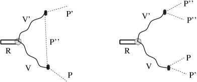
Figure 1: Resonance ($R$) decay to two (left) or four (right) pseudoscalar mesons ($P$, $P^{\prime}$, $P^{\prime\prime}$, $P^{\prime\prime\prime}$) through its $s$-wave (filled pattern hexagon) coupling to two vector mesons ($V$,$V^{\prime}$) and the $p$-wave coupling (black ovals) of these latter mesons to two pseudoscalar mesons.

A final remark is in order here. In our previous analysis carried out in Ref. GarciaRecio:2010ki , we also found two poles and made the same identifications as here. However in that work, we could not fine tune the subtraction constants to obtain masses for the second state below $1.75\,{\mathrm{GeV}}$. Thanks to the consideration of $\delta{\cal H}$ in the present analysis we have been able to predict two resonances with the appropriate masses to be identified with the $f_{2}(1270)$ and $f_{2}(1640)$ states. Nevertheless to achieve this, we have needed to use values of the subtraction constant of around $-3.9$. This in turn implies large UV cutoff values of around $3.5\,{\mathrm{GeV}}$, somehow in the limit of what one would expect for resonances dynamically generated by the unitarity loops driven by the LO potential. These large UV cutoffs might signal some resemblance between the nature of these states and that of the so called preexisting states, like the $\rho$ meson, for which higher order corrections (not driven by unitarity) in the potential play an important role in their dynamics Nieves:2009ez .

IV.3 Hypercharge 0, isospin 1 and spin 0

Table 3: Same as in Table 1, but for the $(Y,I,J)=(0,1,0)$ sector that corresponds to the $I^{G}(J^{PC})=1^{-}(0^{++})$ quantum numbers. The subtraction constants have been fixed to $a=-3.5$ in the $PP$ channels and to $a=-2.16$ in the $VV$ channels.

$(M_{R},\Gamma_{R})$	$\eta\pi$	$\bar{K}K$	$\omega\rho$	$\phi\rho$	$\bar{K}^{*}K^{*}$	$(M_{R},\Gamma_{R})$ GarciaRecio:2010ki	PDG $(M_{R},\Gamma_{R})$ Beringer:1900zz
$(970,90)$	2.67	2.82	7.33	2.62	0.09	$(990,92)$	$a_{0}(980)$	$(980\pm 20,50\sim 100)$
$(1493,86)$	1.68	2.26	2.04	8.24	8.08	$(1442,10)$	$a_{0}(1450)$	$(1474\pm 19,265\pm 13)$
						$(1760,24)$

There are five coupled channels in this sector: $\pi\eta$, $\bar{K}K$, $\rho\omega$, $\rho\phi$ and $\bar{K}^{*}K^{*}$ and we now find two poles in the SRS of the amplitudes. Our results are compiled in Table 3. The lowest pole should be identified with the $a_{0}(980)$, which has been obtained in all previous studies considering only pseudoscalar-pseudoscalar coupled channels. In our scheme, its couplings to the $\pi\eta$ and $K\bar{K}$ are large, in agreement with the results of earlier studies and with the data, but it also presents large couplings to the heaviest vector channels, $\omega\rho$ and $\phi\rho$. When comparing to the results of Ref. GarciaRecio:2010ki , we see that the couplings of this resonance to vector channels have drastically changed, though these heavier channels have little influence on the position of this lowest pole and on its allowed decay modes.

The pole at $(M_{R},\Gamma_{R})=(1493,86)\,{\mathrm{MeV}}$ can be naturally associated to the $a_{0}(1450)$ and its main features are similar to those found in GarciaRecio:2010ki . It decays to $\pi\eta$ and $K\bar{K}$, which is in agreement with the data. Its large couplings to the vector channels, whose thresholds are now closer, will give rise to new significant $\omega\pi\pi$ and $\bar{K}K\pi\pi$ decay modes, and to an important enhancement of its width thanks to the broad spectral functions of the $\rho$ and $K^{*}$ resonances.

Finally, as can be seen in the table, in our previous analysis of Ref. GarciaRecio:2010ki , we found a third pole, located at $(M_{R},\Gamma_{R})=(1760,24)\,{\mathrm{MeV}}$, and whose dynamics was mostly dominated by the vector channels. This further state could not be associated to any known state, since the PDG only reports two $a_{0}$ resonances below $2\,{\mathrm{GeV}}$. Nevertheless, in Ref. GarciaRecio:2010ki we suggested with some cautions that this third pole, though placed quite below, might be identified with the very broad $a_{0}(2020)$ resonance ($\Gamma=330\pm 75\,{\mathrm{MeV}}$). This latter resonance is not firmly established at all, and needs further confirmation. (Indeed, it appears in the section of Further states of the PDG.) In the present re-analysis, where the new spin symmetry breaking terms contained in $\delta{\cal H}$ have been included, this state is no longer dynamically generated.

IV.4 Hypercharge 0, isospin 1 and spin 2

Table 4: Same as in Table 1, but for the $(Y,I,J)=(0,1,2)$ sector that corresponds to the $I^{G}(J^{PC})=1^{-}(2^{++})$ quantum numbers. The subtraction constant has been set to $a=-3.88$ in all channels.

$(M_{R},\Gamma_{R})$	$\omega\rho$	$\phi\rho$	$\bar{K}^{*}K^{*}$	$(M_{R},\Gamma_{R})$ GarciaRecio:2010ki	PDG $(M_{R},\Gamma_{R})$ Beringer:1900zz
$(1319,0)$	8.41	1.92	5.32	$(1228,0)$	$a_{2}(1320)$	$(1318.3_{\mathrm{-0.6}}^{+0.5},107\pm 5)$
$(1747,12)$	1.55	3.48	4.82	$(1775,12)$	$a_{2}(1700)$	$(1732\pm 16,194\pm 40)$

There are three coupled channels in this sector: $\bar{K}^{*}K^{*}$, $\omega\rho$, and $\phi\rho$, and we find two poles, one in the FRS and the other one in the SRS of the amplitudes (see Table 4), which might be associated to the $a_{2}(1320)$ and $a_{2}(1700)$ resonances. The first state, bound in our model, couples strongly to the $\omega\rho$ channel, and its couplings would give rise to the observed $\pi\pi\pi$ and $\omega\pi\pi$ decay modes of the $a_{2}(1320)$ thanks to the width of the virtual $\rho$ meson. In our previous analysis GarciaRecio:2010ki , we could not place the mass of this state above $1230\,{\mathrm{MeV}}$, despite we tried some fine-tuning of the subtraction constants. Thus here, as it was also the case in the $(Y,I,J)=(0,0,2)$ sector, we find a better overall description of the sector thanks to the inclusion of the $\delta{\cal H}$ terms.

The $a_{2}(1320)$ resonance is not dynamically generated in the hidden gauge model of Ref. Geng:2008gx , though there it is reported one state whose features are similar to those of the second (heaviest) pole found here. This second pole might be associated to the $a_{2}(1700)$, since its mass and expected decays into $\omega\rho$, $\omega\pi^{-}\pi^{0}$ and $K\bar{K}$ (from the decays into virtual $\phi\rho$ or $K^{*}\bar{K}^{*}$ pairs) are in good agreement with the information listed in the PDG for the $a_{2}(1700)$ resonance. However, the state predicted here, as it was the case in Refs. GarciaRecio:2010ki ; Geng:2008gx turns out to be much narrower than this resonance. This is probably an indication that other mechanisms, such as coupled-channel $d$-wave dynamics, might play an important role in this case. Nevertheless, there exists a large uncertainty in the experimental status of the $a_{2}(1700)$.

Finally, we should point out here that in this sector, we have also needed to make use of large UV cutoffs ($\sim 3.5\,{\mathrm{GeV}}$), somehow in the limit of what one would expect for resonances dynamically generated by the unitarity loops driven by the LO potential.

IV.5 Hypercharge 1, isospin 1/2 and spin 0

In this sector we find three poles, with positions and couplings compiled in Table 5. There we have also collected the pole positions found in our previous work of Ref. GarciaRecio:2010ki . Masses and widths listed in the PDG Beringer:1900zz of the possible resonances that could be identified with these states are also given in the table. As in the $(Y,I,J)=(0,0,0)$ sector, the inclusion of $\delta{\cal H}$ in the present work has very little effect, and the present results are quite similar to those already obtained in GarciaRecio:2010ki . Again, we refer to that work for further details and grounds on the identification proposed in Table 5. Very briefly, it looks quite natural to identify the first two poles with the PDG $K^{*}_{0}(800)$ and $K^{*}_{0}(1430)$ states, in spite of being the latter one much wider than the pole found in our scheme. The $K\pi$ branching fraction for this resonance is $93\%\pm 10\%$. For our pole at $1425\,{\mathrm{MeV}}$, the direct coupling to $K\pi$ is not so dominant over the other open channel, $\eta K$. However, the couplings to the closed channels $K^{*}\rho$, $K^{*}\omega$, $K^{*}\phi$ channels are much larger. As a consequence, the resonance can decay into a virtual $K^{*}\rho$ pair and significantly enhance the $K\pi$ decay probability, through the loop mechanism depicted in the left panel of Fig. 1, thanks to the broad $\rho$ and $K^{*}$ spectral functions.

The identification of the third pole with the broad $K^{*}_{0}(1950)$ resonance is less straightforward. Nevertheless, it should be pointed out that the $K^{*}_{0}(1950)$ resonance is not firmly established yet and needs further confirmation Beringer:1900zz .

A final comment is related with the employed UV cutoffs in this sector. Those turn out to be of the order of $1\,{\mathrm{GeV}}$ in this case, as it was also the case in the $(Y,I,J)=(0,0,0)$ sector, indicating that the dynamics of the resonances in both sectors are mostly governed by the logs that appear in the unitarity loops. This naturally explains why, for instance, the $K^{*}_{0}(800)$ is so wide, since it is placed well above the relevant threshold $K\pi$. Indeed, this resonance is very similar to the $f_{0}(500)$, and it cannot be interpreted as a Breit-Wigner narrow resonance.

Table 5: Same as in Table 1, but for the $(Y,I,J)=(1,1/2,0)$ sector that corresponds to the $I(J^{P})=\frac{1}{2}(0^{+})$ quantum numbers. The subtraction constant has been set to $a=-1.52$ in all channels. The assignment of the third pole to the $K^{*}_{0}(1950)$ resonance is uncertain.

$(M_{R},\Gamma_{R})$	$K\pi$	$\eta K$	$K^{*}\rho$	$K^{*}\omega$	$K^{*}\phi$	$(M_{R},\Gamma_{R})$ GarciaRecio:2010ki	PDG $(M_{R},\Gamma_{R})$ Beringer:1900zz
$(816,434)$	4.83	2.20	6.29	2.29	2.15	$(812,347)$	$K^{*}_{0}(800)$	$(682\pm 29,547\pm 24)$
$(1425,54)$	1.91	1.02	8.11	10.69	5.70	$(1428,48)$	$K^{*}_{0}(1430)$	$(1425\pm 50,270\pm 80)$
$(1782,90)$	0.06	2.92	0.68	1.07	12.21	$(1787,74)$	$K^{*}_{0}(1950)$	$(1945\pm 22,201\pm 90)$

IV.6 Hypercharge 1, isospin 1/2 and spin 2

Table 6: Same as in Table 1, but for the $(Y,I,J)=(1,1/2,2)$ sector that corresponds to the $I(J^{P})=\frac{1}{2}(2^{+})$ quantum numbers. The subtraction constant has been set to $a=-4.32$ in all channels. The assignment of the second pole to the $K^{*}_{2}(1980)$ resonance is uncertain.

$(M_{R},\Gamma_{R})$	$K^{*}\rho$	$K^{*}\omega$	$K^{*}\phi$	$(M_{R},\Gamma_{R})$ GarciaRecio:2010ki	PDG $(M_{R},\Gamma_{R})$ Beringer:1900zz
$(1430,0)$	6.30	4.23	6.81	$(1701,313)$	$K^{*}_{2}(1430)$	$(1429\pm 4,104\pm 6)$
$(1624,0)$	6.21	0.39	2.88		$K^{*}_{2}(1980)$	$(1973\pm 26,373\pm 70)$

In this sector (Table 6), we find two poles in the FRS/SRS of the amplitudes. In the PDG, two $K^{*}_{2}$ resonances [$K^{*}_{2}(1430)$ and $K^{*}_{2}(1980)$] are reported below $2\,{\mathrm{GeV}}$ Beringer:1900zz , though only the lightest one is firmly established. In the analysis of Ref. GarciaRecio:2010ki just one state was found, and moreover, the subtraction constants could not be fine-tuned to bring its mass below $1.7\,{\mathrm{GeV}}$. The consideration of $\delta{\cal H}$ in the current approach overcomes this problem, and it allows to generate a pole in the region of $1430\,{\mathrm{MeV}}$. According to the PDG, the $K^{*}_{2}(1430)$ has a width of $104\pm 6\,{\mathrm{MeV}}$, in our approach we find a bound state, located below all the thresholds. The PDG branching fractions are around 50%, 25%, 9% and 3% for the $D$-wave modes $K\pi$, $K^{*}\pi$, $K\rho$ and $K\omega$, respectively. In addition, the branching fraction of the $K^{*}\pi\pi$ channel is only about 13%. Certainly, these modes can be also originated from the decay of the resonance to $K^{*}\rho$, $K^{*}\omega$ and $K^{*}\phi$ virtual pairs. In particular, we expect the $K^{*}\rho$ channel to play an important role, because of the broad spectral functions of both the $K^{*}$ and $\rho$ mesons and its proximity to the mass of the resonance, since it can trigger a significant part of the observed $K^{*}_{2}(1430)$ decays into $K\pi$ and $K^{*}\pi\pi$ (see Fig. 1). Note that the large $K^{*}\phi$ coupling also provides a contribution to the dominant $K\pi$ mode.

We should note, however, that we need to use values of the subtraction constants that amount to UV cutoffs above $4\,{\mathrm{GeV}}$, which put some doubts on the real nature of this state, as we discussed in $(Y,I,J)=$(0,0,2) and (0,1,2) sectors. It might be the case that large UV cutoffs are needed to compensate the genuine (non resonant driven) $D$-wave channels ignored in the present coupled channels approach. In particular, in Ref. GarciaRecio:2010ki it was already pointed out the possible influence of the $D$-wave pseudoscalar-vector meson $K^{*}\pi$ channel, which lies closer to the resonance mass than the pseudoscalar-pseudoscalar channels.

The hidden gauge approach of Ref. Geng:2008gx for $VV\to VV$ scattering produces a resonance in this sector, with mass fine-tuned to $1430\,{\mathrm{MeV}}$, and properties quite similar to those found here. There, all $D$-wave type interactions were also ignored.

On the other hand, little is known about the $K_{2}^{*}(1980)$, and the assignment of our second pole to this resonance is clearly uncertain. (Note that in Ref. GarciaRecio:2010ki , a second pole was not generated in this sector.) The large width of this state ($\Gamma\sim 400$) makes less meaningful the difference between its mass and that of our pole, which might be then associated to this resonance. Still, it should be noted again that the $K_{2}^{*}(1980)$ resonance is not yet firmly established and needs further confirmation. It might well happen that the pole obtained here corresponds to a different state not yet detected.

IV.7 Exotics

Table 7: Same as in Table 1, but for the $(Y,I,J)=(0,2,0)$ sector that corresponds to the exotic $I^{G}(J^{PC})=2^{+}(0^{++})$ quantum numbers. The subtraction constant has been set to $a=-1.51$ in all channels.

$(M_{R},\Gamma_{R})$	$\pi\pi$	$\rho\rho$	$(M_{R},\Gamma_{R})$ GarciaRecio:2010ki	PDG $(M_{R},\Gamma_{R})$ Beringer:1900zz
$(1420,110)$	2.74	9.99	$(1418,108)$	$X(1420)$	$(1420\pm 20,160\pm 10)$

Exotics refers here to meson states with quantum numbers that cannot be formed by a $q\bar{q}$ pair. Quantum numbers with $I>1$ or $|Y|>1$ are exotic.

Besides the exotic poles with $J=1$ in the sectors $(Y=1,I=3/2)$ and $(Y=2,I=0)$ already reported in Ref. GarciaRecio:2010ki , we find another three exotic states with $J=0$ in region $1.4-1.6\,{\mathrm{GeV}}$. Their positions and couplings are compiled in Tables 7, 8 and 9. In these tables, we have also collected the pole positions found in Ref. GarciaRecio:2010ki . These scalar exotic states appear in the sectors $(Y=0,I=2)$, $(Y=1,I=3/2)$ and $(Y=2,I=1)$. As already pointed out in Ref. GarciaRecio:2010ki , the matrices ${\mathcal{D}}_{\rm kin}$ and ${\mathcal{D}}_{m}$ in Eq. (20) are identical in the three sectors. The analogous statement holds for the new interactions ${\mathcal{D}}_{2}$ and ${\mathcal{D}}_{3}$ (Eq. (21)). Thus, clearly the three spin zero exotic states are just related by flavor rotations.

Table 8: Same as in Table 1, but for the $(Y,I,J)=(1,3/2,0)$ sector that corresponds to the exotic $I(J^{P})=\frac{3}{2}(0^{+})$ quantum numbers. The subtraction constant has been set to $a=-2.0$ in all channels.

$(M_{R},\Gamma_{R})$	$K\pi$	$K^{*}\rho$	$(M_{R},\Gamma_{R})$ GarciaRecio:2010ki
$(1438,140)$	3.26	10.86	$(1431,140)$

As in the $(Y,I,J)=(0,0,0)$ and $(Y,I,J)=(1,1/2,0)$ sectors, the inclusion of $\delta{\cal H}$ in the present work has very little effect and the present results are quite similar (practically identical) to those already obtained in GarciaRecio:2010ki . We refer to that work for further details as well as for an overall picture of the poles with exotic quantum numbers predicted for this SU(6) extension of the WT Lagrangian. In short, there is only state listed in the PDG that can be associated with the exotic resonances predicted by our model. This is the $X(1420)$ resonance, but it needs further confirmation and its current evidence comes from a statistical indication Filippi:2000is for a $\pi^{+}\pi^{+}$ resonant state in the $\bar{n}p\to\pi^{+}\pi^{+}\pi^{-}$ annihilation reaction with data collected by the OBELIX experiment. In our model, the pole is mainly a $\rho\rho$ bound state with a small coupling to the $\pi\pi$ channel that moves the pole to the SRS. Within our scheme, the $\rho\rho\to\rho\rho$ amplitude is totally symmetric under $I\leftrightarrow J$ exchange. As a consequence our $\rho\rho$ potential in this sector ($I=2,J=0$) is the same as that in the $I=0,J=2$ one. BSE amplitudes in both sectors will become different because of coupled-channel and renormalization effects. Nevertheless, we expect the $X(1420)$ to be the counterpart of the $f_{2}(1270)$, which appeared with a large $\rho\rho$ spin two isoscalar component. As mentioned, the other two spin zero exotic states in the $(Y=1,I=3/2)$ and $(Y=2,I=1)$ sectors should be related to $X(1420)$ by a flavor rotation. However, there is no experimental evidence of their existence yet.

Table 9: Same as in Table 1, but for the $(Y,I,J)=(2,1,0)$ sector that corresponds to the exotic $I(J^{P})=1(0^{+})$ quantum numbers. The subtraction constant has been set to $a=-2.0$ in all channels.

$(M_{R},\Gamma_{R})$	$\bar{K}K$	$\bar{K^{*}}K^{*}$	$(M_{R},\Gamma_{R})$ GarciaRecio:2010ki
$(1568,132)$	3.50	11.49	$(1563,132)$

Finally, we just mention that the ${\mathcal{D}}_{\rm kin}$, ${\mathcal{D}}_{m}$, ${\mathcal{D}}_{2}$ and ${\mathcal{D}}_{3}$ matrices are identical in the three sectors $(Y,I,J)=(0,2,2),(1,3/2,2)$ and $(2,1,2)$. They provide a repulsive interaction and hence no resonance is predicted in those exotic sectors by our model.

V Summary

We have reviewed the model presented in Ref. GarciaRecio:2010ki to address the dynamics of the low-lying even parity meson resonances. It is based on a spin-flavor extension of the chiral WT Lagrangian, which is then used to study the $S$-wave meson-meson interaction involving members not only of the $\pi$-octet, but also of the $\rho$-nonet. Elastic unitarity in coupled channels is restored by solving a renormalized coupled channels BSE, and a certain pattern of SU(6) spin–flavor symmetry breaking is implemented. The model probed to be phenomenologically successful in the $J^{P}=0^{+}$ and $1^{+}$ sectors. Actually in  GarciaRecio:2010ki , it was shown that most of the low-lying even parity PDG meson resonances in these two spin sectors could be classified according to multiplets of SU(6). However the scheme of Ref. GarciaRecio:2010ki is not so successful for the sectors with spin 2. It fails to appropriately describe some well established $J^{P}=2^{+}$ resonances, like the $K^{*}_{2}(1430)$, that in the hidden gauge formalism for vector mesons used in Ref. Geng:2008gx are dynamically generated in a natural manner. In this work, we have improved on that by supplementing the model of Ref. GarciaRecio:2010ki with new local $VV$ interactions consistent with CS.

To provide different pseudoscalar and vector mesons masses, a simple spin-symmetry breaking local term that preserved CS was designed in  GarciaRecio:2010ki . Here, we have studied in detail the structure of the SU(6) symmetry breaking local terms that respect (or softly break) CS. Thus, in this work, we have derived the most general contact terms consistent with the chiral symmetry breaking pattern of QCD as expressed in terms of the field $U$. We have also shown that there is a finite number of chirally invariant contact four meson-field interactions, restricted also by the other symmetries of the problem. To reduce the number of parameters to a manageable size, and in the spirit of large $N_{C}$, we have restricted our analysis to interactions involving just one trace.

Further, we have carried out a phenomenological discussion of the effects of these new terms. We find that their inclusion leads to a considerable improvement of the description of the $J^{P}=2^{+}$ sector, without spoiling the main features of the predictions obtained in Ref. GarciaRecio:2010ki for the $J^{P}=0^{+}$ and $J^{P}=1^{+}$ sectors. In particular, we have found a significantly better description of the $I^{G}(J^{PC})=0^{+}(2^{++})$, $1^{-}(2^{++})$ and the $I(J^{P})=\frac{1}{2}(2^{+})$ sectors, that correspond to the $f_{2}(1270)$, $a_{2}(1320)$ and $K^{*}_{2}(1430)$ quantum numbers, respectively. Besides the position of the resonances, we also estimate the couplings of those resonances to the different channels, which is relevant to describe the state structure and its favored decay modes. Our analysis shows that $2^{+}$ states systematically require cutoff values which lie in the boundary of their natural hadronic domain. This could be an indication that $D$-wave mechanisms play some role in the formation of such states. The fact that, in many cases, the thresholds of the main channels are not too close to the resonance position, also suggests that pure $S$-wave interactions would not necessarily saturate the formation mechanisms of those resonances. Of course, for some particular mesonic resonances, it could also be the case that they are mostly genuine rather than dynamically generated. With this possible caveat in mind, we can say that the model produces a rather robust and successful scheme to study the low-lying even parity resonances that are dynamically generated by the logs that appear in the unitarity loops.

Appendix A Chiral invariant four meson interaction with a single trace

In this appendix we show that, the operators $\mathcal{O}_{1}$, $\mathcal{O}_{2}$, $\mathcal{O}_{3}$ in Eq. (13), already saturate the most general chiral invariant interaction, modulo $O(\Phi_{6}^{6})$, stemming from single trace Lagrangian terms.

Rather than doing the expansion of the most general term ${\mathrm{tr}}(\mathcal{U}_{ij}\mathcal{U}_{kl}\cdots)$ in powers of the meson field, we just write down the possible operators in terms of the meson field and seek the most general combination invariant under infinitesimal chiral rotations. To alleviate the notation, we use $U_{6}=e^{\phi}$, $\phi$ being antihermitian and dimensionless. This is related with the usual meson field by $\phi=2i\Phi_{6}/f$.

The 8 possible terms, assuming other symmetries but not chiral invariance, are as follows

$$A_{1} = {\mathrm{tr}}(\phi^{2}),$$

$$A_{2} = {\mathrm{tr}}(\sigma_{i}\phi\sigma_{i}\phi),$$

$$A_{3} = {\mathrm{tr}}(\phi^{4}),$$

$$A_{4} = {\mathrm{tr}}(\sigma_{i}\phi\sigma_{i}\phi^{3}),$$

$$A_{5} = {\mathrm{tr}}(\sigma_{i}\phi^{2}\sigma_{i}\phi^{2}),$$

$$A_{6} = i\epsilon_{ijk}{\mathrm{tr}}(\sigma_{i}\phi\sigma_{j}\phi\sigma_{k}\phi^{2}),$$

$$A_{7} = {\mathrm{tr}}(\sigma_{i}\phi\sigma_{i}\phi\sigma_{j}\phi\sigma_{j}\phi),$$

$$A_{8} = {\mathrm{tr}}(\sigma_{i}\phi\sigma_{j}\phi\sigma_{i}\phi\sigma_{j}\phi).$$ (25)

The operators $A_{1}$ and $A_{2}$ give mass to the mesons, the other provide interaction.

Under a chiral rotation $U_{6}\to\Omega_{L}^{\dagger}U_{6}\Omega_{R}$, and this induces a non linear transformation on $\phi$. Vector invariance ($\Omega_{L}=\Omega_{R}$) is a similarity transformation which produces the same transformation on $\phi$ and it is trivially satisfied by the 8 operators. Therefore we consider just axial transformations $\Omega_{L}=\Omega_{R}^{\dagger}$. Only infinitesimal transformations are needed, $\Omega_{R}=e^{\delta\alpha/2}=1+\frac{1}{2}\delta\alpha$, with $\delta\alpha$ infinitesimal, antihermitian and spinless. This induces the transformation

$$\delta\phi=\delta\alpha+\frac{1}{12}\delta\alpha\phi^{2}+\frac{1}{12}\phi^{2}\delta\alpha-\frac{1}{6}\phi\delta\alpha\phi+O(\phi^{4}).$$ (26)

(To all orders in the meson field, the infinitesimal axial variation contains only even powers of $\phi$.)

The variations of $A_{1}$ and $A_{2}$ produce terms of $O(\phi)$ that can only be canceled by choosing a suitable combination of the two operators. Also they produce terms of $O(\phi^{3})$. They should cancel with the corresponding variations from the quartic terms, taking suitable combinations of them. The cancellation to order $O(\phi^{5})$ is of no concern to us as this involves $O(\phi^{6})$ interactions. The cancellation will be automatic for the expansion of any of the terms ${\mathrm{tr}}(\mathcal{U}_{ij}\mathcal{U}_{kl}\cdots)$ since chiral invariance is manifest in those terms.

For a generic operator $H=\sum_{i=1}^{8}c_{i}A_{i}$, the condition $\delta H=O(\phi^{5})$ gives the following conditions

$$0 = 2c_{1}+6c_{2},$$

$$0 = 4c_{3}+3c_{4},$$

$$0 = -\frac{1}{3}c_{2}+c_{4}+8c_{7}+4c_{8},$$

$$0 = \frac{1}{6}c_{2}+c_{4}+2c_{5}-2c_{6},$$

$$0 = \frac{1}{6}c_{2}+c_{4}+2c_{5}-2c_{6},$$

$$0 = 2c_{6}-2c_{7}+4c_{8}.$$ (27)

They correspond, respectively, to the vanishing of the coefficients of ${\mathrm{tr}}(\phi\delta\alpha)$, ${\mathrm{tr}}(\phi^{3}\delta\alpha)$, ${\mathrm{tr}}(\phi\sigma_{i}\phi\sigma_{i}\phi\delta\alpha)$, ${\mathrm{tr}}(\sigma_{i}\phi\sigma_{i}\phi^{2}\delta\alpha)$, ${\mathrm{tr}}(\sigma_{i}\phi^{2}\sigma_{i}\phi\delta\alpha)$, and $i\epsilon_{ijk}{\mathrm{tr}}(\sigma_{i}\phi\sigma_{j}\phi\sigma_{k}\phi\delta\alpha)$.

The 5 independent relations leave 3 chiral invariant combinations. They can be taken as

$$H_{\mathrm{inv}}=c_{1}(A_{1}-\frac{1}{3}A_{2}-\frac{1}{36}A_{6}-\frac{1}{60}A_{7}+\frac{1}{180}A_{8})+c_{3}(A_{3}-\frac{4}{3}A_{4}-\frac{2}{3}A_{6}+\frac{1}{3}A_{8})+c_{5}(A_{5}+A_{6}+\frac{1}{5}A_{7}-\frac{2}{5}A_{8}).$$ (28)

The three combinations $\mathcal{O}_{1}$, $(\mathcal{O}_{2}-20\mathcal{O}_{1})/12$, and $\mathcal{O}_{3}/3$ in Section III correspond, respectively, to $(c_{1},c_{3},c_{5})=(3,\frac{1}{4},\frac{1}{4})$, $(0,1,\frac{5}{6})$, and $(0,1,0)$.

Appendix B Coefficients of the $S$-wave tree level amplitudes

This Appendix gives the ${\mathcal{D}}_{2}$ and ${\mathcal{D}}_{3}$ matrices of the $S$-wave tree level meson-meson amplitudes in Eq. (21), for the various $YIJ$ sectors (Tables 10-47). Note that for the $Y=0$ channels, $G$-parity is conserved, and that all $Y=0$ states have well-defined $G$-parity except the $\bar{K}^{*}K$ and $K^{*}\bar{K}$ states, but the combinations $\left(\bar{K}K^{*}\pm K\bar{K}^{*}\right)/\sqrt{2}$ are actually $G$-parity eigenstates with eigenvalues $\pm 1$. These states will be denoted $(\bar{K}K^{*})_{S}$ and $(\bar{K}K^{*})_{A}$, respectively.

B.1 ${\mathcal{D}}_{2}$

Table 10: $(Y,I,J)=(0,0,0)$.

	$\pi\pi$	$\bar{K}K$	$\eta\eta$	$\rho\rho$	$\omega\omega$	$\omega\phi$	$\bar{K}^{*}K^{*}$	$\phi\phi$
	0	0	0	0	0	0	0	0
	0	0	0	0	0	0	0	0
	0	0	0	0	0	0	0	0
	0	0	0	$-\frac{208}{3}$	$\frac{80}{\sqrt{3}}$	0	$24\sqrt{3}$	0
	0	0	0	$\frac{80}{\sqrt{3}}$	$-\frac{80}{3}$	0	$-24$	0
	0	0	0	0	0	0	$\frac{16}{3}$	0
	0	0	0	$24\sqrt{3}$	$-24$	$\frac{16}{3}$	$-72$	$-48$
	0	0	0	0	0	0	$-48$	$-\frac{160}{3}$

Table 11: $(Y,I,J)=(0,0,1)$.

$G$	$\eta\phi$	$\eta\omega$	$\pi\rho$	$(\bar{K}K^{*})_{A}$	$\bar{K}^{*}K^{*}$	$\omega\phi$	$(\bar{K}K^{*})_{S}$
$-$	0	0	0	0	0
$-$	0	0	0	0	0
$-$	0	0	0	0	0
$-$	0	0	0	0	0
$-$	0	0	0	0	$-28$
$+$						0	0
$+$						0	0

Table 12: $(Y,I,J)=(0,0,2)$.

	$\rho\rho$	$\omega\omega$	$\omega\phi$	$\bar{K}^{*}K^{*}$	$\phi\phi$
	$-\frac{16}{3}$	$\frac{32}{\sqrt{3}}$	0	$4\sqrt{3}$	0
	$\frac{32}{\sqrt{3}}$	$-\frac{32}{3}$	0	$-4$	0
	0	0	0	$\frac{40}{3}$	0
	$4\sqrt{3}$	$-4$	$\frac{40}{3}$	$-12$	$-8$
	0	0	0	$-8$	$-\frac{64}{3}$

Table 13: $(Y,I,J)=(0,1,0)$.

	$\eta\pi$	$\bar{K}K$	$\omega\rho$	$\phi\rho$	$\bar{K}^{*}K^{*}$
	0	0	0	0	0
	0	0	0	0	0
	0	0	$-\frac{160}{3}$	0	$24\sqrt{2}$
	0	0	0	0	$-\frac{16}{3}$
	0	0	$24\sqrt{2}$	$-\frac{16}{3}$	$-24$

Table 14: $(Y,I,J)=(0,1,1)$.

$G$	$\pi\phi$	$\pi\omega$	$\eta\rho$	$(\bar{K}K^{*})_{S}$	$\rho\rho$	$\bar{K}^{*}K^{*}$	$\pi\rho$	$(\bar{K}K^{*})_{A}$	$\omega\rho$	$\phi\rho$
$+$	0	0	0	0	0	0
$+$	0	0	0	0	0	0
$+$	0	0	0	0	0	0
$+$	0	0	0	0	0	0
$+$	0	0	0	0	$-\frac{56}{3}$	$\frac{28\sqrt{2}}{3}$
$+$	0	0	0	0	$\frac{28\sqrt{2}}{3}$	$-\frac{28}{3}$
$-$							0	0	0	0
$-$							0	0	0	0
$-$							0	0	0	0
$-$							0	0	0	0

Table 15: $(Y,I,J)=(0,1,2)$.

	$\omega\rho$	$\phi\rho$	$\bar{K}^{*}K^{*}$
	$-\frac{64}{3}$	0	$4\sqrt{2}$
	0	0	$-\frac{40}{3}$
	$4\sqrt{2}$	$-\frac{40}{3}$	$-4$

Table 16: $(Y,I,J)=(0,2,0)$.

	$\pi\pi$	$\rho\rho$
	0	0
	0	$-\frac{16}{3}$

Table 17: $(Y,I,J)=(0,2,1)$.

	$\pi\rho$
	0

Table 18: $(Y,I,J)=(0,2,2)$.

	$\rho\rho$
	$-\frac{40}{3}$

Table 19: $(Y,I,J)=(1,1/2,0)$.

	$K\pi$	$\eta K$	$K^{*}\rho$	$K^{*}\omega$	$K^{*}\phi$
	0	0	0	0	0
	0	0	0	0	0
	0	0	$-\frac{100}{3}$	$-\frac{44}{\sqrt{3}}$	$12\sqrt{6}$
	0	0	$-\frac{44}{\sqrt{3}}$	$-\frac{44}{3}$	$12\sqrt{2}$
	0	0	$12\sqrt{6}$	$12\sqrt{2}$	$-\frac{88}{3}$

Table 20: $(Y,I,J)=(1,1/2,1)$.

	$\pi K^{*}$	$K\rho$	$K\omega$	$\eta K^{*}$	$K\phi$	$K^{*}\rho$	$K^{*}\omega$	$K^{*}\phi$
	0	0	0	0	0	0	0	0
	0	0	0	0	0	0	0	0
	0	0	0	0	0	0	0	0
	0	0	0	0	0	0	0	0
	0	0	0	0	0	0	0	0
	0	0	0	0	0	$-14$	$-\frac{14}{\sqrt{3}}$	$-14\sqrt{\frac{2}{3}}$
	0	0	0	0	0	$-\frac{14}{\sqrt{3}}$	$-\frac{14}{3}$	$-\frac{14\sqrt{2}}{3}$
	0	0	0	0	0	$-14\sqrt{\frac{2}{3}}$	$-\frac{14\sqrt{2}}{3}$	$-\frac{28}{3}$

Table 21: $(Y,I,J)=(1,1/2,2)$.

	$K^{*}\rho$	$K^{*}\omega$	$K^{*}\phi$
	$\frac{2}{3}$	$-\frac{26}{\sqrt{3}}$	$2\sqrt{6}$
	$-\frac{26}{\sqrt{3}}$	$-\frac{26}{3}$	$2\sqrt{2}$
	$2\sqrt{6}$	$2\sqrt{2}$	$-\frac{52}{3}$

Table 22: $(Y,I,J)=(1,3/2,0)$.

	$K\pi$	$K^{*}\rho$
	$0$	0
	0	$-\frac{16}{3}$

Table 23: $(Y,I,J)=(1,3/2,1)$.

	$\pi K^{*}$	$K\rho$	$K^{*}\rho$
	0	0	0
	0	0	0
	0	0	0

Table 24: $(Y,I,J)=(1,3/2,2)$.

	$K^{*}\rho$
	$-\frac{40}{3}$

Table 25: $(Y,I,J)=(2,0,1)$.

	$KK^{*}$	$K^{*}K^{*}$
	0	0
	0	0

Table 26: $(Y,I,J)=(2,1,0)$.

	$KK$	$K^{*}K^{*}$
	$0$	$0$
	$0$	$-\frac{16}{3}$

Table 27: $(Y,I,J)=(2,1,1)$.

	$KK^{*}$
	$0$

Table 28: $(Y,I,J)=(2,1,2)$.

	$K^{*}K^{*}$
	$-\frac{40}{3}$

B.2 ${\mathcal{D}}_{3}$

Table 29: $(Y,I,J)=(0,0,0)$.

	$\pi\pi$	$\bar{K}K$	$\eta\eta$	$\rho\rho$	$\omega\omega$	$\omega\phi$	$\bar{K}^{*}K^{*}$	$\phi\phi$
	0	0	0	0	0	0	0	0
	0	0	0	0	0	0	0	0
	0	0	0	0	0	0	0	0
	0	0	0	$-\frac{128}{3}$	0	0	$\frac{32}{\sqrt{3}}$	0
	0	0	0	0	0	0	$-\frac{32}{3}$	0
	0	0	0	0	0	0	$-\frac{64}{3}$	0
	0	0	0	$\frac{32}{\sqrt{3}}$	$-\frac{32}{3}$	$-\frac{64}{3}$	$-32$	$-\frac{64}{3}$
	0	0	0	0	0	0	$-\frac{64}{3}$	0

Table 30: $(Y,I,J)=(0,0,1)$.

$G$	$\eta\phi$	$\eta\omega$	$\pi\rho$	$(\bar{K}K^{*})_{A}$	$\bar{K}^{*}K^{*}$	$\omega\phi$	$(\bar{K}K^{*})_{S}$
$-$	0	0	0	0	0
$-$	0	0	0	0	0
$-$	0	0	0	0	0
$-$	0	0	0	0	0
$-$	0	0	0	0	$-48$
$+$						0	0
$+$						0	0

Table 31: $(Y,I,J)=(0,0,2)$.

	$\rho\rho$	$\omega\omega$	$\omega\phi$	$\bar{K}^{*}K^{*}$	$\phi\phi$
	$\frac{64}{3}$	0	0	$-\frac{16}{\sqrt{3}}$	0
	0	0	0	$\frac{16}{3}$	0
	0	0	0	$\frac{32}{3}$	0
	$-\frac{16}{\sqrt{3}}$	$\frac{16}{3}$	$\frac{32}{3}$	$16$	$\frac{32}{3}$
	0	0	0	$\frac{32}{3}$	0

Table 32: $(Y,I,J)=(0,1,0)$.

	$\eta\pi$	$\bar{K}K$	$\omega\rho$	$\phi\rho$	$\bar{K}^{*}K^{*}$
	0	0	0	0	0
	0	0	0	0	0
	0	0	0	0	$\frac{32\sqrt{2}}{3}$
	0	0	0	0	$\frac{64}{3}$
	0	0	$\frac{32\sqrt{2}}{3}$	$\frac{64}{3}$	$-\frac{32}{3}$

Table 33: $(Y,I,J)=(0,1,1)$.

$G$	$\pi\phi$	$\pi\omega$	$\eta\rho$	$(\bar{K}K^{*})_{S}$	$\rho\rho$	$\bar{K}^{*}K^{*}$	$\pi\rho$	$(\bar{K}K^{*})_{A}$	$\omega\rho$	$\phi\rho$
$+$	0	0	0	0	0	0
$+$	0	0	0	0	0	0
$+$	0	0	0	0	0	0
$+$	0	0	0	0	0	0
$+$	0	0	0	0	$-32$	$16\sqrt{2}$
$+$	0	0	0	0	$16\sqrt{2}$	$-16$
$-$							0	0	0	0
$-$							0	0	0	0
$-$							0	0	0	0
$-$							0	0	0	0

Table 34: $(Y,I,J)=(0,1,2)$.

	$\omega\rho$	$\phi\rho$	$\bar{K}^{*}K^{*}$
	0	0	$-\frac{16\sqrt{2}}{3}$
	0	0	$-\frac{32}{3}$
	$-\frac{16\sqrt{2}}{3}$	$-\frac{32}{3}$	$\frac{16}{3}$

Table 35: $(Y,I,J)=(0,2,0)$.

	$\pi\pi$	$\rho\rho$
	0	0
	0	$\frac{64}{3}$

Table 36: $(Y,I,J)=(0,2,1)$.

	$\pi\rho$
	0

Table 37: $(Y,I,J)=(0,2,2)$.

	$\rho\rho$
	$-\frac{32}{3}$

Table 38: $(Y,I,J)=(1,1/2,0)$.

	$K\pi$	$\eta K$	$K^{*}\rho$	$K^{*}\omega$	$K^{*}\phi$
	0	0	0	0	0
	0	0	0	0	0
	0	0	$-\frac{80}{3}$	$\frac{16}{\sqrt{3}}$	$16\sqrt{\frac{2}{3}}$
	0	0	$\frac{16}{\sqrt{3}}$	$\frac{16}{3}$	$\frac{16\sqrt{2}}{3}$
	0	0	$16\sqrt{\frac{2}{3}}$	$\frac{16\sqrt{2}}{3}$	$\frac{32}{3}$

Table 39: $(Y,I,J)=(1,1/2,1)$.

	$\pi K^{*}$	$K\rho$	$K\omega$	$\eta K^{*}$	$K\phi$	$K^{*}\rho$	$K^{*}\omega$	$K^{*}\phi$
	0	0	0	0	0	0	0	0
	0	0	0	0	0	0	0	0
	0	0	0	0	0	0	0	0
	0	0	0	0	0	0	0	0
	0	0	0	0	0	0	0	0
	0	0	0	0	0	$-24$	$-8\sqrt{3}$	$-8\sqrt{6}$
	0	0	0	0	0	$-8\sqrt{3}$	$-8$	$-8\sqrt{2}$
	0	0	0	0	0	$-8\sqrt{6}$	$-8\sqrt{2}$	$-16$

Table 40: $(Y,I,J)=(1,1/2,2)$.

	$K^{*}\rho$	$K^{*}\omega$	$K^{*}\phi$
	$\frac{40}{3}$	$-\frac{8}{\sqrt{3}}$	$-8\sqrt{\frac{2}{3}}$
	$-\frac{8}{\sqrt{3}}$	$-\frac{8}{3}$	$-\frac{8\sqrt{2}}{3}$
	$-8\sqrt{\frac{2}{3}}$	$-\frac{8\sqrt{2}}{3}$	$-\frac{16}{3}$

Table 41: $(Y,I,J)=(1,3/2,0)$.

	$K\pi$	$K^{*}\rho$
	$0$	0
	0	$\frac{64}{3}$

Table 42: $(Y,I,J)=(1,3/2,1)$.

	$\pi K^{*}$	$K\rho$	$K^{*}\rho$
	0	0	0
	0	0	0
	0	0	0

Table 43: $(Y,I,J)=(1,3/2,2)$.

	$K^{*}\rho$
	$-\frac{32}{3}$

Table 44: $(Y,I,J)=(2,0,1)$.

	$KK^{*}$	$K^{*}K^{*}$
	0	0
	0	0

Table 45: $(Y,I,J)=(2,1,0)$.

	$KK$	$K^{*}K^{*}$
	$0$	$0$
	$0$	$\frac{64}{3}$

Table 46: $(Y,I,J)=(2,1,1)$.

	$KK^{*}$
	$0$

Table 47: $(Y,I,J)=(2,1,2)$.

	$K^{*}K^{*}$
	$-\frac{32}{3}$

References

- (1) A. Bondar et al. [Belle Collaboration], Phys. Rev. Lett. 108 (2012) 122001.
- (2) S. K. Choi et al. [Belle Collaboration], Phys. Rev. Lett. 91 (2003) 262001.
- (3) J. Vijande, A. Valcarce and J. -M. Richard, Phys. Rev. D 76 (2007) 114013.
- (4) P. G. Ortega, J. Segovia, D. R. Entem and F. Fernandez, Phys. Rev. D 81 (2010) 054023.
- (5) S. Weinberg, Physica A 96, 327 (1979).
- (6) J. Gasser and H. Leutwyler, Annals Phys. 158, 142 (1984).
- (7) J. Gasser and H. Leutwyler, Nucl. Phys. B 250, 465 (1985).
- (8) N. Isgur and M.B. Wise, Phys. Lett. B232 113 (1989).
- (9) M. Neubert, Phys. Rep. 245 259 (1994).
- (10) A.V. Manohar and M.B. Wise, Heavy Quark Physics, Cambridge Monographs on Particle Physics, Nuclear Physics and Cosmology, vol. 10
- (11) T. N. Truong, Phys. Rev. Lett. 61, 2526 (1988).
- (12) A. Dobado, M. J. Herrero and T. N. Truong, Phys. Lett. B 235, 134 (1990).
- (13) A. Dobado and J. R. Pelaez, Phys. Rev. D 47, 4883 (1993).
- (14) A. Dobado and J. R. Pelaez, Phys. Rev. D 56, 3057 (1997).
- (15) T. Hannah, Phys. Rev. D 55, 5613 (1997).
- (16) J. A. Oller and E. Oset, Nucl. Phys. A 620, 438 (1997) [Erratum-ibid. A 652, 407 (1999)].
- (17) J. A. Oller, E. Oset and J. R. Pelaez, Phys. Rev. Lett. 80, 3452 (1998).
- (18) N. Kaiser, Eur. Phys. J. A 3, 307 (1998).
- (19) J. Nieves and E. Ruiz Arriola, Phys. Lett. B 455, 30 (1999).
- (20) J. A. Oller, E. Oset and J. R. Pelaez, Phys. Rev. D 59, 074001 (1999) [Erratum-ibid. D 60, 099906 (1999); Erratum-ibid. D75, 099903 (2007)].
- (21) J. A. Oller and E. Oset, Phys. Rev. D 60 (1999) 074023.
- (22) J. Nieves and E. Ruiz Arriola, Nucl. Phys. A 679, 57 (2000).
- (23) J. Nieves, M. Pavon Valderrama and E. Ruiz Arriola, Phys. Rev. D 65, 036002 (2002).
- (24) A. Gomez Nicola and J. R. Pelaez, Phys. Rev. D 65, 054009 (2002).
- (25) M. F. M. Lutz and E. E. Kolomeitsev, Nucl. Phys. A 730, 392 (2004).
- (26) L. Roca, E. Oset and J. Singh, Phys. Rev. D 72, 014002 (2005).
- (27) L. S. Geng, E. Oset, L. Roca and J. A. Oller, Phys. Rev. D 75, 014017 (2007).
- (28) A. Gomez Nicola, J. R. Pelaez and G. Rios, Phys. Rev. D 77, 056006 (2008).
- (29) R. Molina, D. Nicmorus and E. Oset, Phys. Rev. D 78, 114018 (2008).
- (30) L. S. Geng and E. Oset, Phys. Rev. D 79, 074009 (2009).
- (31) M. Albaladejo and J. A. Oller, Phys. Rev. Lett. 101, 252002 (2008).
- (32) C. Garcia-Recio, L. S. Geng, J. Nieves and L. L. Salcedo, Phys. Rev. D 83 (2011) 016007.
- (33) D. Gamermann, C. Garcia-Recio, J. Nieves and L. L. Salcedo, Phys. Rev. D 84 (2011) 056017.
- (34) P. C. Bruns, M. Mai and U. G. Meissner, Phys. Lett. B 697 (2011) 254.
- (35) J. R. Pelaez, Phys. Rev. Lett. 92, 102001 (2004).
- (36) J. R. Pelaez and G. Rios, Phys. Rev. Lett. 97, 242002 (2006).
- (37) L. S. Geng, E. Oset, J. R. Pelaez and L. Roca, Eur. Phys. J. A 39, 81 (2009).
- (38) J. Nieves and E. Ruiz Arriola, Phys. Rev. D 80, 045023 (2009).
- (39) J. Nieves and E. Ruiz Arriola, Phys. Lett. B 679, 449 (2009).
- (40) J. Nieves, A. Pich and E. Ruiz Arriola, Phys. Rev. D 84 (2011) 096002.
- (41) Z. -H. Guo and J. A. Oller, Phys. Rev. D 84 (2011) 034005.
- (42) C. Garcia-Recio, J. Nieves and L. L. Salcedo, Phys. Rev. D 74, 034025 (2006).
- (43) C. Garcia-Recio, J. Nieves and L. L. Salcedo, Phys. Rev. D 74 (2006) 036004.
- (44) J. Beringer et al. [Particle Data Group Collaboration], Phys. Rev. D 86 (2012) 010001.
- (45) S. Weinberg, Phys. Rev. Lett. 17, 616 (1966).
- (46) Y. Tomozawa, Nuovo Cim. 46A, 707 (1966).
- (47) M. Bando, T. Kugo, S. Uehara, K. Yamawaki and T. Yanagida, Phys. Rev. Lett. 54 1215 (1985).
- (48) M. Bando, T. Kugo and K. Yamawaki, Phys. Rept. 164 217 (1988).
- (49) H. Nagahiro, L. Roca, A. Hosaka and E. Oset, Phys. Rev. D 79, 014015 (2009).
- (50) G. Ecker, J. Gasser, H. Leutwyler, A. Pich and E. de Rafael, Phys. Lett. B 223, 425 (1989).
- (51) J. Nieves and E. Ruiz Arriola, Phys. Rev. D 64 (2001) 116008.
- (52) J. Wess and B. Zumino, Phys. Lett. B 37, 95 (1971).
- (53) E. Witten, Nucl. Phys. B 223, 422 (1983).
- (54) G. ’t Hooft, Nucl. Phys. B 75, 461 (1974).
- (55) E. Witten, Nucl. Phys. B 160, 57 (1979).
- (56) I. Caprini, G. Colangelo and H. Leutwyler, Phys. Rev. Lett. 96 (2006) 132001.
- (57) R. Garcia-Martin, R. Kaminski, J. R. Pelaez and J. Ruiz de Elvira, Phys. Rev. Lett. 107 (2011) 072001.
- (58) A. Filippi et al. [OBELIX Collaboration], Phys. Lett. B 495, 284 (2000).