ASYMMETRIC DIAMOND ISING–HUBBARD
CHAIN WITH ATTRACTION

Abstract

The ground state and thermodynamic properties of an asymmetric diamond Ising–Hubbard chain with the on-site electron-electron attraction has been considered. The problem can be solved exactly using the decoration-iteration transformation. In the case of the antiferromagnetic Ising interaction, the influence of this attraction on the ground state and the temperature dependences of the magnetization, magnetic susceptibility, and specific heat has been studied.

1 Introduction

The spin-chain problem, which is solved exactly with the use of the decoration-iteration transformation [1,​ 2,​ 3,​ 4] attracts interest, because it allows certain features in the properties of complicated spin systems and magnetic materials to be studied [5,​ 6,​ 7]. These are the intermediate plateaux on magnetization curves and extra maxima on the temperature dependence of the heat capacity. The spin chains also enable the interrelation between a geometrical frustration and quantum fluctuations to be analyzed [8,​ 9,​ 10]. Moreover, they can serve as models for the quantitative description of magnetic properties of materials [7,​ 11]. That is why the one-dimensional models, which can be solved exactly with the use of the decoration-iteration transformation, are actively studied [12,​ 13,​ 14,​ 15,​ 16,​ 17,​ 18,​ 19,​ 20,​ 21].

Work [16], in which the properties of an asymmetric diamond Ising–Hubbard chain were considered without refard for the on-site electron-electron interaction, has started the researches of exactly solved (by applying the decoration-iteration transformation) Ising–Hubbard systems [22,​ 23]. This chain reveals the following features: the 0 and 1/3 magnetization plateaux [16], one [16] or two [24] additional low-temperature peaks in the zero-field heat capacity, and the considerable adiabatic magnetocaloric coefficient [17]. The influence of the on-site Coulomb repulsion of electrons on the property of this chain was studied in work [24]. In particular, in the interval with substantial repulsion, the zero-field heat capacity was shown to have an additional maximum at high temperatures.

If the chain of electrons interacts with local phonons, an effective on-site electron-electron attraction can be realized in it [25,​ 26,​ 27]. By analogy, in this work, the properties of an asymmetric diamond Ising–Hubbard chain [16] with the on-site electron-electron attraction is considered. In particular, in the case of the Ising antiferromagnetic interaction, when a geometrical frustration in the chain emerges, the influence of this attraction on the ground state and thermodynamic properties will be analyzed.

2 Model and Its Exact Solution

Consider an asymmetric diamond Ising–Hubbard chain [16,​ 24] with the on-site electron-electron attraction (Fig. 1) in a magnetic field. The primitive cell of this chain is determined by the $k$-th and $(k+1)$-th nodes, both occupied by the so-called Ising spins, $\mu_{k}$, which are coupled with neighbor spins by means of the Ising interaction. Two electrons with the on-site attraction between them execute quantum jumps over two interstitial positions $(k,1)$ and $(k,2)$ in the primitive cell.

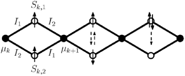
Fig. 1.: Schematic diagram of a fragment in an asymmetric diamond Ising–Hubbard chain. Solid and hollow circles denote nodes and interstitial positions, respectively. For the $k$-th primitive cell, the nodal spins, $\mu_{k}$, the $z$-components of total spins in the interstitial positions, $S_{k,i}$, and the parameters of the Ising interaction for bonds along the diamond sides, $I_{i}$, are indicated

The Hamiltonian $\mathcal{H}$ of the chain is written down as a sum of cell Hamiltonians $\mathcal{H}_{k}$,

$$\mathcal{H}=\!\!\sum\limits_{k=1}^{N}\mathcal{H}_{k},$$

$$\mathcal{H}_{k}{=}\!\!\sum\limits_{\sigma{\in}\{\uparrow,\downarrow\}}\!\!\!t\big{(}c_{k,1;\sigma}^{{\dagger}}c_{k,2;\sigma}+c_{k,2;\sigma}^{{\dagger}}c_{k,1;\sigma}\big{)}\!-$$

$$-\!\sum\limits_{i=1}^{2}Un_{k,i;\uparrow}n_{k,i;\downarrow}+$$

$${}+\mu_{k}(I_{1}S_{k,1}+I_{2}S_{k,2})+\mu_{k+1}(I_{2}S_{k,1}+I_{1}S_{k,2})-$$

$${}-h_{\text{e}}(S_{k,1}+S_{k,2})-\frac{1}{2}{h_{\text{i}}}(\mu_{k}+\mu_{k+1}),$$ (1)

where $N$ is the number of primitive cells in the chain; $c_{k,i;\sigma}^{{\dagger}}$ and $c_{k,i;\sigma}$ are the operators of creation and annihilation, respectively, of an electron with the spin $\sigma\in\{\uparrow,\downarrow\}$ at the interstitial position $(k,i)$; $n_{k,i;\sigma}=c_{k,i;\sigma}^{{\dagger}}c_{k,i;\sigma}$ is the operator of electron number; $\mu_{k}$ is the $z$-component of the spin-1/2 operator; $S_{k,i}=(n_{k,i;\uparrow}-n_{k,i;\downarrow})/2$ is the $z$-component of the operator of total electron spin at the interstitial position $(k,i)$; $t$ is the transfer integral; $U$ is the magnitude of the on-site electron-electron attraction ($U\geq 0$); $I_{1}$ and $I_{2}$ are the parameters of the Ising interaction for the bonds along the diamond sides (this interaction being identical only for collinear bonds) (Fig. 1); and $h_{\text{e}}$ and $h_{\text{i}}$ are magnetic fields that act on electron spins and Ising spins, respectively. It should be noted that Hamiltonian (1) also corresponds to a simple Ising–Hubbard chain (the nodes and interstitial positions are aligned), in which the Ising spin $\mu_{k}$ is coupled with the first, $I_{1}$, and second, $I_{2}$, neighbors.

The replacement of the on-site electron-electron attraction by a repulsion in Hamiltonian (1) transforms it into the chain Hamiltonian from work [24], which was solved exactly by applying the decoration-iteration transformation. Therefore, the exact solution for our chain can be obtained by replacing the on-site electron-electron repulsion by the attraction ($U\rightarrow-U$) in all results of work [24]. The spectrum of the Hamiltonian $\mathcal{H}_{k}$ obtained in such a way looks like

$$\mathcal{E}_{1}(\mu_{k},\mu_{k+1})=\frac{I_{1}+I_{2}}{2}(\mu_{k}+\mu_{k+1})\!-\!h_{\textrm{e}}-$$

$$-\frac{h_{\textrm{i}}}{2}(\mu_{k}\!+\!\mu_{k+1}),$$

$$\mathcal{E}_{2}(\mu_{k},\mu_{k+1})=-\frac{I_{1}+I_{2}}{2}(\mu_{k}+\mu_{k+1})\!+\!h_{\textrm{e}}-$$

$$-\frac{h_{\textrm{i}}}{2}(\mu_{k}\!+\!\mu_{k+1}),$$

$$\mathcal{E}_{3}(\mu_{k},\mu_{k+1})=\Lambda_{1}|\mu_{k}-\mu_{k+1}|-\frac{h_{\textrm{i}}}{2}(\mu_{k}+\mu_{k+1}),$$

$$\mathcal{E}_{4}(\mu_{k},\mu_{k+1})=\frac{1}{2}\left(\!\sqrt{U^{2}+16t^{2}}-U\!\right)|\mu_{k}+\mu_{k+1}|+$$

$${}+\Lambda_{2}|\mu_{k}-\mu_{k+1}|-\frac{h_{\textrm{i}}}{2}(\mu_{k}+\mu_{k+1}),$$

$$\mathcal{E}_{5}(\mu_{k},\mu_{k+1})=-\frac{1}{2}\left(\!\sqrt{U^{2}+16t^{2}}+U\!\right)|\mu_{k}+\mu_{k+1}|+$$

$${}+\Lambda_{3}|\mu_{k}-\mu_{k+1}|-\frac{h_{\textrm{i}}}{2}(\mu_{k}+\mu_{k+1}),$$

$$\mathcal{E}_{6}(\mu_{k},\mu_{k+1})=-U-\frac{h_{\textrm{i}}}{2}(\mu_{k}+\mu_{k+1}),$$ (2)

where $\Lambda_{3}<\Lambda_{1}<\Lambda_{2}$ are the eigenvalues of the matrix

$$\mathcal{L}=\left(\!\!\begin{array}[c]{ccc}0&\frac{I_{1}-I_{2}}{2}&0\\ \frac{I_{1}-I_{2}}{2}&0&2t\\ 0&2t&-U\end{array}\!\!\right)\!.$$

From this spectrum, the ground state and the parameters of a decoration-iteration transformation can be determined [24].

3 Numerical Results and Their Discussion

Consider the properties of our chain in the case of the antiferromagnetic Ising interaction ($I_{i}>0$), when there exists a geometrical frustration in it. The magnetic fields are put to be identical, $h=h_{\text{i}}=h_{\text{e}}$. Without any loss of generality, we adopt that $I_{1}\geq I_{2}$ and introduce the parameter $\Delta I=I_{1}-I_{2}$, similar to what was done in work [16]. Let us pass to the dimensionless parameters,

$$\tilde{t}=\frac{t}{I_{1}},\quad\tilde{U}=\frac{U}{I_{1}},\quad\Delta\tilde{I}=\frac{\Delta I}{I_{1}},\quad\tilde{h}=\frac{h}{I_{1}}.$$

It will be recalled that the parameter $\Delta\tilde{I}\in[0,1]$ characterizes the degree of asymmetry for the Ising interaction along the diamond sides [24].

Consider firstly the properties of the system in the ground state. The latter corresponds to the minimum energy in spectrum (2) for all possible configurations $\mu_{k}$ and $\mu_{k+1}$. Depending on the parameters $\tilde{t}$, $\tilde{U}$, $\Delta\tilde{I}$, and $\tilde{h}$, the system concerned can be in four ground states – similarly to what take place at $\tilde{U}\leqslant 0$ [16,​ 24] – namely, the saturated paramagnetic (SPA), ferrimagnetic (FRI), nonsaturated paramagnetic (UPA), and nodal antiferromagnetic (NAF) states. The energies of those states per cell are [24]

$$\tilde{\mathcal{E}}_{\text{SPA}}=1-\frac{\Delta\tilde{I}}{2}-\frac{3\tilde{h}}{2},\quad\tilde{\mathcal{E}}_{\text{FRI}}=-1+\frac{\Delta\tilde{I}}{2}-\frac{\tilde{h}}{2},$$

$$\tilde{\mathcal{E}}_{\text{UPA}}=-\frac{1}{2}\left(\tilde{U}+\sqrt{\tilde{U}^{2}+16\tilde{t}^{2}}\right)-\frac{\tilde{h}}{2},\quad\tilde{\mathcal{E}}_{\text{NAF}}=\tilde{\Lambda}_{3},$$

Fig. 2.: Phase diagram $(\Delta\tilde{I},\tilde{h})$ for the ground state. Transition lines for two sets of $\tilde{t}$- and $\tilde{U}$-values are shown. The results obtained for $\tilde{U}=0$ coincide with those of work [16]

where $\tilde{\Lambda}_{i}$ are the eigenvalues of the matrix $\tilde{\mathcal{L}}=\mathcal{L}/{I_{1}}$. The wave functions of those states are [24]

$$|\text{SPA}\rangle=\prod\limits_{k=1}^{N}{|+\rangle}_{k}\leavevmode\nobreak\ {|\uparrow,\uparrow\rangle}_{k,1;k,2},$$

$$|\text{FRI}\rangle=\prod\limits_{k=1}^{N}{|-\rangle}_{k}\leavevmode\nobreak\ {|\uparrow,\uparrow\rangle}_{k,1;k,2},$$

$$|\text{UPA}\rangle=\prod\limits_{k=1}^{N}{|+\rangle}_{k}\leavevmode\nobreak\ \left[\Psi_{5}^{++}\right]_{k,1;k,2},$$

$$|\text{NAF}\rangle=\left\{\!\!\begin{array}[c]{l}\prod\limits_{k=1}^{N}\left|(-)^{k}\right\rangle_{k}\leavevmode\nobreak\ \left[\Psi_{5}^{(-)^{k}(-)^{k+1}}\right]_{k,1;k,2}\\[11.38109pt] \prod\limits_{k=1}^{N}\left|(-)^{k+1}\right\rangle_{k}\leavevmode\nobreak\ \left[\Psi_{5}^{(-)^{k+1}(-)^{k+2}}\right]_{k,1;k,2}\end{array}\right.\!\!,$$

where $|+\rangle_{k}=|\uparrow\rangle_{k},$ and $|-\rangle_{k}=|\downarrow\rangle_{k}$ describe the state of spin $\mu_{k}$, $|\uparrow,\uparrow\rangle_{k,1;k,2}=c_{k,1;\uparrow}^{{\dagger}}c_{k,2;\uparrow}^{{\dagger}}|0\rangle$, and the notation $(-)^{n}$ means the sign of $(-1)^{n}$. The other notations are

$$\Psi_{5}^{++}\!=\!A_{5}^{++}\big{(}|\uparrow,\downarrow\rangle+|\downarrow,\uparrow\rangle\big{)}+B_{5}^{++}\big{(}|\uparrow\downarrow,0\rangle+|0,\uparrow\downarrow\rangle\big{)},$$

$$\Psi_{5}^{\pm\mp}\!=\!A_{5}^{\pm\mp}|\uparrow,\downarrow\rangle+A_{5}^{\mp\pm}|\downarrow,\uparrow\rangle+B_{5}^{+-}\big{(}|\uparrow\downarrow,0\rangle+|0,\uparrow\downarrow\rangle\big{)},$$

where

$$|\uparrow,\downarrow\rangle=c_{k,1;\uparrow}^{{\dagger}}c_{k,2;\downarrow}^{{\dagger}}|0\rangle,\leavevmode\nobreak\ \leavevmode\nobreak\ \leavevmode\nobreak\ \leavevmode\nobreak\ |\downarrow,\uparrow\rangle=-c_{k,1;\downarrow}^{{\dagger}}c_{k,2;\uparrow}^{{\dagger}}|0\rangle,$$

$$|\uparrow\downarrow,0\rangle=c_{k,1;\uparrow}^{{\dagger}}c_{k,1;\downarrow}^{{\dagger}}|0\rangle,\leavevmode\nobreak\ \leavevmode\nobreak\ \leavevmode\nobreak\ |0,\uparrow\downarrow\rangle=c_{k,2;\uparrow}^{{\dagger}}c_{k,2;\downarrow}^{{\dagger}}|0\rangle,$$

and the quantities $A_{5}^{++}$, $B_{5}^{++}$, $A_{5}^{+-}$, $A_{5}^{-+}$, and $B_{5}^{+-}$ are obtained from the corresponding coefficients in work [24] by replacing $\tilde{U}\rightarrow-\tilde{U}$.

Fig. 3.: Topological diagram $(\tilde{t},\tilde{U})$ for the phase diagram of the ground state, $(\Delta\tilde{I},\tilde{h})$, with “equitopological” lines. Bold lines separate the ranges of three typical topologies designated by the corresponding figures

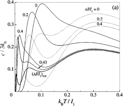
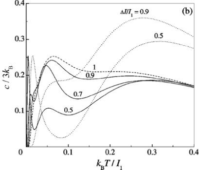
Fig. 4.: Temperature dependences of the zero-field heat capacity at various $\Delta\tilde{I}$: (a) $\Delta\tilde{I}\leq\Delta\tilde{I}_{\text{F.N}}$ and (b) $\Delta\tilde{I}>\Delta\tilde{I}_{\text{F.N}}$. Solid and dashed curves correspond to the results obtained for $\tilde{t}=0.15$ and $\tilde{U}=0.63$. Dotted curves show the results obtained for $\tilde{t}=0.375$ and $\tilde{U}=0$, which were exhibited in work [16] except for the curve for $\Delta\tilde{I}=0.4$

Let us consider the phase diagram for the ground state, $(\Delta\tilde{I},\tilde{h})$, which depends on the parameters $\tilde{t}$ and $\tilde{U}$. One of the possible phase diagrams $(\Delta\tilde{I},\tilde{h})$ is depicted in Fig. 2. The FRI and UPA states in it are separated by the transition line $\Delta\tilde{I}_{\text{F$|$U}}=\tilde{\mathcal{T}}(\tilde{t},\tilde{U})$, where $\tilde{\mathcal{T}}(\tilde{t},\tilde{U})=2-\tilde{U}-\sqrt{{\tilde{U}}^{2}+16\tilde{t}^{2}}$. The critical point between the FRI and NAF states in the zero field, $\Delta\tilde{I}_{\text{F.N}}$, is determined from the equation $\Delta\tilde{I}_{\text{F.N}}=2+2\tilde{\mathcal{E}}_{\text{NAF}}$.

The topology of the phase diagram $(\Delta\tilde{I},\tilde{h})$ for the ground state belongs to one of three types, depending on the parameters $\tilde{t}$ and $\tilde{U}$. The topology type is determined by the parameter $\tilde{\mathcal{T}}(\tilde{t},\tilde{U})$. The first type of the phase diagram topology is realized at $1\leq\tilde{\mathcal{T}}$. In this case, it looks as a part of Fig. 2 within the interval $[0,\Delta\tilde{I}_{\text{F$|$U}}]$ [16,​ 24]. The second topology type is realized at $0<\tilde{\mathcal{T}}<1$ (see Fig. 2). The third topology type is realized at $\tilde{\mathcal{T}}\leq 0$. In this case, the phase diagram $(\Delta\tilde{I},\tilde{h})$ looks like a part of Fig. 2 within the interval $[\Delta\tilde{I}_{\text{F$|$U}},1]$, but now the line of the NAF $\leftrightarrow$ UPA transition always begins at the point (0,0) [16,​ 24].

It is convenient to represent the dependence of the $(\Delta\tilde{I},\tilde{h})$ phase diagram topology on the parameters $\tilde{t}$ and $\tilde{U}$ in the form of a topological diagram ($\tilde{t},\tilde{U}$), which is shown in Fig. 3. “Equitopological” lines in this diagram are described by the equation $\tilde{\mathcal{T}}(\tilde{t},\tilde{U})=$const. The changes of $\tilde{U}$ and $\tilde{t}$ along the “equitopological” line are reflected in the phase diagram $(\Delta\tilde{I},\tilde{h})$ as a displacement of only those lines that bound the range of the ground NAF state, which is demonstrated in Fig. 2. In particular, as the parameter $\tilde{U}$ grows, the range of the ground NAF state in it decreases.

Now consider the influence of the on-site electron-electron attraction on the magnetization, magnetic susceptibility, and heat capacity in the regime $\tilde{\mathcal{T}}(\tilde{t},\tilde{U})=\mathrm{const}$, i.e. along an “equitopological” line. Numerical calculations of those characteristics were carried out for a number of points $(\tilde{t},\tilde{U})$ along the “equitopological” line that belongs to region 2 in Fig. 3 and passes through the points $(0.375,0)$ and $(0.15,0.63)$, for which the phase diagram $(\Delta\tilde{I},\tilde{h})$ of the ground state is exhibited in Fig. 2.

A comparison of the results obtained for the magnetization and the magnetic susceptibility at various points on the “equitopological” line shows that the field and temperature curves of magnetization and the temperature curve of magnetic susceptibility in the zero field shift at strengthening the attraction, similarly to what takes place at weakening the on-site electron-electron repulsion [24]. In particular, if the attraction becomes stronger, the temperature curves of total and electron magnetizations shift downward, and the temperature curve of magnetization for Ising spins shifts upward.

The modification of the temperature dependence of the zero-field heat capacity under the influence of the attraction is shown in Fig. 4. In the absence of attraction ($\tilde{U}=0$), the temperature curve of the heat capacity has the main and low-temperature maxima in a wide range of $\Delta\tilde{I}$ [16]. In a certain vicinity of the critical point $\Delta\tilde{I}_{\text{F.N}}$, it has another low-temperature maximum, which is the closest to the zero temperature [24]. While the attraction grows to a definite value of about 0.42, the main maximum shifts toward lower temperatures. However, if the attraction grows further, the maximum shifts back toward higher temperatures. As a result, the main maximum of the curves that correspond to small $\Delta\tilde{I}$ can merge with the low-temperature maximum (Fig. 4). Moreover, starting from $\tilde{U}\simeq 0.5$, there emerges an additional maximum in the temperature dependence of the heat capacity, which is located between the low-temperature and main maxima (Fig. 4). At first, this additional maximum exists within a small interval for $\Delta\tilde{I}$ in the range of the ground NAF state. As the attraction becomes stronger, this interval broadens and surrounds the critical point $\Delta\tilde{I}_{\text{F.N}}$ (Fig. 4). The modification in the temperature dependence of the zero-field heat capacity induced by the attraction growth is associated with changes in spectrum (2) of the cell Hamiltonian $\mathcal{H}_{k}$. Namely, as the parameter $\tilde{U}$ increases, the energies $\mathcal{E}_{6}$, $\mathcal{E}_{4}({\Lambda}_{2})$, and $\mathcal{E}_{3}({\Lambda}_{1})$ in this spectrum decrease.

It is also worth noting that the temperature curve of the heat capacity for $\tilde{U}=0.63$ has an additional low-temperature maximum in a very close–much narrower than at $\tilde{U}=0$–vicinity to the critical point $\Delta\tilde{I}_{\text{F.N}}$. This maximum, which is the nearest to the zero temperature, was described in detail in work [24].

4 Conclusions

In this work, the properties of an asymmetric diamond Ising–Hubbard chain with the on-site electron-electron attraction are studied in the ground state at finite temperatures. It is an example of the exact solution obtained with the use of the decoration-iteration transformation. In the case of the antiferromagnetic Ising interaction, when there is a geometrical frustration in the chain, the influence of the on-site electron-electron attraction on the ground state, the field and temperature dependences of the magnetization, and the temperature dependences of the zero-field magnetic susceptibility and the heat capacity are studied.

The phase diagram for the ground state is plotted in the plane $(\Delta\tilde{I},\tilde{h})$. A modifications of this phase diagram induced by the transfer integral and the on-site attraction is represented in the form of a topological diagram $(\tilde{t},\tilde{U})$. It is shown that strengthening the attraction along the “equitopological” line $\tilde{\mathcal{T}}(\tilde{t},\tilde{U})=\mathrm{const}$ is reflected in the phase diagram ($\Delta\tilde{I},\tilde{h}$) as a displacement of the ground NAF state boundaries so that the corresponding confined area becomes smaller.

As the on-site electron-electron attraction becomes stronger along the “equitopological” line, the temperature curves of the magnetization, at various fields, and the zero-field magnetic susceptibility shift, as it was in the case of weakening the on-site electron-electron repulsion [24]. The temperature dependence of the zero-field heat capacity in a certain range $(\tilde{t},\tilde{U},\Delta\tilde{I})$ has an additional maximum between the main and low-temperature maxima.

The results of this work also correspond to a simple Ising–Hubbard chain, in which the nodes and the interstitial positions are aligned, and the nodal Ising spin is coupled with those of the first and second neighbors.

Б.М. Лiсний
АСИМЕТРИЧНИЙ РОМБIЧНИЙ ЛАНЦЮЖОК
IЗIНГА–ГАББАРДА З ПРИТЯГАННЯМ
Р е з ю м е
Розглянуто основний стан i термодинамiчнi властивостi асиметричного ромбiчного ланцюжка Iзiнга–Габбарда з одноцентровим електрон-електронним притяганням, який є точно розв’язуваним за допомогою декорацiйно-iтерацiйного перетворення. У випадку антиферомагнiтної взаємодiї Iзiнга вивчено вплив цього притягання на основний стан i температурну залежнiсть намагнiченостi, магнiтної сприйнятливостi та теплоємностi.

References

- [1] I. Syozi, Prog. Theor. Phys. 6, 341 (1951).
- [2] M. Fisher, Phys. Rev. 113, 969 (1959).
- [3] J. Strečka, Phys. Lett. A 374, 3718 (2010).
- [4] O. Rojas and S.M. de Souza, J. Phys. A 44, 245001 (2011).
- [5] H. Kikuchi, Y. Fujii, M. Chiba, S. Mitsudo, T. Idehara, T. Tonegawa, K. Okamoto, T. Sakai, T. Kuwai, and H. Ohta, Phys. Rev. Lett. 94, 227201 (2005).
- [6] H. Kikuchi, Y. Fujii, M. Chiba, S. Mitsudo, T. Idehara, T. Tonegawa, K. Okamoto, T. Sakai, T. Kuwai, K. Kindo, A. Matsuo, W. Higemoto, K. Nishiyama, M. Horvatić and C. Bertheir, Prog. Theor. Phys. Suppl. 159, 1 (2005).
- [7] J. Strečka, M. Jaščur, M. Hagiwara, K. Minami, Y. Narumi, and K. Kindo, Phys. Rev. B 72, 024459 (2005).
- [8] L. Čanová, J. Strečka, and M. Jaščur, J. Phys. Condens. Matter 18, 4967 (2006).
- [9] L. Čanová, J. Strečka, and T. Lučivjanský, Condens. Matter Phys. 12, 353 (2009).
- [10] B.M. Lisnyi, Ukr. J. Phys. 56, 1237 (2011).
- [11] W. Van den Heuvel and L.F. Chibotaru, Phys. Rev. B 82, 174436 (2010).
- [12] V.R. Ohanyan and N.S. Ananikian, Phys. Lett. A 307, 76 (2003).
- [13] J. Strečka and M. Jaščur, J. Phys. Condens. Matter 15, 4519 (2003).
- [14] J.S. Valverde, O. Rojas, and S.M. de Souza, Physica A 387, 1947 (2008).
- [15] J.S. Valverde, O. Rojas, and S.M. de Souza, J. Phys. Condens. Matter 20, 345208 (2008).
- [16] M.S.S. Pereira, F.A.B.F. de Moura, and M.L. Lyra, Phys. Rev. B 77, 024402 (2008).
- [17] M.S.S. Pereira, F.A.B.F. de Moura, and M.L. Lyra, Phys. Rev. B 79, 054427 (2009).
- [18] V. Ohanyan, Condens. Matter Phys. 12, 343 (2009).
- [19] D. Antonosyan, S. Bellucci, and V. Ohanyan, Phys. Rev. B 79, 014432 (2009).
- [20] O. Rojas and S.M. de Souza, Phys. Lett. A 375, 1295 (2011).
- [21] O. Rojas, S.M. de Souza, V. Ohanyan, and M. Khurshudyan, Phys. Rev. B 83, 094430 (2011).
- [22] J. Strečka, A. Tanaka, L. Čanová, and T. Verkholyak, Phys. Rev. B 80, 174410 (2009).
- [23] L. Gálisová, J. Strečka, A. Tanaka, and T. Verkholyak, J. Phys. Condens. Matter 23, 175602 (2011).
- [24] B.M. Lisnyi, Low Temp. Phys. 37, 296 (2011).
- [25] J.E. Hirsch, Phys. Rev. B 31, 6022 (1985).
- [26] M.E. Zhuravlev, V.A. Ivanov, and V.V. Achkasov, Pis’ma Zh. Eksp. Teor. Fiz. 63, 83 (1996).
-
[27]
Q. Wang and H. Zheng, Phys. Lett. A 314, 304
(2003).
Received 29.05.12.
Translated from Ukrainian by O.I. Voitenko