Center Vortices and Chiral Symmetry Breaking in $SU(2)$ Lattice Gauge Theory

Abstract

We investigate the chiral properties of near-zero modes for thick classical center vortices in $SU(2)$ lattice gauge theory as examples of the phenomena which may arise in a vortex vacuum. In particular we analyze the creation of near-zero modes from would-be zero modes of various topological charge contributions from center vortices. We show that classical colorful spherical vortex and instanton ensembles have almost identical Dirac spectra and the low-lying eigenmodes from spherical vortices show all characteristic properties for chiral symmetry breaking. We further show that also vortex intersections are able to give rise to a finite density of near-zero modes, leading to chiral symmetry breaking via the Banks-Casher formula. We discuss the mechanism by which center vortex fluxes contribute to chiral symmetry breaking.

I Introduction

Quantum chromodynamics (QCD) at low energies is dominated by the nonperturbative phenomena of quark confinement and spontaneous chiral symmetry breaking ($\chi$SB). Presently, a rigorous treatment of them is only possible in the lattice regularization. Many of the important features of non-Abelian gauge theories are already present in SU(2), which simplifies theoretical and numerical calculations.

The nonperturbative vacuum can be characterized by various kinds of topological gauge field excitations. A well established theory of $\chi$SB relies on instantons Belavin:1975fg ; Actor:1979in ; 'tHooft:1976fv ; Bernard:1979qt , which are localized in space-time and carry a topological charge of modulus $1$. According to the Atiyah-Singer index theorem Atiyah:1971rm ; Schwarz:1977az ; Brown:1977bj ; Narayanan:1994gw , a zero mode of the Dirac operator arises, which is concentrated at the instanton core. In the instanton liquid model Ilgenfritz:1980vj ; Diakonov:1984vw ; Diakonov:1986tv overlapping would-be zero modes split into low-lying nonzero modes which create the chiral condensate.

Center vortices 'tHooft:1977hy ; Vinciarelli:1978kp ; Yoneya:1978dt ; Cornwall:1979hz ; Mack:1978rq ; Nielsen:1979xu , on the other hand, are promising candidates for explaining confinement. They form closed magnetic flux tubes, whose flux is quantized, taking only values in the center of the gauge group. These properties are the key ingredients in the vortex model of confinement, which is theoretically appealing and was also confirmed by a multitude of numerical calculations, both in lattice Yang-Mills theory and within a corresponding infrared effective model, see e.g. DelDebbio:1996mh ; Langfeld:1997jx ; DelDebbio:1997ke ; Kovacs:1998xm ; Engelhardt:1999wr ; Bertle:2002mm ; Engelhardt:2003wm . Lattice simulations indicate that vortices may be responsible for topological charge and $\chi$SB as well deForcrand:1999ms ; Alexandrou:1999vx ; Reinhardt:2000ck2 ; Engelhardt:2002qs ; Bornyakov:2007fz ; Hollwieser:2008tq , and thus unify all nonperturbative phenomena in a common framework. A similar picture to the instanton liquid model exists insofar as lumps of topological charge arise at the intersection and writhing points of vortices. The colorful, spherical SU(2) vortex as introduced in previous articles of our group Jordan:2007ff ; Hollwieser:2010mj ; Hollwieser:2012kb ; Schweigler:2012ae , may act as a prototype for this picture, as it contributes to the topological charge by its color structure, attracting a zero mode like an instanton.

In this article we want to show how the interplay of various topological structures from center vortices (and instantons) leads to near-zero modes, which by the Banks-Casher relation Banks:1979yr are responsible for a finite chiral condensate. Using the overlap and asqtad staggered Dirac operator, we compute a varying number of the lowest-lying Dirac eigenfunctions, including the zero modes. By visualizing the probability density, we compare the distribution of the eigenmode density with the position of the vortices and the topological charge created by intersection points and color structures. These results manifest the importance of center vortices also for chiral symmetry breaking.

II Topological charge from center vortices

From the definition

$$Q\propto\epsilon_{\mu\nu\alpha\beta}F_{\mu\nu}F_{\alpha\beta}\,,$$ (1)

it is clear that topological charge contributions arise where two perpendicular nontrivial plaquettes meet. On a center vortex, the vortex sheet is locally orthogonal to the nontrivial plaquettes. Hence, topological charge emerges at so-called singular points of center vortices, where the set of tangent vectors to the vortex surface spans all four space-time directions Reinhardt:2001kf . There are two possibilities where this can occur:

• intersection points of two different surface patches: $Q=\pm 1/2$   ,

• writhing points of a single surface patch: $|Q|<1/2$   .

In lattice language, intersection points have four plaquettes attached to them extending in two particular space time directions (e.g. $xy$), and another four plaquettes extending in the two orthogonal directions (e.g. $zt$). By contrast, at a writhing point one can start at any attached plaquette and pass around over all others along a continuous path since they are connected by common links.

In SU(2), a Wilson loop cannot distinguish between center fluxes of opposite sign, since $\exp(i\pi)=\exp(-i\pi)=-1$. However, the sign of the topological charge is sensitive to the direction of the flux. To preserve this information for thin vortices, one can assign an orientation to the vortex patches. Note that this quantity is not directly linked to the geometry of the vortex. A non-orientable vortex need not be non-orientable as a surface Bertle:1999tw .

Vortices always have closed surfaces. Furthermore, lattice studies show that the major fraction of vortex patches belongs to a single large vortex winding through the whole lattice. Intersections between different vortices are therefore only of minor importance. But for a closed oriented surface the total charge is zero. Charged vortices must therefore be globally non-oriented and consist of differently oriented patches, which are separated by monopole worldlines. The colorful spherical vortex is a classical representation of such a vortex configuration, contributing to topological charge only through its color structure. It will be discussed shortly in Sec. II.2, but first let us explain the relation between vortices and magnetic monopoles, thereby making precise the definition of the orientation of a vortex.

On the lattice, monopoles are located by so-called Abelian projection. First, one fixes the links up to a residual $U(1)$-symmetry, which corresponds to an Abelian gauge theory. For example, we can use the maximal Abelian gauge Greensite:2003bk to rotate the color vector of the links as much as possible in, say, the $\sigma_{3}$-direction by maximizing

$$R=\sum_{x,\mu}\mathrm{tr}[U_{\mu}(x)\sigma_{3}U_{\mu}^{\dagger}(x)\sigma_{3}]\,.$$ (2)

Afterwards, the link variables are replaced by their diagonal part

$$U_{\mu}(x)=a_{0}\mathbbm{1}+i\vec{a}\cdot\vec{\sigma}\rightarrow u_{\mu}(x)=\frac{1}{\sqrt{a_{0}^{2}+a_{3}^{2}}}[a_{0}\mathbbm{1}+ia_{3}\sigma_{3}]=\begin{pmatrix}\exp\{i\theta_{\mu}(x)\}&0\\ 0&\exp\{-i\theta_{\mu}(x)\}\end{pmatrix}\,.$$ (3)

Consider a 3-dimensional cube on the lattice. Normally, the total magnetic flux out of the cube vanishes due to $\mathrm{div}\,\vec{B}=0$. If the cube contains a monopole, there would be a nonzero net flux of the (nonphysical) Dirac string, which compensates the physical monopole flux. The magnetic charge inside the cube is defined by Chernodub:2001ht

$$m=\frac{1}{2\pi}\sum_{p}\bar{\theta}_{p}\,.$$ (4)

$\theta_{p}$ is the sum of the angles $\theta_{\mu}$ around one plaquette $p$; $\sum_{p}\theta_{p}$ is always zero as a consequence of the Bianchi identity. $\bar{\theta}_{p}$ is $\theta_{p}+2\pi k$ with $k$ such that $\bar{\theta}_{p}$ falls into the range $[-\pi,\pi]$. If the absolute value of all plaquette angles is smaller than $\pi$, $\bar{\theta}_{p}=\theta_{p}$ and $m=0$, as usual. Plaquettes which are greater than $\pi$ are pierced by the Dirac string, at the end of which a monopole is located. $\bar{\theta}_{p}$ discards the flux caused by the Dirac string and a value $m\neq 0$ results.

Now let us return to center vortices. Traversing a thick vortex sheet, the link variables change gradually, building up to a center element. Pictured in group space of $SU(2)\simeq S^{3}$, we travel along a path from unity to the antipode $-\mathbbm{1}$. After Abelian projection, only one possible direction for the path remains and this path will go either in $+\sigma_{3}$ or in $-\sigma_{3}$ direction. We can use this sign to allocate an orientation to every patch of the vortex surface. The sign also corresponds to the direction of the center flux bundled within the vortex, which is quantized in units $\pm\pi$. Where regions of opposite orientation touch, the flux jumps by $2\pi$, indicating the presence of a sink or source, i.e., a magnetic monopole carrying a quantized magnetic charge. To summarize, a center vortex can be imagined as a chain of magnetic monopoles, whose flux is bundled within the vortex surface. The monopole worldlines divide the vortex sheet into patches of different orientations.

II.1 Plane vortices

We define plane vortices parallel to two of the coordinate axes by links varying in a $U(1)$ subgroup of $SU(2)$. This $U(1)$ subgroup is generated by one of the Pauli matrices $\sigma_{i}$, i.e., $U_{\mu}=\exp(\mathrm{i}\phi\sigma_{i})$. The direction of the flux and the orientation of the vortices are determined by the gradient of the angle $\phi$, which we choose as a piece wise linear function of a coordinate perpendicular to the vortex. The explicit functions for $\phi$ are given in Eq. (2.1) of Hollwieser:2011uj (see also Fig.1 therein). Upon traversing a vortex sheet, the angle $\phi$ increases or decreases by $\pi$ within a finite thickness of the vortex. Since we use periodic (untwisted) boundary conditions for the links, vortices occur in pairs of parallel sheets, each of which is closed by virtue of the lattice periodicity. We call vortex pairs with the same vortex orientation parallel vortices and vortex pairs of opposite flux direction anti-parallel. Of course, there are always two coordinates perpendicular to a vortex surface, and vortices are always thin in one of these directions. Their cross-sections thus strictly speaking do not correspond to thickened tubes of magnetic flux, but rather thin strips. If the thick, planar vortices intersect orthogonally, each intersection carries a topological charge with modulus $|Q|=1/2$, whose sign depends on the relative orientation of the vortex fluxes Engelhardt:1999xw , see Fig. 1. Fig. 1b indicates the position of the vortices after center projection, leading to (thin) P-vortices at half the thickness DelDebbio:1996mh .

Parallel Vortices	Geometry	Anti-parallel Vortices
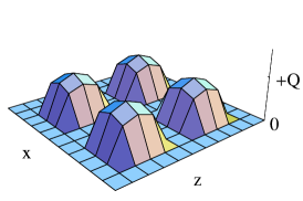
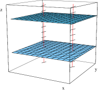
a)	b)	c)

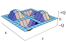
Figure 1: A single time slice of a $12^{4}$-lattice with intersecting vortices (center). The horizontal planes are the $xy$-vortices, which exist only at this time. The vertical lines are the $zt$-vortices, which continue over the whole time axis. The vortices intersect in four points, giving topological charge $Q=2$ for parallel vortices (lhs) or $Q=0$ for anti-parallel vortices (rhs).

II.2 The Colorful Spherical Vortex

The non-orientable spherical vortex of radius $R$ and thickness $\Delta$ was introduced in Jordan:2007ff and analyzed in more detail in Hollwieser:2010mj and Schweigler:2012ae . It is constructed with the following $SU(2)$ links:

$$U_{\mu}(x_{\nu})=\begin{cases}\exp\left(\mathrm{i}\alpha(|\vec{r}-\vec{r}_{0}|)\vec{n}\cdot\vec{\sigma}\right)&t=t_{i},\mu=4\\ \mathbbm{1}&\mathrm{elsewhere}\end{cases}\quad\mbox{with}\quad\vec{n}(\vec{r},t)=\frac{\vec{r}-\vec{r}_{0}}{|\vec{r}-\vec{r}_{0}|}\,,$$ (5)

where $\vec{r}$ is the spatial part of $x_{\nu}$ and the profile function $\alpha$ is either one of $\alpha_{+},\alpha_{-}$, which are defined by

$$\alpha_{-}(r)=\begin{cases}\pi\\ \frac{\pi}{2}\left(1-\frac{r-R}{\frac{\Delta}{2}}\right)\\ 0\end{cases}\ldots\;\alpha_{+}(r)=\begin{cases}\pi&r<R-\frac{\Delta}{2}\\ \frac{\pi}{2}\left(3+\frac{r-R}{\frac{\Delta}{2}}\right)&R-\frac{\Delta}{2}<r<R+\frac{\Delta}{2}\\ 2\pi&R+\frac{\Delta}{2}<r\end{cases}\,.$$ (6)

This means that all links are equal to $\mathbbm{1}$ except for the $t$-links in a single time slice at fixed $t=t_{i}$. The phase changes from $\pi$ to $0$ within a thickness $\Delta$ for $\alpha_{-}(r)$ (or from $\pi$ to $2\pi$ for $\alpha_{+}(r)$). The graph of $\alpha_{-}(r)$ is plotted in Fig. 2 in Jordan:2007ff , giving a hedgehog-like configuration, since the color vector $\vec{n}$ points in the “radial” direction $\vec{r}/r$ at the vortex radius $R$, see Fig. 2a. The check that this configuration is a vortex is done with maximal center gauge fixing and center projection and results in a P-vortex forming a lattice representation of a 3-sphere of radius $R$ at time slice $t_{i}$, see Fig. 2c. The color structure of the thick vortex leads to a monopole loop on a great circle of the P-vortex after fixing to maximal Abelian gauge and Abelian projection. The direction of the loop depends on the $U(1)$ subgroup chosen as Abelian degrees of freedom. For the subgroup defined by the Pauli matrices $\sigma_{1},\sigma_{2}$ or $\sigma_{3}$ the monopole loops are in the $yz$-, $zx$- and $xy$-plane, respectively. This is indicated schematically in Fig. 2b with three colors.

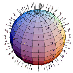
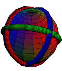
a) b) c)

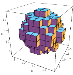
Figure 2: a) The color structure of the vortex surface from the hedgehog configuration leads to b) monopole lines after Abelian projection in the maximal Abelian gauge. c) Lattice representation of a 3-sphere for our spherical vortex after center projection in maximal center gauge.

The hedgehog-like structure is crucial for our analysis. The $t$-links of the spherical vortices fix the holonomy of the time-like loops, defining a map $U_{t}(\vec{x},t=t_{i})$ from the $xyz$-hyperplane at $t=t_{i}$ to $SU(2)$. Because of the periodic boundary conditions, the time slice has the topology of a 3-torus. But, actually, we can identify all points in the exterior of the 3 dimensional sphere since the links there are trivial. Thus the topology of the time slice is $\mathbbm{R}^{3}\cup\{\infty\}$ which is homeomorphic to $S^{3}$. A map $S^{3}\to SU(2)$ is characterized by a winding number

$$N=-\frac{1}{24\pi^{2}}\int d^{3}x\,\epsilon_{ijk}\,\mbox{Tr}[(U^{\dagger}\partial_{i}U)(U^{\dagger}\partial_{j}U)(U^{\dagger}\partial_{k}U)],$$

resulting in $N=-1$ for positive and $N=+1$ for negative spherical vortices. Obviously such windings, given by the holonomy of the time-like loops of the spherical vortex, influence the Atiyah-Singer index theorem Atiyah:1971rm ; Schwarz:1977az ; Brown:1977bj ; Narayanan:1994gw ; Nye:2000eg ; Poppitz:2008hr , giving a topological charge $Q=-1$ for positive and $Q=+1$ for negative spherical vortices (anti-vortices). Hence, spherical vortices attract Dirac zero modes similar to instantons. In Schweigler:2012ae we showed that the spherical vortex is in fact a vacuum-to-vacuum transition in the time direction which can even be regularized (smoothed out in the time direction) to give the correct topological charge also from gluonic definitions (see also Schweigler:2012 for more details).

III Dirac eigenmodes

According to the Banks-Casher analysis Banks:1979yr , chiral symmetry breaking ($\chi$SB) is necessarily associated with a finite density of near-zero eigenmodes of the chiral-invariant Dirac operator, resulting in a finite chiral condensate, the order parameter of chiral symmetry breaking. We compute the lowest-lying chiral eigenvectors $\chi_{R,L}$ and eigenvalues $|\lambda|\in[0,1]$ of the overlap Dirac operator

$$D_{ov}=\frac{1}{2}\left[1+\frac{D_{W}}{\sqrt{D_{W}^{\dagger}D_{W}}}\right]$$ (7)

with the kernel Wilson Dirac operator $D_{W}$ Edwards:1998yw . Henceforth we will simply write $\lambda$ instead of $|\lambda|$ and assume it to be the absolute value of the two complex conjugate eigenvalues of $D_{ov}$ if $\lambda\neq 0,1$. We will however distinguish between right- and left-handed zero modes of $D_{ov}$. When speaking of an eigenmode, we always mean both of the eigenvectors $\psi_{\pm}$ belonging to one value of $\lambda\neq 0$, which have the same scalar and chiral densities. For convenience, we will number the eigenfunctions in ascending order of the eigenvalues. #0+ denotes the right-handed zero mode, #0– the left-handed zero mode. #1 labels the lowest nonzero mode, #2 the second lowest etc. Their eigenvalues are referred to as $\lambda$#0+, $\lambda$#0–, $\lambda$#1, etc., and their densities as $\rho$#0+, etc. Finally, we will name near-zero modes which emerge from would-be zero modes also by #0 for good reasons, which will be discussed later.

The corresponding eigenvectors are given by

$$\psi_{\pm}=\frac{1}{\sqrt{2}}(\chi_{R}\pm i\chi_{L}).$$ (8)

They have scalar and chiral densities

$$\rho=\psi^{\dagger}_{\pm}\psi_{\pm}=\frac{1}{2}(\chi_{R}^{\dagger}\chi_{R}+\chi_{L}^{\dagger}\chi_{L})\,,$$ (9)

$$\rho_{+}=\psi^{\dagger}_{\pm}\frac{1}{2}(1+\gamma_{5})\psi_{\pm}=\frac{1}{2}(\chi_{R}^{\dagger}\chi_{R})\,,$$ (10)

$$\rho_{-}=\psi^{\dagger}_{\pm}\frac{1}{2}(1-\gamma_{5})\psi_{\pm}=\frac{1}{2}(\chi_{L}^{\dagger}\chi_{L})\,,$$ (11)

$$\rho_{5}=\psi^{\dagger}_{\pm}\gamma_{5}\psi_{\pm}=\frac{1}{2}(\chi_{R}^{\dagger}\chi_{R}-\chi_{L}^{\dagger}\chi_{L})=\rho_{+}-\rho_{-}\,.$$ (12)

The chiral density $\rho_{5}$ is important to assess the local chirality properties, in particular to test the notion that the near-zero modes arise from the splitting of exact zero modes localized at lumps of topological charge.

In a gauge field with topological charge $Q\neq 0$, $D_{ov}$ has $|Q|$ exact zero modes with chirality $-\mathrm{sign}Q$, and an equal number of eigenvectors of opposite chirality and eigenvalue 1 (doubler modes). This is required in order that $\mbox{Tr}\gamma_{5}=0$. The topological charge is

$$Q=\mbox{Tr}(\gamma_{5}D_{ov})=n_{-}-n_{+}=\text{ind}D_{ov}\,,$$ (13)

as for any Ginsparg-Wilson operator.

The plot titles of the density plots (see e.g. Fig. 3) give the $x$- and $y$-coordinates of the shown $zt$-slice, the chirality (i.e., ”chi=0” means we plot $\rho_{5}$, ”chi=1” would be $\rho_{+}$ and ”chi=-1” $\rho_{-}$), the numbers of plotted modes (”n=1-1” means we plot $\rho\#1$, ”n=1-2” would be $\rho\#1+\rho\#2$) and the maximal density in the plotted area (”max=…” - some maxima are cut off in order to resolve other substructures). For instanton and spherical vortex configurations we use $12^{3}\times 24$-lattices and always plot $xt$-slices at $y=z=6$ since they are symmetric in spatial directions around their centers at $x=y=z=6.5$. For plane vortex configurations we use $16^{4}$-lattices, the plotted slices vary.

III.1 Eigenvalue Spectrum of the free Dirac operator

In this section we will analytically calculate the eigenvalues of the massless free Dirac operator. These eigenvalues and their multiplicity will come handy later when we compare the eigenvalues for different gauge field configurations to the eigenvalues for the free case. The free continuum Dirac operator for massless fermions is given by $D=\gamma_{\mu}\partial_{\mu}$, where $\gamma_{\mu}$ are the Euclidean Dirac matrices. We want to solve the Dirac equation $D_{\alpha\beta}\ \psi_{\beta}(x)=\lambda\ \psi_{\alpha}(x)$. Using the well know ansatz of plane wave functions $\psi_{\alpha}(x)=u_{\alpha}\ \exp(ip_{\mu}x_{\mu})$, one gets the eigenvalues of the free continuum operator $\lambda=\pm i\sqrt{p_{\mu}p_{\mu}}$. Identifying the eigenvalue $\lambda$ with the fermion mass $M$ makes clear, that this is simply the relativistic energy momentum relation in Euclidean space given by $M^{2}=E^{2}+p^{2}$, where we have denoted $p_{4}^{2}$ by $E^{2}$ and $p_{i}p_{i}$ by $p^{2}$. Note that both the eigenvalue for the plus and the minus sign have a degeneracy of two, which gives in total four eigenvalues for the $4\times 4$ Dirac matrix ($4\times 4$ Dirac indices). Additional degeneracy comes from the color indices. The free Dirac operator is color blind. Therefore, the degeneracy of the different eigenvalues is multiplied by $n_{col}$, where $n_{col}$ is the range of the color indices. For the overlap Dirac operator the eigenvalues can also be calculated analytically for the free case using the lattice ansatz $\psi_{\alpha}(n)=u_{\alpha}\ \exp(i\ a\ p_{\mu}n_{\mu})$, with the lattice sites $n_{\mu}$ and yield the continuum solutions with corrections of orders of $a^{2}$:

$$D_{ov}(p_{\mu})=\frac{1}{2}\left[1+\frac{i\gamma_{\mu}\sin(p_{\mu})-M(p_{\mu})}{\sqrt{\sum_{\mu}\sin(p_{\mu})^{2}+M^{2}(p_{\mu})}}\right]$$ (14)

with $M(p_{\mu})=M-\sum_{\mu}\left(1-\cos(p_{\mu})\right)$. Here $a=1$ and $M=1$ in the free case. This gives ($H_{ov}=\gamma_{5}D_{ov}$):

$$H^{2}_{ov}(p_{\mu})=D_{ov}^{\dagger}D_{ov}=\frac{1}{2}\left[1-\frac{M(p_{\mu})}{\sqrt{\sum_{\mu}\sin(p_{\mu})^{2}+M^{2}(p_{\mu})}}\right]=\lambda^{2}$$ (15)

with expected multiplicities ($H^{2}_{ov}(p_{\mu})$ is a diagonal $4\times 4$ matrix). For $p_{\mu}<<1$ we get

$$\lambda^{2}=\frac{p_{\mu}p_{\mu}}{4M^{2}}(1+O(p_{\mu}p_{\mu}))\,.$$ (16)

With the normalization of Eq. (7), which leads to $\lambda^{2}\in[0,1]$, a wave function renormalization is needed to convert to the usual continuum normalization. This compensates the factor $\frac{1}{4M^{2}}$, see e.g. Eq. (6) in Edwards:1998wx , giving the usual free Dirac eigenvalues in the continuum limit. Note that the plane wave ansatz is periodic, not only in $x_{\mu}$ or lattice indices $n_{\mu}$, but also in $p_{\mu}$. This means, that $p_{\mu}$ and $p_{\mu}+\frac{2\pi z_{\mu}}{a}$ (with $z_{\mu}\in\mathbb{Z}$) correspond to the same eigenfunction. Therefore, in order to get the correct multiplicities for the eigenvalues, we have to restrict the range of $p_{\mu}$ to

$$-\frac{\pi}{a}<p_{\mu}\leq\frac{\pi}{a}\,.$$ (17)

For the usual periodic boundary conditions in the spatial directions and periodic or anti-periodic boundary conditions in the temporal direction, the allowed values for $p_{\mu}$ are

$$p_{i}=\frac{2n\pi}{aN_{sp}},\quad\quad p_{4}=\begin{cases}\frac{2n\pi}{aN_{t}}&\mbox{for periodic BC}\\ \frac{(2n+1)\pi}{aN_{t}}&\mbox{for anti-periodic BC}\end{cases},\quad\quad n\in\mathbb{Z}\,,$$

where $N_{sp}$ is the spatial and $N_{t}$ the temporal extent of the lattice. The total multiplicity of an eigenvalue $\lambda$ is given by

$$n_{mult}(\lambda)=2\ n_{col}\ n_{p}(\lambda),$$

where $n_{p}(\lambda)$ is the number of different $p_{\mu}$ corresponding to a particular $\lambda$. The factor two comes from the Dirac indices as discussed above. Let us now have a quick look at the multiplicity of the eigenvalues for one particular lattice size, i.e., $N_{sp}=12$ and $N_{t}=24$, which we will use later for our lattice configurations. We assume anti-periodic boundary conditions in the temporal direction, $a=1$ and a $SU(2)$ gauge field theory (i.e., $n_{col}=2$). The momentum vectors corresponding to the lowest eigenvalues are then given by $p_{i}=0$ and $p_{4}=\pm\pi/24$. Therefore, we have $n_{p}(\lambda\#1)=2$ for the lowest eigenvalues $\lambda\#1$. That means, we get a multiplicity $n_{mult}(\lambda\#1)=2\ n_{col}\ n_{p}(\lambda\#1)=8$. For the second lowest eigenvalues $\lambda\#2$ we have $p_{i}=0$ and $p_{4}=\pm 3\pi/24=\pm\pi/8$ and therefore another degeneracy of eight. Then we get $p_{i}=\pm\pi/6$ (with $i\in\{1,2,3\}$) and $p_{4}=\pm\pi/24$, i.e., $n_{p}(\lambda\#3)=12$. This gives a multiplicity $n_{mult}(\lambda\#3)=48$.

Fig. 3 shows the chiral density of free overlap eigenmodes obtained numerically using the MILC code. The modes are found with the Ritz functional algorithm Bunk:1994uv ; Kalkreuter:1995mm with random start and for degenerate eigenvalues the eigenmodes span a randomly oriented basis in the degenerate subspace. Therefore the numerical modes presented in Fig. 3 are linear combinations of plane waves with $\pm p_{\mu}$ and show plane wave oscillations of $2p_{\mu}$ in the chiral density. The first eight degenerate modes consist of plane waves with $p_{4}=\pm\pi/24$, hence there is one sine (cosine) oscillation in time direction, the next eight have $p_{4}=\pm 3\pi/24$, i.e., three oscillations in the time direction. The oscillations of $\chi_{R}$ and $\chi_{L}$ are separated by half an oscillation length, i.e., the maxima of $\rho_{+}$ correspond to minima of $\rho_{-}$ and vice versa. Accordingly, the scalar density $\rho(x_{\mu})=\frac{1}{2}(\chi_{R}^{\dagger}(x_{\mu})\chi_{R}(x_{\mu})+\chi_{L}^{\dagger}(x_{\mu})\chi_{L}(x_{\mu}))=1/N_{V}$ is constant ($N_{V}\ldots$ lattice volume).

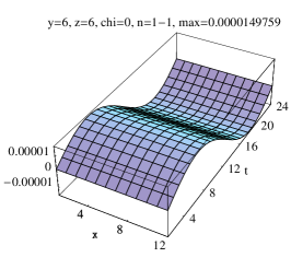
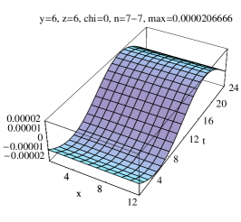
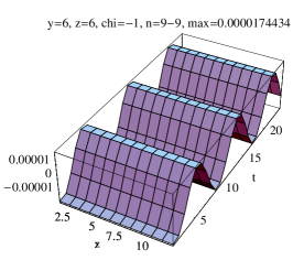
Figure 3: Chiral density of the low-lying eigenmodes of the free overlap Dirac operator: $\rho_{5}\#1$ (left), $\rho_{5}\#7$ (center) $\rho_{5}\#9$ (right). The modes clearly show the plane wave behavior with oscillations of $2p_{\mu}$ (see text).

III.2 Zero Modes and Instantons

An instanton field gives rise to an exact zero mode (the precise expression is given in e.g. Diakonov:2002fq ). Its probability density

$$\rho(x)=\frac{2}{\pi^{2}}\frac{R^{2}}{(x-x_{0})^{2}+R^{2}}$$ (18)

is localized at the instanton core $x_{0}$, with a half-radius of the instanton parameter $R$. Since the zero mode is exactly chiral, its chiral density $\psi^{\dagger}\gamma_{5}\psi$ equals $\pm\rho$. In the instanton liquid model the near-zero modes originate from the overlap of the would-be zero modes carried by individual instantons and anti-instantons. If the overlap is not too large, one expects that the resulting near-zero modes still exhibit definite chirality locally. This picture predicts characteristic properties of the low-lying modes Horvath:2002gk :

• Their probability density should be clearly peaked, indicating the location of instantons.

• The local chirality at the peaks should match the sign of the topological charge and the size of the chiral lump should be correlated to the extension of the topological structure.

• As an instanton and an anti-instanton approach each other, the eigenvalues should be shifted further away from zero and the localization and local chirality properties should fade.

Numerical evidence supporting these assumptions about the local chirality structure of the low-lying Dirac modes are presented in e.g. Edwards:1999dc ; DeGrand:2000gq ; Edwards:2001nd . Here we want to analyze these issues for center vortices.

III.3 Zero Modes and Center Vortices

Reinhardt et al. Reinhardt:2002cm analytically calculate the exact zero modes of the Dirac operator in the background of plane vortices, both non-intersecting and perpendicularly intersecting ones, for an Abelian $U(1)$ gauge field on $\mathbbm{R}^{2},\mathbbm{R}^{4},\mathbbm{T}^{2}$ and $\mathbbm{T}^{4}$. The first vortex field of interest consists of two (anti-)parallel fluxes on a two-torus. Because of a two-dimensional translation symmetry we can identify this with the four-dimensional configuration of a single vortex pair presented in Sec. II.1. The second example contains four flat vortices on a four-torus, which intersect orthogonally in four points. This corresponds to the configuration shown in Fig. 2a.

We want to discuss the boundary conditions used in Reinhardt:2002cm . The four-dimensional problem can be reduced to two two-dimensional ones because of the translation invariance parallel to the vortex sheets. It therefore suffices to deal with the $\mathbbm{T}^{2}$ case. The boundary conditions for a gauge field on $\mathbbm{T}^{2}$ are specified by the two transition functions $\Omega_{x},\Omega_{y}$. In a suitable gauge, it is possible to set $\Omega_{x}=1$. The co-cycle condition then turns into a periodicity condition

$$\Omega_{y}(x+L_{x})=\Omega_{y}(x)$$ (19)

for $\Omega_{y}(x)$, which lives only at the boundary of the rectangle which represents the torus. Therefore $\Omega_{y}$ defines a function $S^{1}\to S^{1}$ belonging to a class of the homotopy group $\pi_{1}(S^{1})\simeq\mathbbm{Z}$. Its winding number $n$ determines the magnetic flux through the $xy$-plane by

$$\Phi:=\oint A_{\mu}\text{d}x_{\mu}=2\pi n\,.$$ (20)

To prove this, we simply perform the line integral over the boundary of the rectangle resulting from cutting up the torus. We set $\Omega_{y}(x)=\exp\{i\chi(x)\}$. Since $\Omega_{y}$ is periodic, $\chi(x+L_{x})=\chi(x)+2\pi n$. Then

$$\Phi =\int_{0}^{L_{x}}A_{x}(x,0)\text{d}x+\int_{0}^{L_{y}}A_{y}(L_{x},y)\text{d}y-\int_{0}^{L_{x}}A_{x}(x,L_{y})\text{d}x-\int_{0}^{L_{y}}A_{y}(0,y)\text{d}y$$

$$=\int_{0}^{L_{x}}A_{x}(x,0)\text{d}x+\int_{0}^{L_{y}}A_{y}(0,y)\text{d}y-\int_{0}^{L_{x}}[A_{x}(x,0)-\partial_{x}\chi(x)]\text{d}x-\int_{0}^{L_{y}}A_{y}(0,y)\text{d}y$$

$$=\int_{0}^{L_{x}}\partial_{x}\chi(x)\text{d}x=\chi(L_{x})-\chi(0)=2\pi n\,.$$ (21)

Consequently, the flux on $\mathbbm{T}^{2}$ is quantized. Note that this would not hold for SU(2) since $\pi_{1}(S^{3})=1$. To create two vortices which carry a flux of $+\pi$ each, Reinhardt et al. use $\Omega_{y}=\exp\{2\pi ix\}$. Returning finally to the fermion field, it obeys boundary conditions consistent with gauge invariance,

$$\psi(x,y+L_{y})=\Omega_{y}(x)\psi(x,y)\,.$$ (22)

In Hollwieser:2011uj we analyzed the zero modes for plane vortex configurations and found good agreement with the results obtained by Reinhardt et al. Reinhardt:2002cm . The discrepancies discussed in our work originate in the finite thickness of our vortex configurations because of finite lattice sizes.

We conclude this section with a quick discussion of the eigenvalues for the spherical vortex. As already mentioned, there always occurs exactly one zero mode, a positive chirality one for the spherical vortex and a negative chirality zero mode for the anti-vortex. The lowest nonzero modes can be seen as some sort of modified eigenmodes of the free Dirac operator. This point of view is motivated by the results presented in Fig. 4a. In this diagram, one can see the eigenvalues for configurations with vortices of the same size in lattice units but different spatial $N_{sp}$ and temporal $N_{t}$ lattice extents. In other words, the vortex gets smaller while the lattice gets finer. One sees from the figures, that the nonzero eigenvalues converge to eigenvalues of the free Dirac operator as the vortex gets smaller and smaller. For the investigated eigenvalues, there seems to be a one to one correspondence between the eigenvalues of the free Dirac operator and the nonzero eigenvalues of the Dirac operator for the vortex configuration. The zero mode is not a lowered nonzero mode, it occurs in addition to the low lying modes. Because the total number of eigenmodes only depends on the lattice size, the number of complex eigenvalues is lowered by two (because of the zero and the doubler mode) for the vortex configuration in comparison to the free case. Note that we still can have a one to one correspondence between all the complex eigenvalues for the vortex and the free case. One can see this by remembering that the correspondence is established in the limit of an infinitely large lattice.

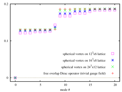
a) b)

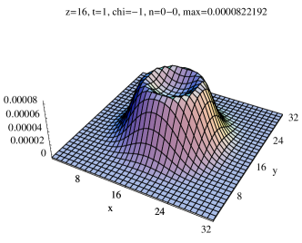
Figure 4: a) The lowest eigenvalues for the spherical vortex with $R=d=3a$ compared to the eigenvalues of the free Dirac operator (red crosses). Eigenvalues are calculated on a $12^{3}\times 6$ lattice with relative lattice constant $a=2$ (magenta boxes), on a $16^{3}\times 8$ lattice with $a=\frac{3}{2}$ (blue stars) and on a $24^{3}\times 12$ lattice with $a=1$ (green crosses). The multiplicity of $\lambda\#1$ is eight, of $\lambda\#2$ 48. b) Spatial distribution of the zero mode, mainly located at the vortex core.

IV Interactions between topological objects

We want to discuss the Dirac equation for a gauge field $\mathcal{A}_{\mu}=\mathcal{A}_{1\mu}+\mathcal{A}_{2\mu}$ consisting of two fields $\mathcal{A}_{1\mu}$ and $\mathcal{A}_{2\mu}$ which are separated in Euclidean space and have non-vanishing topological charge $Q_{i}$. Therefore, the Dirac operators $D_{1}$ for $\mathcal{A}_{1\mu}$ alone and $D_{2}$ for $\mathcal{A}_{2\mu}$ alone would have at least one zero mode. In the following, the zero modes of $D_{1}$ and $D_{2}$ will be called would-be zero modes. Lets discuss the case in which $\mathcal{A}_{1\mu}$ has $Q_{1}=1$ and $\mathcal{A}_{2\mu}$ has $Q_{2}=-1$. For simplicity we assume that $D_{1}$ has only one left handed zero mode $\mid\psi_{1}\rangle$ and $D_{2}$ only one right handed zero mode $\mid\psi_{2}\rangle$. Clearly, these two would-be zero modes are orthogonal and can be part of an orthogonal basis. Let us now have a look at the Dirac operator in this orthogonal basis. In particular we are interested in the upper left $2\times 2$ block

$$\begin{pmatrix}\langle\psi_{1}\mid D\mid\psi_{1}\rangle&\langle\psi_{1}\mid D\mid\psi_{2}\rangle\\ \langle\psi_{2}\mid D\mid\psi_{1}\rangle&\langle\psi_{2}\mid D\mid\psi_{2}\rangle\end{pmatrix}$$ (23)

of the Dirac matrix. The continuum Dirac operator $D$ is given by

$$\begin{split}D&=\gamma_{\mu}\ \left(\partial_{\mu}+\mbox{i}\mathcal{A}_{\mu}(x)\right)=\gamma_{\mu}\ \left(\partial_{\mu}+\mbox{i}\mathcal{A}_{1\mu}(x)+\mbox{i}\mathcal{A}_{2\mu}(x)\right)\\ &=D_{1}+\gamma_{\mu}\mbox{i}\mathcal{A}_{2\mu}(x)=D_{2}+\gamma_{\mu}\ \mbox{i}\mathcal{A}_{1\mu}(x)\,.\end{split}$$ (24)

The first element of (23) therefore evaluates to

$$\langle\psi_{1}\mid D\mid\psi_{1}\rangle=\langle\psi_{1}\mid D_{1}\mid\psi_{1}\rangle+\langle\psi_{1}\mid\gamma_{\mu}\ \mbox{i}\mathcal{A}_{2\mu}(x)\mid\psi_{1}\rangle=0\,.$$ (25)

One can see that $\langle\psi_{1}\mid\gamma_{\mu}\ \mbox{i}\mathcal{A}_{2\mu}(x)\mid\psi_{1}\rangle$ vanishes from

$$\begin{split}\langle\psi_{1}\mid\gamma_{\mu}\ \mbox{i}\mathcal{A}_{2\mu}(x)\mid\psi_{1}\rangle&=\langle\psi_{1}\mid\gamma_{\mu}\ \mbox{i}\mathcal{A}_{2\mu}(x)\ {\gamma_{5}}^{2}\mid\psi_{1}\rangle\\ &=-\ \langle\psi_{1}\mid\gamma_{5}\ \gamma_{\mu}\ \mbox{i}\mathcal{A}_{2\mu}(x)\ {\gamma_{5}}\mid\psi_{1}\rangle=-\ \langle\psi_{1}\mid\gamma_{\mu}\ \mbox{i}\mathcal{A}_{2\mu}(x)\mid\psi_{1}\rangle\ ,.\end{split}$$ (26)

In the same way one can prove

$$\langle\psi_{2}\mid D\mid\psi_{2}\rangle=0\,.$$ (27)

Let us now calculate the off-diagonal terms. The first off-diagonal term evaluates to

$$\langle\psi_{1}\mid D\mid\psi_{2}\rangle=\langle\psi_{1}\mid D_{2}\mid\psi_{2}\rangle+\langle\psi_{1}\mid\gamma_{\mu}\ \mbox{i}\mathcal{A}_{1\mu}(x)\mid\psi_{2}\rangle=0+c=c\,.$$ (28)

Here $c$ stands for the overlap integral $\langle\psi_{1}\mid\gamma_{\mu}\ \mbox{i}\mathcal{A}_{1\mu}(x)\mid\psi_{2}\rangle$. In general, $c$ will be large for eigenmodes that overlap a lot, and small for eigenmodes that overlap only a little. Note that it is crucial that $\mid\psi_{1}\rangle$ and $\mid\psi_{2}\rangle$ have different chirality. Otherwise, by the same argument as used in (26), the overlap integral would have to vanish. The second off-diagonal term of the upper-left $2\times 2$ block is

$$\langle\psi_{2}\mid D\mid\psi_{1}\rangle=\left(\langle\psi_{1}\mid D^{\dagger}\mid\psi_{2}\rangle\right)^{*}=\left(-\ \langle\psi_{1}\mid D\mid\psi_{2}\rangle\right)^{*}=-c^{*}\,.$$ (29)

Here it was used that the continuum Dirac Operator $D$ is anti-hermitian, i.e., $D^{\dagger}=-D$.

Combining (25), (27), (28) and (29), the upper left $2\times 2$ block of the Dirac matrix reads

$$\begin{pmatrix}0&c\\ -c^{*}&0\end{pmatrix}\,.$$ (30)

This $2\times 2$ block can easily be diagonalized. The eigenvalues $\lambda_{1,2}$ and the normalized eigenvectors $\psi^{\prime}_{1,2}$ of (30) are

$$\lambda_{1,2}=\pm\mbox{i}\sqrt{cc^{*}}=\pm\mbox{i}|c|,\quad\psi^{\prime}_{1,2}=\frac{1}{\sqrt{2}}\begin{pmatrix}\pm\mbox{i}\sqrt{\frac{c}{c^{*}}}\\ 1\end{pmatrix}\,.$$ (31)

This means that the interaction transforms the two (would-be) zero modes into two near-zero modes. Those near-zero modes also occur additionally to the free Dirac eigenmodes and therefore we still enumerate them like zero modes by #0. The strength of the interaction quantified by the overlap integral $c$ determines the size of the near-zero eigenvalue. Note that the new near-zero modes consist in equal parts of the would-be zero modes $\mid\psi_{1}\rangle$ and $\mid\psi_{2}\rangle$. Therefore the scalar and chiral densities of the near-zero modes are simply an average of the densities of the would-be zero modes.

So far we have ignored everything except the upper left $2\times 2$ block of the Dirac matrix. To get exact eigenmodes we clearly have to diagonalize the whole Dirac matrix and not only this $2\times 2$ block. However, (31) represents a legitimate approximation to the exact eigenvalues and eigenmodes if the elements of the form

$$\langle\psi_{j}\mid D\mid\psi_{1,2}\rangle=\langle\psi_{j}\mid\gamma_{\mu}\ \mbox{i}\mathcal{A}_{2,1\mu}(x)\mid\psi_{1,2}\rangle\quad\mbox{with}\quad j>2$$

are a lot smaller than the overlap integral $c=\langle\psi_{1}\mid\gamma_{\mu}\ \mbox{i}\mathcal{A}_{1\mu}(x)\mid\psi_{2}\rangle$. Usually this will be the case, because $\mid\psi_{1}\rangle$ is localized at $\mathcal{A}_{1\mu}$ and $\mid\psi_{j}\rangle$ with $j>2$ is not. Let us also have a quick look at what happens when we have two would-be zero modes with the same chirality. In this case also the off-diagonal terms of the upper left $2\times 2$ matrix vanish and the would-be zero modes are actual zero modes.

Note that the mechanism discussed in this section is the basis for the instanton liquid model of spontaneous chiral symmetry breaking (see Diakonov:2002fq for a detailed review). In the instanton liquid model the QCD-vacuum consists of an ensemble of instantons and anti-instantons whose would-be zero modes split into near-zero modes because of interactions. Therefore, one gets a non-vanishing eigenmode density around zero, which gives via the Banks-Casher relation a finite chiral condensate and broken chiral symmetry. Clearly, one can construct such a model also with other topological objects, as will be shown in the next section for center vortices.

V Vortices and $\chi$SB

In Sec. II we discussed the various possibilities of vortices to create topological charge, i.e., via writhing and intersection points as well as through their color structure. In previous works we presented results on the attraction of zero modes for flat Hollwieser:2011uj and spherical Jordan:2007ff ; Hollwieser:2010mj ; Hollwieser:2012kb ; Schweigler:2012ae vortex configurations. Here we present some results on how vortices form near-zero modes from would-be zero modes through interactions.

V.1 Spherical Vortices and Instantons

We start with spherical vortices and show that their effects on fermions is pretty much the same as those of instantons. We have shown in Fig. 4 that they attract a zero mode and its scalar density peaks at the vortex surface. We interpreted the nonzero modes as eigenmodes of the free Dirac operator, which are shifted slightly because of their interaction with the nontrivial gauge field content. In Fig. 5a we see that a single instanton has nearly exactly the same eigenvalues as a single spherical vortex. In Fig. 6 we show that even the chiral densities of the lowest eigenmodes distribute similarly, except for the fact that the response of the fermions to the spherical vortex is squeezed in the time direction, since the vortex is localized in a single time slice ($t=5$). Another interesting issue is that the nonzero eigenmodes show nice plane wave oscillations, like the free eigenmodes in Fig. 3, mode #8 however shows some similarity to the zero mode, its eigenvalue is also clearly enhanced compared to the free spectrum. This is only a side remark however, as we are not sure how to interpret this and it does not seem to be important for the creation of near-zero modes since we observe the same effect for instantons.

We further plot the spectra of instanton–anti-instanton, spherical vortex–anti-vortex and instanton–anti-vortex pairs in Fig. 5a. We again see nearly exactly the same eigenvalues for instanton or spherical vortex pairs, but now we get instead of two would-be zero modes a pair of near-zero modes for each pair. The chiral density plots in Fig. 7 for the instanton–anti-instanton pair and Fig. 8 for the spherical vortex–anti-vortex pair show, besides the similar densities, that the near-zero mode is a result of two chiral parts corresponding to the two constituents of the pairs. The nonzero modes can again be identified with the free overlap modes with the same side remark for mode #8. In Fig. 5b we plot the eigenvalues of two (anti-)instantons and two spherical (anti-)vortices giving topological charge $Q=2$ ($Q=-2$) and therefore two zero modes, two vortex–anti-vortex pairs with two near-zero modes and a configuration with two vortices and an anti-vortex (i.e., a single vortex plus one vortex–anti-vortex pair) giving one zero mode ($Q=1$) and one near-zero mode. The chiral densities for the last configuration in Fig. 9 show that the zero mode peaks at both spherical vortices, the near-zero mode again consists of two chiral parts from the (second/would-be) zero mode of the two vortices and the (would-be) zero mode of the anti-vortex. Now the modes #7 and #8 clearly deviate from the free eigenvalues showing similar densities as the zero and the near-zero mode respectively.

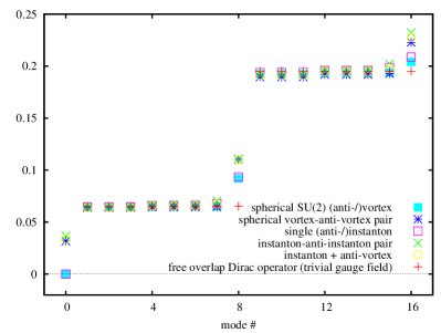
a) b)

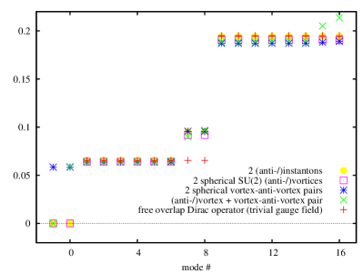
Figure 5: The lowest overlap eigenvalues for instanton and spherical vortex configurations compared to the eigenvalues of the free (overlap) Dirac operator.

a)
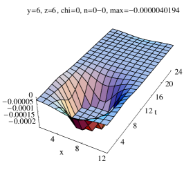
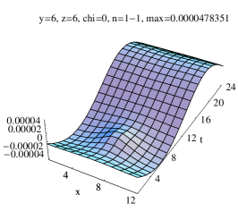
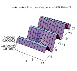
b)
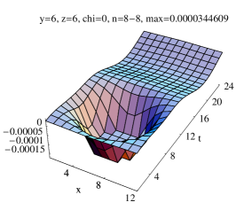
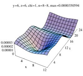
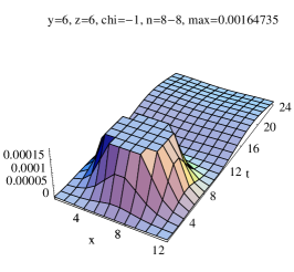
c)
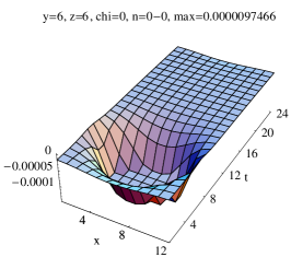
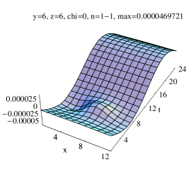
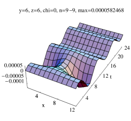
d)

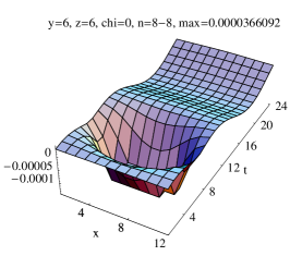
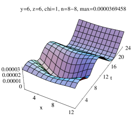
Figure 6: Chiral densities of overlap eigenmodes: a) zero mode (left), first (center), ninth (right) and b) eighth ($\rho_{5}$ left, $\rho_{+}$ center and $\rho_{-}$ right) nonzero modes for an instanton; c) and d) the same as a) and b) but for a spherical vortex.

a)
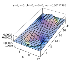
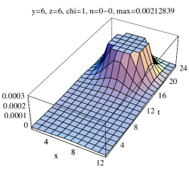
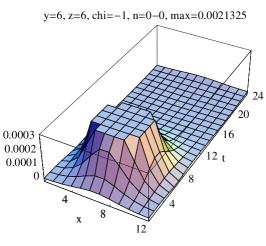
b)
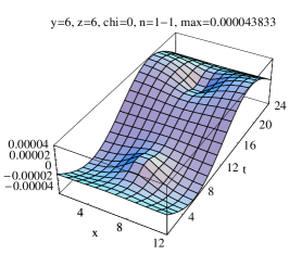
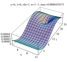
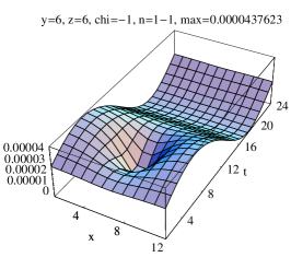
c)
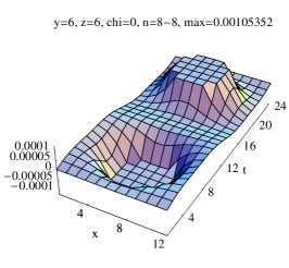
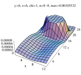
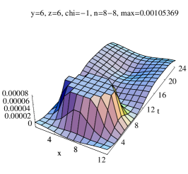
d)

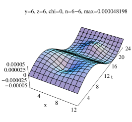
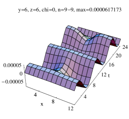
Figure 7: Chiral densities ($\rho_{5}$ left, $\rho_{+}$ center and $\rho_{-}$ right column) of the a) lowest (near-zero), b) second-lowest (nonzero) and c) eighth (nonzero) eigenmode of the overlap Dirac operator for an instanton–anti-instanton pair. d) $\rho_{5}$ of the sixth (left), seventh (center) and ninth (right) eigenmode.

a)
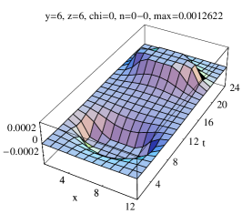
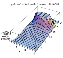
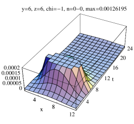
b)
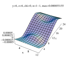
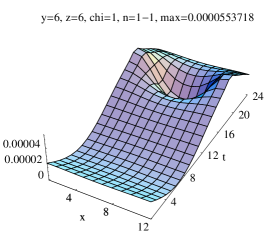
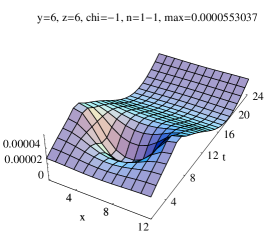
c)
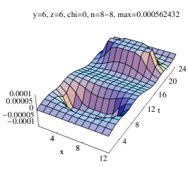
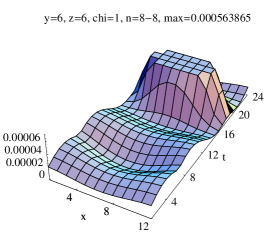
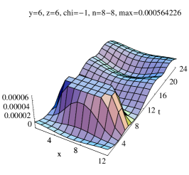
d)

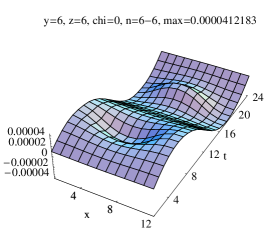
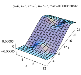
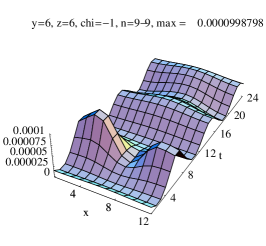
Figure 8: Same as Fig. 7 but for a spherical vortex–anti-vortex pair. Chiral densities ($\rho_{5}$ left, $\rho_{+}$ center and $\rho_{-}$ right column) of the a) lowest (near-zero), b) second-lowest (nonzero) and c) eighth (nonzero) eigenmode. d) $\rho_{5}$ of the sixth (left), seventh (center) and ninth (right) eigenmode.

a)
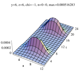
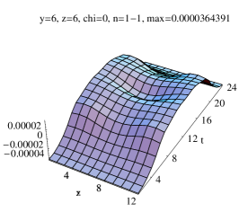
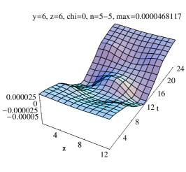
b)
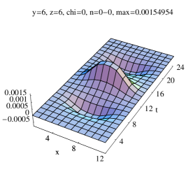
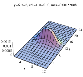
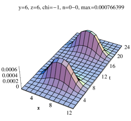
c)
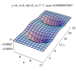
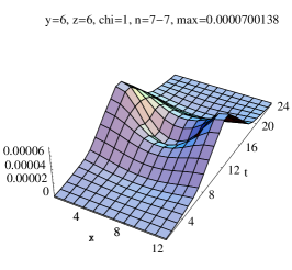
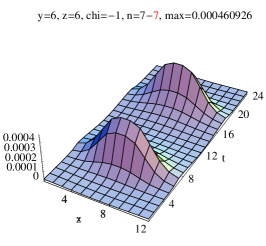
d)

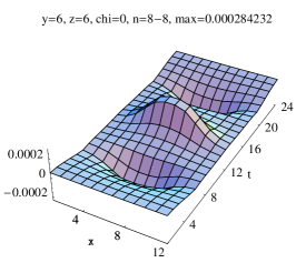
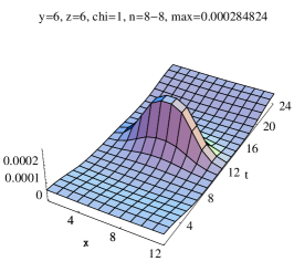
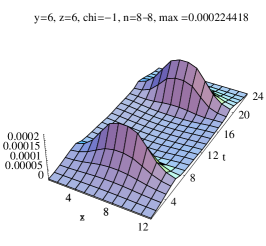
Figure 9: Chiral densities of overlap eigenmodes for spherical vortices at $t=4$ and $t=20$ and an anti-vortex at $t=12$: a) zero mode $\rho_{-}\#0-$ (left), $\rho_{5}\#1$ (center) and $\rho_{5}\#5$ (right). b) near-zero (second-lowest) mode #0, c) #7 ($\approx\#0-$) and d) #8 ($\approx\#0$) with $\rho_{5}$ (left), $\rho_{+}$ (center) and $\rho_{-}$ (right).

Finally we want to analyze the effect of the distance between vortex and anti-vortex. In Fig. 10a) we plot the low-lying eigenvalues for a spherical vortex–anti-vortex pair with varying distance in time direction. The near-zero mode is clearly shifted away from zero as the vortex and anti-vortex approach each other. If they lie in neighboring time slices (i.e. t=3 and t=4) the Dirac operator cannot resolve them as individual objects, i.e. the eigenmodes overlap heavily and no near-zero mode is produced. This can also be seen from the plane wave behavior in the chiral density of the lowest eigenmode in Fig. 10b). The chiral densities of the near-zero modes for vortex–anti-vortex pairs with distances 2, 3, and 4 are shown in Fig. 11, they show no plane wave behavior and an increasing degree of local chirality. From the density plots we conclude that the eigenmode peaks at the spherical vortices extend over 3-4 time slices. Hence we expect the overlap of the modes to vanish if the vortex and anti-vortex are separated by 5-6 time slices and indeed we see that the eigenvalues do not change significantly if we increase the distance further. Thus, the spherical vortices reproduce all characteristic properties of low-lying modes for chiral symmetry breaking given in Horvath:2002gk and summarized at the end of section III.2. The results clearly show that we may draw the same conclusions for spherical vortices as for instantons concerning the creation of near-zero modes.

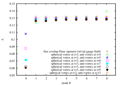
a) b)

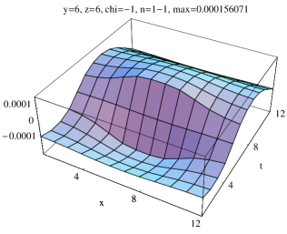
Figure 10: a) The lowest overlap eigenvalues for spherical vortex–anti-vortex pairs with varying distance compared to the eigenvalues of the free (overlap) Dirac operator. b) Chiral density of the lowest overlap eigenmode for spherical vortex and anti-vortex in neighboring time slices (t=3 and t=4). Its plane wave behavior shows that this eigenmode is not a near-zero mode and hence it appears as mode #1 in a).

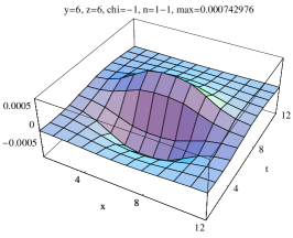
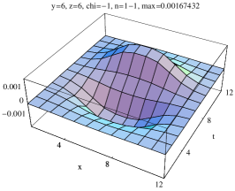
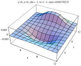
Figure 11: Chiral density of the overlap near-zero mode for a spherical vortex at t=3 and an anti-vortex at t=5, t=7 and t=9.

V.2 Planar vortex configurations

For plane vortices the situation is more complicated, as we do not get single, localized lumps of topological charge $Q=\pm 1$, which would attract single zero modes. We rather deal with vortex intersection points each contributing with $Q=\pm 1/2$ and only attracting zero modes as combinations of topological charge contributions. Recall from Fig. 9a, that even for two spherical vortices and one anti-vortex the corresponding zero mode cannot be matched to a single vortex, but the zero mode belongs to both topological charge contributions. As shown in Fig. 1a and c one can get two different values of topological charge $Q$ for two pairs of planar vortex surfaces, intersecting in four points. For parallel flux direction we get two real zero modes, according to the total topological charge $Q=\pm 2$. These modes we analyzed in Hollwieser:2011uj , they peak at least at two of the four topological charge contributions of $Q=1/2$. For pairs of planar vortex surfaces with opposite (anti-parallel) flux directions we get $Q=0$ according to the topological charge contributions in Fig. 1c and four real near-zero modes. The sum of local chiralities of these four modes peaks at the intersection points according to the sign of the local topological charge, as shown in Fig. 12b. Fig. 13 shows that every near-zero mode is concentrated on two intersections with opposite topological charge contribution. The number of near-zero modes seems to be related to the four possible combinations to get topological charge $Q=0$ from two of the four $Q=\pm 1/2$ contributions. The non-zero modes again show plane wave oscillations.

The presented results are obtained for the usual anti-periodic boundary conditions in the time-direction and periodic boundary conditions in the spatial directions. However, we want to emphasize that the number of (near-) zero modes does not change with respect to boundary conditions, even if we impose anti-periodic boundary conditions in all directions. The reason it is important to ascertain this is that plane vortex pairs by themselves are somewhat special, as they can attract zero modes already on their own according to their magnetic flux, due to their essentially two-dimensional nature (see Sec. III.3 and Reinhardt et al. Reinhardt:2002cm ). For periodic boundary conditions we get for a single pair of planar vortex surfaces with the same (parallel) flux direction two non-chiral zero modes. They have the same chirality peaking at the two vortices, see Fig. 14a and compare to Fig. 1 in  Reinhardt:2002cm . In fact, these modes are remnants of the trivial gauge fields, where one gets four non-chiral zero modes for periodic boundary conditions. The two ”missing” zero modes, which would of course have opposite chirality are suppressed by the vortex structure. For a single vortex pair with opposite flux direction (anti-parallel vortices) we get four non-chiral near-zero modes peaking at the two vortices with opposite (local) chiralities (two left-handed and two right-handed), see Fig. 14b. The non-zero modes again show plane wave oscillations, see Fig. 14c. In four dimensions these non-chiral modes can be removed by anti-periodic boundary conditions in at least one of the directions parallel to the vortex flux, i.e., for usual anti-periodic boundary conditions in the time direction the near-zero mode results in this paragraph are only valid for ”spatial” plane vortices, e.g. xy-vortices. For zt-vortices there are no (near-) zero modes, as there are none for anti-periodic boundary conditions in the z-direction and in the case of xy-vortices with anti-periodic boundary conditions in the x or y-direction. Since the (near-) zero modes induced by single pairs of planar vortices can be removed by appropriate boundary conditions, but they persist for two intersecting vortex pairs regardless of boundary conditions, we conclude that indeed the intersections by themselves can cause near-zero modes.

Now, the mechanism of Sec. V.1 or the analog instanton liquid model does not directly apply to the case of planar vortices, since there are no localized lumps of topological charge $Q=\pm 1$. Nevertheless the vortices attract chiral (near-)zero modes via their intersections with topological charge $Q=\pm 1/2$, similar to the case of merons Reinhardt:2001hb and calorons Bruckmann:2009pa . We conclude that the color structure of vortices and their intersection points are able to create a finite density of near-zero modes and break chiral symmetry via the Banks-Casher relation.

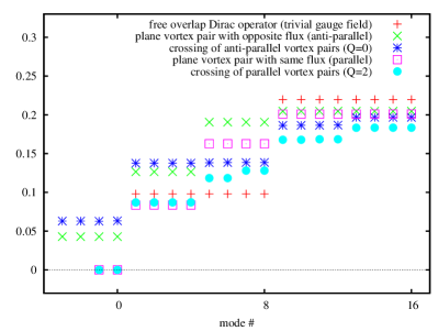
a) b)

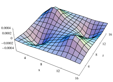
Figure 12: a) The lowest overlap eigenvalues for plane vortex configurations compared to the eigenvalues of the free (overlap) Dirac operator (red crosses). Note that the low-lying eigenvalues for single vortex pairs (green crosses and magenta boxes) only occur for appropriate boundary conditions (see text for details). b) Chiral density $\rho_{5}\#0$ in the intersection plane of all four near-zero modes of crossing flat vortex pairs with opposite flux direction ($Q=0$).

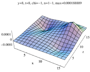
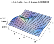
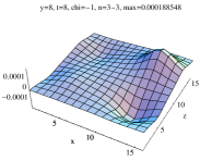
a) b) c) d)

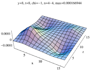
Figure 13: The individual modes of Fig. 12b are mainly localized at two neighboring intersection points with opposite topological charge contributions: a) mode #1 mainly peaks at the intersections in the back at $z=12$, b) mode #2 is mainly localized at the intersections to the left ($x=4$), c) mode #3 at $x=12$ (right) and d) mode #4 at $z=4$ (front).

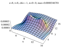
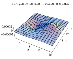
a) b) c)

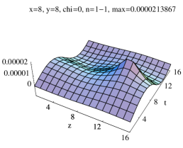
Figure 14: Chiral densities of the low-lying eigenmodes of the overlap Dirac operator for plane vortices: a) two zero modes of one parallel vortex pair, i.e., two vortices with the same flux direction, b) four near-zero modes and c) first nonzero mode of one anti-parallel vortex pair, i.e., two vortices with opposite flux direction. Note that the modes in a) and b) are only present for periodic boundary conditions in directions parallel to the vortex flux (see text for details).

V.3 Asqtad Staggered Modes

For completeness we shortly discuss the asqtad staggered eigenmodes for the presented configurations (see Figs. 15, 16, 17, 18, 19). In principle the same conclusions as for overlap modes apply if we consider the double degeneracy of asqtad staggered modes due to charge conjugation. Hence we have two (would-be) zero modes for $Q=\pm 1$ and there are four times as many near-zero modes since two would-be zero modes do result in two pairs of near-zero modes instead of one for overlap modes. Remember that for a single pair of plane vortices with parallel flux the overlap operator finds two non-chiral zero modes. It is interesting to note, that the staggered operator identifies them as non-chiral near-zero modes as indicated by their number and chiralities (magenta boxes in Fig. 16). The non-chiral modes for single vortex pairs can again be removed by anti-periodic boundary conditions in directions parallel to the vortex flux. The chirality of the asqtad staggered eigenmodes is given by $\langle\psi\gamma_{5}\psi\rangle$, where $\gamma_{5}$ corresponds to a displacement along the diagonal of a hypercube. Staggered fermions do not have exact zero modes, but a separation between would-be and non-zero modes is observed for improved staggered quark actions Wong:2004ai . The plots show that the would-be and near-zero modes have enhanced chirality compared to nonzero modes and we even observe the local chiral density properties for the near-zero modes which we discussed for the overlap modes.

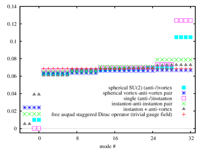
a) b)

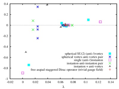
Figure 15: The lowest asqtad staggered eigenvalues for instanton and spherical vortex configurations compared to the eigenvalues of the free Dirac operator. b) Chirality of the corresponding eigenmodes.

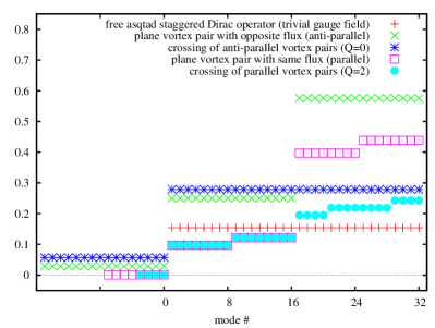
a) b)

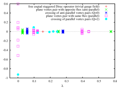
Figure 16: a) The lowest asqtad staggered eigenvalues for plane vortex configurations compared to the eigenvalues of the free Dirac operator. b) Chirality of the corresponding eigenmodes. Again, the low-lying eigenmodes for single vortex pairs (green crosses and magenta boxes) only occur for appropriate boundary conditions (see text for details).

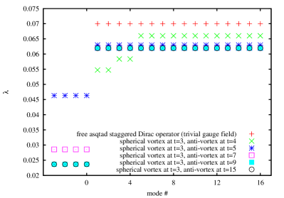
a) b)

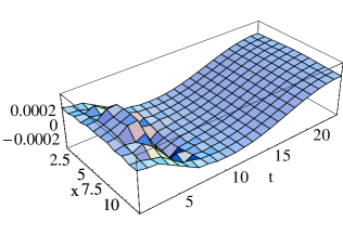
Figure 17: a) The lowest asqtad staggered eigenvalues for spherical vortex–anti-vortex pairs with varying distance compared to the eigenvalues of the free (overlap) Dirac operator. b) Chiral density of the lowest asqtad staggered eigenmode for spherical vortex and anti-vortex in neighboring time slices (t=3 and t=4).

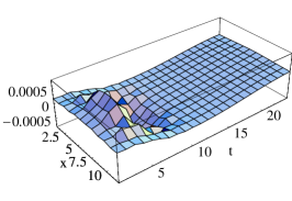
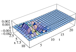
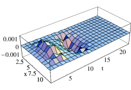
Figure 18: Chiral density of the asqtad staggered near-zero mode for a spherical vortex in time slice t=3 and an anti-vortex in a) t=5, b) t=7 and c) t=9.

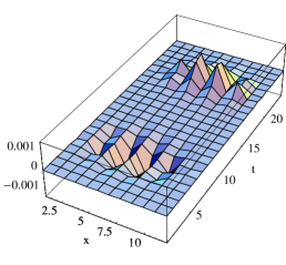
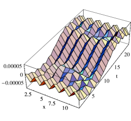
a) b) c)

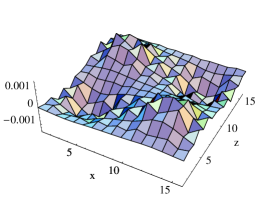
Figure 19: Chiral densities of the low-lying eigenmodes of the asqtad staggered Dirac operator: a) four near-zero and b) nonzero modes of a spherical vortex–anti-vortex pair, and c) 16 near-zero modes of the crossing flat vortex pairs in Fig. 12b).

VI Conclusions

The instanton liquid model provides a physical picture of chiral symmetry breaking via the idea of quarks “hopping” between random instantons and anti-instantons, changing their helicity each time. This process can be described by quarks propagating between quark-instanton vertices. As fermions do not seem to make much of a difference between instantons and spherical vortices this picture can be extended to colorful spherical center vortices. In fact, the spherical vortices reproduce all characteristic properties of low-lying modes for chiral symmetry breaking Horvath:2002gk :

• Their probability density is clearly peaked at the location of the vortices.

• The local chirality at the peaks exactly matches the sign of the topological charge and the size of the chiral lump is correlated to the extension of the topological structure.

• As a spherical vortex and an anti-vortex approach each other, the eigenvalues are shifted further away from zero and the localization and local chirality properties fade.

In the vortex picture the model of chiral symmetry breaking can be formulated even more generally, as we have shown that various shapes of vortices attract (would-be) zero modes which contribute via interactions to a finite density of near-zero modes with local chiral properties, i.e., local chirality peaks at corresponding topological charge contributions. The simple picture of localized would-be zero modes from the instanton liquid model or spherical vortex configurations as discussed in Sec. IV and V.1 does not apply directly to general vortex structures as there are not only topological charge contributions of $Q=\pm 1$. In Monte Carlo configurations we do not, of course, find perfectly flat or spherical vortices, as one does not find perfect instantons. The general picture of topological charge from vortex intersections, writhing points and even color structure contributions or instantons can provide a general picture of $\chi$SB: any source of topological charge can attract (would-be) zero modes and produce a finite density of near-zero modes leading to chiral symmetry breaking via the Banks-Casher relation. Here one also has to ask what could be the dynamical explanation of $\chi$SB. We can try the conjecture that only a combination of color electric and magnetic fields leads to $\chi$SB, electric fields accelerating color charges and magnetic fields trying permanently to reverse the momentum directions on spiral shaped paths. Such reversals of momentum keeping the spin of the particles should especially happen for very slowly moving color charges. Alternatively we could argue that magnetic color charges are able to flip the spin of slow quarks, i.e. when they interact long enough with the vortex structures.

Finally, it seems that vortices not only confine quarks into bound states but also change their helicity in analogy to the instanton liquid model. We therefore emphasize that the center vortex model of quark confinement is indeed capable of describing chiral symmetry breaking. While we can not give a conclusive answer to the question of a dynamical explanation for the mechanism of $\chi$SB, we can speculate that the generation of near-zero modes demonstrated for artificial configuration in this paper, carries over to vortices present in Monte Carlo generated configurations. As the near-zero modes are located around intersection and writhing points of vortices that carry topological charge, the behavior away from these points would seem to be far less important.

We conclude by remarking that other mechanisms of chiral symmetry breaking, in addition to the instanton liquid paradigm or the vortex picture described in this paper, may be operative in the Yang-Mills vacuum. For instance, it also seems possible that, even in the absence of would-be zero modes, the random interactions of quarks with the vortex background may be strong enough to smear the free dispersion relation such that a finite Dirac operator spectral density at zero virtuality is generated. In fact, a confining interaction by itself generates chiral symmetry breaking, independent of any particular consideration of would-be zero modes connected to topological charge Casher:1979vw . However, this effect on its own is not sufficiently strong for a quantitative explanation of the chiral condensate; other effects, among them possibly the ones considered in this article, must play a role. Also, the importance of the long-range nature of low-dimensional topological structures for the understanding of the mechanism of $\chi$SB in QCD was underlined by various results of different groups Horvath:2002zy ; Horvath:2003is ; Bowman:2010zr ; Braguta:2010ej ; OMalley:2011aa ; Buividovich:2011mj ; O'Malley:2011zz ; Braguta:2013kpa , and agrees well with a vortex picture of $\chi$SB.

- (1) A. A. Belavin, A. M. Polyakov, A. S. Schwartz, and Y. S. Tyupkin, “Pseudoparticle solutions of the Yang-Mills equations,” Phys. Lett. B59 (1975) 85–87.
- (2) A. Actor, “Classical Solutions of SU(2) Yang-Mills Theories,” Rev. Mod. Phys. 51 (1979) 461.
- (3) G. ’t Hooft, “Computation of the quantum effects due to a four- dimensional pseudoparticle,” Phys. Rev. D 14 (1976) 3432–3450.
- (4) C. W. Bernard, “Gauge zero modes, instanton determinants, and quantum- chromodynamic calculations,” Phys. Rev. D 19 (1979) 3013.
- (5) M. F. Atiyah and I. M. Singer, “The Index of elliptic operators. 5,” Annals Math. 93 (1971) 139–149.
- (6) A. S. Schwarz, “On Regular Solutions of Euclidean Yang-Mills Equations,” Phys. Lett. B67 (1977) 172–174.
- (7) L. S. Brown, R. D. Carlitz, and C.-k. Lee, “Massless Excitations in Instanton Fields,” Phys. Rev. D 16 (1977) 417–422.
- (8) R. Narayanan and H. Neuberger, “A construction of lattice chiral gauge theories,” Nucl. Phys. B443 (1995) 305–385, arXiv:9411108 [hep-th].
- (9) E.-M. Ilgenfritz and M. Muller-Preussker, “Statistical Mechanics of the Interacting Yang-Mills Instanton Gas,” Nucl. Phys. B184 (1981) 443.
- (10) D. Diakonov and V. Y. Petrov, “Chiral Condensate in the Instanton Vacuum,” Phys. Lett. B147 (1984) 351–356.
- (11) D. Diakonov and V. Y. Petrov, “MESON CURRENT CORRELATION FUNCTIONS IN INSTANTON VACUUM,” Sov.Phys.JETP 62 (1985) 431–437.
- (12) G. ’t Hooft, “On the phase transition towards permanent quark confinement,” Nucl. Phys. B138 (1978) 1.
- (13) P. Vinciarelli, “Fluxon solutions in nonabelian gauge models,” Phys. Lett. B78 (1978) 485–488.
- (14) T. Yoneya, “Z(n) topological excitations in yang-mills theories: Duality and confinement,” Nucl. Phys. B144 (1978) 195.
- (15) J. M. Cornwall, “Quark confinement and Vortices in massive gauge invariant QCD,” Nucl. Phys. B157 (1979) 392.
- (16) G. Mack and V. B. Petkova, “Comparison of Lattice Gauge Theories with gauge groups Z(2) and SU(2),” Ann. Phys. 123 (1979) 442.
- (17) H. B. Nielsen and P. Olesen, “A Quantum Liquid Model for the QCD Vacuum: Gauge and Rotational Invariance of Domained and Quantized Homogeneous Color Fields,” Nucl. Phys. B160 (1979) 380.
- (18) L. Del Debbio, M. Faber, J. Greensite, and Š. Olejník, “Center dominance and Z(2) vortices in SU(2) lattice gauge theory,” Phys. Rev. D 55 (1997) 2298–2306, arXiv:9610005 [hep-lat].
- (19) K. Langfeld, H. Reinhardt, and O. Tennert, “Confinement and scaling of the vortex vacuum of SU(2) lattice gauge theory,” Phys. Lett. B419 (1998) 317–321, arXiv:9710068 [hep-lat].
- (20) L. Del Debbio, and M. Faber, and J. Greensite, and Š. Olejník, “Center dominance, center vortices, and confinement,” arXiv:9708023 [hep-lat].
- (21) T. G. Kovacs and E. T. Tomboulis, “Vortices and confinement at weak coupling,” Phys. Rev. D 57 (1998) 4054–4062, arXiv:9711009 [hep-lat].
- (22) M. Engelhardt and H. Reinhardt, “Center vortex model for the infrared sector of Yang-Mills theory: Confinement and deconfinement,” Nucl. Phys. B585 (2000) 591–613, arXiv:9912003 [hep-lat].
- (23) R. Bertle and M. Faber, “Vortices, confinement and Higgs fields,” arXiv:0212027 [hep-lat].
- (24) M. Engelhardt, M. Quandt, and H. Reinhardt, “Center vortex model for the infrared sector of SU(3) Yang-Mills theory: Confinement and deconfinement,” Nucl.Phys. B685 (2004) 227–248, arXiv:0311029 [hep-lat].
- (25) P. de Forcrand and M. D’Elia, “On the relevance of center vortices to QCD,” Phys. Rev. Lett. 82 (1999) 4582–4585, arXiv:9901020 [hep-lat].
- (26) C. Alexandrou, P. de Forcrand, and M. D’Elia, “The role of center vortices in QCD,” Nucl. Phys. A663 (2000) 1031–1034, arXiv:9909005 [hep-lat].
- (27) H. Reinhardt and M. Engelhardt, “Center vortices in continuum yang-mills theory,” in Quark Confinement and the Hadron Spectrum IV, W. Lucha and K. M. Maung, eds., pp. 150–162. World Scientific, 2002. arXiv:0010031 [hep-th].
- (28) M. Engelhardt, “Center vortex model for the infrared sector of Yang-Mills theory: Quenched Dirac spectrum and chiral condensate,” Nucl.Phys. B638 (2002) 81–110, arXiv:0204002 [hep-lat].
- (29) V. Bornyakov et al., “Interrelation between monopoles, vortices, topological charge and chiral symmetry breaking: Analysis using overlap fermions for SU(2),” Phys. Rev. D 77 (2008) 074507, arXiv:0708.3335 [hep-lat].
- (30) R. Höllwieser, M. Faber, J. Greensite, U.M. Heller, and Š. Olejník, “Center Vortices and the Dirac Spectrum,” Phys. Rev. D 78 (2008) 054508, arXiv:0805.1846 [hep-lat].
- (31) G. Jordan, R. Höllwieser, M. Faber, U.M. Heller, “Tests of the lattice index theorem,” Phys. Rev. D 77 (2008) 014515, arXiv:0710.5445 [hep-lat].
- (32) R. Höllwieser, M. Faber, U.M. Heller, “Lattice Index Theorem and Fractional Topological Charge,” arXiv:1005.1015 [hep-lat].
- (33) R. Höllwieser, M. Faber, U.M. Heller, “Critical analysis of topological charge determination in the background of center vortices in SU(2) lattice gauge theory,” Phys. Rev. D 86 (2012) 014513, arXiv:1202.0929 [hep-lat].
- (34) T. Schweigler, R. Höllwieser, M. Faber, and U.M. Heller, “Colorful SU(2) center vortices in the continuum and on the lattice,” Phys. Rev. D 87 (2013) 054504, arXiv:1212.3737 [hep-lat].
- (35) T. Banks and A. Casher, “Chiral Symmetry Breaking in Confining Theories,” Nucl. Phys. B169 (1980) 103.
- (36) H. Reinhardt, “Topology of center vortices,” Nucl. Phys. B628 (2002) 133–166, arXiv:0112215 [hep-th].
- (37) R. Bertle, M. Faber, J. Greensite, and Š. Olejník, “The structure of projected center vortices in lattice gauge theory,” JHEP 03 (1999) 019, arXiv:9903023 [hep-lat].
- (38) J. Greensite, “The confinement problem in lattice gauge theory,” Prog. Part. Nucl. Phys. 51 (2003) 1, arXiv:0301023 [hep-lat].
- (39) M. Chernodub, F. Gubarev, M. Polikarpov, and V. I. Zakharov, “Monopoles and confining strings in QCD,” arXiv:0103033 [hep-lat].
- (40) R. Höllwieser, M. Faber, U.M. Heller, “Intersections of thick Center Vortices, Dirac Eigenmodes and Fractional Topological Charge in SU(2) Lattice Gauge Theory,” JHEP 1106 (2011) 052, arXiv:1103.2669 [hep-lat].
- (41) M. Engelhardt and H. Reinhardt, “Center projection vortices in continuum Yang-Mills theory,” Nucl. Phys. B567 (2000) 249, arXiv:9907139 [hep-th].
- (42) T. M. W. Nye and M. A. Singer, “An -Index Theorem for Dirac Operators on ,” arXiv:0009144 [math].
- (43) E. Poppitz and M. Unsal, “Index theorem for topological excitations on and Chern-Simons theory,” JHEP. 0903 (2009) 027, arXiv:0812.2085 [hep-th].
- (44) T. Schweigler, “Topological objects and chiral symmetry breaking in QCD,” Master’s thesis, Vienna University of Technology, 2012.
- (45) R. G. Edwards, U. M. Heller, and R. Narayanan, “A study of practical implementations of the overlap-Dirac operator in four dimensions,” Nucl. Phys. B540 (1999) 457–471, arXiv:9807017 [hep-lat].
- (46) R. G. Edwards, U. M. Heller, and R. Narayanan, “A study of chiral symmetry in quenched QCD using the overlap-Dirac operator,” Phys. Rev. D 59 (1999) 094510, arXiv:9811030 [hep-lat].
- (47) B. Bunk, K. Jansen, B. Jegerlehner, M. Luscher, H. Simma, et al., “A New simulation algorithm for lattice QCD with dynamical quarks,” Nucl.Phys.Proc.Suppl. 42 (1995) 49–55, arXiv:9411016 [hep-lat].
- (48) T. Kalkreuter and H. Simma, “An Accelerated conjugate gradient algorithm to compute low lying eigenvalues: A Study for the Dirac operator in SU(2) lattice QCD,” Comput.Phys.Commun. 93 (1996) 33–47, arXiv:9507023 [hep-lat].
- (49) D. Diakonov, “Instantons at work,” Prog.Part.Nucl.Phys. 51 (2003) 173–222, arXiv:0212026 [hep-ph].
- (50) I. Horvath et al., “Local chirality of low-lying Dirac eigenmodes and the instanton liquid model,” Phys. Rev. D 66 (2002) 034501, arXiv:0201008 [hep-lat].
- (51) R. G. Edwards, U. M. Heller, J. E. Kiskis, and R. Narayanan, “Topology and chiral symmetry in QCD with overlap fermions,” arXiv:9912042 [hep-lat].
- (52) T. A. DeGrand and A. Hasenfratz, “Low lying fermion modes, topology and light hadrons in quenched QCD,” Phys. Rev. D 64 (2001) 034512, arXiv:0012021 [hep-lat].
- (53) R. G. Edwards and U. M. Heller, “Are topological charge fluctuations in QCD instanton dominated?,” Phys. Rev. D 65 (2002) 014505, arXiv:0105004 [hep-lat].
- (54) H. Reinhardt, O. Schroeder, T. Tok, and V. C. Zhukovsky, “Quark zero modes in intersecting center vortex gauge fields,” Phys. Rev. D 66 (2002) 085004, arXiv:0203012 [hep-th].
- (55) H. Reinhardt and T. Tok, “Merons and instantons in laplacian abelian and center gauges in continuum Yang-Mills theory,” Phys. Lett. B505 (2001) 131–140.
- (56) F. Bruckmann, E.-M. Ilgenfritz, B. Martemyanov, and B. Zhang, “The Vortex Structure of SU(2) Calorons,” Phys. Rev. D 81 (2010) 074501, arXiv:0912.4186 [hep-th].
- (57) K. Y. Wong and R. M. Woloshyn, “Topology and staggered fermion action improvement,” Nucl. Phys. Proc. Suppl. 140 (2005) 620–622, arXiv:0407003 [hep-lat].
- (58) A. Casher, “Chiral Symmetry Breaking in Quark Confining Theories,” Phys. Lett. B83 (1979) 395.
- (59) I. Horvath, S. Dong, T. Draper, K. Liu, N. Mathur, et al., “Uncovering low dimensional topological structure in the QCD vacuum,” JLAB-THY-02-69 (2002) 312–314, arXiv:0212013 [hep-lat].
- (60) I. Horvath, S. Dong, T. Draper, F. Lee, K. Liu, et al., “Low dimensional long range topological structure in the QCD vacuum,” Nucl.Phys.Proc.Suppl. 129 (2004) 677–679, arXiv:0308029 [hep-lat].
- (61) P. O. Bowman, K. Langfeld, D. B. Leinweber, A. Sternbeck, L. von Smekal, et al., “Role of center vortices in chiral symmetry breaking in SU(3) gauge theory,” Phys. Rev. D 84 (2011) 034501, arXiv:1010.4624 [hep-lat].
- (62) V. Braguta, P. Buividovich, T. Kalaydzhyan, S. Kuznetsov, and M. Polikarpov, “The Chiral Magnetic Effect and chiral symmetry breaking in SU(3) quenched lattice gauge theory,” Phys.Atom.Nucl. 75 (2012) 488–492, arXiv:1011.3795 [hep-lat].
- (63) E.-A. O’Malley, W. Kamleh, D. Leinweber, and P. Moran, “SU(3) centre vortices underpin confinement and dynamical chiral symmetry breaking,” Phys. Rev. D 86 (2012) 054503, arXiv:1112.2490 [hep-lat].
- (64) P. Buividovich, T. Kalaydzhyan, and M. Polikarpov, “Fractal dimension of the topological charge density distribution in SU(2) lattice gluodynamics,” Phys. Rev. D 86 (2012) 074511, arXiv:1111.6733 [hep-lat].
- (65) E.-A. O’Malley, W. Kamleh, D. Leinweber, and P. Moran, “SU(3) centre vortices underpin both confinement and dynamical chiral symmetry breaking,” PoS LATTICE2011 (2011) 257.
- (66) V. Braguta, P. Buividovich, T. Kalaydzhyan, and M. Polikarpov, “Topological and magnetic properties of the QCD vacuum probed by overlap fermions,” PoS Confinement X (2012) 085, arXiv:1302.6458 [hep-lat].