Transverse instability of plane wave soliton solutions of the Novikov-Veselov equation

Abstract.

The Novikov-Veselov (NV) equation is a dispersive (2+1)-dimensional nonlinear evolution equation that generalizes the (1+1)-dimensional Korteweg-deVries (KdV) equation. This paper considers the stability of plane wave soliton solutions of the NV equation to transverse perturbations. To investigate the behavior of the perturbations, a hybrid semi-implicit/spectral numerical scheme was developed, applicable to other nonlinear PDE systems. Numerical simulations of the evolution of transversely perturbed plane wave solutions are presented. In particular, it is established that plane wave soliton solutions are not stable for transverse perturbations.

1. Introduction

The Novikov-Veselov (NV) equation for $u(z,t)=u(x,y,t)$ was introduced in the periodic setting by Novikov and Veselov [20] in the form

$$u_{t}=-\partial_{z}^{3}u-\overline{\partial}^{3}u+3\partial_{z}(uf)+3\overline{\partial}_{z}(u\bar{f}),\quad\mbox{where}~{}~{}\overline{\partial}_{z}f=\partial_{z}u,$$

with $\overline{\partial}_{z}=\frac{1}{2}(\partial_{x}+i\partial_{y})$, $\partial_{z}=\frac{1}{2}(\partial_{x}-i\partial_{y})$, where it was derived algebraically from a Lax triple, and from this point of view is considered the most general derivation of the KdV equation [4].

While there are no known physical applications of the NV equation, it is related to two other (2+1)-dimensional integrable systems which have been more widely studied. The Davey-Stewartson II (DS II) equation describes the complex amplitude of surface waves in shallow water

$$iu_{t}=-2\partial_{z}^{2}u-2\overline{\partial}_{z}^{2}u-\overline{\partial}_{z}\partial_{z}^{-1}|u|^{2}-\partial_{z}^{-1}\overline{\partial}_{z}|u|^{2},$$

and was proved in [23] to be completely integrable. The modified NV equation (mNV) is a member of the DS II hierarchy:

$$u_{t} = -\partial_{z}^{3}u-\overline{\partial}^{3}u-\frac{3}{4}(\partial_{z}\bar{u})(\overline{\partial}_{z}\partial_{z}^{-1}|u|^{2})-\frac{3}{4}(\overline{\partial}_{z}u)(\overline{\partial}_{z}\partial_{z}^{-1}|u|^{2})$$

$$-\frac{3}{4}\bar{u}\overline{\partial}_{z}\partial_{z}^{-1}(\bar{u}\overline{\partial}_{z}u)-\frac{3}{4}u\partial_{z}^{-1}(\overline{\partial}_{z}(\bar{u}\overline{\partial}_{z}u).$$

Here $\overline{\partial}_{z}^{-1}$ and $\partial_{z}^{-1}$ are the solid Cauchy transforms defined by

$$\overline{\partial}_{z}^{-1}u=\frac{1}{\pi}\int_{{\mathbb{R}}^{2}}\frac{1}{z-\zeta}d\zeta,\quad\partial_{z}^{-1}u=\frac{1}{\pi}\int_{{\mathbb{R}}^{2}}\frac{1}{\bar{z}-\overline{\zeta}}d\zeta$$

The integrability of the NV equation has been recently proved in [21] where it is shown that a Miura-type map takes solutions of the mNV equation to solutions of the NV equation with initial data of conductivity type. This type of initial condition for the NV equation was first studied in [15] where it was shown that the inverse scattering method for the NV equation is well-posed for initial conditions of conductivity type. In [16] it was shown that an initially radially-symmetric conductivity-type potential evolved under the ISM does not have exceptional points and is itself of conductivity-type. In [17] evolutions of rotationally symmetric, compactly supported initial data of conductivity type computed from a numerical implementation of the inverse scattering method for NV are compared to evolutions of the NV computed from a semi-implicit finite-difference discretization of NV and are found to agree with high precision. This supported the integrability conjecture that was then established in [21] where the class of initial data was enlarged by applying Miura-map techniques rather than the scattering maps studied in [15, 16, 17]. In [19] it is shown that the set of conductivity type potentials is unstable under $C^{\infty}_{0}$ perturbations.

If we consider real solutions $u(x,y,t)$ and let $f(x,y,t)=v(x,y,t)+i\,w(x,y,t)$, the NV equation has an equivalent representation in $(x,y)$-space:

$$4\,u_{t} = -u_{xxx}+3\,u_{xyy}+3\,(uv)_{x}+3\,(uw)_{y},$$ (1.1)

$$u_{x} = v_{x}-w_{y},$$ (1.2)

$$u_{y} = -w_{x}-v_{y}.$$ (1.3)

If the functions $u,v$ and $w$ are not dependent on $y$, the NV equation reduces to a KdV-type equation

$$0=4\,u_{t}+u_{xxx}-6\,u\,u_{x},\qquad u=v,\qquad w=0$$

and admits soliton solutions of the form

$$u(x,y,t) = -2\,\mbox{c}\,\mathop{\rm sech}\nolimits^{2}(\sqrt{c}(x-c\,t)),$$ (1.4)

$$v(x,y,t) = -2\,\mbox{c}\,\mathop{\rm sech}\nolimits^{2}(\sqrt{c}(x-c\,t)),$$ (1.5)

$$w(x,y,t) = 0.$$ (1.6)

To facilitate the investigation of the qualitative nature of solutions to the NV equation, we present a version of a semi-implicit pseudo–spectral numerical scheme introduced by Feng et al [7] that solves the Cauchy problem for the NV equation. This constitutes the first numerical implementation of a spectral method for a system of soliton nonlinear PDE’s. It is shown to preserve the $L_{2}$ norm for the KdV type equation and is considerably faster and requires less computer memory allocation than the finite difference scheme introduced in [17] for the solution of the Cauchy problem. In [1] the method in [7] was applied to the KP equation to investigate the stability of soliton solutions. Here, we adapt the method for systems of equations to study numerically the nature of the instability of traveling wave solutions to the NV equation to transverse perturbations.

The problem of transverse stability of traveling wave solutions has been studied for many of the classic soliton equations including the KP equation [3, 1, 6, 13], the Boussinesq equation [3], the ZK equation [2, 8, 10, 11], and most notably, the KdV equation [14]. For the NV equation, we carry out a linear stability analysis by considering sinusoidal perturbations with wavefront perpendicular to the direction of propagation. In order to draw conclusions about the instability of soliton solutions, as well as approximate the growth rate, we apply the method developed by Rowlands, Infeld, and Allen [2, 12]. Due to the complicated boundary conditions, we employ a geometric optics limit based on a scheme that assumes the nonlinear wave undergoes a long-wavelength perturbation. Thus, if the wave vector of the perturbation is ${\bf k}$, we assume it is very small in comparison to the wave vector of the solution. This type of investigation is known as the ${\bf K}$-expansion method. To our knowledge, the only other use of this method for a soliton system is in the work of Bradley [5] in a model of small amplitude long waves traveling over the surface of thin current-carrying metal film.

In [2], the authors conjecture that to do a linear stability analysis using the ${\bf K}$-expansion method, a regular perturbation analysis is consistent if and only if the equation is an integrable system. If a multiscale analysis is needed, the equation is not integrable. The ZK equation and the equation in [5] are not integrable, and the ordinary perturbation analysis fails. So far this conjecture is supported by the KP and Boussinesq equations [3]. The results here support the conjecture by showing that only an ordinary perturbation analysis is needed for the NV equation.

The paper is organized as follows. In Section 2 we show that planar solutions to the NV equation must be a solution of a KdV-type equation. In Section 3 the semi-implicit pseudo-spectral method is presented, with its linear stability analysis in Section 3.1. The ${\bf K}$-expansion method is used to establish the instability of traveling wave solutions of NV to transverse perturbations in Section 4. Numerical results are found in Section 5 and conclusions in Section 6.

2. From planar solutions of Novikov–Veselov to KdV

We examine planar solutions to the Novikov–Veselov equations (1.1)–(1.3), i.e. solutions that depend only on one spatial variable $s=(n_{1},n_{2})\cdot(x,y)$, moving in a direction given by the vector $\vec{n}=(n_{1},n_{2})=(\cos(\alpha),\sin(\alpha))$. We seek solutions of the form

$$u(t,s) = u(t,x,y)=u(t,n_{1}\,s,n_{2}\,s)$$

$$v_{i}(t,s) = v_{i}(t,x,y)=v_{i}(t,n_{1}\,s,n_{2}\,s)\quad\mbox{for }i=1,2$$

$$u^{\prime}(t,s) = \frac{\partial}{\partial s}\,u(t,s)=n_{1}u_{x}(t,x,y)+n_{2}u_{y}(t,x,y)$$

The assumption that $u$, $v_{1}$ and $v_{2}$ are independent on $n_{2}\,x-n_{1}\,y$ is equivalent to

$$n_{2}u_{x}-n_{1}u_{y}=n_{2}\,\frac{\partial\,v_{1}}{\partial x}-n_{1}\,\frac{\partial\,v_{1}}{\partial y}=n_{2}\,\frac{\partial\,v_{2}}{\partial x}-n_{1}\,\frac{\partial\,v_{2}}{\partial y}=0$$

As a consequence we obtain $u_{x}=n_{1}\,u^{\prime}$ and $q_{x}=n_{2}\,u^{\prime}$. The goal is to find a PDE for $u(t,s)$. For a given $u(t,s)$ the $\bar{\partial}$ equation

$$\left\{\begin{array}[]{rcl}\frac{\partial}{\partial x}\,v_{1}-\frac{\partial}{\partial y}\,v_{2}&=&+u_{x}\\ \frac{\partial}{\partial x}\,v_{2}+\frac{\partial}{\partial y}\,v_{1}&=&-u_{y}\end{array}\right.$$

translates to

$$\left\{\begin{array}[]{rcl}n_{1}\,v_{1}^{\prime}-n_{2}\,v_{2}^{\prime}&=&+n_{1}\,u^{\prime}\\ n_{2}\,v_{1}^{\prime}+n_{1}\,v_{2}^{\prime}&=&-n_{2}\,u^{\prime}\end{array}\right.\quad\Longrightarrow\qquad\begin{array}[]{rcrcl}v_{1}^{\prime}&=&(n_{1}^{2}-n_{2}^{2})&u^{\prime}\\ v_{2}^{\prime}&=&-(2\,n_{1}\,n_{2}^{2})&u^{\prime}\end{array}$$

with the solutions

$$v_{1}(t,s) = (n_{1}^{2}-n_{2}^{2})\;u(t,s)+c_{1}$$

$$v_{2}(t,s) = -(2\,n_{1}\,n_{2}^{2})\;u(t,s)+c_{2}$$

The nonlinear expression in (1.1) leads to

$$\mathop{\rm div}\nolimits(u\,\vec{v}) = (n_{1}^{2}-n_{2}^{2})\,(u^{2})_{x}-2\,n_{1}\,n_{2}\,(u^{2})_{y}+c_{1}u_{x}+c_{2}u_{y}$$

$$= \left(2\,(n_{1}^{2}-n_{2}^{2})\,n_{1}-4\,n_{1}\,n_{2}^{2}\right)\,u\,u^{\prime}+(c_{1}\,n_{1}+c_{2}\,n_{2})\,u^{\prime}$$

$$= 2\,\kappa\,u\,u^{\prime}+\beta\,u^{\prime}$$

where

$$\beta=c_{1}\,n_{1}+c_{2}\,n_{2}\hskip 10.00002pt\mbox{and}\hskip 10.00002pt\kappa=\kappa(\alpha)=\,(n_{1}^{2}-n_{2}^{2})\,n_{1}-2\,n_{1}\,n_{2}^{2}=\cos(3\,\alpha)$$

The factor $\kappa=\cos(3\,\alpha)$ is further evidence for the threefold rotational invariance of the Novikov–Veselov equations. Now we examine the Novikov–Veselov equation

$$u_{t} = -\frac{1}{4}u_{xxx}+\frac{3}{4}u_{xyy}+\frac{3}{4}\,\mathop{\rm div}\nolimits(u\,\vec{v})$$

$$= -\frac{1}{4}\,n_{1}^{3}\,u^{{\prime}{\prime}{\prime}}+\frac{3}{4}\,n_{1}\,n_{2}^{2}\,u^{{\prime}{\prime}{\prime}}+\frac{6}{4}\,\kappa\,u\,u^{\prime}+\frac{3}{4}\,\beta\,u^{\prime}$$

$$= -\frac{1}{4}\,\kappa\,u^{{\prime}{\prime}{\prime}}+\frac{6}{4}\,\kappa\,u\,u^{\prime}+\frac{3}{4}\,\beta\,u^{\prime}$$

Thus, a planar solution of the Novikov–Veselov has to be a solution of the KdV-like equation

$$\frac{4}{\kappa}\,u_{t}=-u^{{\prime}{\prime}{\prime}}+6\,u\,u^{\prime}+\frac{3\,\beta}{\kappa}\,u^{\prime}$$ (2.1)

The only essential modification is the contribution proportional to $u^{\prime}$ and thus it should not come as a surprise that the solutions are related. If $q(t,s)$ is a solution of the standard KdV equation

$$\dot{q}(t,x)=-q^{{\prime}{\prime}{\prime}}(t,x)+6\,q(t,x)\,q^{\prime}(t,x)$$ (2.2)

then

$$u(t,s)=q(\frac{\kappa}{4}\,t,s+\frac{3\,\beta}{4}\,t)$$

is a solution of the Novikov–Veselov equation (1.1), which can be verified as follows:

$$u_{t} = \frac{\kappa}{4}q_{t}+\frac{3\,\beta}{4}q^{\prime}$$

$$\frac{4}{\kappa}u_{t}+u^{{\prime}{\prime}{\prime}}-6\,u\,u^{\prime}-\frac{3\,\beta}{\kappa}\,u^{\prime} = q_{t}+\frac{3\,\beta}{\kappa}\,\,q^{\prime}+q^{{\prime}{\prime}{\prime}}-6\,q\,q^{\prime}-\frac{3\,\beta}{\kappa}\,q^{\prime}$$

$$= q_{t}+q^{{\prime}{\prime}{\prime}}-6\,q\,q^{\prime}\,=\,0$$

For a solution $q(t,s)$ of KdV choose constants $k_{1}$ and $k_{2}$ with

$$\frac{3\,\beta}{4}=k_{1}+k_{2}\,\frac{3\,\kappa}{2}$$

and verify that

$$u(t,s)=q(\frac{\kappa}{4}\,t\,,\,s+k_{1}\,t)-k_{2}$$

is a solution of the Novikov–Veselov equation:

$$u_{t} = \frac{\kappa}{4}q_{t}+k_{1}\,q^{\prime}$$

$$\frac{4}{\kappa}\,u_{t}+u^{{\prime}{\prime}{\prime}}-6\,u\,u^{\prime}-\frac{3\,\beta}{\kappa}\,u^{\prime} = q_{t}+\frac{k_{1}\,4}{\kappa}\,q^{\prime}+q^{{\prime}{\prime}{\prime}}-6\,(q-k_{2})\,q^{\prime}-\frac{3\,\beta}{\kappa}\,q^{\prime}$$

$$= q_{t}+q^{{\prime}{\prime}{\prime}}-6\,q\,q^{\prime}+\left(\frac{k_{1}\,4}{\kappa}+6\,k_{2}-\frac{3\,\beta}{\kappa}\right)\,q^{\prime}$$

$$= q_{t}+q^{{\prime}{\prime}{\prime}}-6\,q\,q^{\prime}+\frac{4}{\kappa}\,\left(k_{1}+k_{2}\,\frac{3\,\kappa}{2}-\frac{3\,\beta}{4}\right)\,q^{\prime}\,=\,0$$

Remarks:

• Consider the choice $\beta=k_{1}=k_{2}=0$. Then $q(t,s)=u(\frac{\kappa}{4}\,t,s)$ is the KdV solution where the time scale is multiplied with $\kappa/4$. Since $\kappa=\kappa(\alpha)=\cos(3\,\alpha)$ the speed of the solution changes according to an angle dependent profile, as shown in Figure 1.

  

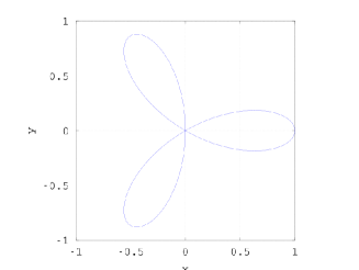
  Figure 1. Speed profile for planar solutions of the Novikov–Veselov equation

• The additive constant $k_{2}$ moves the KdV solution up or down in the graph.

• Replacing $s$ by $s+k_{1}\,t$ (with $k_{1}=\frac{3\,\beta}{4}-k_{2}\frac{3\,\kappa}{2}$) corresponds to observing the KdV solution in a moving frame, where the frame moves with velocity $-k_{1}$.

3. A Pseudo-Spectral method for the solution of (2+1) nonlinear wave equations

To numerically solve (1.1)–(1.3) we use a semi–implicit leap–frog spectral method based on the method in [7]. We restrict ourselves to a finite spatial domain $\Omega=[0,W_{x}]\times[0,W_{y}]$ with periodic boundary conditions. Thus we work on a torus topology and for the numerical results we have to observe the traveling waves across the boundary. We must also choose the domain large enough for the problem at hand.

This method uses the Fast Fourier Transform (FFT) to compute the spatial evolution and a leapfrog scheme to compute the time-stepping. The numerical scheme can be summarized as follows:

The Fourier transform of (1.1)–(1.3) is

$$4\,\hat{u}_{t} = i\,\left(\xi^{3}-3\,\xi\,\eta^{2}\right)\,\hat{u}+3\,i\,\xi\,\mathcal{F}[(uv)]+3\,i\,\eta\,\mathcal{F}[(uw)],$$ (3.1)

$$\xi\,\hat{u} = \xi\,\hat{v}-\eta\,\hat{w},$$ (3.2)

$$\eta\,\hat{u} = -\eta\,\hat{v}-\nu\,\hat{w}.$$ (3.3)

As usual, $\hat{u}$ refers to the Fourier transform $F$ of $u$ and is given by

$$\hat{u}_{p,q} = \mathcal{F}[u_{l,m}]=\sum_{l=0}^{L-1}\sum_{m=0}^{M-1}u_{l,m}\,e^{-i(\xi_{p}x_{l}+\eta_{q}y_{m})},$$

$$u_{l,m} = \mathcal{F}^{-1}[\hat{u}_{p,q}]=\frac{1}{L\,M}\,\sum_{p=-L/2}^{L/2-1}\sum_{q=-M/2}^{M/2-1}\hat{u}_{p,q}\,e^{i(\xi_{p}x_{l}+\eta_{q}y_{m})}.$$

The parameters $L$ and $M$ are the number of grid points in $[0,W_{x}]\times[0,W_{y}]$, respectively. They need to be powers of two in order to use the standard FFT. The spatial grid is defined by $(x_{l},y_{m})=(l\Delta x,m\Delta y)$ where $l=0,\ldots,L-1$, and $m=0,\ldots,M-1$. The spectral variables are $\left(\xi_{p},\eta_{q}\right)=\left(2\pi p/W_{x},2\pi q/W_{y}\right)$, with $p=-L/2,\ldots$, $-1,0,1,\ldots,L/2$, and $q=-M/2,\ldots$, $-1,0,1,\ldots,M/2$.

Equations (3.2) and (3.3) can be solved in terms of $\hat{u}$

$$\hat{v}=\frac{\xi^{2}-\eta^{2}}{\xi^{2}+\eta^{2}}\,\hat{u},\qquad\hat{w}=\frac{-2\eta\,\xi}{\eta^{2}+\xi^{2}}\,\hat{u}$$ (3.4)

Special attention has to be paid to the case $\xi^{2}+\eta^{2}=0$. The corresponding Fourier coefficient represent the average values of the functions $v$ and $w$.

Let ${\vec{c}}(t)$ be the vector with the $LM$ Fourier coefficients of the solution $u(x,y,t)$. Then solving (3.2), (3.3) and computing $-3\,i\,(\xi\,\mathcal{F}[(uv)]+\eta\,\mathcal{F}[(uw)])$ may be written as one nonlinear function $\vec{F}({\vec{c}})$. With the well constructed diagonal matrix $\mathbf{D}$ the NV equation (3.1) reads as

$$4\,\frac{d}{dt}\,{\vec{c}}(t)=\mathbf{D}\,{\vec{c}}(t)+\vec{F}({\vec{c}}(t))$$ (3.5)

For the time integration we use a symmetric three-level difference method for the linear terms, and a leapfrog method for the nonlinear terms. For the parameter $0\leq\theta\leq 1$ we use a superscript to refer to the time iteration and the above leads to

$$\frac{4}{2\,\Delta t}\,({\vec{c}}\,^{n+1}-{\vec{c}}\,^{n-1}) = \theta\,\mathbf{D}\,(\vec{c}\,^{n+1}+\vec{c}\,^{n-1})+(1-2\,\theta)\,\mathbf{D}\,\vec{c}\,^{n}+\vec{F}(\vec{c}\,^{n})$$

$$(2-\theta\,\Delta t\,\mathbf{D})\,\vec{c}\,^{n+1} = (1-2\,\theta)\,\Delta t\,\mathbf{D}\,\vec{c}\,^{n}+(2+\theta\,\Delta t\,\mathbf{D})\,\vec{c}\,^{n-1}$$

$$+\Delta t\,\vec{F}(\vec{c}\,^{n})$$

Thus we have an implicit scheme for the linear contribution and an explicit scheme for the nonlinear contribution. Since the matrix $\mathbf{D}$ is diagonal we do not have to solve a system of linear equations at each time step. For the special case $\theta=1/2$ we obtain a Crank Nicolson scheme

$$(4-\Delta t\,\mathbf{D})\,\vec{c}\,^{n+1}=+(4+\Delta t\,\mathbf{D})\,\vec{c}\,^{n-1}+2\,\Delta t\,\vec{F}(\vec{c}\,^{n})$$

For the three level method we need a separate method for the first time step. For the sake of simplicity we may choose $\vec{c}\,^{-1}=\vec{c}\,^{0}$. For computations with known solutions, e.g. (1.4), we use the known values of the solution at time $-\Delta t$.

3.1. Linear Numerical Stability Analysis

To gain insight into the stability of the spectral method, we include a linear stability analysis. The parameters determined here were used in the numerical experiments that follow. We examine the problem on a domain $\Omega=[0,W]\times[0,W]\subset{\mathbb{R}}^{2}$ and use periodic boundary conditions. Thus we examine the initial boundary value problem

$$\begin{array}[]{l}4\,u_{t}=-u_{xxx}+3\,u_{xyy}+3\,\alpha\,(v_{x}+w_{y}),\\ u_{x}=v_{x}-w_{y},\qquad u_{y}=-w_{x}-v_{y}\end{array}$$ (3.7)

The case $\alpha=0$ is the linearization of (1.1)–(1.3) about the zero solution. The utility of a linear stability analysis for a nonlinear system was addressed in [7] in the context of the KP and ZK equations, where they found that their results for the linear stability analysis were validated by numerical results and argued that while the analysis does not prove stability and convergence of the nonlinear scheme, the obtained stability conditions often suffice in practice. When implemented on a domain with periodic boundary condition (3.7) leads to

$$\begin{array}[]{ll}4\,u_{t}=-u_{xxx}+3\,u_{xyy}+3\,\alpha\,(v_{x}+w_{y}),&(x,y)\times t\in\Omega\times{\mathbb{R}},\\ u_{x}=v_{x}-w_{y},\qquad u_{y}=-w_{x}-v_{y}&\\ u(x,y,0)=u_{0}(x,y),&(x,y)\in\Omega,\\ u(x,y,t)=u(x+W_{x},y,t),&(x,y)\times t\in{\mathbb{R}}^{3},\\ u(x,y,t)=u(x,y+W_{y},t),&(x,y)\times t\in{\mathbb{R}}^{3},\end{array}$$ (3.8)

Using Fourier series and (3.4) this leads to

$$4\,\hat{u}_{t} = i\,(\xi^{3}-3\,\xi\,\eta^{2})\,\hat{u}+3\,i\,\xi\,\alpha\,\frac{\xi^{2}-\eta^{2}}{\eta^{2}+\xi^{2}}\,\hat{u}+3\,i\,\eta\,\alpha\,\frac{-2\eta\,\xi}{\eta^{2}+\xi^{2}}\,\hat{u}$$

$$= i\,\omega\,\hat{u}+i\,\frac{3\,\omega\,\alpha}{\eta^{2}+\xi^{2}}\,\hat{u}$$

where $\omega=\xi^{3}-\xi\,\eta^{2}$. This is an ODE of the form

$$4\,\frac{d}{dt}\,u(t)=i\,\lambda\,u(t)+i\,\gamma\,u(t)$$ (3.9)

where $\lambda=\omega=\xi^{3}-3\,\xi\,\eta^{2}$ and $\gamma=\omega\,\frac{3\,\alpha}{\eta^{2}+\xi^{2}}$. Using the numerical scheme (3) this leads to

$$(2-i\,\theta\,\lambda\,\Delta t)\,u^{n+1}=i\,(1-2\,\theta)\,\lambda\,\Delta t\,u^{n}+(2+i\,\theta\,\lambda\,\Delta t)\,u^{n-1}+i\,\gamma\,\Delta t\,u^{n}$$

or with

$$b_{1}=2+i\,\theta\,\lambda\,\Delta t\,\in{\mathbb{C}},\qquad b_{2}=i\,((1-2\,\theta)\,\lambda+\gamma)\,\Delta t\in{\mathbb{C}}$$ (3.10)

to the iteration matrix

$$\left(\begin{array}[]{c}u^{n+1}\\ u^{n}\end{array}\right)=\mathbf{M}\,\left(\begin{array}[]{c}u^{n}\\ u^{n-1}\end{array}\right)=\left[\begin{array}[]{*{2}{c}}\frac{b_{2}}{\overline{b_{1}}}&\frac{b_{1}}{\overline{b_{1}}}\\ 1&0\end{array}\right]\,\left(\begin{array}[]{c}u^{n}\\ u^{n-1}\end{array}\right)$$

For the system to be stable we have to verify that the norm of the eigenvalues $z_{1,2}$ of $\mathbf{M}$ are less or equal to 1. The characteristic equation is given by

$$\Phi_{NV}(z)=z^{2}-\frac{b_{2}}{\overline{b_{1}}}\,z-\frac{b_{1}}{\overline{b_{1}}}=0$$

Thus we conclude $|z_{i}\cdot z_{2}|=|\frac{b_{1}}{\overline{b_{1}}}|=1$ and stability of the solution is equivalent to $|z_{1,2}|=1$ , i.e. we have $|u^{n+1}|=|u^{n-1}|$. Using the explicit solution for quadratic equations and

$$b_{2}\in i\,{\mathbb{R}},\qquad|b_{2}|\leq 2\,|b_{1}|$$ (3.11)

we find

$$2\,\overline{b_{1}}\,z_{1,2} = b_{2}\pm\sqrt{b_{2}^{2}+4\,\overline{b_{1}}\,b_{1}}\,=\,b_{2}\pm\sqrt{b_{2}^{2}+4\,|b_{1}|^{2}}$$

$$|2\,\overline{b_{1}}|^{2}\,|z_{1,2}|^{2} = |b_{2}|^{2}-|b_{2}|^{2}+4\,|b_{1}|^{2}\,=\,|2\,b_{1}|^{2}$$

and consequently $|z_{1,2}|=1$ . With (3.10) the stability condition (3.11) for the ODE (3.9) is

$$((1-2\,\theta)\,\lambda+\gamma)^{2}\,(\Delta t)^{2} \leq 4\,|2+i\,\theta\,\lambda\,\Delta t\,|^{2}$$

$$\left(((1-2\,\theta)\,\lambda+\gamma)^{2}-(2\,\theta\,\lambda)^{2}\right)\,(\Delta t)^{2} \leq 16$$

$$((1-4\,\theta)\,\lambda^{2}+2\,(1-2\,\theta)\,\lambda\,\gamma+\gamma^{2})\,(\Delta t)^{2} \leq 16$$

For $\gamma=\alpha=0$ and $\frac{1}{4}\leq\theta\leq 1$ the stability condition is satisfied, independent on the step size $0<\Delta t$ and we have a stability result for the initial boundary value problem (3.8) .

Theorem 1.

Apply the numerical scheme (3) to the linearization of (1.1)–(1.3) about the zero solution, i.e. to the equation

$$\begin{array}[]{rcl}4\,u_{t}&=&-u_{xxx}+3\,u_{xyy}\\ u_{x}&=&v_{x}-w_{y}\;,\qquad u_{y}=-w_{x}-v_{y}\end{array}$$

This scheme is stable for $\frac{1}{4}\leq\theta\leq 1$.

Proving stability for (3.8) with $\alpha\neq 0$ requires a few more computations. Use the expressions for $\lambda=\omega=\xi^{3}-3\,\xi\,\eta^{2}$ and $\gamma=\omega\,\frac{3\,\alpha}{\eta^{2}+\xi^{2}}$ in (3.9) and the stability condition reads as

$$((1-4\,\theta)\,\lambda^{2}+2\,(1-2\,\theta)\,\lambda\,\gamma+\gamma^{2})\,(\Delta t)^{2} \leq 16$$

$$\omega^{2}\;((1-4\,\theta)\,+2\,(1-2\,\theta)\,\frac{3\,\alpha}{\eta^{2}+\xi^{2}}+\frac{9\,\alpha^{2}}{(\eta^{2}+\xi^{2})^{2}})\,(\Delta t)^{2} \leq 16$$

$$(1-4\,\theta)\,+2\,(1-2\,\theta)\,\frac{3\,\alpha}{\eta^{2}+\xi^{2}}+\left(\frac{3\,\alpha}{\eta^{2}+\xi^{2}}\right)^{2} \leq \left(\frac{4}{\omega\,\Delta t}\right)^{2}$$

For $\theta=\frac{1}{2}$ we find the sufficient conditions.

$$-2+\left(\frac{3\,\alpha}{\eta^{2}+\xi^{2}}\right)^{2}\,\leq\,\left(\frac{3\,\alpha}{\eta^{2}+\xi^{2}}\right)^{2} \leq \left(\frac{4}{(\xi^{3}-3\,\xi\,\eta^{2})\,\Delta t}\right)^{2}$$

$$(\Delta t)^{2} \leq \left(\frac{4\,(\xi^{2}+\eta^{2})}{3\,\alpha\,(\xi^{3}-3\,\xi\,\eta^{2})}\right)^{2}$$

Since $|\xi^{3}-3\,\xi\,\eta^{2}|\leq(\xi^{2}+\eta^{2})\cdot\max\{|\xi|,\,|\eta|\}$ we have the sufficient condition

$$\Delta t\leq\frac{4}{3\,|\alpha|\,\max\{|\xi|,\,|\eta|\}}$$ (3.12)

For the DFT with $\Delta x=\Delta y=\frac{W_{x}}{L}$ we find $\max\{|\xi|,\,|\eta|\}=\frac{\pi}{\Delta x}$ and thus we have the stability condition

$$\Delta t\leq\frac{4}{3\,|\alpha|\,\pi}\;\Delta x$$ (3.13)

As a consequence we have a stability result for the initial boundary value problem (3.8) with $\alpha\neq 0$.

Theorem 2.

Apply the numerical scheme (3) to (3.8), i.e.

$$\begin{array}[]{rcl}4\,u_{t}&=&-u_{xxx}+3\,u_{xyy}+3\,\alpha\,(v_{x}+w_{y})\\ u_{x}&=&v_{x}-w_{y}\;,\qquad u_{y}=-w_{x}-v_{y}\end{array}$$

This scheme is stable for $\theta=\frac{1}{2}$ if the time step $\Delta t$ satisfies condition (3.13).

4. Instability of traveling-wave solutions of the NV-equation to transverse perturbations

The   K-expansion method presented by Allen and Rowlands considers long wavelength perturbations in the transversal direction. It was originally used to investigate the stability of solutions to the Zakharov–Kuznetsov equation, a non-integrable generalization of the KdV equation [10, 11, 9]. Since then the method has been applied to the KP equation and the modified ZK (mZK) equation [18]. This is the second application of the method to a system of PDE’s, the first being by Bradley [5].

4.1. The modified equations

To begin, we transform the system to move along with the soliton by using new independent and dependent variables. Using

$$(t,x,y)\mapsto\sqrt{c}\,(\alpha\,t,x-c\,t,y)=(\tilde{t},\tilde{x},\tilde{y})$$

and

$$(u,v_{1},v_{2})\mapsto c\,(u,v_{1},v_{2})$$

or

$$u(t,x,y) = c\;\tilde{u}(t\,c^{3/2},(x-c\,t)\,c^{1/2},y\,c^{1/2})$$

$$v_{1}(t,x,y) = c\;\tilde{v}_{1}(t\,c^{3/2},(x-c\,t)\,c^{1/2},y\,c^{1/2})$$ (4.1)

$$v_{2}(t,x,y) = c\;\tilde{v}_{2}(t\,c^{3/2},(x-c\,t)\,c^{1/2},y\,c^{1/2}),$$

the NV equations (1.1)–(1.3) are transformed to

$$0 = 4u_{t}-4u_{x}+u_{xxx}-3u_{xyy}-3(uv)_{x}-3(uw)_{y},$$ (4.2)

$$u_{x} = +v_{x}-w_{y},$$ (4.3)

$$u_{y} = -w_{x}-v_{y}$$ (4.4)

For sake of a more readable notation we dropped the tildes on the new dependent and independent variables. The known solution

$$f_{c}(x-c\,t)=-2\,c\,\mathop{\rm sech}\nolimits^{2}(\sqrt{c}\,(x-c\,t))$$

of the original system turns into a stationary solution of the modified system.

$$u_{0}(x)=v_{0}(x)=-2\,\mathop{\rm sech}\nolimits^{2}(x),\qquad w_{0}(x)=0$$

Now we examine perturbed functions of the form

$$u(x,y,t) = u_{0}(x)+\epsilon\,f(x)\,e^{iky+\gamma t},$$ (4.5)

$$v(x,y,t) = v_{0}(x)+\epsilon\,g(x)\,e^{iky+\gamma t},$$ (4.6)

$$w(x,y,t) = w_{0}(x)+\epsilon\,h(x)\,e^{iky+\gamma t}.$$ (4.7)

Thus we examine periodic, transversal perturbations with exponential growth. For numerical purposes we may also work with a purely real formulation.

$$u(x,y,t) = u_{0}(x)+\epsilon\,f(x)\,\cos(k\,y)\,e^{\gamma t},$$ (4.8)

$$v(x,y,t) = v_{0}(x)+\epsilon\,g(x)\,\cos(k\,y)\,e^{\gamma t},$$ (4.9)

$$w(x,y,t) = w_{0}(x)+\epsilon\,h(x)\,\sin(k\,y)\,e^{\gamma t}.$$ (4.10)

Substituting these expressions into (4.2)–(4.4) and dropping terms propotional to $\epsilon^{2}$ leads to (use ^′ for $\frac{d}{dx}$)

$$0 = 4\,\gamma\,f-4\,f^{\prime}+f^{{\prime}{\prime}{\prime}}+3\,k^{2}\,f^{\prime}$$ (4.11)

$$-3\,(u_{0}\,g)^{\prime}-3\,(v_{0}\,f)^{\prime}-3\,u_{0}\,i\,k\,h$$

$$f^{\prime} = +g^{\prime}-i\,k\,h$$ (4.12)

$$i\,k\,f = -h^{\prime}-i\,k\,g$$ (4.13)

This is a system of linear ordinary differential equations with non-constant coefficients. Use $h(x)=\frac{1}{i\,k}\,(g^{\prime}(x)-f^{\prime}(x))$ and the above can be written in the form

$$f^{{\prime}{\prime}{\prime}}(x) = (-4\,\gamma+3\,u_{0}^{\prime}(x))\,f(x)+(4-3\,k^{2})\,f^{\prime}(x)+$$ (4.14)

$$+3\,u_{0}^{\prime}(x)\,g(x)+6\,u_{0}(x)\,g^{\prime}(x)$$

$$g^{{\prime}{\prime}}(x) = k^{2}\,g(x)+f^{{\prime}{\prime}}(x)+k^{2}\,f(x)$$ (4.15)

4.2. Known solutions

Since the $f_{c}(x-c\,t+s)$ is a solution of the original NV equation  (1.1)–(1.3), we conclude that $(u_{0}(x-s),\,v_{0}(x-s),\,w_{0}(x-s))$ solve the system (4.2)–(4.4) and thus their derivatives must solve the linearized problem (4.11)–(4.13). Since $\frac{d}{dx}\,\mathop{\rm sech}\nolimits^{2}(x)=-2\,\mathop{\rm sech}\nolimits^{2}(x)\,\tanh(x)$ we find solutions

$$f(x)=g(x)=\mathop{\rm sech}\nolimits^{2}(x)\,\tanh(x)\;,\qquad h(x)=0$$ (4.16)

for $k=\gamma=0$ to the system (4.14)–(4.15). For $k=1$ and $\gamma=0$ we found

$$f(x) = +\mathop{\rm sech}\nolimits^{3}(x)$$

$$g(x) = -\mathop{\rm sech}\nolimits(x)\,\tanh^{2}(x)$$ (4.17)

$$h(x) = -i\,\mathop{\rm sech}\nolimits(x)\,\tanh(x)$$

as a second, explicit solution of (4.11)–(4.13).

With the help of these solutions we will construct unstable solution to the Novikov-Veselov equations, as function of the parameters $k$ and $\gamma$. Thus we need nonzero solutions of (4.14)–(4.15).

4.3. Locating unstable solutions

Using the function $u_{0}(x)=-2\,\mathop{\rm sech}\nolimits^{2}(x)$, a matrix notation translates the high order system (4.14)–(4.15) into a system of first order ordinary differential equations.

$$\frac{d}{dx}\;\left(\begin{array}[]{c}f\\ f^{\prime}\\ f^{{\prime}{\prime}}\\ g\\ g^{\prime}\end{array}\right)\,=\,\left[\begin{array}[]{*{5}{c}}0&1&0&0&0\\ 0&0&1&0&0\\ -4\,\gamma+3\,u_{0}^{\prime}&(4-3\,k^{2})&0&3\,u_{0}^{\prime}(x)&6\,u_{0}\\ 0&0&0&0&1\\ k^{2}&0&1&k^{2}&0\end{array}\right]\;\left(\begin{array}[]{c}f\\ f^{\prime}\\ f^{{\prime}{\prime}}\\ g\\ g^{\prime}\end{array}\right)$$

4.3.1. Behavior of solution for large $|x|$

For large values of $|x|$ we use $u_{0}(x)\approx 0$ and arrive at a decoupled system of linear differential equations with constant coefficients.

$$\frac{d}{dx}\;\left(\begin{array}[]{c}f\\ f^{\prime}\\ f^{{\prime}{\prime}}\end{array}\right) = \left[\begin{array}[]{*{3}{c}}0&1&0\\ 0&0&1\\ -4\,\gamma&(4-3\,k^{2})&0\\ \end{array}\right]\;\left(\begin{array}[]{c}f\\ f^{\prime}\\ f^{{\prime}{\prime}}\end{array}\right)$$ (4.27)

$$\frac{d}{dx}\;\left(\begin{array}[]{c}g\\ g^{\prime}\end{array}\right) = \left[\begin{array}[]{*{2}{c}}0&1\\ k^{2}&0\end{array}\right]\;\left(\begin{array}[]{c}g\\ g^{\prime}\end{array}\right)+\left(\begin{array}[]{c}0\\ k^{2}\,f^{\prime}+f^{{\prime}{\prime}}\end{array}\right)$$ (4.36)

The characteristic equation of the matrix in (4.27) is given by

$$\lambda^{3}+(3\,k^{2}-4)\,\lambda+4\,\gamma=0,$$ (4.37)

and we will denote the eigenvalues $\lambda_{1},\lambda_{2}$, and $\lambda_{3}$ of this system by $p_{1},p_{2}$, and $p_{3}$, respectively. The inhomogeneous system in (4.36) leads to eigenvalues $\lambda_{4,5}=\pm k$. Using Cardano’s formulas for zeros of polynomials of degree 3, we verify that (4.37) has three distinct real values if

$$4\,\gamma^{2}+\frac{(3\,k^{2}-4)^{3}}{27}<0.$$

For our domain of $(k,\gamma)$ to be examined we may use

$$p_{3}\leq 0\leq p_{1},\,p_{2}$$

and for small values of $|\gamma|$ we find

$$\lambda(\gamma)=\left\{\begin{array}[]{ll}p_{1}\,\approx\,0+\frac{4}{4-3\,k^{2}}\,\gamma&\\ p_{2}\,\approx\,+\sqrt{4-3\,k^{2}}-\frac{2}{4-3\,k^{2}}\,\gamma&\\ p_{3}\,\approx\,-\sqrt{4-3\,k^{2}}-\frac{2}{4-3\,k^{2}}\,\gamma&\end{array}\right.$$ (4.38)

with the solution of the form $f(x)\approx c_{1}e^{p_{1}x}+c_{2}e^{p_{2}x}+c_{3}e^{p_{3}x}$. We examine $\gamma\geq 0$, and for $x\to+\infty$ we require the solution $f(x)$ of (4.27) to be bounded, and thus

$$f(x)\approx f_{+}(x)=c_{3}\,e^{p_{3}\,x}.$$

Next, examine (4.36) in the form

$$g_{+}^{{\prime}{\prime}}(x)-k^{2}\,g_{+}(x)=k^{2}\,f_{+}(x)+f_{+}^{{\prime}{\prime}}(x)=c_{3}\,(k^{2}+p_{3}^{2})\,e^{p_{3}\,x}$$

with the solution

$$g_{+}(x)=\beta_{1}\,e^{+k\,x}+\beta_{2}\,e^{-k\,x}+c_{3}\,\frac{k^{2}+p_{3}^{2}}{p_{3}^{2}-k^{2}}\,e^{p_{3}\,x}.$$

Since this solution has to remain bounded as $x\to+\infty$, we find

$$g_{+}(x)=\beta_{2}\,e^{-k\,x}+c_{3}\,\frac{k^{2}+p_{3}^{2}}{p_{3}^{2}-k^{2}}\,e^{p_{3}\,x}.$$

The case $\gamma\geq 0$ and $x\to-\infty$, leads in an analogous way to

$$f(x)\approx f_{-}(x)=c_{1}\,e^{p_{1}\,x}+c_{2}\,e^{p_{2}\,x}$$

and

$$g(x)\approx g_{-}(x)=\beta_{1}\,e^{+k\,x}+c_{1}\,\frac{k^{2}+p_{1}^{2}}{p_{1}^{2}-k^{2}}\,e^{p_{1}\,x}+c_{2}\,\frac{k^{2}+p_{2}^{2}}{p_{2}^{2}-k^{2}}\,e^{p_{2}\,x}.$$

For $0<k^{2}\ll 1$ we find

$$p_{1}^{2}\approx\frac{4^{2}}{(4-3\,k^{2})^{2}}\,\gamma^{2}\approx\gamma^{2}$$ (4.39)

and thus the above formula for $g_{(}x)$ may not be valid for $\gamma^{2}\approx k^{2}\ll 1$ . For $k=0$ the equation for $g$ simplifies to $g^{{\prime}{\prime}}(x)=f^{{\prime}{\prime}}(x)$, and the conditions at $x=\pm\infty$ imply $g(x)=f(x)$.

4.3.2. Solutions for intermediate $|x|$.

Choosing a large value for $M>0$, we construct nontrivial solutions to (4.14)–(4.15) for $-\infty<x\leq-M$, then for $-M\leq x\leq+M$, and then for $+M\leq x<+\infty$. We seek nonzero values of the parameters $(c_{1},\,c_{2},\,c_{3},\,\beta_{1},\,\beta_{2})$, such that we find a nonzero solution.

Use the solutions $f_{-}$ and $g_{-}$ to define a matrix

$$\mathbf{T}_{-}=\left[\begin{array}[]{*{5}{c}}e^{-p_{1}\,M}&e^{-p_{2}\,M}&0&0&0\\ p_{1}\,e^{-p_{1}\,M}&p_{2}\,e^{-p_{2}\,M}&0&0&0\\ p_{1}^{2}\,e^{-p_{1}\,M}&p_{2}^{2}\,e^{-p_{2}\,M}&0&0&0\\ \frac{p_{1}^{2}+k^{2}}{p_{1}^{2}-k^{2}}\,e^{-p_{1}\,M}&\frac{p_{2}^{2}+k^{2}}{p_{2}^{2}-k^{2}}\,e^{-p_{2}\,M}&0&e^{-k\,M}&0\\ \frac{(p_{1}^{2}+k^{2})\,p_{1}}{p_{1}^{2}-k^{2}}\,e^{-p_{1}\,M}&\frac{(p_{2}^{2}+k^{2})\,p_{2}}{p_{2}^{2}-k^{2}}\,e^{-p_{2}\,M}&0&k\,e^{-k\,M}&0\end{array}\right]$$

with

$$\mathbf{T}_{-}\left(\begin{array}[]{c}c_{1}\\ c_{2}\\ c_{3}\\ \beta_{1}\\ \beta_{2}\end{array}\right)=\left(\begin{array}[]{c}f(-M)\\ f^{\prime}(-M)\\ f^{{\prime}{\prime}}(-M)\\ g(-M)\\ g^{\prime}(-M)\end{array}\right)$$

Use the solutions $f_{+}$ and $g_{+}$ to define a matrix

$$\mathbf{T}_{+}=\left[\begin{array}[]{*{5}{c}}0&0&e^{p_{3}\,M}&0&0\\ 0&0&p_{3}\,e^{p_{3}\,M}&0&0\\ 0&0&p_{3}^{2}\,e^{p_{3}\,M}&0&0\\ 0&0&\frac{p_{3}^{2}+k^{2}}{p_{3}^{2}-k^{2}}\,e^{p_{3}\,M}&0&e^{-k\,M}\\ 0&0&\frac{(p_{3}^{2}+k^{2})\,p_{3}}{p_{3}^{2}-k^{2}}\,e^{p_{3}\,M}&0&-k\,e^{-k\,M}\end{array}\right]$$

with

$$\mathbf{T}_{+}\left(\begin{array}[]{c}c_{1}\\ c_{2}\\ c_{3}\\ \beta_{1}\\ \beta_{2}\end{array}\right)=\left(\begin{array}[]{c}f(+M)\\ f^{\prime}(+M)\\ f^{{\prime}{\prime}}(+M)\\ g(+M)\\ g^{\prime}(+M)\end{array}\right)$$

Then use an ODE solver to examine the system (4.14)–(4.15) on the interval $[-M,M]$ as an initial value problem. This leads to a matrix $\mathbf{T}$ such that

$$\mathbf{T}\left(\begin{array}[]{c}f(-M)\\ f^{\prime}(-M)\\ f^{{\prime}{\prime}}(-M)\\ g(-M)\\ g^{\prime}(-M)\end{array}\right)=\left(\begin{array}[]{c}f(+M)\\ f^{\prime}(+M)\\ f^{{\prime}{\prime}}(+M)\\ g(+M)\\ g^{\prime}(+M)\end{array}\right)$$

Now we have two methods to compute the values of the solution at $x=+M$, and the system (4.14)–(4.15) has a nonzero solution if and only if

$$D(k,\gamma)\,=\,\det(\mathbf{M}(k,\gamma))=\det(\mathbf{T}\cdot\mathbf{T}_{-}-\mathbf{T}_{+})=0$$ (4.40)

Thus we examine solutions of this equation as functions of the parameters $k$ and $\gamma$.

4.4. The special case $k=0$

For $k=0$, equation (4.15) reads as $g^{{\prime}{\prime}}(x)=f^{{\prime}{\prime}}(x)$ and the only solution satisfying $g(\pm\infty)=f(\pm\infty)$ is $g(x)=f(x)$. Then (4.14) leads to

$$\frac{d}{dx}\,\left(\begin{array}[]{c}f\\ f^{\prime}\\ f^{{\prime}{\prime}}\end{array}\right)=\left[\begin{array}[]{*{3}{c}}0&1&0\\ 0&0&1\\ -4\,\gamma+6\,u_{0}^{\prime}&4+6\,u_{0}&0\end{array}\right]\;\left(\begin{array}[]{c}f\\ f^{\prime}\\ f^{{\prime}{\prime}}\end{array}\right)$$ (4.41)

Using the same approach as in the previous section we define

$$\mathbf{T}_{-}\,\left(\begin{array}[]{c}c_{1}\\ c_{2}\\ c_{3}\end{array}\right)=\left(\begin{array}[]{c}f(-M)\\ f^{\prime}(-M)\\ f^{{\prime}{\prime}}(-M)\end{array}\right) = \left[\begin{array}[]{*{3}{c}}e^{-p_{1}\,M}&e^{-p_{2}\,M}&0\\ p_{1}\,e^{-p_{1}\,M}&p_{2}\,e^{-p_{2}\,M}&0\\ p_{1}^{2}\,e^{-p_{1}\,M}&p_{2}^{2}\,e^{-p_{2}\,M}&0\end{array}\right]\,\left(\begin{array}[]{c}c_{1}\\ c_{2}\\ c_{3}\end{array}\right)$$

$$\mathbf{T}_{+}\,\left(\begin{array}[]{c}c_{1}\\ c_{2}\\ c_{3}\end{array}\right)=\left(\begin{array}[]{c}f(+M)\\ f^{\prime}(+M)\\ f^{{\prime}{\prime}}(+M)\end{array}\right) = \left[\begin{array}[]{*{3}{c}}0&0&e^{p_{3}\,M}\\ 0&0&p_{3}\,e^{p_{3}\,M}\\ 0&0&p_{3}^{2}\,e^{p_{3}\,M}\end{array}\right]\,\left(\begin{array}[]{c}c_{1}\\ c_{2}\\ c_{3}\end{array}\right)$$

$$\mathbf{T}_{0}\left(\begin{array}[]{c}f(-M)\\ f^{\prime}(-M)\\ f^{{\prime}{\prime}}(-M)\end{array}\right) = \left(\begin{array}[]{c}f(+M)\\ f^{\prime}(+M)\\ f^{{\prime}{\prime}}(+M)\end{array}\right)$$

where $\mathbf{T}_{0}$ is constructed using an ODE solver for (4.41). Then the system (4.14)–(4.15) has a nonzero solution for $k=0$ if and only if

$$D_{0}(\gamma)\,=\,\det(\mathbf{M}_{0}(\gamma))=\det(\mathbf{T}_{0}\cdot\mathbf{T}_{-}-\mathbf{T}_{+})=0$$ (4.45)

5. Numerical Results on the Instabilities of Plane-Wave Soliton Solutions

5.1. Locating unstable solutions

Based on expression (4.40) we generate plots of the function $D(k,\gamma)=\det(\mathbf{M}(k,\gamma))$ on a domain $0\leq k\leq 1$ and $0\leq\gamma\leq 0.5$, leading to Figure 2. In the corner $k\approx 1$ and $\gamma\approx 0.5$ the real part of the function vanishes, but a second plot verifies that the imaginary part is different from zero. Thus Figure 2 indicates that we have a clearly defined solution curve of $\det(\mathbf{M}(k,\gamma))=0$, away from the origin.

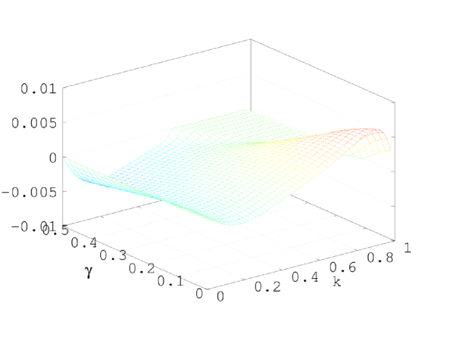
Figure 2. The real part of $\det(\mathbf{M})$ as a function of $k$ and $\gamma$

Since the behavior close to $(k,\gamma)\approx(0,\,0)$ is critical, we examine this section with a finer resolution, leading to Figure 3(a). The obvious spikes are caused by the zeros in the denominator in condition (4.39). Figure 3(a) suggests the existence of a solution along the axis $k=0$. Using (4.45) we generate Figure 3(b). As a consequence the only solution along the axis $k=0$ is at $\gamma=0$ . Thus the known solution (4.16) is an isolated solution in the parameter space $(k,\gamma)$ at $(0,\,0)$.

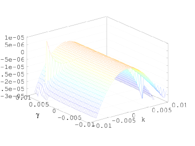
(a) $\det\,\mathbf{M}(k,\gamma)$ close to origin

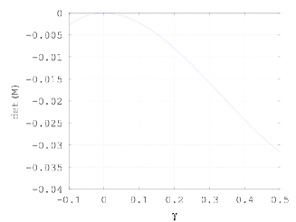
(b) $\det\,\mathbf{M}_{0}(\gamma)$

Figure 3. Behavior at the origin and along the axis $k=0$

With the above preparation we can now construct values of $(k,\gamma)$ leading to nonzero solutions of (4.14)–(4.15) and thus for $\gamma>0$ to unstable soliton solutions of the NV equations (1.1)–(1.3).

We trace a solution curve of (4.40) by generating an arc length parametrization of the curve. Using an arbitrary initial point on the curve (use a contour plot of Figure 2) and a starting direction, we minimize $|\det(\mathbf{M}(k,\gamma))|$ along a straight line segment orthogonal to the stepping direction. Using this local minimum, we adjust the stepping direction and then make a small step to follow the solution curve. While stepping along the curve we verify that we actually have a solution of (4.40), and not only a minimum. This proved to be a stable algorithm and generated Figure 4.

Observe that Figure 4(a) also displays negative values of $\gamma$, which do not lead to unstable solutions of (1.1)–(1.3). We display these values to confirm that we have a closed curve without branching points.

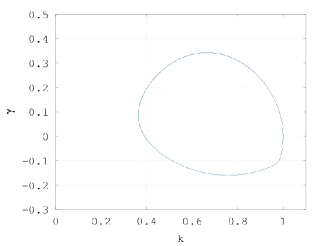
(a) solution curve of $|\det(\mathbf{M})|=0$

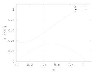
(b) parameters leading to unstable solutions

Figure 4. Solution curve of $|\det(\mathbf{M})|=0$ and parameters $k$ and $\gamma$ leading to unstable solutions

For the parameter values of $(k,\gamma)$ in Figure 4(b) there are nonzero functions $f(x)$, $g(x)$ and $h(x)$, such that for small $\epsilon$ we have solutions of the equations (4.2)–(4.4) of the form (4.5)–(4.7). Since the $y$ dependence of these functions is of the form $e^{i\,k\,y}$, the functions are periodic in $y$ with a period of $L_{y}=\frac{2\,\pi}{k}$. The corresponding exponent is shown in Figure (4(b)). Thus the Novikov–Veselov equations (1.1)–(1.3) with initial condition $u(x,y,0)=-2\,c\,\mathop{\rm sech}\nolimits^{2}(\sqrt{c}\,x)$ will lead to an unstable soliton solution.

Theorem 3.

The soliton solutions $u(x,y,t)=v(x,y,t)=-2\,c\,\mathop{\rm sech}\nolimits^{2}(\sqrt{c}\,(x-c\,t))$ and $w(x,y,t)=0$ of the NV equations (1.1)–(1.3) are not stable. For values of $0.363<k\leq 1$ there are $y$–periodic, unstable contributions with a period of $L_{y}=\frac{2\,\pi}{k\,\sqrt{c}}$.

5.2. Constructing unstable solutions numerically

As an example, in this section we construct one of the above unstable solutions numerically, using the algorithm from Section 3 for periodic solutions in $x$ and $y$. Since the soliton solution $\mathop{\rm sech}\nolimits^{2}(x)$ decays rapidly, the above results still apply when working on a sufficiently large domain. The steps of the algorithm are as follows:

1. Choose values of $(k,\gamma)$ in Figure 4(b) and determine the eigenvector $(c_{1},c_{2},c_{3},\beta_{1},\beta_{2})$ for the zero eigenvalue.

2. Use the algorithm leading to the matrices $\mathbf{T}$, $\mathbf{T}_{-}$ and $\mathbf{T}_{+}$ to construct the nonzero functions $f(x),g(x),h(x)$.

3. Pick a size domain such that $\frac{2\,\pi}{k}$ periodic functions in $y$ are admissable.

4. Construct initial values, using (4.8)–(4.10), use a small value of $\epsilon$. Without taking the transformations (4.1) into account we obtain a speed of $c=1$ of the unperturbed soliton.

5. Solve the NV equations  (1.1)–(1.3), using the algorithm presented in Section 3.

6. The deviation from the single soliton solution should not change its shape, but the size is expected to be proportional to $e^{\gamma\,t}$.

7. Solitions for speeds $c\neq 1$ can be constructed similarly, using the transformations (4.1).

The evolution of a perturbed soliton from Theorem 3 was computed using the semi-implicit pseudo-spectal method. Here we chose $k=0.504$ and $\gamma=0.296$, and the graph of the perturbation $f(x)$ is found in Figure 6(a). As initial value we chose a perturbed KdV solition with speed $c=1$, starting at $x=10$. Find the solution and the difference to the unperturbed KdV soliton at time $5$ in Figure 5. The corresponding animations are available on the web site [22]. The exponential growth of the perturbation with exponent $\gamma$ is numerically confirmed.

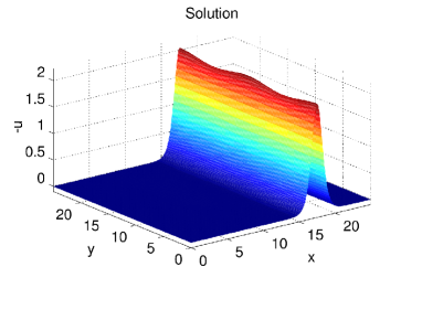
(a) shape of the solution

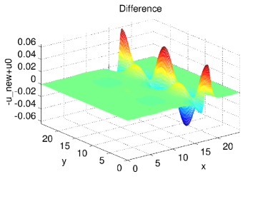
(b) shape of the perturbation

Figure 5. A perturbed solution at time 5

One can construct the shapes of the functions $f(x)$ for all positive values of $\gamma$ along the arc in Figure 4 to obtain Figure 6(b). The solutions constructed for $(k,\gamma)=(1,\,0)$ have to match the known exact solutions (4.17), which is confirmed.

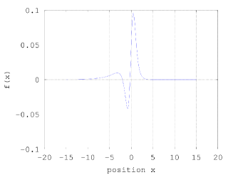
(a) at $k\approx 0.5$ and $\gamma\approx 0.3$

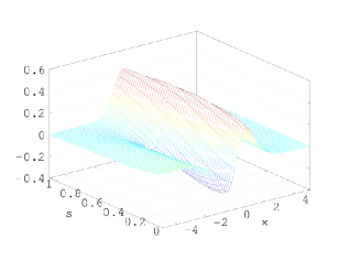
(b) as function of arc length $s$

Figure 6. Shape of the perturbations $f(x)$

6. Conclusions

In this work a semi-implicit pseudo-spectral method was introduced for the numerical computation of evolutions of solutions to the NV equation, constituting the first numerical implementation of a spectral method for a system of soliton nonlinear PDE’s. A linear stability analysis yields a stability condition for the Crank-Nicolson scheme on the linearized IBVP. The instability of traveling wave solutions to transverse perturbations was established by the K-expansion method, and unstable soliton solutions were constructed. The evolution of an example was computed numerically by the semi-implicit pseudo-spectral method.

References

- [1] M. A. Allen and Phibanchon, Time evolution of perturbed solitons of modified Kadomtsev-Petviashvili equations, Computational Science and its Applications, 2007. ICCSA 2007. International Conference on (2007), 20–23.
- [2] M. A. Allen and G. Rowlands, Determination of the growth rate for the linearized Zakharov-Kuznetsov equation, Journal of Plasma Physics 50 (1993), no. 03, 413–424.
- [3] by same author, On the transverse instabilities of solitary waves, Physics Letters A 235 (1997), 145–146.
- [4] L. V. Bogdanov, The Veselov-Novikov equation as a natural generalization of the Korteweg-de Vries equation, Teoret. Mat. Fiz. 70 (1987), no. 2, 309–314. MR MR894472 (88k:35170)
- [5] R. Mark Bradley, Electromigration-induced soliton propagation on metal surfaces, Phys. Rev. E 60 (1999), no. 4, 3736–3740.
- [6] T. J. Bridges, Transverse instability of solitary-wave states of the water-wave problem, Journal of Fluid Mechanics 439 (2001), 255–278.
- [7] B. F. Feng, T. Kawahara, and T. Mitsui, A conservative spectral method for several two-dimensional nonlinear wave equations, Journal of Computational Physics 153 (1999), no. 2, 467 – 487.
- [8] P. Frycz and E. Infeld, Self-focusing of nonlinear ion-acoustic waves and solitons in magnetized plasmas. part 3. Arbitrary-angle perturbations, period doubling of waves, J. Plasma Phys. 41 (1989), 441–446.
- [9] P. Frycz and E. Infeld, Self-focusing of nonlinear ion-acoustic waves and solitons in magnetized plasmas. part 3. Arbitrary-angle perturbations, period doubling of waves, J. Plasma Phys. 41 (1989), no. 03, 441–446.
- [10] E. Infeld, Self-focusing of nonlinear ion-acoustic waves and solitons in magnetized plasmas, J. Plasma Phys. 33 (1985), no. 02, 171–182.
- [11] E. Infeld and P. Frycz, Self-focusing of nonlinear ion-acoustic waves and solitons in magnetized plasmas. part 2. Numerical simulations, two-soliton collisions, J. Plasma Phys. 37 (1987), no. 01, 97–106.
- [12] Eryk Infeld and George Rowlands, Nonlinear waves, solitons and chaos, second ed., Cambridge University Press, Cambridge, 2000. MR 1780300 (2001f:76019)
- [13] Rowlands G. Infeld E. and Senatorski A., Instabilities and oscillations of one and two dimensional Kadomtsev -Petviashvili waves and solitons, Proc R Soc A 455 (1999), 4363–4381.
- [14] B.B. Kadomtsev and V.I. Petviashvili, On the stability of solitary waves in weakly dispersing media, Soviet Physics Doklady 15 (1970), 539–+.
- [15] M. Lassas, J. L Mueller, and S. Siltanen, Mapping properties of the nonlinear Fourier transform in dimension two, Communications in Partial Differential Equations 32 (2005), no. 4, 591–610.
- [16] M. Lassas, J. L Mueller, S. Siltanen, and A. Stahel, The Novikov-Veselov Equation and the Inverse Scattering Method, Part I: Analysis, Physica D 241 (2012), no. 16, 1322–1335.
- [17] by same author, The Novikov-Veselov Equation and the Inverse Scattering Method, Part II: Computation, Nonlinearity 24 (2012), 1799–1818.
- [18] S. Munro and E. J. Parkes, The derivation of a modified Zakharov-Kuznetsov equation and the stability of its solutions, J. Plasma Phys. 62 (1999), no. 03, 305–317.
- [19] M Music, P Perry, and S Siltanen, Exceptional circles of radial potentials, Inverse Problems 29 (2013), 045004.
- [20] Veselov A P and Novikov S P, Finite-zone, two-dimensional, potential schrödinger operators. Explicit formulas and evolution equations, Sov. Math. Dokl 30 (1984), 558–591.
- [21] P. A. Perry, Miura maps and inverse scattering for the Novikov-Veselov equation, Preprint (arXiv:1201.2385v1 11 Jan 2012) (2012).
- [22] A. Stahel, staff.ti.bfh.ch/sha1/NovikovVeselov/NovikovVeselov.html.
- [23] Li-Yeng Sung, An inverse scattering transform for the Davey-Stewartson II equations. I,II,III, J. Math. Anal. Appl. 183 (1994), 121–154, 289–325, 477–494.