On the origin of the radio emission of Sw 1644+57

Abstract

We apply relativistic equipartition synchrotron arguments to the puzzling radio emission of the tidal disruption event candidate Sw 1644+57. We find that, regardless of the details of the equipartition scenario considered, the energy required to produce the observed radio (i.e., energy in the magnetic field and radio emitting electrons) must increase by a factor of $\sim 20$ during the first 200 days. It then saturates. This energy increase cannot be alleviated by a varying geometry of the system. The radio data can be explained by: (i) An afterglow like emission of the X-ray emitting narrow relativistic jet. The additional energy can arise here from a slower moving material ejected in the first few days that gradually catches up with the slowing down blast wave (Berger et al. 2012). However, this requires at least $\sim 4\times 10^{53}$ erg in the slower moving outflow. This is much more than the energy of the fast moving outflow that produced the early X-rays and it severely constrains the overall energy budget. (ii) Alternatively, the radio may arise from a mildly relativistic and quasi-spherical outflow. Here, the energy available for radio emission increases with time reaching at least $\sim 10^{51}$ erg after 200 days. This scenario requires, however, a second separate X-ray emitting collimated relativistic component. Given these results, it is worthwhile to consider alternative models in which energy of the magnetic field and/or of the radio emitting electrons increases with time without having a continuous energy supply to the blast wave. This can happen, for example, if the energy is injected initially mostly in one form (Poynting flux or baryonic) and it is gradually converted to the other form, leading to a strong time-varying deviation from equipartition. Another intriguing possibility is that a gradually decreasing Inverse Compton cooling modifies the synchrotron emission and leads to an increase of the available energy in the radio emitting electrons (Kumar et al. 2013).

1. Introduction

Swift J164449.3+573451 (hereafter, Sw 1644+57), a peculiar high energy transient, was detected at the end of March 2011. It has been interpreted as the tidal disruption of a main-sequence star by a supermassive black hole (e.g., Bloom et al. 2011, Burrows et al. 2011, Levan et al. 2011, Zauderer et al. 2011, 2013, Berger et al. 2012). Krolik & Piran (2011) found that a white dwarf tidal disruption provides several advantages in explaining the early time X-ray data over the disruption of a main-sequence star. Alternative interpretations include a very long Gamma-Ray Burst (Quataert & Kasen 2012) and a quark-nova (Ouyed, Staff & Jaikumar 2011).

Sw 1644+57 was detected by the Swift Burst Alert Telescope and X-Ray Telescope as a strongly flaring radio transient that $\sim 10$ days after the trigger began to decrease roughly as $\propto t^{-5/3}$ (Bloom et al. 2011, Burrows et al. 2011). The X-ray emission was variable and continued to decrease monotonically until $\sim 600$ days, when it abruptly underwent a sharp decline in the X-ray flux as detected by Chandra (Zauderer et al. 2012). Radio observations began $\sim 5$ days after the trigger (Zauderer et al. 2011, Wiersema et al. 2012) and, since then, a long-term program to monitor this event with several radio facilities is currently underway (Berger et al. 2012, Zauderer et al. 2013). The radio emission shows a self-absorbed synchrotron spectrum and smooth light curves. Sw 1644+57 was also monitored by several ground telescopes in the optical and near infrared (and also with HST), which allowed a determination of the redshift of $z=0.354$ (Levan et al. 2011).

Zauderer et al. (2011; hereafter, Z11) used equipartition arguments to interpret the observed radio emission from 5–22 days after the initial detection. They suggest that this radio emission arises from a mildly relativistic outflow with a constant Lorentz Factor (LF) of $\Gamma\approx 1.2$. Z11 found the following properties using the radio data: 1. The radio emission was not produced by the same relativistic electrons that produced the X-ray emission, 2. The external density medium profile is approximately $\propto R^{-2}$, 3. The total energy increased by a factor of $\sim 2$ over the time span of these observations. Metzger, Giannios & Mimica (2012; hereafter, MGM12) suggested an “afterglow” model, in which they interpret the radio observations in Z11 as synchrotron radiation produced by the shock interaction between the jet that has produced the X-rays and the external medium. They also find a density medium profile as $\propto R^{-2}$, however, they find that the outflow must be narrowly collimated with opening angle smaller than $1/\Gamma$, which was different compared with the geometry used by Z11. Later, continuing with their observational campaign, Berger et al. (2012; hereafter, B12) presented radio data on a longer time scale of 5–216 days and used the MGM12 model to fit their data. Significant deviations from the predictions of the MGM12 model were needed to explain the radio observations. In particular, B12, who use the same theoretical model as MGM12, namely, a narrowly collimated jet, find that the total energy increased by about an order of magnitude from 5 to $\sim 200$ days, and the overall density profile exhibits a significant flattening at a larger radius (see, also, Cao & Wang 2012). Zauderer et al. (2013; hereafter, Z13) continued the observational campaign until $\sim 600$ days and found no deviations from the conclusions found in B12 concerning the radio data.

The increase of energy is puzzling as there is no indication for an additional energy injection from the X-ray emission, which was mostly emitted within the first $\sim 3$ days (Burrows et al. 2011). B12 suggested that this energy increase results from energy coming from a slower moving matter that catches up with the shock at a later stage (alternatively, see, De Colle et al. 2012, Liu, Pe’er & Loeb 2012, Tchekhovskoy et al. 2013). The density profile is also somewhat surprising and B12 interpret it as a possible indication of Bondi accretion. In order to explore the robustness of these conclusions and to assess if these features arise from the specific assumptions of the MGM12 afterglow model, we apply here our recently developed generalized relativistic equipartition arguments (Barniol Duran, Nakar, Piran 2013, hereafter “Paper I”) to the observed radio emission of Sw 1644+57 and we explore its implications. We model the radio data presented by B12 and Z13 using a minimal set of initial assumptions and explore different relativistic equipartition scenarios and their consequences. The strength of the equipartition arguments is that they depend only on the conditions within the emitting region and they are independent on the origin of these conditions. As such, the results are independent of the details of the model and serve as a useful guideline to build upon.

In Paper I we generalize and expand the relativistic equipartition arguments presented in Z11 (which are based on the theory presented in Kumar & Narayan 2009), including several variants of the relativistic version. For each scenario, we consider the usual equipartition configurations, in which the energy in magnetic field and particles are comparable and the total energy is a minimum (Pacholczyk 1970; Scott & Readhead 1977; Chevalier 1998). This approach has been extensively used to model the radio observations of supernovae (see, e.g., Shklovskii 1985, Slysh 1990, Chevalier 1998, Kulkarni et al. 1998, Li & Chevalier 1999, Chevalier & Fransson 2006, Soderberg et al. 2010), it was used by Z11 in the context of Sw 1644+57, and it was also discussed by Kumar & Narayan (2009) in the context of the prompt emission of GRBs (Gamma-ray Bursts).

This paper is organized as follows. In section 2 we briefly present the results of the equipartition calculation for self-absorbed synchrotron relativistic sources (Paper I). In Section 3 we apply the theory to the radio data of Sw 1644+57. We find an overall increase in energy and consider variations on the outflow geometry with time and also deviations from equipartition by varying the microphysics parameters to keep the energy constant in Section 4. We discuss our results in Section 5 and compare them to previous modeling. A summary and conclusions are presented in Section 6.

2. Equipartition arguments

We begin with a brief summary of the main arguments presented in Paper I (we refer the reader to this paper for details). Consider a relativistic source that moves along, or close enough to, the line of sight and that produces synchrotron emission from which we observe a peak specific flux, $F_{\nu,p}$ at a frequency $\nu_{p}$. The peak frequency is either $\nu_{a}$, the self-absorption frequency, or $\nu_{m}$, the frequency at which electrons with the minimal LF radiate, that is, $\nu_{p}=$ max$(\nu_{a},\nu_{m})$. We assume that $\nu_{p}$ is smaller than the cooling frequency, and thus we ignore the effect of electron cooling. The system is characterized by five physical quantities: The total number of emitting electrons within the observed region, $N_{e}$, the magnetic field in the source co-moving frame, $B$, the LF of the electrons that radiate at $\nu_{p}$, $\gamma_{e}$, the size of the emitting region, $R$, and the LF of the source, $\Gamma$. Since the source is moving relativistically, most of the emission is emitted within an angle of $\sim 1/\Gamma$ with respect to the line of sight. Using three equations: the synchrotron frequency, the synchrotron flux and the black-body flux, we can solve for $\gamma_{e}$, $N_{e}$ and $B$ as a function of $R$ and $\Gamma$ (see Paper I):

$$\gamma_{e}\approx 525\left[\frac{F_{p,mJy}\,d_{L,28}^{2}\,\eta^{\frac{5}{3}}}{\nu_{p,10}^{2}\,(1+z)^{3}}\right]\frac{\Gamma}{f_{A}\,R_{17}^{2}},$$ (1)

$$N_{e}\approx 10^{54}\left[\frac{F_{p,mJy}^{3}\,d_{L,28}^{6}\,\eta^{\frac{10}{3}}}{\nu_{p,10}^{5}\,(1+z)^{8}}\right]\frac{1}{f_{A}^{2}\,R_{17}^{4}},$$ (2)

$$B=(1.3\times 10^{-2}{\rm G})\left[\frac{\nu_{p,10}^{5}\,(1+z)^{7}}{F_{p,mJy}^{2}\,d_{L,28}^{4}\,\eta^{\frac{10}{3}}}\right]\frac{f_{A}^{2}\,R_{17}^{4}}{\Gamma^{3}},$$ (3)

where $F_{p,mJy}=F_{\nu,p}/$mJy, the units of frequency are Hz and, throughout the paper, we use the usual notation $Q_{n}=Q/10^{n}$. For clarity, here and elsewhere, the observed quantities are grouped and written between square brackets to distinguish them clearly from the physical parameters of the system. The redshift is $z$ and the luminosity distance is $d_{L}$. We introduced a parameter $\eta$, which is $\eta\equiv\nu_{m}/\nu_{a}$ for $\nu_{a}<\nu_{m}$, and $\eta=1$ for $\nu_{a}\geq\nu_{m}$. We also introduced an area filling factor, $f_{A}\equiv A/(\pi R^{2}/\Gamma^{2})\leq 1$, which indicates the ratio of the emitting area, $A$, to the area from which emission can be observed (see Paper I).

To characterize the system at the minimum total energy, we need two additional equations. One equation is the total energy of the system within the observed region. It turns out, as in the Newtonian case, that the electrons’ energy and the magnetic field energy are strong functions of radius, given by

$$E =E_{e}+E_{B}$$ (4)

$$\approx (4.4\times 10^{50}{\rm erg})\left[\frac{F_{p,mJy}^{4}\,d_{L,28}^{8}\,\eta^{5}}{\nu_{p,10}^{7}\,(1+z)^{11}}\right]\frac{\Gamma^{2}}{f_{A}^{3}\,R_{17}^{6}}$$

$$+ (2.1\times 10^{46}{\rm erg})\left[\frac{\nu_{p,10}^{10}\,(1+z)^{14}}{F_{p,mJy}^{4}\,d_{L,28}^{8}\,\eta^{\frac{20}{3}}}\right]\frac{f_{A}^{4}\,f_{V}\,R_{17}^{11}}{\Gamma^{8}},$$

where the volume filling factor is $f_{V}\equiv V/(\pi R^{3}/\Gamma^{4})\leq 1$ and is the ratio of the volume of the emitting region, $V$, to the volume from which emission can be observed. The minimal total energy is found when $E_{B}\approx(6/11)E_{e}$, which yields an estimate of the radius given by

$$R_{eq}\approx(1.7\times 10^{17}{\rm cm})\left[\frac{F_{p,mJy}^{\frac{8}{17}}\,d_{L,28}^{\frac{16}{17}}\,\eta^{\frac{35}{51}}}{\nu_{p,10}\,(1+z)^{\frac{25}{17}}}\right]\frac{\Gamma^{\frac{10}{17}}}{f_{A}^{\frac{7}{17}}\,f_{V}^{\frac{1}{17}}}.$$ (5)

The other equation relates the time since the onset of the relativistic outflow, $t$, $R$ and $\Gamma$:

$$t=\frac{R(1-\beta)(1+z)}{\beta c},$$ (6)

where $\beta$ is the velocity of the outflow. Equations (5) and (6) need to be solved simultaneously to find $R$ and $\Gamma$. Clearly, if one finds $\beta\ll 1$, then the outflow is non-relativistic and the solution reduces to the well-known Newtonian one. Alternatively, one can solve for $R$ assuming $\Gamma=1$ (Newtonian case), and if the average expansion velocity of the source at time $t$, $\bar{v}=R(1+z)/t$ is $\bar{v}\lower 2.0pt\hbox{$\,\buildrel\scriptstyle>\over{\scriptstyle\sim}\,$}c$, then we are forced to invoke the relativistic scenario. The total energy is very sensitive to $R$, therefore, $R_{eq}$ is a robust estimate of $R$, unless we allow the energy to be much larger than the minimal allowed total energy. The absolute minimal total energy of the system within $1/\Gamma$ can be obtained by substituting the obtained values for $R$ and $\Gamma$ back into eq. (4). To better understand the behavior of the total minimal energy within $1/\Gamma$, here we present it as a function of $\Gamma$:

$$E_{eq}\approx(2.5\times 10^{49}{\rm erg})\left[\frac{F_{p,mJy}^{\frac{20}{17}}\,d_{L,28}^{\frac{40}{17}}\,\eta^{\frac{15}{17}}}{\nu_{p,10}\,(1+z)^{\frac{37}{17}}}\right]\frac{f_{V}^{\frac{6}{17}}}{f_{A}^{\frac{9}{17}}\,\Gamma^{\frac{26}{17}}}.$$ (7)

For the case of $\nu_{a}>\nu_{m}$, there are more electrons that radiate at $\nu_{m}$, which makes $N_{e}$ larger than in eq. (2), with $\eta=1$, by a factor of $(\nu_{a}/\nu_{m})^{(p-2)/2}$, where $p$ is the electron energy distribution power-law. For this case, $E_{e}$ (with $\eta=1$) will be larger by this same factor and we can self-consistently find $R_{eq}$ and $E_{eq}$ as done above.

We also consider the possibility that the outflow contains hot protons that carry a significant portion of the total energy. We write the energy of the protons as $E_{p}=E_{e}/\bar{\epsilon_{e}}$, therefore, the total energy in particles is $E_{e}+E_{p}=\xi E_{e}$, where $\xi\equiv 1+{\bar{\epsilon_{e}}}^{-1}$. In this case, the total energy minimization yields $E_{B}\approx(6/11)\xi E_{e}$. In the Newtonian case, the radius and total minimal energy will be increased by factors of $\xi^{1/17}$ and $\xi^{11/17}$, whereas in the relativistic case (with $\Gamma\gg 1$) they are increased by factors of $\xi^{1/12}$ and $\xi^{7/12}$, respectively.

Finally, even though this analysis assumes equipartition, one can easily extend this formalism to the case when we are far from it. We can do so if we know the microphysical parameters, $\epsilon_{e}$ and $\epsilon_{B}$, the fractions of the total energy in electrons and magnetic field, respectively. We define a quantity $\epsilon\equiv(\epsilon_{B}/\epsilon_{e})/(6/11)$, and thus the radius will be larger than $R_{eq}$ by a factor of $\epsilon^{1/17}$ and $\epsilon^{1/12}$ in the Newtonian and relativistic case (with $\Gamma\gg 1$), respectively. Notice that even far away from equipartition, the radius (and thus the LF) is a robust estimate of the true radius, since the dependence on $\epsilon$ is extremely weak. Using eq. (4), the total energy will be larger than the total minimal energy by $E/E_{eq}\approx 0.6\epsilon^{-0.4}+0.4\epsilon^{0.6}$. Moreover, if $\epsilon_{e}+\epsilon_{B}<1$, then the total energy, $E_{T}$, will be larger than in the previous equation by a factor of $(\epsilon_{e}+\epsilon_{B})^{-1}$, and in this case, roughly, $E_{T}/E_{eq}\approx 0.5\epsilon_{e}^{-0.6}\epsilon_{B}^{-0.4}$.

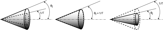
Figure 1.— Different type of relativistic outflows. From left to right: A wide jet, where $\theta_{j}>1/\Gamma$; a sideways-expanding jet, where $\theta_{j}\approx 1/\Gamma$, and a narrow jet, where $\theta_{j}<1/\Gamma$. Since $\theta_{j}$ is unknown, for the wide jet case we will treat the outflow as spherical and refer to isotropic quantities. For the narrow jet we will assume a particular value for $\theta_{j}$ and we will discuss how the results depend on the choice of $\theta_{j}$. (Figure from Barniol Duran et al. 2013).

2.1. The outflow geometry

The geometry of the emitting region is an additional important factor that controls the conditions there. The equipartition arguments presented above can be applied to the non-relativistic (Newtonian) case by setting $\Gamma=1$. In the case of a spherical source, $f_{A}=1$ and $f_{V}\approx 1$. For the relativistic case, the outflow could have a wide opening angle, $\theta_{j}$, comparable or larger than $1/\Gamma$. In such a jet the observer sees only a fraction (an angle of $1/\Gamma$) of the entire jet (this was the reason for the choice of the filling factors in the previous section). We consider two possibilities, a “wide” jet, where $\theta_{j}>1/\Gamma$ (GRB jets are believed to satisfy this condition initially) and a “sideways-expanding” jet (as is the case in the late phase of a GRB afterglow), where $\theta_{j}\approx 1/\Gamma$ (see Fig. 1) . For these two types of jets, assuming the jet is uniform, $f_{A}=1$ and $f_{V}=1$. For any general jet geometry or a non-uniform jet, $f_{A}<1$ and/or $f_{V}<1$. It is harder to imagine how a “narrow” jet with $\theta_{j}<1/\Gamma$ forms as the matter will naturally tend to expand all the way to $1/\Gamma$. Still, in the spirit of a general equipartition approach we do not consider how the outflow formed and just examine what are the possible conditions within the emitting region. In the narrow jet case the observer sees the entire jet while the jet’s emission is beamed into a cone wider than the jet (see Fig. 1), thus for a uniform narrow jet $f_{A}=f_{V}=(\theta_{j}\Gamma)^{2}$. These filling factors introduce factors of

$$(\theta_{j}\Gamma)^{-\frac{16}{17}}\ \ \ \ \ {\rm and}\ \ \ \ \ (\theta_{j}\Gamma)^{-\frac{6}{17}},$$ (8)

in $R_{eq}$ and $E_{eq}$, see eqs. (5) and (7).

It is important to note that the wide and sideways-expanding jets yield exactly the same results since $f_{A}$ and $f_{V}$ are identical. However, for a wide jet, the true number of particles and energy are larger than those calculated above by a factor of $4\Gamma^{2}(1-\cos\theta_{j})$. Clearly, without additional information we cannot determine $\theta_{j}$, therefore, we treat the outflow as spherical and calculate the isotropic equivalent quantities as $N_{e,iso}=4\Gamma^{2}N_{e}$ and $E_{iso}=4\Gamma^{2}E$. Similarly, for the Newtonian spherical case, the total number of emitting particles and the total minimal energy are a factor of 4 larger than obtained in the previous subsection (using $\Gamma=1$), since $N_{e}$ and $E$ in the previous section are obtained for a region with opening angle $\sim 1/\Gamma$.

3. Application to the radio emission of Sw 1644+57

We apply now the formalism derived in Paper I and briefly explained in the previous section to the radio data of Sw 1644+57 (Z11, B12, Z13). This potential tidal disruption event took place at $z=0.354$ for which $d_{L}=5.7\times 10^{27}$ cm (Levan et al. 2011). We focus here on the radio emission that followed the initial soft $\gamma$-rays/hard X-ray emission. The radio data seems to be well described by synchrotron emission with a low energy steep power-law spectrum that requires self-absorbed emission (Z11), and a high energy power-law spectrum for which an index of $p\approx 2.5$ can be derived (B12, Z13). We analyze the radio data of this event in the context of a Newtonian spherical source and also of the three relativistic jet types considered above: wide (isotropic), sideways-expanding and narrow. We also separately consider the effect of including the protons’ energy. We will show that including the protons’ energy has a small effect on the physical parameters of the system and only increases the total minimal energy. Consequently we will initially ignore this term for simplicity and will present its effect only towards the end of this section.

For each observed time, $t$, when there is an available spectrum, we can determine $\nu_{a}$, $\nu_{m}$ and $F_{p}$ (see figs. 2 in B12 and Z13). B12 and Z13 do not find a cooling frequency in their data, and infer it to be much larger than $\nu_{m}$, which makes the simplification of ignoring the electron cooling valid. For Sw 1644+57, the values of $\nu_{a}$ and $\nu_{m}$ (and hence $\eta$) have been obtained by the snap-shot synchrotron broad-band spectrum fitting done by B12 and Z13 (see their tables 2). We will denote this case as $\eta=\eta_{obs}$ to emphasize that we are using the observations of $\nu_{a}$ and $\nu_{m}$ to determine $\eta$. Using the equipartition arguments, we obtain the physical parameters of Sw 1644+57 at each observed time in all the scenarios considered above (see Fig. 2). We calculate the parameters of the outflow as the observed time increases from 5 to 582 days (the time span of the observations in B12 and Z13).

If we assume that the radiating particles are the external medium particles that have been swept-up by the relativistic outflow, and if we assume that all electrons are radiating (one can envision a scenario in which only a fraction of them are emitting), then we can determine the number density of the external medium, $n_{ext}$. The number density of radiating particles in the outflow (in the lab frame), $n_{e}=N_{e}/V$, is related to $n_{ext}$ by $n_{e}=4\Gamma^{2}n_{ext}$ (Blandford & McKee 1976), which yields $n_{ext}=N_{e}/(4f_{V}\pi R^{3}/\Gamma^{2})$. We also notice that for the wide jet case, where we calculate isotropic quantities, $n_{ext}$ is the same as in the sideways-expanding case, since $n_{e}$ remains the same in both cases.

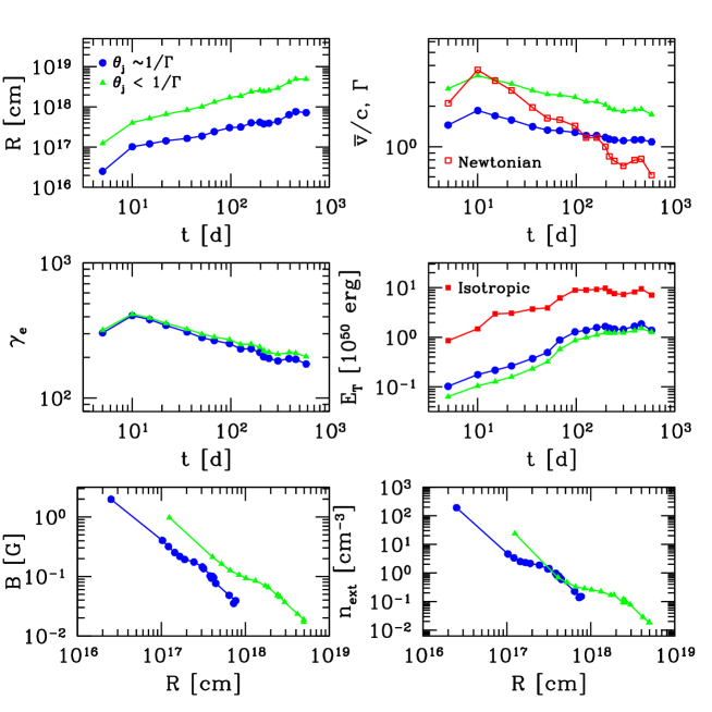
Figure 2.— Physical parameters of Sw 1644+57, assuming equipartition (minimal total energy) and ignoring the protons’ energy, in the following cases: a Newtonian source (red unfilled squares), a relativistic wide jet (red squares, isotropic quantities), a sideways-expanding jet ($\theta_{j}\sim 1/\Gamma$, blue circles) and a narrow jet ($\theta_{j}<1/\Gamma$, using $\theta_{j}=0.1$, green triangles). All quantities have been calculated using the snap-shot synchrotron broad-band spectrum fitting of B12 and Z13, that allows the determination of $\nu_{a}$ and hence of $\eta$, which we call the $\eta=\eta_{obs}$ case. The magnetic field ($B$) corresponds to the co-moving quantity. The velocity in the non-relativistic case ($\bar{v}/c$) is the velocity in units of the speed of light, whereas in the relativistic cases we show the LF of the source ($\Gamma$). No solution is found in the Newtonian spherical outflow case as the obtained velocity exceeds the speed of light (we only show the inferred velocity for this case in the upper right panel). The parameters of the wide jet and the sideways-expanding jet are identical, except for $E_{T}$, for which we show the isotropic quantity. Notice that in all cases $E_{T}$ increases with time by a factor of $\sim 10-20$. The density profiles for both the sideways-expanding and narrow jets exhibit a flattening, but their normalizations are different (right bottom panel).

The results of the equipartition calculation are presented in Fig. 2. We find no consistent Newtonian spherical equipartition solution. The derived radii imply an expansion velocity larger than the speed of light (see Fig. 2). Therefore, we consider only the relativistic scenarios. The relativistic sideways-expanding jet yields $\Gamma\sim 2$, and it decreases with time. The mildly relativistic nature of this jet implies that the ejecta opening angle is large, $\theta_{j}\sim 1$, and the outflow is almost spherical. We also consider a wide jet. We show in Fig. 2 the isotropic total energy in the wide jet case, which is the only different quantity (thus the only one we plot for this case) between the sideways-expanding jet and the wide jet, as explained above. Note that in the wide jet case the isotropic equivalent energy is comparable to the true energy, since $\theta_{j}\lower 2.0pt\hbox{$\,\buildrel\scriptstyle>\over{\scriptstyle\sim}\,$}1$. To account for the possibility of a narrow jet, we consider a relativistic jet with $\theta_{j}=0.1$ (as in B12). We find $\Gamma\sim 3$, and it decreases with time. The radius in this case is larger than the sideways-expanding jet emission radius by about an order of magnitude since $R\sim\theta_{j}^{-16/17}\Gamma^{-6/17}$, see eq. (8), which leads to a larger $\Gamma$ and to a significantly lower magnetic field and external density compared with the sideways-expanding jet case. We will discuss the effect of varying $\theta_{j}$ in Section 3.1.

B12 find $\eta\sim 5$ and $\eta\sim 20$ at 5 and 10 days, respectively. It then monotonically decreases to $\eta\sim 1$ during the time span of the observations. The sudden increase in $\eta$ by a factor of $\sim 4$ between 5 and 10 days (due to a sudden drop in $\nu_{a}$) produces a discontinuity in all the trends we observe in the physical parameters in Fig. 2 during this time span. We find that this is a general feature of all jet types and it is seen in all physical parameters. In particular, between 5 and 10 days we observe a slight increase in LF. This increase in LF is troublesome for a standard afterglow interpretation of the radio data. This sudden increase in $\eta$ between 5 and 10 d stresses the sensitivity of the results on the interpretation of the observations; we will discuss this more in Section 3.3. Keeping this in mind, in the following, we focus on the behavior for $t\lower 2.0pt\hbox{$\,\buildrel\scriptstyle>\over{\scriptstyle\sim}\,$}10$ days.

The overall trends for $10$ d $\lower 2.0pt\hbox{$\,\buildrel\scriptstyle<\over{\scriptstyle\sim}\,$}t\lower 2.0pt\hbox{$\,\buildrel\scriptstyle<\over{\scriptstyle\sim}\,$}200$ d can be explained as follows. B12 find $\nu_{m}\propto t^{-0.9}$, $\nu_{a}\propto t^{-0.2}$, which yields $\eta\propto t^{-0.7}$; they also find that the flux is roughly constant. We find that $\Gamma$ is slightly larger but not much larger than unity. Using the approximate behavior seen for $\Gamma$, $\Gamma\sim t^{-0.2}$ (for the sideways-expanding jet), we use (5) to obtain $R\sim t^{0.3}$, and with it, we find $\gamma_{e}\sim t^{-0.2}$, $B\sim R^{-1.2}$ and $n_{e}\sim R^{-1.1}$, which are the approximate trends seen in Fig. 2. A similar analysis can be done for the narrow jet. Interestingly, for both jets, the sideways-expanding (or wide) and narrow one, the density profile shows a flattening. This flattening can be explained by the fact that the radius varies slowly with time due to the decrease of $\eta$, since $R\propto\eta^{\frac{35}{51}}$, see eq. (5).

For all the scenarios presented above: Wide, sideways-expanding and narrow relativistic jets, the minimal total energy increases almost linearly with time by a factor of $\sim 10-20$ for the first $\sim 200$ days. After $\sim 200$ days, the total minimal energy displays a plateau.

3.1. Different opening angles

The narrow jet results presented above depend on the choice of the opening angle $\theta_{j}$. The results for different values of $\theta_{j}$ can be scaled for this value. The radius is $R\propto\theta_{j}^{-16/17}\Gamma^{-6/17}$, and the total minimum energy is $E\propto\theta_{j}^{-6/17}\Gamma^{-32/17}$, see eq. (8). A different choice of $\theta_{j}$ will lead to a different value of $\Gamma$, since $R\sim t\Gamma^{2}$ for $\Gamma\gg 1$, see eq. (6). With this, we find $E\sim\theta_{j}^{2/5}\sim\Gamma^{-1}$ and $R\propto\theta_{j}^{-4/5}$. These allow us to determine how the radius, LF, and total energy would vary if we choose a different $\theta_{j}$. A smaller $\theta_{j}$ would increase $R$, but it would decrease $E$ and increase $\Gamma$; however, the dependence of $E$ and $\Gamma$ on $\theta_{j}$ is not very strong. Overall varying $\theta_{j}$ has the effect of shifting the curves in Fig. 2, but their shapes are preserved.

3.2. The protons’ energy

If protons are present in the outflow, then their contribution to the total energetics should be taken into account. Fig. 3 depicts, for the narrow jet case, the effect of having hot protons with ten times more energy than the electrons, that is $\bar{\epsilon_{e}}=0.1$ ($\xi=11$). In this case the radius estimate increases only by a factor of $\sim 1.2$ and the total minimal energy increases by a factor of $\sim 4-5$. All other parameters in Fig. 2 are only shifted by a factor of $\lower 2.0pt\hbox{$\,\buildrel\scriptstyle<\over{\scriptstyle\sim}\,$}3$, but their behavior with time (or radius) is unchanged. This is because of the very weak dependence of radius on $\bar{\epsilon_{e}}$.

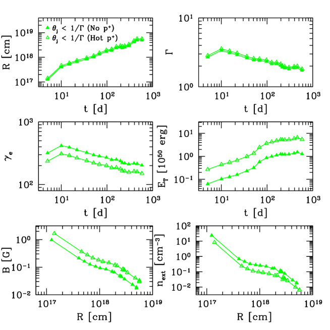
Figure 3.— A comparison of the solution with (unfilled triangles) and without (filled triangles) inclusion of the protons’ energy for the narrow jet case (with $\theta_{j}=0.1$). The inclusion of the protons’ energy increases the total minimal energy by a factor of $\sim 5$; the rest of the parameters are shifted by only a factor of $\lower 2.0pt\hbox{$\,\buildrel\scriptstyle<\over{\scriptstyle\sim}\,$}3$. Similar results can be found for the case of a sideways-expanding (or wide) jet.

3.3. The case of $\eta=1$

To emphasize the importance of detailed radio observations that determine the details of the spectrum, we consider the case when $\nu_{a}$ cannot be determined and set $\eta=1$, that is, we assume that $\nu_{a}\approx\nu_{p}$ as done in Z11. This is clearly an approximation that is useful when there is not enough data to constrain the value of $\nu_{a}$. The results for this case can be found in Fig. 4.

Since $R\propto\eta^{\frac{35}{51}}$, see eq. (5), assuming $\eta=1$ results in slightly lower initial values of $R$ compared with the $\eta=\eta_{obs}$ case. Consequently, the LF is also lower (which allows for a Newtonian solution, although with very high velocities), and both the magnetic field and the external density inferred are larger. Also, since $\eta_{obs}$ decreases to unity over time, it can be seen that the $\eta=\eta_{obs}$ solution relaxes to the $\eta=1$ solution over time (see Figs. 2 and 4); this explains why $R$ varies more slowly with time in the $\eta=\eta_{obs}$ case compared with the $\eta=1$ case.

The main differences between the $\eta=1$ and the $\eta=\eta_{obs}$ solutions are the following. 1. The first allows for a Newtonian solution, although with a high velocity, whereas the second does not. 2. The first shows a density profile with $\propto R^{-2}$, whereas the second shows a weaker decrease with radius and exhibits a plateau. 3. The first shows an almost constant LF with time, whereas the second results in a LF that decreases with time. On the other hand, the main similarity between these two cases is that both show an increase in the total minimal energy over time and that the energy reaches a plateau. Using the values of $\nu_{a}$ in the analysis should provide a better estimate of the physical parameters of Sw 1644+57, therefore, we focus the rest of the analysis on the $\eta=\eta_{obs}$ case (otherwise noted).

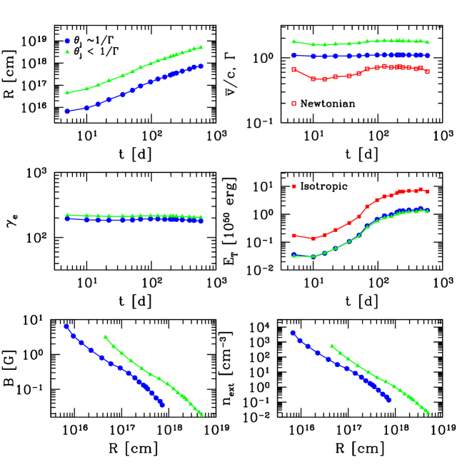
Figure 4.— Physical parameters of Sw 1644+57, assuming equipartition and ignoring the protons’ energy (same symbols as in Fig. 2), using the observed peak flux and peak energy of the spectra in B12 and Z13 and assuming $\nu_{a}\approx\nu_{p}$, that is, $\eta=1$. The resulting LF in the sideways-expanding case is close to unity, therefore, the physical parameters of the Newtonian case are very similar to this case (for this reason, we chose to only show the Newtonian velocity) and the Newtonian total minimal energy is also similar to the isotropic (wide jet) case. Notice that in all cases the total energy increases with time by a factor of $\sim 30$. Here, the density profile is $\propto R^{-2}$, whereas the $\eta=\eta_{obs}$ case shows a weaker decrease with radius and exhibits a plateau.

4. Alternatives to the energy increase

In all cases discussed so far, the puzzling increase of energy over time, which is incompatible with the X-ray emission, is a clear robust characteristic of the equipartition solution. It arises in all solutions, and seems unavoidable. We turn now to explore alternatives to this feature.

4.1. The outflow geometry

One way to avoid the increase in energy is to allow the geometry to vary with time, so as to counteract the energy increase. The main idea is to let $f_{A}$ and/or $f_{V}$ vary so that the energy in eq. (7) remains constant. In the relativistic case, an observer can only see a region within $\sim 1/\Gamma$ from the line of sight, therefore, any change in the observed area should occur within this region, otherwise it would not be detected.

There are numerous ways to vary the geometry. Here, we consider two as a demonstration of the behavior of the system. We can fix $f_{A}$ and let $f_{V}$ vary with time. This can happen if the width of the ejecta varies with time while we keep $\theta_{j}$ constant. Alternatively we can let both $f_{A}$ and $f_{V}$ vary with time, as will be the case if the outflow expands sideways by varying $\theta_{j}$ in the narrow jet case. In the following we explore how $f_{V}$ or $\theta_{j}$ should vary in these two cases in order to keep the total energy constant.

The radius depends extremely weakly on $f_{V}$. Varying $f_{V}$ leaves, effectively, the radius unchanged (see eq. (5)), and consequently also leaves $\Gamma$ unchanged. The minimal total energy, eq. (7), depends on $f_{V}$ as $E\propto f_{V}^{6/17}$. This means that in order that the total energy will not increase by the factor of $\sim 20$ we found in the previous section, $f_{V}$ needs to decrease by the very extreme factor of $\sim 5000$ during the time span of the observations.

The radius in the narrow jet case behaves like $R\propto\theta_{j}^{-16/17}\Gamma^{-6/17}$, see (8). Therefore, a variation of $\theta_{j}$ with time will lead to a large departure from the results obtained when $\theta_{j}$ was kept fixed. The total minimal energy is $E\propto\theta_{j}^{-6/17}\Gamma^{-32/17}$, see eq. (8). As we vary $\theta_{j}$ the radius changes and so will $\Gamma$, see eq. (6), and, as obtained before, $E\sim\theta_{j}^{2/5}\sim\Gamma^{-1}$. Therefore, to avoid the observed increase in total energy by a factor of $\sim 20$, $\theta_{j}$ has to decrease by $\sim 2000$ and $\Gamma$ has to increase by a factor of 20. Clearly this scenario is unreasonable. There is no physical reason why $\theta_{j}$ should decrease by such a large factor. Additionally, the increase in $\Gamma$ is strange, as we expect the outflow to decelerate rather than to accelerate at these late stages of its evolution.

4.2. Beyond equipartition

The total energy increases in all the equipartition scenarios presented above. This is an inevitable result if we assume equipartition. We turn now to consider a scenario in which we force the total energy to be a constant and calculate the physical parameters of the system for this to occur. We will again ignore the protons’ energy, since it only changes the parameters by a small factor as explained earlier.

We use eq. (4) together with eq. (6) to solve for $R$ and $\Gamma$ that keep the total energy constant. We then calculate $\gamma_{e}$, $N_{e}$ and $B$, and determine the microphysical parameters $\epsilon_{e}=E_{e}/E$ and $\epsilon_{B}=E_{B}/E$ as a function of time ($\epsilon_{e}$ is the fraction of the total energy that goes into electrons, whereas $\bar{\epsilon_{e}}$ instead is the fraction of the protons’ energy that goes into electrons).

The total energy should be larger than the minimal total energy obtained in Fig. 2. The minimal $E$ increases until $\sim 2\times 10^{50}$ erg, therefore, we choose this value as the fixed energy. This means that towards the end of the observations we will reach roughly an equipartition solution, whereas earlier on there will be a significant departure from equipartition.

There are two solutions for each one of the scenarios considered: sideways-expanding and narrow jet (as mentioned before, the wide jet case yields same results as the sideways-expanding one). The first solution is a “Poynting flux dominated” solution, in which initially $\epsilon_{B}\sim 1$ and $\epsilon_{e}\ll 1$, namely most of the energy is carried by the magnetic field at the onset of the observations. Eventually, $\epsilon_{e}$ ($\epsilon_{B}$) increases (decreases) with time (see Fig. 5). The second solution is a “baryonic” solution, $\epsilon_{e}\sim 1$ and $\epsilon_{B}\ll 1$ at the beginning and then $\epsilon_{B}$ ($\epsilon_{e}$) increases (decreases) with time (see Fig. 6).

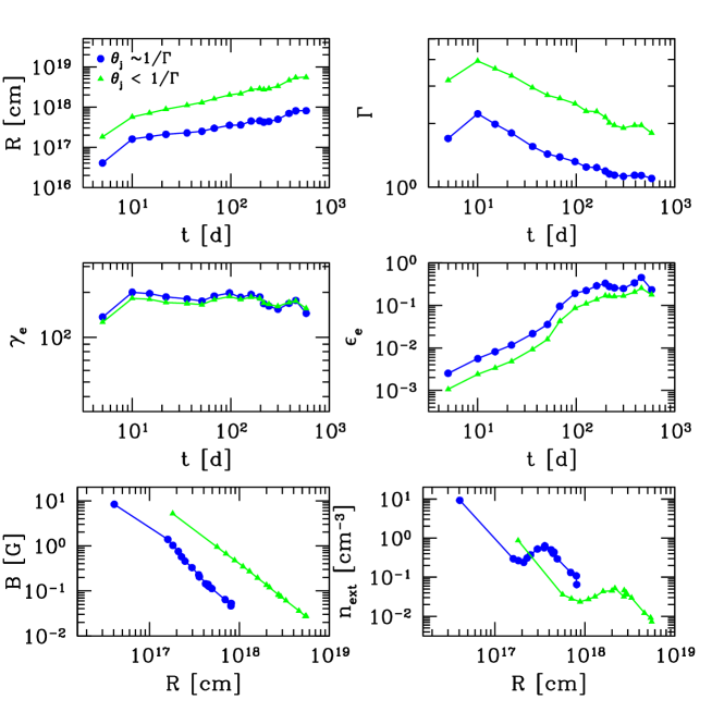
Figure 5.— Physical parameters of Sw 1644+57 for a sideways-expanding jet (solid circles) and for a narrow jet with $\theta_{j}=0.1$ (solid triangles) for a fixed total energy at $E=2\times 10^{50}$ erg (and ignoring the protons energy). All symbols and labels are the same as in Fig. 2. In these cases, initially $\epsilon_{B}\sim 1$ and it slowly decreases with time (not shown) as $\epsilon_{e}$ increases with time as in the right middle panel (see text). Notice that the density profile exhibits a “bump” in both relativistic cases (right bottom panel).

The total energy was fixed to a value that is larger than the equipartition total minimal energy. If the solution is of the magnetically dominated kind, that is, most of the energy is in the magnetic field at the beginning of the observations, then the initial radius needs to be larger, but only slightly larger, than $R_{eq}$ (see Fig. 5). This is because $E_{B}\propto R^{11}$. For this reason, $\epsilon_{e}$ will start out very small, and will later increase. A similar situation arises in the baryonic solution. In this case, the radius will be initially slightly smaller than $R_{eq}$, since $E_{e}\propto R^{-6}$. However, the dependence of $E_{B}$ on radius is so much stronger than the one of $E_{e}$, that the initial $\epsilon_{B}$ will be even smaller than the initial value of $\epsilon_{e}$ in the magnetically dominated solution.

The equipartition solutions presented in Fig. 2 showed two features: An increase in $E$ with time and a flattening in the density profile. When fixing the total energy, as done in this subsection, these two particular features translate to: 1. An increase in $\epsilon_{e}$ ($\epsilon_{B}$) and 2. A small “bump” in the external density (magnetic field); see Fig. 5 (6). These “bumps” are small, the external density and magnetic field increase only by a factor of $\lower 2.0pt\hbox{$\,\buildrel\scriptstyle<\over{\scriptstyle\sim}\,$}4$, still they pose a puzzle to some models as it is not clear why such bumps would arise.

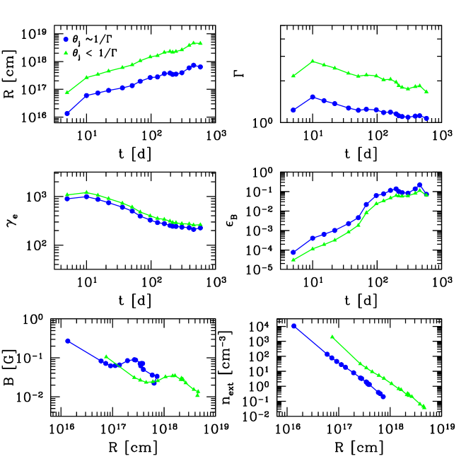
Figure 6.— Physical parameters of Sw 1644+57 for a sideways-expanding jet (solid circles) and for a narrow jet with $\theta_{j}=0.1$ (solid triangles) for a fixed total energy at $E=2\times 10^{50}$ erg (and ignoring the protons energy). All symbols and labels are the same as in Fig. 2. In these cases, initially $\epsilon_{e}\sim 1$ and it slowly decreases with time (not shown) as $\epsilon_{B}$ increases with time as in the right middle panel (see text). Notice that the magnetic field as a function of radius exhibits a “bump” in both relativistic cases (left bottom panel).

Choosing a total energy, $E$, larger than the value used above would affect the results of the sideways-expanding (and wide) jet the following way. In the magnetically dominated (baryonic) solution, both the radius and LF would increase (decrease) as $R\propto E^{1/7}$ and $\Gamma\propto E^{1/14}$ ($R\propto E^{-1/5}$ and $\Gamma\propto E^{-1/10}$), for the highly relativistic case. As done in the previous section, we chose $\theta_{j}=0.1$ to display our results for the case of a narrow jet in Figs. 5 and 6. Choosing a different value of $\theta_{j}$ or a different value of total energy, $E$, would yield $R\propto\theta_{j}^{-5/6}E^{1/12}$ and $\Gamma\propto\theta_{j}^{-5/12}E^{1/24}$ ($R\propto\theta_{j}^{-3/4}E^{-1/8}$ and $\Gamma\propto\theta_{j}^{-3/8}E^{-1/16}$) in the highly relativistic limit for the magnetically dominated (baryonic) case.

The same general conclusions in this subsection apply if we include the effect of the protons’ energy. As noted earlier, the only effect of including the protons energy in the equipartition calculation is to increase the total energy by a constant factor. If we include the protons’ contribution and increase the chosen total energy in Figs. 5 and 6 by this factor, then the parameters in these figures remain unchanged. The precise values of $\epsilon_{B}$ and $\epsilon_{e}$ are modified, but their general trend with time is preserved. In this case, a time-varying $\epsilon_{p}$ is introduced, which is the fraction of the protons energy to the total energy.

5. Discussion

We have applied general equipartition considerations (Paper I) to the radio data of the tidal disruption event candidate, Sw 1644+57, and obtained estimates of the conditions within the emitting region. Before exploring the implications of these finding to different astrophysical scenarios, we remind the reader that the equipartition considerations are based on several key assumptions. In particular, we assume that 1. The jet moves along, or close enough to, the line of sight and 2. The electrons emit only synchrotron radiation and they are slow cooling. The first assumption is reasonable in all models that assume that the jet producing the radio outflow is aligned with the jet producing the X-ray emission and, mainly, in all models in which the radio emission is produced by the same jet that emits the X-rays, otherwise the X-ray energy budget would be too large (see also below). The second assumption is natural in view of simplicity, but see Kumar et al. (2013) for a possible significant deviation from it.

Within the limits of these assumptions, the equipartition arguments yield a robust estimate of the radius of emission, and thus the LF, and of the minimal total energy. The actual total energy could be, of course, much larger if the emission is not maximally efficient. In models with fixed values of $\epsilon_{e}$ and $\epsilon_{B}$ different from the equipartition values of $\epsilon_{e}=0.65$ and $\epsilon_{B}=0.35$, the radius (and LF) are only changed by a small factor and the energy is increased by a constant amount, as explained in Section 2.

The main difference between the LF of the wide (or sideways-expanding ) jet and the narrow jet is the fact that the former shows a lower value of $\Gamma$. For example, at 10 days, $\Gamma\sim 2$ for a wide jet, but $\Gamma\sim 3.5(\theta_{j}/0.1)^{-2/5}$ for a narrow jet with $\theta_{j}\lower 2.0pt\hbox{$\,\buildrel\scriptstyle<\over{\scriptstyle\sim}\,$}0.1$; note that lower values of $\theta_{j}$ yield larger values of $\Gamma$ (see Section 3.1). Thus a narrow jet, being more relativistic, might be consistent with being the same jet that produced the early X-ray emission (MGM12, B12). A wide jet is actually quasi-spherical and mildly relativistic, as suggested by Z11.

5.1. Interpretation of the observed radio data

We stress that the equipartition results depend strongly on the interpretation of the observed radio data and, in particular, on the exact determination of $\nu_{a}$, the self absorption frequency. Different interpretations of the radio data ($\eta=1$ versus $\eta=\eta_{obs}$) yield significantly different physical parameters (see Section 3.3). In particular, an important difference between the $\eta=1$ and $\eta=\eta_{obs}$ cases is that the former shows an approximately constant $\Gamma$ during the time span of the observations, whereas the latter shows a decrease of $\Gamma$ with time. B12 explain the energy increase by invoking a relativistic jet that was launched with a wide range of LFs. $\eta=\eta_{obs}$ is essential for this scenario in which slower material carries more energy which is injected to the shock at a later time after the shock slows down. While these differences stress the importance of detailed observations and careful analysis, they also demonstrate the sensitivity of the results to possible observational errors, or misinterpretation of the data. B12 and Z13 do not provide estimates of the errors in $\nu_{a}$ and $\nu_{m}$ in their spectral fitting. If these errors were to imply $\eta$ values between $1$ and $\eta_{obs}$, we find that there is an ample room for different physical models. Nevertheless we continue the analysis using $\eta=\eta_{obs}$ that seems to employ the best use of the current data.

Within the same context of the interpretation of the data, B12 find a sudden increase in $\eta$ by a factor of $\sim 4$ between 5 and 10 days. This shows up as a discontinuity during this time span in the trends of all physical parameters. This is a general conclusion, which does not depend on the type of jet we consider. In particular, this effect gives rise to a slight increase in LF between 5 and 10 days, which is puzzling for a standard afterglow interpretation. An achromatic break is observed in the radio light curves at $\sim 10$ days (Z11, Wiersema et al. 2012). MGM12 have interpreted this break as the time when the reverse shock has completely crossed the ejecta, which marks the transition between two phases: 1. the phase when the reverse shock is still crossing the ejecta and 2. the phase when the flow settles into the Blandford-McKee self-similar solution. If this interpretation is correct, then there is no reason why the properties of the blast wave (for example, $\epsilon_{B}/\epsilon_{e}$) should be the same in these two phases as considered in our work. It is possible that Rayleigh-Taylor instabilities can mix the ejecta and the shocked medium during the first phase (see, e.g., Levinson 2009, Duffell & MacFadyen 2013), which could in principle vary $\epsilon_{B}/\epsilon_{e}$ for $t<10$ days and cause the slight increase in $\Gamma$ as observed in our results (see, also, Kumar et al. 2013 for a discussion on the observed drop in $\nu_{a}$ between 5 and 10 days). In addition, the achromatic break in the radio light curves is on a similar time scale than that of the energy injection of the jet as seen in the X-rays. This might suggest that both the X-ray and radio components originate from the same jet, since a break in the radio light curve would be coincidental if the X-ray and the radio components originate from different and unrelated outflows (see Discussion in §5.3 and MGM12).

5.2. Comparison with other work

We compare our equipartition calculation for a wide jet with Z11, who considered a wide jet scenario (see Fig. 4) using here $\eta=1$ as they did. The results are consistent within a factor of $\sim 2$ for $t=5-22$ days (see Z11 supplementary Information, table 2). Z11 allow for a proton energy 10 times larger than that in the electrons alone, and so the isotropic energy in Fig. 4 should be multiplied by a factor of $\sim 5$ (see Section 3.2). We also find that $\Gamma$ is close to unity and that it remains constant during this time span. When we continue the calculations to later times we find that additional energy is needed and the overall energy increases by a factor of $\sim 30$ before saturating after about 200 days.

The equipartition results for a narrow jet with $\eta=\eta_{obs}$ and $\theta_{j}=0.1$ (see Fig. 2) should be compared with those presented in B12 (and Z13, see also MGM12). We find that the radius is identical to the one found in fig. 3 in B12; we also obtain a temporal behavior of $R\propto t^{0.6}$ for $t\lower 2.0pt\hbox{$\,\buildrel\scriptstyle>\over{\scriptstyle\sim}\,$}10$ days. In addition, we find $\Gamma\sim 3.5$ and a decrease to $\Gamma\sim 2$ for $t>10$ days. These results approximately agree with B12 ($\Gamma$ would correspond to their value of $\Gamma_{sh}$ in their “afterglow-like” model). We obtain the same density profile as in their fig. 6 (within a factor of $\sim 3$). This density profile, as discussed before, shows a shallower decay compared to the $\eta=1$ case, and it also shows a flattening. We also find an increase in the total energy by a factor of $\sim 20$ as found in B12 and Z13. Z13 find an increase in the total isotropic-equivalent kinetic energy of the jet from $\sim 10^{53}$ erg to $2\times 10^{54}$ erg, which translates to $\sim 5\times 10^{50}$ erg to $\sim 10^{52}$ erg using an opening angle of $\theta_{j}=0.1$ (Z13). The overall behavior is similar and the radius and subsequently $\Gamma$ are comparable. The minimal energy inferred from the equipartition arguments is smaller by a factor of $\sim 50$ compared with the one derived by Z13 (see Fig. 3). Making use of the Z13 values of $\epsilon_{e}=0.1$ and $\epsilon_{B}=0.01$ the total energy would increase by a factor of $\sim 15$ (the protons energy results in a factor of $\sim 10$ and the “non-equipartition” ratio of $\epsilon_{B}/\epsilon_{e}$ results in an additional factor of $\sim 1.5$; see Section 2). Overall, our energy estimate is smaller than the one in Z13 by a factor of $\sim 3$. This comparison with previous radio modeling demonstrates that, indeed, the detailed afterglow-like modeling (MGM12, B12) reduces to the simpler equipartition arguments as long as $\epsilon_{e}\sim\epsilon_{B}$. This is valid, of course as long as the afterglow emission is dominated by just one component: the forward shock in this case (MGM12).

5.3. The X-ray data and the two possible scenarios for the radio data

The total X-ray isotropic equivalent energy of Sw 1644+57 is $E_{x,iso}\approx 3\times 10^{53}$ erg (Bloom et al. 2011, Burrows et al. 2011). Assuming that the energy released in the X-ray band is about one third of the bolometric energy, $\epsilon_{bol}\sim 1/3$ (Bloom et al. 2011), and that the radiation efficiency is $\epsilon_{rad}\sim 0.3$ (although it could be smaller), the total isotropic energy in the jet needed to produce this emission is an order of magnitude larger $E_{j,iso}\approx 3\times 10^{54}(\epsilon_{bol}\epsilon_{rad}/0.1)^{-1}$ erg. The beaming corrected X-ray jet energy is $E_{j}=(E_{j,iso}/2)\max(\theta_{j}^{2},\Gamma_{x}^{-2})$. With $\theta_{j}\sim 1/\Gamma_{x}\sim 0.1$ (Bloom et al. 2011) we find $E_{j}\approx 2\times 10^{52}(\epsilon_{bol}\epsilon_{rad}/0.1)^{-1}(\Gamma_{x}/10)^{-2}$ erg. In the following we compare this energy with the energies involved in the radio emission in the different scenarios.

The radio data of Sw 1644+57 can be explained using two possible scenarios: one involving a narrow jet and the second involving a wide flow. Both scenarios require that the energy of the source increases by a factor of 10-20 from 5 to 200 days, but they differ concerning other aspects of the solution, which we discuss now.

For a narrow jet at 10 days we find a total minimal energy of $E_{r}(10d)\sim 10^{49}(\theta_{j}/0.1)^{2/5}$ erg (see Fig. 2, and Sections 3.1 and 3.2). The energy saturates after $\sim 200$ days at $E_{r}(\lower 2.0pt\hbox{$\,\buildrel\scriptstyle>\over{\scriptstyle\sim}\,$}200d)\sim 2\times 10^{50}$ erg. We find that the ratio of $E_{r}(\lower 2.0pt\hbox{$\,\buildrel\scriptstyle>\over{\scriptstyle\sim}\,$}200d)$ to $E_{j}$ is $E_{r}(\lower 2.0pt\hbox{$\,\buildrel\scriptstyle>\over{\scriptstyle\sim}\,$}200d)/E_{j}\sim 10^{-2}(\theta_{j}/0.1)^{2/5}(\epsilon_{bol}\epsilon_{rad}/0.1)(\Gamma_{x}/10)^{2}$ (this ratio is, of course, even smaller by a factor of 20 for the estimated radio energy at 10 days). This radio energy is only a lower limit on the total energy. Deviations from equipartition, in particular lower values of $\epsilon_{e}$ and $\epsilon_{B}$, result in higher energies and with a significant inefficient radio emission process one can increase the energy so that the radio energy is compatible with the X-ray energy, that is, the same narrow source produces both the X-ray and radio emission, as explained below.

Within the X-ray emitting region $\Gamma$ must be $\geq 1/\theta_{j}$, otherwise the radiation is beamed to a larger angle than $\theta_{j}$ and the energy suppression is not by a factor $\theta_{j}^{2}/2$, which is crucial to reach an overall reasonable energy budget of the X-ray emitting jet. So unless we have an extreme efficiency in the X-ray emission, $E_{j}\approx 2\times 10^{52}(\epsilon_{bol}\epsilon_{rad}/0.1)^{-1}(\Gamma_{x}/10)^{-2}$ erg is a rough estimate of the energy of the fast ($\Gamma\lower 2.0pt\hbox{$\,\buildrel\scriptstyle>\over{\scriptstyle\sim}\,$}10)$ moving material, $E_{fast}\approx E_{j}$. Now, this energy should be comparable to the fast moving material energy that produces the radio at 10 days, $E_{r}(10d)\approx E_{fast}$. As found above, for a narrow jet with $\theta_{j}=0.1$, we have $E_{r}(10d)/E_{j}\sim E_{r}(10d)/E_{fast}\sim 5\times 10^{-4}(\epsilon_{bol}\epsilon_{rad}/0.1)(\Gamma_{x}/10)^{2}$. With deviations from equipartition, $E_{r}(10d)$ would increase by a constant factor (see Section 2). Thus, we find that $\epsilon_{B}\approx 10^{-9}\epsilon_{e}^{-1.5}(\epsilon_{bol}\epsilon_{rad}/0.1)^{2.5}(\Gamma_{x}/10)^{5}$ yields comparable energies in the narrow jet as derived from the early radio data and from X-ray data (however, note the strong dependence on different quantities). Therefore, it is possible that the jet that produced the radio emission and the X-ray emission are one and the same, as required by afterglow-like models (see, MGM12, B12). However, there is an intrinsic problem now. If this is so, then we require now 20 times more energy in slower moving material (to produce the late radio emission) in the model where the energy increase is explained by an outflow with a velocity gradient (B12), $E_{slow}\approx E_{r}(200d)$, and we have a puzzling situation in which, after beaming corrections, the overall energy of the jet is now $E_{slow}\sim 4\times 10^{53}$ erg straining the overall energy budget of the event. Furthermore, this energetic slower moving outflow should not emit any other signal apart from this radio emission. We stress that within this model, comparing $E_{j}$ with $E_{r}(200d)$, the energy of the radio producing matter at $\sim 200$ days is not relevant, since energy was injected by a slow moving material that could not have contributed to the X-ray emission. Unless this paradox is somehow resolved, it seems that this energy injection model is unlikely.

Overall we see that the narrow jet scenario can be based on an “economical” model, which invokes one jet for both the X-ray and radio emission. It requires that the radio emitting regions is very inefficient and strongly out of equipartition as explained above. The increase in the total energy required by the radio data can be explained by energy injected by slower moving material. However, this leads to an intrinsic inconsistency as the energy of the slower moving material, $E_{slow}$, (needed to produce the relatively weak late radio emission) is $\sim 20$ times larger than the energy of the fast moving material, $E_{fast}$, (that produces the strong early X-ray signal). This strains the energy budget of the source and makes this energy injection model questionable. Therefore, it is worthwhile to consider alternative models in which the energy of the magnetic field and/or of the radio emitting electrons increases with time (see Section 4.2) avoiding the need of an extra energy supply to the blast wave.

An additional question that arises in this model is: How can the jet remain narrow and not spread sideways? One may argue that as long as one continues to inject energy over the dynamical time from a very narrow region, then the emission region will appear narrow. However, in this case, when the energy injection stops, then the emission region will start to spread after a dynamical time and we should observe a steepening in the radio light curve. According to the radio modeling, the energy injection seems to stop at $\sim 200$ d; however, the radio light curve does not show any sign of a steepening until the latest observations at $\sim 600$ days (Z13).

In the context of a wide jet, the radio emitting region has a small LF even at early times (see Fig. 2). The inferred opening angle is large ($\theta_{j}\lower 2.0pt\hbox{$\,\buildrel\scriptstyle>\over{\scriptstyle\sim}\,$}1$) and the radio source is quasi-spherical. Clearly, within this context it is meaningless to consider a sideway-expanding jet. Since the outflow is almost spherical, the true energy is close to the isotropic one. We find that the minimal isotropic energy of the radio source is initially $\sim 10^{50}$ erg and it increases by a factor of $\sim 10$ until $\sim 200$ days. Thus, like in the narrow jet case, also here energy has to be added to the radio emitting source during this period. The radio emission is produced by a quasi-spherical and mildly relativistic source, while the X-ray emission is produced by a relativistic and collimated jet as required by the X-ray data (e.g., Bloom et al. 2011). As it is clear from the different geometries required for both emissions, this model requires two independent outflows with the second one (the radio source) not very energetic compared to the X-ray source (provided that the radio emission is not very inefficient).

The overall increase in energy in the wide radio emitting component could be explained, again, by all energy ejected right from the beginning with a velocity gradient. Since here the radio and X-ray sources are different, the inconsistency discussed for the narrow jet does not exist. Alternatively, this wide radio source could be a wind from the super-Eddington accretion disk that exists in the TDE at this stage (e.g., Narayan et al. 2007). One would expect the wind from an accretion disk to be quasi-spherical and at most mildly relativistic. The total energy for the radio source increases almost linearly with time, which would mean that the wind luminosity should be almost constant with time. This is somewhat at odds with the fact that the accretion rate, while remaining super-Eddington, decreases like $t^{-5/3}$ during this period. However, the wind accretion disk properties still remain to be well-understood.

As mentioned before, in both models an energy injection by a factor of $\sim 10-20$ is essential. We can consider, however, time-dependent deviations from equipartition as alternative to the energy increase. In the same context of the two scenarios presented above, instead of invoking a special mechanism to increase the total energy in the radio source, the total energy could have been injected initially primarily in one form (either Poynting flux or baryonic) and later converted from this form to the other (see Section 4.2). This can be viewed as a variation on the scenario in which the excess energy is injected at the beginning but at lower velocities. Therefore, these two options fall into a larger category of energy injection mechanisms, in which the total energy is injected all at once initially, and it is later dissipated by some particular mechanism. Here, the total energy is injected at the beginning, but it is hidden initially in an either predominantly Poynting flux or predominantly baryonic outflow. As above, the “economical” scenario is one in which we have the same narrow jet producing the X-ray and radio emission. The jet, that is launched by a supermassive black hole, is expected to be magnetically dominated. This is also indicated by the lack of SSC emission as noted by Burrows et al. (2011). In their model, the X-rays are produced by the synchrotron process and the lack of a GeV component is a testament of the expected very weak synchrotron-self-Compton component. Therefore, within the context of a total constant energy (and although other scenarios are possible, see Section 4.2), the scenario in which both the X-ray and radio data are produced by the same narrow jet, which is initially Poynting flux dominated and gradually converts its energy to particle energy, seems more natural. Nevertheless, this scenario has also problems. The large energy observed in X-rays requires a large fraction of the total energy in the magnetic jet, which is originally Poynting flux dominated, to be deposited (through magnetic reconnection) in particles. However, the radio data requires a solution where $\epsilon_{e}$ is initially small and the outflow returns to being Poynting flux dominated again, which seems contrived.

The energy increase in the wide jet scenario can also be explained by energy injected initially primarily in one form (either Poynting flux or baryonic) and later converted from this form to the other as explained above. This is an alternate scenario to injecting energy initially with a velocity gradient or an almost constant luminosity from a super-Eddington accretion disk wind. Since in this particular scenario we invoke two different sources (one for the X-ray and one for the radio emission), then this allows for more freedom and avoids the problems discussed in the last paragraph for the narrow jet.

It is interesting to consider, within this time-dependent non-equipartition model, and abandoning the assumption of ignoring the electron cooling, the model suggested by Kumar et al (2013). According to this model, a single narrow jet is responsible for both the X-ray and the radio. All the energy is injected initially, as in the non-equipartition scenario considered above. However, the radio emitting electrons, that arise in the forward shock, do not emit most of their energy via synchrotron. Instead these electrons are cooled by Inverse Compton of the X-ray photons and thus their synchrotron radio flux is strongly suppressed. As the X-ray flux decreases with time, the cooling mechanism weakens. This gives the impression of an apparent energy increase.

Yet another alternative to energy injection could be that the jet was not pointed directly towards us (e.g., Granot et al. 2002), contrary to what was assumed in this work. As the LF decreases and the beaming cone is able to engulf the line of sight, the radio emission might give the impression that energy is increasing. However, a jet that is not pointing towards to us will increase significantly the already strained energy budget required to produce the X-rays. Additionally, we find that $\nu_{m}$ in Sw 1644+57 decreases shallower than expected in the off-axis model (e.g., Margutti et al. 2010). Thus, overall this scenario is quite unlikely.

6. Conclusions

We have applied general relativistic equipartition considerations (Paper I) to the radio data of the tidal disruption event candidate, Sw 1644+57, in the most natural context of standard synchrotron emission. We have shown that this is a powerful tool that reproduces the details of afterglow-like models in a simpler way. It provides a robust estimate of the radius and thus the Lorentz Factor of the radio emitting region, and it gives a minimal total energy required to produce the observed emission. In this context, we have considered a relativistic jet with a wide opening angle as $\theta_{j}>1/\Gamma$ and a narrow one with $\theta_{j}<1/\Gamma$. We considered two possibilities to analyze the synchrotron radio data of Sw 1644+57 depending on the interpretation of the observed spectra. We either take the synchrotron peak frequency to be approximately equal to the self-absorption frequency $\eta=\nu_{p}/\nu_{a}=1$ (Z11) or, alternatively, we take the results of the snap-shot synchrotron broad-band spectrum fitting and determine $\eta_{obs}$ (B12, Z13).

In all cases the minimal total energy of the outflow required to produce the observed radio emission (that is, energy in the magnetic field and radio emitting electrons) increases almost linearly with time for the first $\sim 200$ days, and it reaches a plateau later. The increase in energy is independent of the details of the spectra ($\eta=1$ or $\eta_{obs}$) or of the type of jet considered. This is a robust result that is independent of the analysis and that every model should be able to reproduce. We rule out the possibility that variations in the source geometry are responsible to the apparent increase in energy. The only alternative to this energy increase is if equipartition is not satisfied and all the energy is somehow deployed initially in a form that does not produce synchrotron emission early on.

On the other hand, the details of the variation of the LF with time or the external density profile depend strongly on the interpretation of the radio spectrum. For $\eta=1$, the LF is a constant and the external density profile is $\propto R^{-2}$, whereas for $\eta=\eta_{obs}$ the LF decreases with time and the external density profile is flatter and it displays a plateau (as found by Z11 and B12, respectively). Again, these differences are generic and they are independent of the type of jet (although the normalizations of these different quantities are different). This emphasizes the sensitivity of this analysis to the details of the spectra and stresses the importance of detailed broad-band radio observations.

Two different geometries can explain the radio observations Sw 1644+57: a wide jet and a narrow one. For the first scenario, we find that already at 5 days, when the first radio observation is available, a wide outflow is only mildly relativistic and hence it is quasi-spherical, $\theta_{j}\lower 2.0pt\hbox{$\,\buildrel\scriptstyle>\over{\scriptstyle\sim}\,$}1$. This requires two different sources for the radio and the X-rays producing outflows. Energy considerations suggest that the source of the X-rays is relativistic and collimated (Bloom et al. 2011, Burrows et al. 2011), whereas the radio source is mildly relativistic and quasi-spherical. These differences, and in particular the different geometries, suggest that the X-ray and radio are produced by two different sources. Within the context of an accretion scenario for the TDE, the radio-emitting outflow could arise from mildly relativistic winds emerging from a super-Eddington disk (where the relativistic narrow outflow responsible for the X-ray would arise from a jet that forms in this accretion process).

A second possible scenario involves a narrow jet that is responsible both for the X-ray and later for the radio emission. For a narrow jet, the radio producing outflow is relativistic. This suggests that a common origin for these two sources, which is essential for an afterglow-like model (MGM12, B12), is possible. Note that we have shown here that simple equipartition arguments are strong and replace the need of detailed afterglow-like modeling. The increase in energy in the radio can be explained by energy ejected during the first three days, when most of the X-rays were emitted, but with slower velocities (B12). This flow catches up with the faster (but now decelerating) part of the jet at a later time. This interpretation has problems in its energetics when compared to the energy budget from X-rays. In particular it requires that the energy of the slower moving material, needed to produce the weak late radio emission, is larger by a factor of $\sim 20$ than the energy of the fast moving material that produces the very strong early X-ray emission. The overall (beaming corrected) energy needed is more than $\sim 4\times 10^{53}$ erg and this strongly constraints any TDE model. This motivated us to consider models in which the energy of the magnetic field and/or of the radio emitting electrons increases with time, without having a continuous injection of energy to the blast wave, as considered below.

In the context of the two scenarios presented above, there is an alternative to invoking special mechanisms to increase the total energy in the radio source. It is possible that the total energy required to produce the radio emission is ejected initially predominantly in one form (e.g. Poynting flux) and with time it is converted from this form to the other (e.g baryonic). This is one possibility among many others in which all energy is injected initially and it is accessed at later times. Since the jet that emerges from the massive black hole is expected to be magnetically dominated (e.g., Burrows et al. 2011), a scenario in which the radio data is produced by the same narrow jet that is initially Poynting flux dominated and gradually converts its energy to particle energy is more natural, but also has problems. In addition, the narrowness of the jet at late times poses a challenge to this model and all models that require a narrow outflow. Other scenarios within this alternative are also possible. Within this context, we also mention the recent suggestion by Kumar et al. (2013) that the radio emitting electrons suffer Inverse Compton cooling by the X-ray emission. The increase in the effective $\epsilon_{e}$, as the X-ray flux decreases with time and the cooling mechanism weakens, is responsible for the apparent energy increase in the radio emitting region.

An accurate determination of the angular size of the radio source (or a strong limit) would allow us to discriminate between the two scenarios presented above. This can be done because both models predict different angular sizes (due to their different radii). Moreover, a measurement of proper motion of the radio source would also allow us to discriminate between the two models, since both models predict different LFs. At present, only an upper limit of 0.22 mas on the angular size is available at $\sim 175$ days (B12). This limit is larger than the predicted angular sizes for both wide and narrow jet models at this epoch and it does not provide a meaningful constraint on the opening angle. Future radio observations might be able to provide stronger constraints that could allow us to determine if the jet is narrow or not, and to distinguish between the different physical models.

References

- (1) Barniol Duran R., Nakar E., Piran T., 2013, ApJ, submitted (arXiv:1301.6759) (Paper I)
- (2) Berger E., Zauderer B.A., Pooley G.G., Soderberg A.M., Sari R., Brunthaler A., Bietenholz M.F., 2012, ApJ, 748, 36 (B12)
- (3) Blandford, R.D., McKee C.F., 1976, Phys. Fluids 19, 1130
- (4) Bloom J.S., et al., 2011, Science, 333, 203
- (5) Burrows D.N. et al., 2011, Nature, 476, 421
- (6) Cao D., Wang X.-Y., 2012, ApJ, 761, 111
- (7) Cenko S.B. et al., 2012, ApJ, 753, 77
- (8) Chevalier R.A., 1998, ApJ, 499, 810
- (9) Chevalier R.A., Fransson C., 2006, ApJ, 651, 381
- (10) De Colle F., Guillochon J., Naiman J., Ramirez-Ruiz E., 2012, ApJ, 760, 103
- (11) Duffell P.C., MacFadyen A.I., 2013 (arXiv:1302.7306)
- (12) Granot J., Panaitescu A., Kumar P., Woosley S.E., 2002, ApJ, 570, L61
- (13) Krolik J.H., Piran T., 2011, ApJ, 743, 134
- (14) Kulkarni S.R., et al., 1998, Nature, 395, 663
- (15) Kumar P., Panaitescu A., 2000, ApJ, 541, L51
- (16) Kumar P., Narayan R., 2009, MNRAS, 395, 472
- (17) Kumar P., Barniol Duran R., Bošnjak Ž., Piran T., 2013, MNRAS, submitted
- (18) Levan A.J. et al., 2011, Science, 333, 199
- (19) Levinson A., 2009, ApJ, 705, 213L
- (20) Li Z., Chevalier R.A., 1999, ApJ, 526, 716
- (21) Liu D., Pe’er A., Loeb A, 2012, ApJ, submitted (arXiv:1211.5120)
- (22) Margutti R. et al, 2010, MNRAS, 402, 46
- (23) Metzger B.D., Giannios D., Mimica P., 2012, MNRAS, 420, 3528
- (24) Narayan R., McKinney J.C., Farmer A.J., 2007, MNRAS, 375, 548
- (25) Ouyed R., Staff J.E., Jaikumar P., 2011, ApJ, 743, 116
- (26) Pacholczyk A. G., 1970, Radio Astrophysics (San Francisco: Freeman)
- (27) Piran T., 2004, RvMP, 76, 1143
- (28) Quataert E., Kasen D., 2012, MNRAS, 419, L1
- (29) Sari R., Piran T., Halpern, J.P., 1999, ApJ, 519, L17
- (30) Sari R., Piran T., Narayan R. 1998, ApJ, 497, L17
- (31) Scott M.A., Readhead A.C.S, 1977, MNRAS, 180, 539
- (32) Shklovskii I.S., 1985, Sov. Astron. Lett., 11, 105
- (33) Slysh V.I., 1990, Sov. Astron. Lett., 16, 339
- (34) Soderberg A.M., Brunthaler A., Nakar E., Chevalier R.A., Bietenholz M.F., 2010, ApJ, 725, 922
- (35) Tchekhovskoy A., Metzger B.D., Giannios D., Kelley L.Z., 2013, MNRAS, submitted (arXiv:1301.1982)
- (36) Wiersema K. et al. 2012, MNRAS, 421, 1942
- (37) Zauderer B.A. et al., 2011, Nature 476, 425 (Z11)
- (38) Zauderer B.A., Berger E., Margutti R., Pooley G.G., Sari R., Soderberg A.M., Brunthaler A., Bietenholz M.F., 2013, ApJ, 767, 152 (Z13)