Abstract

We present a new technique for the design of transformation-optics devices based on large-scale optimization to achieve the optimal effective isotropic dielectric materials within prescribed index bounds, which is computationally cheap because transformation optics circumvents the need to solve Maxwell’s equations at each step. We apply this technique to the design of multimode waveguide bends (realized experimentally in a previous paper) and mode squeezers, in which all modes are transported equally without scattering. In addition to the optimization, a key point is the identification of the correct boundary conditions to ensure reflectionless coupling to untransformed regions while allowing maximum flexibility in the optimization. Many previous authors in transformation optics used a certain kind of quasiconformal map which overconstrained the problem by requiring that the entire boundary shape be specified a priori while at the same time underconstraining the problem by employing “slipping” boundary conditions that permit unwanted interface reflections.

OCIS codes: (120.4570) Optical design of instruments; (130.2790) Guided waves; (000.3860) Mathematical methods in physics; (160.3918) Metamaterials.

1 Introduction

In this work, we introduce the technique of transformation inverse design, which combines the elegance of transformation optics [1, 2, 3, 4, 5] (TO) with the power of large-scale optimization (inverse design), enabling automatic discovery of the best possible transformation for given design criteria and material constraints. We illustrate our technique by designing multimode waveguide bends [6, 7, 8, 9, 10, 11, 12, 13, 14, 15, 16, 17, 18] and mode squeezers [19, 17, 18, 20, 21], then measuring their performance with finite element method (FEM) simulations. Most designs in transformation optics use either hand-chosen transformations [3, 13, 14, 22, 23, 24, 25, 26, 27, 28, 29, 11, 19, 12] (which often require nearly unattainable anisotropic materials), or quasiconformal and conformal maps [2, 30, 31, 32, 33, 34, 35, 36, 37, 38, 39, 40, 41, 42, 43, 44, 45, 19, 6, 8, 9, 7, 10, 46, 47, 48] which can automatically generate nearly-isotropic transformations (either by solving partial differential equations or by using grid generation techniques) but still require a priori specification of the entire boundary shape of the transformation. Further, neither technique can directly incorporate refractive-index bounds. On the other hand, most inverse design in photonics involves repeatedly solving computationally expensive Maxwell equations for different designs [49, 50, 51, 52, 53, 54, 55, 56, 57, 58, 59, 60, 61, 62, 63, 64, 65, 66, 67, 68]. Transformation inverse design combines elements of both transformation optics and inverse design while overcoming their limitations. First, the use of optimization allows us to incorporate arbitrary fabrication constraints while at the same time searching the correct space of transformations without unnecessarily underconstraining or overconstraining the problem. Second, instead of solving Maxwell’s equations, we require only simple derivatives to be computed at each optimization step. This is because transformation optics works by using a coordinate transformation $\mathbf{x}^{\prime}(\mathbf{x})$ that warps light in a desired way (e.g. mapping a straight waveguide to a bend, or mapping an object to a point or the ground for cloaking applications [30, 3, 37, 39, 69, 38, 40, 70, 73]) and then employing transformed materials which are given in terms of the Jacobian $\bm{\mathcal{J}}_{ij}=\partial x_{j}^{\prime}/\partial x_{i}$ to mathematically mimic the effect of the coordinate transformation. This transforms all solutions of Maxwell’s equations in the same way (as opposed to non-TO multimode devices which often have limited bandwidth and/or do not preserve relative phase between modes [74, 75, 57, 76, 77, 78, 79, 80, 68, 81, 82]), and is therefore particularly attractive for designing multimode optical devices [83, 84, 85, 31, 17] (such as mode squeezers, expanders, splitters, couplers, and multimode bends) with no intermodal scattering. (Before TO was first used for cloaking, electrostatic cloaking using anisotropic conductivities [72, 71] had been proposed). Examples of such transformations are shown in Fig. 1. For a more comprehensive treatment of the physical and mathematical ideas of transformation media used in this paper, see [73].

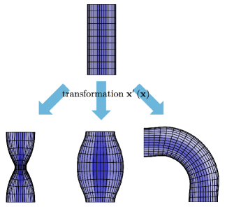
Fig. 1: Three possible applications of transformation optics for multimode waveguides: squeezer, expander, and bend. Dark areas indicate higher refractive index.

One major difficulty with transformation optics is that most functions $\mathbf{x}^{\prime}(\mathbf{x})$ yield highly anisotropic and magnetic materials. In principle, these transformed designs can be fabricated with anisotropic microstructures [86, 87, 88, 26] or naturally birefringent materials [22, 27]. However, in the infrared regime (where metals are lossy) it is far easier to instead fabricate effectively isotropic dielectric materials, provided that the refractive index falls within the given bounds $n_{\mathrm{min}}$ and $n_{\mathrm{max}}$ of the fabrication process (for example, subwavelength nanostructures [39, 38, 69, 40, 33, 86, 89, 90, 91, 44] or waveguides with variable thickness [92, 93, 94, 95, 96, 97]). This requirement means that we would prefer to consider the subset of transformations that can be mapped to approximately isotropic dielectric materials.

The theory of transformation optics with nearly isotropic materials is intimately connected to the subjects of conformal maps (which are isotropic by definition [2, 98, 99]) and quasiconformal maps [which in mathematical analysis are defined as any orientation-preserving transformation with bounded anisotropy (as quantified in Sec. 2.4)]. However, in transformation optics the term “quasiconformal” has become confusingly associated with only a single choice of quasiconformal map suggested by Li and Pendry [30]. In that work, Li and Pendry proposed minimizing a mean anisotropy with “slipping” boundary conditions (defined in Sec. 2.4), which turns out to yield a transformation that is essentially conformal up to a constant stretching (and thus anisotropy) everywhere. This map, which also happens to minimize the peak anisotropy given the slipping boundary conditions [30, 100], is sometimes confusingly called “the quasiconformal map” [6, 34, 36, 38, 40]. However, we point out in Sec. 2.4 that slipping boundary conditions are not the correct choice if one wishes to ensure a reflectionless interface between transformed and untransformed regions. Instead, for interfaces to be reflectionless requires at least continuity of the transformation $\mathbf{x}^{\prime}$ at the interface [101, 102, 103, 85] and, as we show in Sec. 2.3 for the case of isotropic dielectric media, continuity of the Jacobian $\mathcal{J}$ as well. If one fixes the transformation on part or all of the boundary (instead of just the corners) and minimizes the peak anisotropy, the result is called (in analysis) an extremal quasiconformal map [104, 105, 106, 107, 108, 109]. We point out in Sec. 2.2 that this extremal quasiconformal map can never be conformal except in trivial cases. Additionally, previous work in quasiconformal transformation optics underconstrained the space of transformations in one way but overconstrained it in another. Li and Pendry’s method, along with other work on extremal quasiconformal maps in mathematical analysis, assumed that the entire boundary shape of the transformed domain is specified a priori (even if the value of the transformation at the boundary is not specified). In contrast, transformation inverse design allows parts of the boundary shape to be freely chosen by the optimization, only fixing aspects of the boundary that are determined by the underlying problem (e.g. the input/output facets of the boundary in Fig. 1) as explained in Secs. 3.2, allowing a much larger space of transformations to be searched. Also, for such stricter boundary conditions, minimizing the mean anisotropy is not equivalent to minimizing the peak anisotropy [105, 110, 111, 112], and we argue below that the peak anisotropy is a better figure of merit for transformation optics in general.

We solve all of these problems by using large-scale numerical optimization to find the transformation with minimal peak anisotropy that exactly obeys continuity conditions at the boundary with untransformed regions. This allows the input/output interfaces to transition smoothly and continuously into untransformed devices while also satisfying fabrication constraints (e.g. bounds on the attainable refractive indices and bend radiii). A large space of arbitrary smoothly varying transformations (that satisfy the continuity conditions and fabrication constraints) is explored quickly and efficiently by parametrizing in a “spectral” basis [113, 114] of Fourier harmonics and Chebyshev polynomials. The optimized transformation is then scalarized (as in the case of previous work on quasiconformal transformation optics) into an isotropic dielectric material that guides modes with minimal intermodal scattering and loss. In the case of a multimode bend, for which our design was recently fabricated and characterized [115], we achieve intermodal scattering at least an order of magnitude smaller than a conventional non-TO bend.

In Sec. 2.1, we review the equations of transformation optics. In Sec. 2.2, we describe situations where the transformation-designed material can be mapped to isotropic media. In Sec. 2.3, we point out that such isotropic transformations, due to their analyticity, always have undesirable interface discontinuities when coupled into untransformed regions. In Secs. 2.4 and 2.5, we review the techniques of quasiconformal mapping (as used in both the transformation optics and mathematical analysis literature) and scalarization of nearly isotropic transformations. We show that the inherent restrictions of quasiconformal mapping can be circumvented by directly optimizing the map using transformation inverse design. In Secs. 3.1 and 3.2, we design a nearly isotropic transformation for a $90^{\circ}$-bend by perturbing from the highly anisotropic circular bend transformation. In Secs. 3.3 and 3.4, we set up the bend optimization problem and the spectral parameterization. In Sec. 4, we present the optimized structure, which reduces anisotropy by several orders of magnitude compared to the circular TO bend. In Sec. 4.1, we present finite element simulation results comparing our optimized design to the conventional non-TO bend and the circular TO bend. In Secs. 4.2 we show that minimizing the mean anisotropy can lead to pockets of high anisotropy (which in turn leads to greater intermodal scattering) while minimizing the peak does not. In Secs. 4.3, we discuss the tradeoff between the bend radius and the optimized anisotropy. In Sec. 5 we briefly present methods and results for applying transformation inverse design to optimize mode squeezers.

2 Mathematical preliminaries

2.1 Transformation optics

The frequency domain Maxwell equations (fields $\sim e^{-i\omega t}$), without sources or currents, in linear isotropic dielectric media [$\bm{\varepsilon}=\varepsilon(\mathbf{x}),\,\bm{\mu}=\mu_{0}$] are

$$\nabla\times\mathbf{H} =-i\omega\varepsilon(\mathbf{x})\mathbf{E}$$

$$\nabla\times\mathbf{E} =i\omega\mu_{0}\mathbf{H}.$$ (1)

Consider a coordinate transformation $\mathbf{x}^{\prime}\left(\mathbf{x}\right)$ with Jacobian $\mathcal{J}_{ij}=\frac{\partial x_{j}^{\prime}}{\partial x_{i}}$. We define the primed gradient vector as $\nabla^{\prime}\equiv\left(\frac{\partial}{\partial x^{\prime}},\,\frac{\partial}{\partial y^{\prime}},\,\frac{\partial}{\partial z^{\prime}}\right)=\bm{\mathcal{J}}^{-1}\nabla$ and the primed fields as $\mathbf{E}^{\prime}\equiv\bm{\mathcal{J}}^{-1}\mathbf{E}$ and $\mathbf{H}^{\prime}\equiv\bm{\mathcal{J}}^{-1}\mathbf{H}$. One can then rewrite Eq. (1), after some rearrangement [1, 116], as

$$\nabla^{\prime}\times\mathbf{H}^{\prime} =-i\omega\bm{\varepsilon}^{\prime}\mathbf{E}^{\prime}$$

$$\nabla^{\prime}\times\mathbf{E}^{\prime} =i\omega\bm{\mu}^{\prime}\mathbf{H^{\prime}},$$ (2)

where the effects of the coordinate transformation have been mapped to the equivalent tensor materials

$$\bm{\mu}^{\prime}=\mu_{0}\frac{\mathcal{J}^{T}\mathcal{J}}{\det\bm{\mathcal{J}}}\qquad\qquad\bm{\varepsilon}^{\prime}=\varepsilon(\mathbf{x})\frac{\mathcal{J}^{T}\mathcal{J}}{\det\bm{\mathcal{J}}}.$$ (3)

This equivalence has become known as transformation optics (TO). It is actually the specific case of a much more general result from general relativity [118]. For a further discussion of space–time transformations and connections to negative refraction, see [73] and [119].

Most useful applications of TO require that the transformation be coupled to untransformed regions (e.g. the input and output straight waveguides in the case of a bend transformation, or the surrounding air region for the case of a ground-plane cloaking transformation). However, in order for TO to guarantee that the interface between transformed and untransformed regions be reflectionless, the transformation must be equivalent to a continuous transformation of all space that is the identity $\mathbf{x}^{\prime}(\mathbf{x})=\mathbf{x}$ in the “untransformed” regions, as depicted in Fig. 2. More generally, the untransformed regions can be simple rotations or translations, but when examining a particular interface, we can always choose the coordinates to be $\mathbf{x}^{\prime}=\mathbf{x}$ at that interface. It is clear by construction that continuous $\mathbf{x}^{\prime}$ is sufficient for reflectionless interfaces [102, 103, 85], and this is in fact a necessary condition as well [101]. Although a general anisotropic transformation need only have $\mathbf{x}^{\prime}(\mathbf{x})$ continuous at the interface , we show below that an isotropic transformation will also have a continuous $\bm{\mathcal{J}}$ at the interface. These boundary conditions are essential for designing useful transformations without interface reflections.

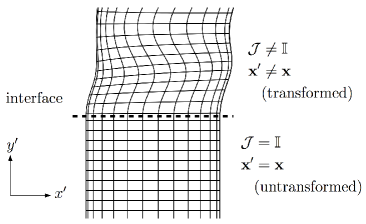
Fig. 2: The interface between the transformed and untransformed region must have $\mathbf{x}^{\prime}$ continuous in order for there not to be any interface reflections.

2.2 Transformations to isotropic dielectric materials

For the vast majority of transformations, the materials in Eq. (3) are anisotropic tensors. However, for certain transformations, the tensors are effectively scalar. Suppose that the transformation $\mathbf{x}^{\prime}(\mathbf{x})$ is 2D ($z^{\prime}=z$ and $\frac{\partial\mathbf{x}^{\prime}}{\partial z}=0$), making $\bm{\mathcal{J}}$ block-diagonal (with the $zz$ element independent of the $xy$ block). Then, the $xy$ block of $\mathcal{J}^{T}\mathcal{J}$ is isotropic if and only if the diagonal elements are equal and the off-diagonal elements vanish:

$$\left|\nabla x^{\prime}\right|^{2}-\left|\nabla y^{\prime}\right|^{2} =0$$

$$\nabla x^{\prime}\cdot\nabla y^{\prime} =0.$$ (4)

In this case, the $\bm{\mathcal{J}}$ part of Eq. (3) becomes

$$\frac{\mathcal{J}^{T}\mathcal{J}}{\det\bm{\mathcal{J}}}=\begin{pmatrix}1\\ &1\\ &&\frac{1}{\det\bm{\mathcal{J}}}\end{pmatrix}.$$ (5)

This isotropy has different implications for transverse-magnetic (TM) polarized modes in 2D (which have $\mathbf{E}=E\hat{z}$ and $\mathbf{H}\cdot\hat{z}=0$) versus transverse-electric (TE) polarized modes (which have $\mathbf{E}\cdot\hat{z}=0$ and $\mathbf{H}=H\hat{z}$). For TM-polarized modes, the fields $\mathbf{E}^{\prime},\,\mathbf{H}^{\prime}$ in the primed coordinate system are also TM-polarized and Eq. (2) becomes

$$\nabla^{\prime}\times\mathbf{H}^{\prime} =-i\omega\frac{\varepsilon(\mathbf{x})}{\det\bm{\mathcal{J}}}\mathbf{E}^{\prime}$$

$$\nabla^{\prime}\times\mathbf{E}^{\prime} =i\omega\mu_{0}\mathbf{H^{\prime}}.$$

Hence, for TM modes, an isotropic transformation can be exactly mapped to an isotropic dielectric material. Similarly, for TE-polarized modes the equivalent material is isotropic and magnetic. However, if $\det\bm{\mathcal{J}}$ varies slowly compared to the wavelengths of the fields, then the transformation can approximately still be mapped to an isotropic dielectric material by making an eikonal approximation (as in [117] Ch. 8.10) and commuting $1/\mu^{\prime}$ with one of the curls in the Maxwell equations. In particular, Eq. (2) can be written:

$$\nabla^{\prime}\times\nabla^{\prime}\times\mathbf{E}^{\prime}=\omega^{2}\varepsilon_{0}\mu_{0}(\det\bm{\mathcal{J}})\mathbf{E}^{\prime}+\mathcal{O}(\nabla\det\bm{\mathcal{J}}),$$

where the last term can be neglected for slowly varying transformations. Because the TM case is conceptually simpler and does not require this extra approximation, we work with it exclusively for the rest of this paper. Also, because the non-trivial aspects of the transformation occur in the $xy$ plane, we hereafter use $\mathcal{J}$ to denote the $xy$ block.

2.3 Conformal maps and uniqueness

If a transformation has an isotropic $\mathcal{J}$, then the transformation preserves angles in the $xy$ plane. Additionally, if $\det\mathcal{J}>0$, then the transformation also preserves handness and orientation. The combination of these two properties is called a conformal map [98], and is the only case where the situation in Sec. 2.2 can be realized. We only consider transformations with $\det\mathcal{J}>0$ in order to restrict ourselves to dielectric materials. Also, a $\det\mathcal{J}>0$ transformation coupled continuously to an untransformed ($\det\mathcal{J}=1$) region would require singularities ($\det\mathcal{J}=0$) at some points. Conformal maps are described by analytic functions, which are of the form $x^{\prime}+iy^{\prime}=w^{\prime}(w)$ (where $w\equiv x+iy$ is the untransformed complex coordinate) and whose real and imaginary parts satisfy the Cauchy–Riemann equations of complex analysis [98, 99].

However, true conformal maps cannot directly be used for transformation optics in typical applications, because of the impossibility of coupling them to untransformed regions with the boundary conditions discussed in Sec. 2.1. In particular, the uniqueness theorem of analytic functions [99, Thm. 10.39] tells us that if $w^{\prime}(w)=w$ in some region, then $w^{\prime}(w)=w$ everywhere (similarly for a simple rotation or translation in some regions).

As a corollary, in the limit where a transformation becomes more and more isotropic in the neighborhood of an interface, it must have a continuous $\mathcal{J}$, not just a continuous $\mathbf{x}^{\prime}(\mathbf{x})$. It is easy to see this explicitly in the example of Fig. 2: continuity of $\mathbf{x}^{\prime}(\mathbf{x})$ at the interface requires that $\frac{\partial\mathbf{x}^{\prime}}{\partial x}=(1,\,0)$ on both sides of the interface, which determines the first row of $\mathcal{J}$. The isotropy of $\mathcal{J}^{T}\mathcal{J}$ then forces $\mathcal{J}=\mathbb{I}$. Therefore, in the sections that follow (where we search for approximately isotropic maps), we will impose the condition of continuous $\mathcal{J}$ as a boundary condition on our transformations. The resulting transformations are nearly isotropic in the interior and exactly isotropic on the interfaces. This condition, discussed at the end of Sec. 2.5, also has the useful consequence of producing a continuous refractive index $n^{\prime}=\sqrt{\varepsilon^{\prime}\mu^{\prime}}$.

2.4 Quasiconformal maps and measures of anisotropy

Because true conformal maps cannot be used, one widely used alternative is to search for a nearly isotropic transformation, which can be approximated by an isotropic material at the cost of some scattering corrections to the exactly transformed modes of the nearly isotropic material. To do this, one must first quantify the measure of anisotropy that is to be minimized. The isotropy condition of Eq. (4) is equivalent to $\lambda_{1}=\lambda_{2}$, where $\lambda_{1}(x,\,y)\geq\lambda_{2}(x,\,y)$ are the two eigenvalues of $\mathcal{J}^{T}\mathcal{J}$. While $\lambda_{1}-\lambda_{2}$ works as a measure of anisotropy, it is convenient for optimization purposes to define differentiable measures that can be expressed directly in terms of the trace and determinant of $\mathcal{J}$, and precisely such quantities have been developed in the literature on quasiconformal maps [109, 120, 105, 121, 104].

A general transformation is an arbitrary function of $x$ and $y$ or, equivalently, an arbitrary function $w^{\prime}(w,\,\bar{w})$, of $w$ and $\bar{w}=x-iy$, which may not be analytic in $w$. The anisotropy can be related to the Beltrami coefficient [109, 105]

$$\mu_{\mathrm{B}}\left(w,\,\bar{w}\right)\equiv\left(\frac{\partial w^{\prime}}{\partial\bar{w}}\right)\left(\frac{\partial w^{\prime}}{\partial w}\right)^{-1}.$$

The term quasiconformal map refers to any map that has bounded $\left|\mu_{\mathrm{B}}\right|<1$, which includes all non-singular sense preserving ($\det\mathcal{J}>0$) transformations. It can be shown that the linear distortion $K$ [104, 105] satisfies

$$K\equiv\frac{1+\left|\mu_{\mathrm{B}}\right|^{2}}{1-\left|\mu_{\mathrm{B}}\right|^{2}}=\sqrt{\frac{\lambda_{1}}{\lambda_{2}}}\geq 1.$$

Various other measures of anisotropy have been defined in the grid generation literature [122, 123], including the Winslow and Modified Liao functionals, which are given by $\Phi\equiv\int\mathrm{d}^{2}x\,(K+\frac{1}{K})$ and $\Phi\equiv\int\mathrm{d}^{2}x\,(K^{2}+\frac{1}{K^{2}})$, respectively. However, for the rest of this work we refer to the quantity $\mathbb{K}-1\geq 0$ as the “anisotropy”, where $\mathbb{K}$ is the distortion function [104, 105], defined as

$$\mathbb{K}\left(x,\,y\right)\equiv\frac{1}{2}\left(K+\frac{1}{K}\right)=\frac{\mathrm{tr}\mathcal{J}^{T}\mathcal{J}}{2\det\mathcal{J}}\geq 1.$$ (6)

The tensor $\frac{\mathcal{J}^{T}\mathcal{J}}{\det\mathcal{J}}$ is known as the distortion tensor [105].

As mentioned in the introduction, an extremal quasiconformal map is one that minimizes the peak anisotropy, given the shape of the transformed region and the values of the transformation on some or all of the boundary [104, 120, 109, 105]. Because $\mathbb{K}$, $\mathbb{K}-1$, $K$, and $\left|\mu_{\mathrm{B}}\right|$ are all monotonic functions of one another, they are equivalent for the purpose of finding an extremal quasiconformal map. However, $\mathbb{K}$ is numerically convenient because it is a differentiable function of the entries of $\mathcal{J}$. These quantities are not generally equivalent for minimizing the mean anisotropy [105, 110, 111, 112], and we argue in Sec. 4.2 that the peak anisotropy is a better figure of merit. However, in the special case where the value of the transformation is only fixed at the corners of the domain and is allowed to vary freely in between (a “slipping”’ boundary condition), Li and Pendry showed that it is equivalent to minimize the mean (either Winslow or modified-Liao) or the peak anisotropy, and that these yield a constant-anisotropy map (a uniform scaling of a conformal map) [100] that they and other authors have used for transformation optics [31, 32, 33, 34, 35, 36, 37, 38, 39, 40, 41, 42, 43, 44, 45, 19, 6]. However, the slipping boundary will generally lead to reflections at the interface between the transformed and untransformed regions because of the resulting discontinuity in the transformation, which can only be reduced by making the transformation domain very large in cases (e.g. cloaking) with localized deformations. In order to design compact transformation-optics devices, especially for applications such as bends where the deformation is nonlocalized, we will instead impose continuity of the transformation and/or its Jacobian on the input/output facets of the domain, while at the same time allowing the shape of some or all of the boundary to vary (unlike all previous work on quasiconformal maps, to our knowledge).

2.5 Scalarization errors for nearly isotropic materials

The minimum-anisotropy quasiconformal map is then scalarized (as in [30]) by approximating it with an isotropic dielectric material. As shown in Sec. 2.2, a perfectly isotropic 2D transformation of a geometry with an isotropic dielectric material that guides TM modes $\mathbf{E}_{0},\,\mathbf{H}_{0}$ can be mapped to a transformed material and geometry that is also isotropic dielectric and guides TM modes $\mathbf{E}_{0}^{\prime},\,\mathbf{H}_{0}^{\prime}$. This is exact for $\mathbb{K}=1$, but for a nearly isotropic transformation with $\mathbb{K}>1$, the equivalent permeability is $\bm{\mu}^{\prime}=\mathbb{I}+\Delta\bm{\mu}$, where the anisotropic part $\Delta\bm{\mu}$ is proportional to $\mathbb{K}-1$ to lowest order. While $\Delta\bm{\mu}^{\prime}\neq 0$ cannot be fabricated using dielectric gradient index processes, one can neglect this small correction so that the actual fabricated material has permeability $\bm{\mu}_{\mathrm{approx}}^{\prime}=\mathbb{I}$. In practice, we absorb any $\Delta\bm{\mu}^{\prime}$ into $\varepsilon^{\prime}$ by multiplying $\varepsilon^{\prime}$ by the average eigenvalue of $\bm{\mu}^{\prime}$

$$\left\langle\bm{\mu}^{\prime}\right\rangle=\frac{\lambda_{1}+\lambda_{2}}{2\sqrt{\lambda_{1}\lambda_{2}}}=\frac{\mathrm{tr}\mathcal{J}^{T}\mathcal{J}}{2\det\mathcal{J}}$$ (7)

but this does not change the $\mathcal{O}\left(\mathbb{K}-1\right)$ error.

A Born approximation [124, 125, 126] tells us that, given an exact transformation with no scattering, any small error of $\Delta\bm{\varepsilon}$ and $\Delta\bm{\mu}$ will generically lead to scattered fields with magnitudes of $\mathcal{O}(\left|\Delta\bm{\varepsilon}\right|+\left|\Delta\bm{\mu}\right|)$ and scattered power of $\mathcal{O}(\left|\Delta\bm{\varepsilon}\right|^{2}+\left|\Delta\bm{\mu}\right|^{2})$. The modes of the approximate scalarized material $\bm{\mu}_{\mathrm{approx}}^{\prime},\,\varepsilon_{\mathrm{approx}}^{\prime}$ are then the exact guided modes plus scattered power corrections of $\mathcal{O}(|\Delta\bm{\mu}|^{2})=\mathcal{O}[(\mathbb{K}-1)^{2}]$.

A similar analysis explains why we must explicitly impose continuity of $\mathcal{J}$ at the input/output facets of the domain. As explained in Sec. 2.3, a purely isotropic transformation in the neighborhood of the interface, along with a continuity of $\mathbf{x}^{\prime}$, would automatically yield continuous $\mathcal{J}$, so one might hope that minimizing anisotropy would suffice to obtain a nearly continuous $\mathcal{J}$. Unfortunately, as we show in the Appendix, the resulting discontinuity in $\det\mathcal{J}$ (and hence the discontinuity in the refractive index) is of order $\mathcal{O}(\sqrt{\mathbb{K}-1})$, which would lead to $\mathcal{O}(\mathbb{K}-1)$ power loss due to reflections, much larger than the $\mathcal{O}[\left(\mathbb{K}-1\right)^{2}]$ power scattering from anisotropy in the interior. This would make it pointless to minimize the anisotropy in the interior, since the boundary reflections would dominate. In fact, our initial implementation of the bend optimization in Sec. 3.4 did not enforce continuity of $\mathcal{J}$, and we obtained a large $2\%$ index discontinuity at the endfacets for $\max_{\mathbf{x}}\mathbb{K}-1\approx 0.0005$. Therefore, in Sec. 3.4 we impose continuity of $\mathcal{J}$ explicitly.

2.6 General optimization of anisotropy

In this paper, we directly minimize $\mathbb{K}$ using large-scale numerical optimization while keeping track of constraints on the transformation $\mathbf{x}^{\prime}$ and its Jacobian $\mathcal{J}$, as well as the engineering fabrication bounds $n_{\mathrm{min}}$ and $n_{\mathrm{max}}$. By using numerical optimization, we can in principle achieve both a lower mean anisotropy and a lower peak anisotropy than by traditional quasiconformal mapping, since the optimization is also free to vary the boundary shape (with at most the input/output interfaces fixed, although in some cases their locations and shapes are allowed to vary as well). The minimization problem can be written, for example, as

$$\min_{\mathbf{x}^{\prime}(\mathbf{x})}\left\|\mathbb{K}(\mathbf{x})\right\|\;\mathrm{subject\,to}\;\begin{cases}\mathbf{x}^{\prime},\,\mathcal{J}\,\mathrm{continuous\,at\,input/output\,interfaces}\\ n_{\mathrm{min}}\leq n^{\prime}(\mathbf{x})\leq n_{\mathrm{max}}\end{cases},$$ (8)

where $\left\|\mathbb{K}(\mathbf{x})\right\|$ is a functional norm taken over the domain of $\mathbf{x}^{\prime}(\mathbf{x})$. We consider two possible norms: the $L_{1}$ norm (the mean $\left\langle\mathbb{K}\right\rangle_{\mathbf{x}}$), and the $L_{\infty}$ norm ($\max_{\mathbf{x}}\mathbb{K}$). We show in Sec. 4.2 that minimizing the mean can lead to pockets of high anisotropy which can cause increased scattering. Directly optimizing the peak anisotropy on the other hand, avoids such pockets while simultaneously keeping the mean nearly as low. The continuity of $\mathbf{x}^{\prime}$ and $\mathcal{J}$ at the input/output interfaces, as well as other constraints on the interface locations, are imposed implicitly by the parametrization of $\mathbf{x}^{\prime}(\mathbf{x})$ (as explained in Sec. 3.4).

3 Multimode Bend design

In this section, we design a bend transformation (depicted in Fig. 3) using general methods to (locally) solve the optimization problem of Eq. (8). In contrast, previous work on TO bend design either utilized materials that were either anisotropic or consisted of multiple stacked isotropic layers [11, 12, 13, 14, 15, 17, 18] or employed slipping boundary conditions [6, 7, 8, 9, 10] (which result in endfacet reflections when coupled to untransformed waveguide).

3.1 Simple circular bends

First, we consider a simple circular bend transformation (which we refer to hereafter as the circular TO bend) that maps a rectangular segment of length $L$ and width unity (in arbitrary distance units to be determined later) into a bend with inner radius $R$ and outer radius $R+1$ (as shown in Fig. 3). For convenience, we choose the untransformed coordinates to be $R\leq x\leq R+1$ and $-\frac{L}{2}\leq y\leq\frac{L}{2}$, with the untransformed segment length $L=\frac{\pi R}{2}$ equal to the inner arclength of the bend. The transformation $\mathbf{x}^{\prime}(\mathbf{x})$ can be written as

$$x^{\prime} =r\,\cos\theta$$

$$y^{\prime} =r\,\sin\theta$$

$$z^{\prime} =z,$$ (9)

where $r=x$ and $\theta=\frac{y}{R}$. While $\mathbf{x}^{\prime}$ is continuous at the input/output interfaces $y=\pm\frac{L}{2}$, one issue is that $\mathcal{J}$ is not continuous there, which can be seen from $\det\mathcal{J}=\frac{x}{R}\neq 1$. Another issue is that $\bm{\mu}^{\prime}\neq\mu_{0}\mathbb{I}$ is highly anisotropic. The anisotropy for this transformation is $\mathcal{\mathbb{K}}(x,\,y)-1=\frac{x}{2R}+\frac{R}{2x}-1$, which has a peak value $\max_{\mathbf{x}}\mathbb{K}-1\approx\frac{1}{2R^{2}}$ for $R\gg 1$ at the outer radius $x=R+1$. Note that one can instead choose $r=\exp(\frac{\pi x}{2L})$, which gives the conformal bend $x^{\prime}+iy^{\prime}=\exp[\frac{\pi}{2L}(x+iy)]$. As explained in Sec. 2.3, this map has zero anisotropy, but neither $\mathbf{x}^{\prime}$ nor $\bm{\mathcal{J}}$ are continuous at the input/output interfaces, leading to large reflections there.

3.2 Generalized bend transformations

In order to address the problems of the circular TO bend, we look for minimum anisotropy and continuous-interface transformations of the form of Eq. (9), where the intermediate polar coordinates are now arbitrary functions $r(x,\,y)$ and $\theta(x,\,y)$. The ratio $L/R$ is now an optimization parameter. The Jacobian then satisfies

$$\mathrm{\mathrm{tr}}\mathcal{J}^{T}\mathcal{J} =\left|\nabla r\right|^{2}+\left|r\nabla\theta\right|^{2}$$

$$\det\mathcal{J} =\left|\nabla r\times r\nabla\theta\right|.$$

We find that the optimization always seems to prefer a symmetric bend (and if the optimum is unique, it must be symmetric), so we impose a mirror symmetry in order to halve our search space:

$$r(x,\,y) =r(x,\,-y)$$

$$\theta(x,\,y) =-\theta(x,\,-y).$$ (10)

We also require interface continuity of $\mathbf{x}^{\prime}$ and $\mathcal{J}$ (as discussed in Sec. 2.3), which give the conditions at $y=\pm\frac{L}{2}$:

$$r =x$$

$$\theta =\pm\frac{\pi}{4}$$

$$\frac{\partial r}{\partial y} =0$$

$$\frac{\partial\theta}{\partial y} =\frac{1}{x}.$$ (11)

3.3 Numerical optimization problem

Besides minimizing the objective function $\mathbb{K}$, the optimization must keep track of several constraints. First, any fabrication method will bound the overall refractive index $n^{\prime}$ to lie between some values $n_{\mathrm{min}}$ and $n_{\mathrm{max}}$. We choose units so that the width of the transformed region is unity ($R\leq x\leq R+1$), and consider transforming a straight waveguide of width $\Delta_{\mathrm{w}}<1$. $\Delta_{\mathrm{w}}$ should be small enough so that the exponential tails of the waveguide modes are negligible outside the transformed region. In the straight waveguide segment to be transformed (as well as the straight waveguides to be coupled into the input and output interfaces of the bend), $n(\mathbf{x})$ is high in the core $\left|x-R-\frac{1}{2}\right|<\frac{\Delta_{\mathrm{w}}}{2}$ and low in the cladding $\left|x-R-\frac{1}{2}\right|>\frac{\Delta_{\mathrm{w}}}{2}$. For convenience, we write this refractive index as a product $n(\mathbf{x})=n_{0}p(x)$ of an overall refractive index $n_{0}$ and a normalized profile $p(x)$ that is unity in the cladding and some value greater than unity in the core (determined by the ratio of the high and low index regions of the straight waveguide). The transformed refractive index is given by

$$n^{\prime}\left(\mathbf{x}\right)=\sqrt{\varepsilon^{\prime}\mu^{\prime}}=n_{0}p\left(x\right)\sqrt{\frac{\mathrm{tr}\mathcal{J}^{T}\mathcal{J}}{2\left(\det\mathcal{J}\right)^{2}}}$$

where the average eigenvalue $\mu^{\prime}$ of the magnetic permeability Eq. (7) has been absorbed into the dielectric index. The overall refractive-index scaling $n_{0}$ is then allowed to freely vary as a parameter in the optimization. Second, like the circular TO bend, the optimum TO bend is expected to have a tradeoff between the bend radius and anisotropy. Because of this expected tradeoff, we can choose to either minimize $R$ while keeping $\mathbb{K}$ fixed, or minimize $\mathbb{K}$ while keeping $R$ fixed. We focus on the latter choice, since the bend radius is the more intuitive target quantity to know beforehand. Also, we find empirically that optimizing $\mathbb{K}$ converges much faster than optimizing $R$ while yielding the same local minima.

With these constraints, there are several ways to set up the optimization problem, depending on which norm we are minimizing. One method is to minimize the peak anisotropy $\max_{\mathbf{x}}\mathbb{K}$ with $\mathbf{x}\in G$ for some grid $G$ of some points to be defined in Sec. 3.4. However, the peak (the $L_{\infty}$ norm) is not a differentiable function of the design parameters, so it should not be directly used as the objective function. Instead, we perform a standard transformation [114]: we introduce a dummy variable $t$ and indirectly minimize the peak $\mathbb{K}$ using a differentiable inequality constraint between $t$ and $\mathbb{K}(\mathbf{x})$ at all $\mathbf{x}\in G$:

$$\min_{r(\mathbf{x}),\,\theta(\mathbf{x}),\,n_{0},\,L,\,t}t\;\mathrm{subject\,to}:\;\begin{cases}\mathrm{continuity\;conditions}\;\,\ref{eq:symmetry},\,\ref{eq:continuity}\\ n_{\mathrm{min}}\leq n_{0}p\left(x\right)\sqrt{\frac{\mathrm{tr}\mathcal{J}^{T}\mathcal{J}}{2\left(\det\mathcal{J}\right)^{2}}}\leq n_{\mathrm{max}}\,\mathrm{for\,}\mathbf{x}\in G\\ R=R_{0}\\ \mathcal{\mathbb{K}}(\mathbf{x})\leq t\,\mathrm{for\,}\mathbf{x}\in G\end{cases}.$$ (12)

For comparison, we explain in Sec. 4.2 why the $L_{\infty}$ norm is better to minimize than the $L_{1}$ norm (the mean anisotropy).

The minimization of the $L_{1}$ norm, $\left\langle\mathbb{K}\right\rangle_{\mathbf{x}}=\int\mathbb{K}\,\mathrm{d}x\,\mathrm{d}y/\mathrm{area}$ [which is differentiable in terms of the parameters $r(\mathbf{x})$, $\theta(\mathbf{x})$, $n_{0}$, and $L$] is implemented as

$$\min_{r(\mathbf{x}),\,\theta(\mathbf{x}),\,n_{0},\,L}\left\langle\mathbb{K}\right\rangle_{\mathbf{x}}\;\mathrm{subject\,to}:\;\begin{cases}\mathrm{continuity\;conditions}\;\,\ref{eq:symmetry},\,\ref{eq:continuity}\\ n_{\mathrm{min}}\leq n_{0}p\left(x\right)\sqrt{\frac{\mathrm{tr}\mathcal{J}^{T}\mathcal{J}}{2\left(\det\mathcal{J}\right)^{2}}}\leq n_{\mathrm{max}}\;\mathrm{for\,}\mathbf{x}\in G\\ R=R_{0}\end{cases}.$$ (13)

We use the circular bend $r=x,\,\theta=\frac{\pi y}{2L}=\frac{y}{R}$ as a starting guess, and search the space of general transformations $r(\mathbf{x}),\,\theta(\mathbf{x})$ by perturbing from this base case. (We only perform local optimization; not global optimization, but comment in Sec. 4.3 on a simple technique to avoid being trapped in poor local minima.) As explained in Sec. 3.4, the perturbations will be parameterized such that the symmetry and continuity constraints are satisfied automatically. Figure 3 shows a schematic of the bend transformation optimization process. First, the straight region is mapped to a circular bend. Then, the intermediate polar coordinates $r$ and $\theta$ for every point $\mathbf{x}$ are perturbed, using an optimization algorithm described at the end of Sec. 3.4, and the desired norm (either $L_{1}$ and $L_{\infty}$) of the anisotropy is computed. This process is repeated at each optimization step until the structure converges to a local minimum in $\left\|\mathcal{\mathbb{K}}\right\|$.

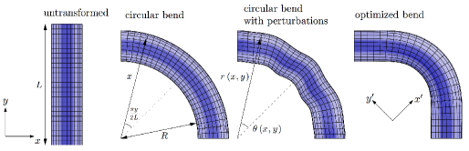
Fig. 3: In the transformation process, the untransformed straight waveguide is bent, perturbed, and optimized. Darker regions indicate higher refractive index

3.4 Spectral parameterization

To faciliate efficient computation of the objective and constraints, the functions $r$ and $\theta$ can be written as the circular bend transformation plus perturbations parametrized in the spectral basis [113, 114]:

$$r\left(x,\,y\right) =x+\sum_{\ell,\,m}^{N_{\ell},\,N_{m}}C_{\ell m}^{r}T_{\ell}(2x-2R-1)\,\cos\frac{2m\pi y}{L}$$

$$\theta\left(x,\,y\right) =\frac{\pi y}{2L}+\frac{1}{x}\sum_{\ell,\,m}^{N_{\ell},\,N_{m}}C_{\ell m}^{\theta}T_{\ell}(2x-2R-1)\,\sin\frac{2m\pi y}{L},$$ (14)

where the coordinate $2x-2R-1$ has been centered appropriately for the domain $\left[-1,\,1\right]$ of degree-$\ell$ Chebyshev polynomials $T_{\ell}$. The sines and cosines have been chosen to satisfy the mirror-symmetry conditions of Eq. (10). The sine series also automatically satisfies the second continuity condition of Eq. (11). In order to satisfy the rest of the conditions, the following constraints are also imposed:

$$\sum_{m}^{N_{m}}C_{\ell m}^{r}\left(-1\right)^{m} =0$$

$$\sum_{m}^{N_{m}}C_{\ell m}^{\theta}\left(-1\right)^{m}m =\begin{cases}\frac{L}{8\pi}-\frac{R}{4}-\frac{1}{8},&\ell=0\\ -\frac{1}{8},&\ell=1\\ 0,&\ell\geq 2\end{cases}.$$ (15)

These equations are solved to simply eliminate the $C_{\ell N_{m}}^{r,\,\theta}$ coefficients before optimization.

This spectral parametrization has several advantages over finite-element discretizations such as the piecewise-linear parameterization of [104]. First, the spectral basis converges exponentially for smooth functions [113]. We found that only a small number ($N_{\ell}\times N_{m}<100$) of spectral coefficients $C^{r,\,\theta}$ are needed to achieve very low-anisotropy ($\mathcal{\mathbb{K}}-1\approx 10^{-4}$) transformations. Second, if the fabrication process favors slowly varying transformations (or if these are needed to make the eikonal approximation for the TE polarization, as in Sec. 2.2), this constraint may be imposed simply by using smaller $N_{\ell}$ and $N_{m}$.

With this spectral parameterization, the formulation of the optimization problem Eq. (12) becomes

$$\min_{\left\{C_{\ell m}^{r,\theta}\right\},\,n_{0},\,L,\,t}t\;\mathrm{subject\,to}:\;\begin{cases}\mathrm{constraint\,\ref{eq:cconstraint}}\\ n_{\mathrm{min}}\leq n_{0}p\left(x\right)\sqrt{\frac{\mathrm{tr}\mathcal{J}^{T}\mathcal{J}}{2\left(\det\mathcal{J}\right)^{2}}}\leq n_{\mathrm{max}}\,\mathrm{for\,}\mathbf{x}\in G\\ R=R_{0}\\ \mathbb{K}(\mathbf{x})\leq t\,\mathrm{for\,}\mathbf{x}\in G\end{cases}.$$ (16)

The local optimization was performed using the derivative-free COBYLA non-linear optimization algorithm [127, 128] in the NLopt package [129]. In principle, we can make the optimization faster by analytically computing the derivatives of the objective and constraints with respect to the design parameters and using a gradient-based optimization algorithm, but that is not necessary because both $\mathrm{tr}\mathcal{J}^{T}\mathcal{J}$ and $\det\mathcal{J}$, which determine all the non-trivial objective and constraint functions in this optimization problem, are so computationally inexpensive to evaluate that the convergence rate is not a practical concern.

4 Optimization results

4.1 Minimal peak anisotropy

A $\min\left\|\mathbb{K}\right\|_{\infty}$ design is shown in Fig. 4, along with the scalarized circular TO bend for comparison. The bend radius was $R=2$ and the number of spectral coefficients was $N_{\ell}=5,\,N_{m}=8$. The objective and constraints were evaluated on a $100\times 140$ grid $G$ in $\mathbf{x}$ (Chebyshev points in the $x$ direction and a uniform grid in the $y$ direction). This design had $\max_{\mathbf{x}}\mathbb{K}-1\approx 5\times 10^{-4}$ and mean $\left\langle\mathbb{K}\right\rangle-1\approx 10^{-4}$. In comparison, the circular TO bend of the same radius has $\max_{\mathbf{x}}\mathcal{\mathbb{K}}-1\approx 0.1$ and $\left\langle\mathbb{K}\right\rangle-1\approx 10^{-2}$.

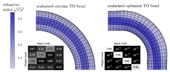
Fig. 4: Optimization decreases anisotropy by a factor of $10^{-4}$, while dramatically improving the scattered-power matrix.

The $R=2$ optimized design structure was compared in finite-element Maxwell simulations (using the FEniCS code [130]), with the conventional non-TO bend [simply bending the waveguide profile around a circular arc with $n^{\prime}(\mathbf{x}^{\prime})=n(\mathbf{x})$] and the scalarized circular TO bend. The four lowest-frequency modes of a multimode straight waveguide were injected at the input interface $y=\frac{L}{2}$, and the scattered-power matrix $T$ was computed using the measured fields at the output interface $y=-\frac{L}{2}$. The scattered-power matrix is defined as

$$T_{ij}=\left|\intop_{R}^{R+1}\mathrm{d}x\,\hat{\theta}\cdot\left(\mathbf{E}_{j}^{0}\times\mathbf{H}_{i}\right)\right|_{y=-\frac{L}{2}}^{2},$$

where $-\hat{\theta}$ is the propagation direction of the guided modes, $\mathbf{E}_{j}^{0}$ is the normalized electric field of the $j$th exactly guided mode of the non-scalarized material $\left(\bm{\mu}^{\prime},\,\varepsilon^{\prime}\right)$, and $\mathbf{H}_{i}$ is the actual magnetic field of the approximate scalarized material at the interface after injecting a normalized mode $\mathbf{E}_{i}^{0}$ at the input interface. This makes $T_{ij}$ equal to the power scattered into the $j$th output mode from the $i$th input mode. For a straight waveguide, which has no intermodal scattering, $T=\mathbb{I}$. Figure 4 shows a dramatically improved $T$ for the scalarized and optimized TO bend compared to the scalarized circular TO bend. [The rows and columns of $T$ for the circular bend add up to less than one because some power has either been scattered out of the waveguide entirely, or some power has been scattered into fifth or higher-order modes. The rows and columns of $T$ for the optimized bend add up to nearly 1, with the small deficiency due to the $\mathcal{O}\left(\mathbb{K}-1\right)$ out-of-bend and higher-order intermodal scattering as well as mesh-descretization error.]

The electric-field profiles for the fundamental mode, displayed in Fig. 5, show a dramatic difference in the performance of the optimized structure versus the other structures. Both the conventional and circular TO bend show heavy intermodal scattering in the bend region, while the optimized transformation displays very little scattering.

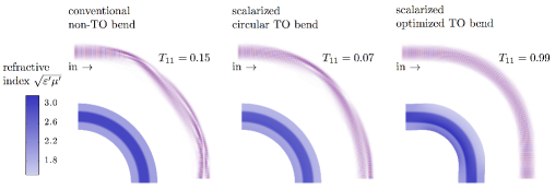
Fig. 5: FEM field profiles show heavy scattering in the conventional non-TO and scalarized circular bends, but very little scattering in the optimized bend.

4.2 Minimizing max versus minimizing mean

We found a clear difference between minimizing the peak anisotropy versus minimizing the mean. The results of an optimization run with $R=2.5$, $N_{\ell}=3$, and $N_{m}=6$ are shown in Fig. 6. Both structures had very low mean anisotropy $\left\langle\mathbb{K}\right\rangle_{\mathbf{x}}-1$. The mean-minimized structure, at $\left\langle\mathbb{K}\right\rangle-1\approx 10^{-5}$, had a slightly lower mean than the peak-minimized structure which had $\left\langle\mathbb{K}\right\rangle-1\approx 1.5\times 10^{-5}$. However, in terms of the peak anisotropy, the peak-minimized structure is the clear winner by a factor of $2.5$, with $\max_{\mathbf{x}}\mathbb{K}-1\approx 2\times 10^{-4}$ as opposed to $\max_{\mathbf{x}}\mathcal{\mathbb{K}}-1\approx 5\times 10^{-4}$ for the mean-optimized structure. Both structures were scalarized and tested in finite-element Maxwell simulations of the four lowest-frequency modes of the straight waveguide. The scattered-power matrix shows that the difference in $\max_{\mathbf{x}}\mathbb{K}$ resulted in an order of magnitude reduction in the intermodal scattering (as shown in the off-diagonal elements) and noticeably improved transmission, (especially in the element $T_{44}=0.89$ for the fourth mode).

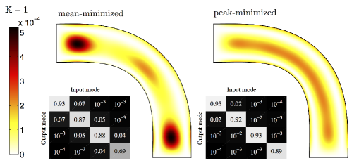
Fig. 6: Anisotropy profile and scattered-power matrices for optimized designs that minimize the mean and the peak, with $R=2.5$, $N_{\ell}=3$, and $N_{m}=6$.

4.3 Tradeoff between anisotropy and radius

In optimized structures, we found that $\max_{\mathbf{x}}\mathcal{\mathbb{K}}$ for the optimized bend, similar to the circular TO bend, decreases monotonically with $R$ (as shown in Fig. 7). Unlike the circular bend, however, this tradeoff seems asymptotically exponential rather than $\mbox{$\mathcal{O}$}(R^{-2})$. In particular, there are two clearly different regimes for this tradeoff: a power law $\mathbb{K}-1\sim R^{-4}$ at small $R\lesssim 3$ and an exponential decay $\mathbb{K}-1\sim\exp(-0.34R)$, at larger $R$. The second regime was only attained after using successive optimization, because with only one independent optimization run the algorithm tended to get stuck in local minima. For successive optimization, the optimum structure is used as a starting guess for the next run, and the initial step size is set large enough so that the algorithm can reach better local minima than the previous one.

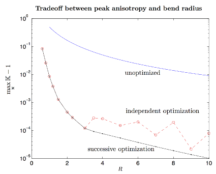
Fig. 7: Successive optimization with $N_{\ell}=5$, $N_{m}=8$ results in a power law decaying tradeoff $\max_{\mathbf{x}}\mathbb{K}-1\sim R^{-4}$ at low $R$ and an exponentially decaying tradeoff at higher $R$. For comparison, the unoptimized anisotropy for the circular TO bend is shown above.

For $R\lesssim 3$, we found that there are multiple local minima and that independent optimizations for different $R$ tend to be trapped in suboptimal local minima, as shown by the open dots in Fig. 7. To avoid this problem, we used a “successive optimization” technique in which the optimal structure for smaller $R$ is rescaled as the starting guess for local optima at a larger $R$, in order to stay along the exponential-tradeoff curve. (Another possible heuristic is “successive refinement” [131, 132, 133, 134], in which optima for smaller $N_{\ell,\,m}$ are used as starting points for optimizing using larger $N_{\ell,\,m}$.)

5 Mode squeezer

We also applied transformation inverse design to another interesting geometry: a mode squeezer that concentrates modes and their power in a small region in space, again with minimal intermodal scattering (quite unlike a conventional lens, which is intrinsically angle/mode-dependent), similar to the problem considered in [19] (which did not construct isotropic designs). We choose the untransformed region to be $-1\leq x\leq 1$ and $0\leq y\leq L$. The goal of this transformation $\mathbf{x}^{\prime}(\mathbf{x})$ is to focus the beam by minimizing the mid-beam width

$$W\equiv\intop_{-1}^{1}\mathrm{d}x\,\left.\sqrt{\left(\frac{\partial x^{\prime}}{\partial x}\right)^{2}+\left(\frac{\partial y^{\prime}}{\partial x}\right)^{2}}\right|_{y=\frac{L}{2}}.$$

As in Sec. 3.4, the transformation is written as a perturbation from the identity transformation (which was used as the starting guess) and parameterized in the spectral basis

$$x^{\prime}(x,\,y) =x+\sum_{\ell,\,m}^{N_{\ell},\,N_{m}}C_{\ell m}^{x}T_{\ell}(x)\,\sin\frac{\left(2m+1\right)\pi y}{L}$$

$$y^{\prime}(x,\,y) =y+\sum_{\ell,\,m}^{N_{\ell},\,N_{m}}C_{\ell m}^{y}T_{\ell}(x)\,\sin\frac{\left(2m+1\right)\pi y}{L},$$

The sine series automatically satisfies mirror symmetry about $y=\frac{L}{2}$ and continuity of $\mathbf{x}^{\prime}$ at the input/output interfaces $y=0,\,L$. However, we found that constraining the coefficients $C^{x,\,y}$ to enforce continuity of $\mathcal{J}$ (as in Sec. 3.4) was not necessary (although it might give a better result) since the optimization algorithm only squeezed the center region while leaving the interfaces and the regions around them relatively untouched. In this problem, we could either minimize $\mathbb{K}$ for a fixed $W$ or minimize $W$ for a fixed $\mathbb{K}$, and we happened to choose the latter.

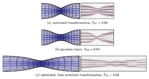
Fig. 8: Optimized squeezer outperforms gaussian taper and stretched optimized squeezers in finite element simulations.

Finite-element Maxwell simulations, shown in Fig. 8, demonstrate that the optimized design is greatly superior to a simple Gaussian taper transformation designed by hand. The Gaussian transformation was given by $x^{\prime}(\mathbf{x})=x-x\alpha\exp[-\beta(y-\frac{L}{2})^{2}]$, where $\beta>0$ and $0<\alpha<1$. Superficially, the design seems similar to an “adiabatic” taper between a wide low-index waveguide and a narrow high-index waveguide, and it is known that any sufficiently gradual taper of this form would have low scattering due to the adiabatic theorem[135]. However, the optimized TO design is much too short to be in this adiabatic regime. If it were in the adiabatic regime, then taking the same design and simply stretching the index profile to be more gradual (a taper twice as long) would reduce the scattering, but in Fig. 8 we perform precisely this experiment and find that the stretched design increases the scattering.

6 Concluding remarks

The analytical simplicity of TO design—no Maxwell equations need be solved in order to warp light in a prescribed way—paradoxically makes the application of computational techniques more attractive in order to discover the best transformation by rapidly searching a large space of possibilities. Previous work on TO design used optimization to some extent, but overconstrained the transformation by fixing the boundary shape while underconstraining the boundary conditions required for reflectionless interfaces. In fact, even our present work imposes more constraints than are strictly necessary—as long as we require continuous $\mathcal{J}$ at the input/output interfaces, there is no conceptual reason why those interfaces need be flat. A better bend, for example, might be designed by constraining the location of only two corners (to fix the bend radius) and constraining only $\mathcal{J}$ on other parts of the endfacets. However, we already achieve an exponential tradeoff between radius and anisotropy, so we suspect that further relaxing the constraints would only gain a small constant factor rather than yielding an asymptotically faster tradeoff. In the case of the mode squeezer, one could certainly achieve better results by imposing the proper $\mathcal{J}$ constraints at the endfacets. It would also be interesting to apply similar techniques to ground-plane cloaking.

All TO techniques suffer from some limitations that should be kept in mind. First, TO seems poorly suited for optical devices in which one wants to discriminate between modes (e.g. a modal filter) or to scatter light between modes (e.g. a mode transformer). TO is ideal for devices in which it is desirable that all modes be transported equally, with no scattering. Even for the latter case (such as our multimode bend), however, TO designs almost certainly trade off computational convenience for optimality, because they impose a stronger constraint than is strictly required: TO is restricted to designs where the solutions at all points in the design are coordinate transformations of the original system, whereas most devices are only concerned with the solutions at the endfacets. For example, it is conceivable that a more compact multimode bend could be designed by allowing intermodal scattering within the bend as long as the modes scatter back to their original configurations by the endfacet; the interior of the bend might not even be a waveguide, and instead might be a resonant cavity of some sort[75, 136, 76, 55]. However, optimizing over such structures seems to require solving Maxwell’s equations in some form at each optimization step, which is far more computationally expensive than the TO design and, unlike the TO design, must be repeated for different wavelengths and waveguide designs.

Appendix

In this Appendix, we briefly derive the fact, mentioned in Sec. 2.5, that the endfacet discontinuity scales much worse with anisotropy than the scalarization errors in the transformation interior, which leads us to impose an explicit continuity constraint on the Jacobian $\mathcal{J}$. In particular, we examine the Jacobian $\mathcal{J}$ for nearly isotropic transformations ($\mathbb{K}\approx 1$) that also have $\mathbf{x}^{\prime}=\mathbf{x}$ explicitly constrained at the interfaces. (The following analysis can also be straightfowardly extended to situations where $\mathbf{x}^{\prime}$ is a simple rotation of $\mathbf{x}$ on the interface, or where the interface has an arbitrary shape.) In this case, the Jacobian is

$$\mathcal{J}=\begin{pmatrix}1&0\\ \delta&1+\Delta\end{pmatrix},$$

where $\delta\equiv\frac{\partial x^{\prime}}{\partial y}$ and $\Delta\equiv\frac{\partial y^{\prime}}{\partial y}-1$ are small quantities ($\ll 1$) if $\mathcal{J}^{T}\mathcal{J}$ is nearly isotropic. The anisotropy Eq. (6) is then:

$$\mathbb{K}-1 =\frac{1+\delta^{2}+\left(1+\Delta\right)^{2}}{2\left(1+\Delta\right)}-1$$

$$=\frac{1}{2}\left(\delta^{2}+\Delta^{2}\right)+\mathcal{O}\left(\delta^{2}\Delta+\Delta^{3}\right).$$ (17)

The determinant then satisfies

$$\det\mathcal{J}-1 =\Delta$$

$$=\sqrt{2\left(\mathbb{K}-1\right)-\delta^{2}}+\mathcal{O}(\delta^{2}\Delta+\Delta^{3})$$

$$=\mathcal{O}(\sqrt{\mathbb{K}-1}).$$

This square-root dependence is also reflected in the refractive index $n^{\prime}=\sqrt{\varepsilon^{\prime}\mu^{\prime}}$ and leads to $\mathcal{O}(\mathbb{K}-1)$ power loss due to interface reflections that overwhelm the $\mathcal{O}[\left(\mathbb{K}-1\right)^{2}]$ corrections to scattered power due to the scalarization of nearly isotropic transformations (as explained in Sec. 2.5). Hence, it becomes necessary to explicitly constrain $\mathcal{J}=\mathbb{I}$ in addition to $\mathbf{x}^{\prime}=\mathbf{x}$.