A general theory of equilibrium behavior

Abstract

Economists were content with the concept of the Nash equilibrium as game theory’s solution concept until Daskalakis, Goldberg, and Papadimitriou showed that finding a Nash equilibrium is most likely a computationally hard problem, a result that set off a deep scientific crisis. Motivated, in part, by their result, in this paper, we propose a general theory of equilibrium behavior in vector fields (and, therefore, also noncooperative games). Our line of discourse is to show that these universal in nature mathematical objects are endowed with significant structure, which we probe to unearth atypical, previously unidentified, equilibrium behavior.

1 Introduction

There is evidence in the literature that various independently founded disciplines (including game theory, nonlinear optimization theory, and dynamical systems theory) have in fact been founded on variations of the same concept with the formalization of the variational inequality problem being a case in point. In the finite-dimensional variational inequality problem (for example, see [3]), we are given a set $X\subseteq\mathbb{R}^{m}$, which is typically assumed to be nonempty, closed, and convex, and a vector field $c:\mathbb{R}^{m}\rightarrow\mathbb{R}^{m}$, and our objective is to find a vector $x^{*}\in X$ such that

$$(x-x^{*})\cdot c(x^{*})\geq 0,\forall x\in X.$$

We will refer to the solutions of the variational inequality problem as the critical elements of the vector field $(X,c)$. The concept of critical elements has been shown to coincide with the concept of Nash equilibria (for example, see [15]), the concept of critical points of nonlinear optimization problems (for example, see [3]) and the concept of equilibria of dynamical systems (for example, see [8]). In this paper, we make a case toward unifying the foundations of the aforementioned disciplines by proposing a solution concept for a general vector field. The term solution concept is to be understood in the sense of game theory, namely, a prediction on the behavior of a system. First we argue that critical elements do not qualify as a solution concept for a general vector field.

1.1 Critical elements are not a solution concept

Suppose momentarily that our effort to lay a foundation of a general theory of vector fields whose objective is to make predictions through its solution concept about the behavior of systems that evolve according to vector fields is a rightful pursuit. Then we claim that critical elements cannot be that solution concept. For if critical elements qualified as such a solution concept, they would certainly need to qualify as the solutions of vector fields that have special structure, such as, for example, gradient fields, that is, vector fields that are generated by taking the gradient of a scalar function. The problem of devising a solution concept for gradient fields has been the subject of nonlinear optimization theory where it was recognized early on (in fact, by Fermat himself who formulated optimization’s first solution concepts) that critical elements are only a necessary optimality condition and by no means sufficient. (For example, consider the problem of optimizing $f(x)=x^{3}$. In this problem, $x=0$ is a critical point, that is, a solution of the aforementioned variational inequality, whereas this point does not satisfy any intuitive notion of optimality.)

In the same vein, since noncooperative games can also be represented as vector fields (for example, see [15]), does there exist solid ground to justify accepting the concept of Nash equilibrium as game theory’s solution concept? Our thesis is that it doesn’t; for one thing, computing Nash equilibria is most likely a computationally hard problem [7]. What’s more, the intersection of nonlinear optimization problems and noncooperative games is not empty: Many interesting noncooperative games are gradient fields in that they admit a potential function (for example, see [14]). Since the potential function fully characterizes the incentive structure of games that have one, on what grounds should the critical points qualify as a solution concept for these games given that critical points do not qualify to be a solution concept in the general nonlinear optimization problem?

1.2 If not critical elements, what then?

Our thesis in this paper is that the pursuit of a general theory of vector fields is rightful, and to support this thesis we propose a general theory of equilibrium behavior. The formalization of such a theory may sound at first to be a formidable and copious task considering that the concept of vector fields is as universal in mathematics as the Turing machine is in computer science, if not more. We believe, however, that our line of discourse is easy to follow as, in fact, the foundation of the theory is based on an elementary and rather intuitive idea: The elements of a vector field are comparable, and, therefore, can be ordered, in a meaningful manner. Once this idea is in place the question of devising an appropriate means by which to order them becomes a simpler (although perhaps not straightforward) task. The induced order is not, to the extent of our knowledge, a mathematical structure known prior to this work, and we take the privilege of naming it a polyorder.

1.3 The main ideas in our theory

Consider a gradient field defined over a closed and convex set $X\subseteq\mathbb{R}^{m}$ and let $f$ be its scalar potential function. Let $x,y\in X$ be arbitrary elements of this gradient field, and consider a (topological) path $p$ in $X$ starting at $x$ and ending at $y$ whose image is the convex hull of $x$ and $y$ (that is, all convex combinations of $x$ and $y$). Call $p$ a descent path if the following conditions are met: (1) $f(x)>f(y)$ and (2) $f$ is everywhere nonascending along $p$. If these conditions are met order $x$ and $y$ such that $y$ is “better than” $x$. Similarly, call $p$ a ascent path if $f(x)<f(y)$ and if $f$ is everywhere nondescending along $p$, and, if so, order $x$ and $y$ such that $x$ is “better than” $y$. A polyorder then, in this particular example of a gradient field, is the induced mathematical structure obtained by the pairwise comparison of all elements in the aforementioned way.

Now, let $x^{*}_{\min}$ be an element of $X$ such that for all other elements $x$ of $X$ the corresponding path from $x^{*}_{\min}$ to $x$ as defined above is not a descent path, and call such an element minimal; minimal elements are precisely those elements that are “no worse” than all other elements. Also, let $x^{*}_{\max}$ be an element of $X$ such that for all other elements $x$ of $X$ the corresponding path from $x^{*}_{\max}$ to $x$ is not an ascent path, and call such an element maximal; maximal elements are precisely those elements that are “no better” than all other elements.

Every polyorder has a minimum solution concept and a maximum solution concept, the former being the set of all minimal elements of $X$ and the latter being the set of all maximal elements of $X$. These ideas generalize to general vector fields, and such generalized orders form the basis of our theory of equilibrium behavior. One of the main contributions of this paper is to show how polyorders encompass various known concepts in nonlinear optimization theory and game theory and how they can evince interesting yet unidentified prior to this work behavior.

The rest of this paper is organized as follows: We motivate and formalize our theory of equilibrium behavior in the next section, while in Section 3 we explore the precise relationship between our theory and the theories of nonlinear optimization and games. Thereafter, in Section 4, we study atypical previously unknown equilibrium behavior that our theory predicts. Finally, in Section 5, we discuss related work.

2 Polytropic optimization: In search of equilibrium

In this section, we formalize our theory. We start by motivating the ideas in this theory using ideas from nonlinear optimization theory and evolutionary game theory, then we introduce some basic concepts from the theory of preference relations, and, finally, we present a precise formalization of what we may call a general theory of equilibrium behavior in vector fields.

2.1 Some motivating ideas in nonlinear programming

We start off with some basic ideas from nonlinear programming, the algorithmic component of nonlinear optimization theory. The archetypical problem of nonlinear optimization theory is to “minimize” a scalar objective function $f$ subject to a constraint set $X\subseteq\mathbb{R}^{m}$. In standard expositions of the theory, nonlinear programming algorithms would ideally compute global optima, an objective, however, that is out of the scope of existing algorithms. This observation motivates the study of algorithms with local convergence properties (for example, see [4]) and the study of optimization problems where the concepts of local and global minima coincide (for example, see [6, 5]).

Careful examination of the line of discourse of nonlinear optimization theory reveals that the concept of the objective function is not a first-order concept of this theory. Indeed, if the scope of nonlinear programming algorithms were to compute global optima, it would have been, however, as a point of fact, the objective function is only relevant inasmuch as it permits the convenient definition of descent directions.

Given a point $x$ in the constraint set $X$, a descent direction for this point is a vector in the corresponding tangent space of the constraint set such that the objective function $f$ decreases locally. What nonlinear programming algorithms essentially do is to follow descent directions in carefully selected steps and stop at points lacking descent directions. The concept of a decent direction is, therefore, arguably more important than that of the objective function.

Most texts on nonlinear optimization theory motivate the concepts of local minima and strict local minima as forming the basis of this theory’s “solution concept” in the sense that once nonlinear programming algorithms (in their course of following descent directions) arrive at such points, they stop. In this perspective, this paper can be understood as the following thought experiment: What precisely are the points that lack descent directions and do the aforementioned minimality concepts suffice to characterize these points? The precise definition of a descent direction will turn out to be crucial in this thought experiment.

2.2 Some motivating ideas in evolutionary game theory

We continue with some basic ideas from evolutionary game theory whose fundamental object of study is the population game, which is typically understood as a mathematical model of the strategic interaction among a large number of anonymous infinitesimal agents. Mathematically population games are vector fields constrained on a polyhedron that in fact generalize normal-form games.

2.2.1 Population games

A population game is a pair $(X,c)$. $X$, the game’s state space or strategy profile space, has product form, i.e., $X=X_{1}\times\cdots\times X_{n}$, where the $X_{i}$’s are simplexes and $i=1,\ldots,n$ refers to a player position (or population). To each player position corresponds a set $S_{i}$ of $m_{i}$ pure strategies and a mass $\omega_{i}>0$ (the population mass). The strategy space $X_{i}$ of player position $i$ has the form

$$X_{i}=\left\{x\in\mathbb{R}^{m_{i}}\bigg{|}\sum_{j\in S_{i}}x_{j}=\omega_{i}\right\}.$$

We refer to the elements of $X$ as states or strategy profiles. Each strategy profile $x\in X$ can be decomposed into a vector strategies, i.e., $x=(x_{1},\ldots,x_{n})^{\prime}$. Let $m=\sum_{i}m_{i}$. $c:X\rightarrow\mathbb{R}^{m}$, the game’s cost function, maps $X$, the game’s state space, to vectors of costs where each position in the vector corresponds to a pure strategy. It is typically assumed that $c$ is continuous.

2.2.2 Solution concepts for population games

Even before the result of Daskalakis et al. disputed the Nash equilibrium as game theory’s solution concept, the theory of population games was based on equilibrium refinements such as the evolutionarily stable strategy [17, 16] as well as variants and generalizations of this concept (for example, see [19]). In a manner analogous to nonlinear optimization theory, most texts on evolutionary game theory motivate the aforementioned equilibrium refinements as being this theory’s “solution concept” in the sense that they are points (or sets thereof) where evolution stops.

In contrast to nonlinear optimization theory where algorithmic ideas abound, evolutionary game theory is concerned perhaps exclusively with the concept of dynamics that although arguably would qualify as an inherently algorithmic concept from the perspective of computer scientists, it formally views evolution as a continuous-time process (with few exceptions). Evolutionarily stable strategies as well as their variants and generalizations have been shown to be attractive under a wide range of dynamics (including perhaps most prominently among them the replicator dynamic [18]). The precise definition of an evolutionarily stable strategy is based on an idea whose significance in our theory of equilibrium behavior cannot be understated.

2.2.3 The concept of invasion

One of the fundamental concepts in evolutionary game theory is that of invasion. Let $(X,c)$ be a population game, and let $x,y\in X$. We say that $x$ invades $y$ if $x\cdot c(y)<y\cdot c(y)$. The standard evolutionary interpretation of invasion is to consider a population of organisms that form a continuum mass, to interpret $y$ as the state of this population, and $y\cdot c(y)$ as the survival cost of an organism being in that state. In this vein, $x\cdot c(y)$ is the survival cost of a mutant organism whose state switches from $y$ to $x$. Then the condition that $x$ invades $y$ implies that the population of mutants will proliferate in the incumbent population due to the favorable survival cost.

There is an alternative interpretation of the concept of invasion, one that is more in alignment with ideas in nonlinear optimization theory. To that end, let’s write the condition that $x$ invades $y$ as $(x-y)\cdot c(y)<0$, and note that this implies that the angle between $c(y)$ and $(x-y)$ is obtuse. Stated differently, the projection of $c(y)$ on the line segment connecting $x$ and $y$ “points away” from $x$. Suppose now that the vector field is the gradient field of a scalar potential. Then the condition that $x$ invades $y$ is precisely the condition that $(x-y)$ is a descent direction of the scalar field at $y$ (a simple fact which is easy to prove by a Taylor expansion).

What if the vector field is not a gradient field though? Are we then justified to think of $(x-y)$ as a “descent direction” in some sense? Our intuitive understanding of a descent direction stipulates that along such a direction the objective function must decrease locally, however, as discussed earlier in the setting of nonlinear optimization theory, the objective function is not a first order concept, and, therefore, the possibility of witnessing some other more elementary phenomenon than the descent of the potential function (one that transcends to general vector fields) is open. With the benefit of hindsight, we can indeed assert that what is happening at a more elementary level is what we may call the descent of an abstract notion of an “order,” one we yet need to define. To that end, we turn to some foundational ideas from the theory of preference relations.

2.3 Some ideas in preference relations theory

Let $X$ be a nonempty set. A subset $R$ of $X\times X$ is called a binary relation on X. If $(x,y)\in R$, we write $xRy$, and if $(x,y)\not\in R$, we write $\neg xRy$. $R$ is called reflexive if $xRx$ for each $x\in X$ and complete if for each $x,y\in X$ either $xRy$ or $yRx$. It is called symmetric if, for any $x,y\in X$, we have that $xRy\Rightarrow yRx$, and antisymmetric if, for any $x,y\in X$, $xRy\wedge yRx\Rightarrow x=y$. Finally, $R$ is called transitive if for any $x,y,z\in X$ we have that $xRy$ and $yRz$ imply $xRz$.

Let $xPy\Leftrightarrow xRy\wedge\neg yRx$ and $xIy\Leftrightarrow xRy\wedge yRx$. Then $P$ and $I$ are also binary relations on X where $P\subseteq R$ and $I\subseteq R$. $P$ is called the asymmetric (or strict) part of $R$ and $I$ is called its symmetric part. If $P$ is antisymmetric, then $R$ is called a preference relation.

Preference relations are a fundamental object of study of microeconomic theory. The most elementary problem in this theory is that of individual decision making (see, for example, [10]) whose starting point is a set of alternatives (say $X$) among which an individual must choose. A fundamental tenet of microeconomic theory (since the definitive work of Von Neumann and Morgernstern [11]) is that individual preferences are rational.

Definition 1.

The preference relation $R$ is rational if it is complete and transitive.

The study of transitive preference relations is the subject of order theory (for example, see [12]); although this theory is of considerable intellectual merit, in the rest of this paper, we will be concerned with preference relations that are generally non-transitive.

If a preference relation is not transitive, one would hope that it is perhaps acyclic.

Definition 2.

The preference relation $R$ is acyclic if there is no finite set $\{x_{1},\ldots,x_{n}\}\subset X$ such that $x_{i}Rx_{i+1}$ for $i=1,\ldots,n-1$ and such that $x_{n}Rx_{1}$.

There is a growing theory of acyclic preference relations (for example, see [2, 20, 1, 13]), however, the preference relations we will be concerned with are in general not even acyclic.

Definition 3.

Let $R$ be a preference relation on $X$ and let $x,y\in X$. If $xPy$, where $P$ is the asymmetric part of $R$, we say that $x$ dominates $y$. We further say that an element of $X$ is minimal (or undominated) if there is no element in $X$ that dominates it. We, finally, say that an element of $X$ is maximal if there no element in $X$ that it dominates.

2.4 Polyorders and polytropic optimization

In the rest of this section, we introduce our solution concepts for scalar and vector fields.

2.4.1 Preliminaries

Before defining our solution concepts, however, let’s ponder momentarily why critical elements do not qualify as such. It seems intuitive to us that, in any sensible notion of optimality, points where it is possible to descend from locally should not qualify as being optimal, and it is precisely this notion of optimality that critical elements fail to pass. Consider, for example, the problem of minimizing a scalar field and an interior strict local maximum of this field. It is easy to see that the (interior) strict local maximizer is a critical element as its gradient vanishes. However, starting from the maximizer and following any direction in the tangent space, the objective function clearly does decrease, and, therefore, the maximizer cannot qualify as a solution to our minimization problem.

Our definition of an appropriate solution concept will be based on the machinery of the theory of preference relations, and, in particular, the concept of minimal or undominated elements. You may observe in the previous definition of minimality that it is a concept defined by a property that it lacks, and since we are interested in mathematically capturing the idea of points that lack descent directions, this confluence is particularly suiting. However, devising an appropriate preference ordering is not a straightforward task. To see this, recall the definition of critical elements: Given a vector field $c:X\rightarrow\mathbb{R}^{m}$, $x^{*}\in X$ is a critical element if

$$(x-x^{*})\cdot c(x^{*})\geq 0,\forall x\in X.$$

Notice in the definition that critical elements are also defined by what they lack: $x^{*}$ is a critical element precisely when it is uninvadable. Our solution concept requires a new, but straightforward in its formalism, mathematical concept, which we are going to call weak dominance in whose definition we will need the following elementary definition from topology.

Definition 4.

A path $p$ in $X\subseteq\mathbb{R}^{m}$ is a continuous map $p:[0,1]\rightarrow X$.

2.4.2 Linear scalar polyorders

Let $f:X\subseteq\mathbb{R}^{m}\rightarrow\mathbb{R}$ be a continuous scalar field where $X$ is closed and convex. Let $x,y\in X$, and define a path $y_{\epsilon}:[0,1]\rightarrow X$ such that $y_{\epsilon}=\epsilon x+(1-\epsilon)y$. Let $\preceq_{f}$ be a preference relation on $X$ such that

$$x\preceq_{f}y\Leftrightarrow\forall\epsilon_{1},\epsilon_{2}\in[0,1]:\epsilon_{1}<\epsilon_{2}\Rightarrow f(y_{\epsilon_{1}})\geq f(y_{\epsilon_{2}}).$$

If $x\preceq_{f}y$, we say that $y_{\epsilon}$ is a path of weak ascent from $x$ to $y$ (and a path of weak descent from $y$ to $x$). We call $(X,\preceq_{f})$ a linear scalar polyorder. (Note that $y_{\epsilon_{1}}$ is “closer” to $y$ than $y_{\epsilon_{2}}$.)

Proposition 1.

If $x\prec_{f}y$, then $f(x)<f(y)$.

Proof.

Since $x\prec_{f}y$, we have that $x\preceq_{f}y$ and $\neg(y\preceq_{f}x)$. Since $x\preceq_{f}y$, we have that $\forall\epsilon_{1},\epsilon_{2}\in[0,1]:\epsilon_{1}<\epsilon_{2}\Rightarrow f(y_{\epsilon_{1}})\geq f(y_{\epsilon_{2}})$. Furthermore, since $\neg(y\preceq_{f}x)$, there exist $\epsilon_{1},\epsilon_{2}\in[0,1]$, where $\epsilon_{1}<\epsilon_{2}$ such that $f(y_{\epsilon_{1}})>f(y_{\epsilon_{2}})$. Since, $f(x)\leq f(y_{\epsilon_{2}})$ and $f(y_{\epsilon_{1}})\leq f(y)$, the proof is complete. ∎

By virtue of the previous proposition, if $x\prec_{f}y$, we say that $y_{\epsilon}$ is an ascent path from $x$ to $y$ (and that $y-x$ is an ascent direction at $x$) and a descent path from $y$ to $x$ (and that $x-y$ is a descent direction at $y$). However, note that an ascent or descent direction may not be locally so in the sense that in a neighborhood of the corresponding point it may well be the case that $f$ is constant.

Proposition 2.

The strict part of a linear scalar polyorder is acyclic.

Proof.

Suppose there exists a finite set $\{x_{1},\ldots,x_{n}\}\subset X$ such that $x_{i}\prec_{f}x_{i+1}$ for $i=1,\ldots,n-1$ and such that $x_{n}\prec_{f}x_{1}$. Then $f(x_{i})<f(x_{i+1})$ for $i=1,\ldots,n-1$ and $f(x_{n})<f(x_{1})$, which contradicts the assumption that $f$ is single-valued. ∎

The previous concepts naturally generalize to general vector fields as shown next.

2.4.3 Linear vector polyorders

Let $c:X\subseteq\mathbb{R}^{m}\rightarrow\mathbb{R}^{m}$ be a continuous vector field where $X$ is closed and convex. Let $x,y\in X$, and define a path $y_{\epsilon}:[0,1]\rightarrow X$ such that $y_{\epsilon}=\epsilon x+(1-\epsilon)y$. Let $\preceq_{c}$ be a preference relation on $X$ such that

$$x\preceq_{c}y\Leftrightarrow\forall\epsilon\in[0,1]:x\cdot c(y_{\epsilon})\leq y\cdot c(y_{\epsilon}).$$

If $x\preceq_{c}y$, we say that $x$ weakly dominates $y$. We call $(X,\preceq_{c})$ a linear vector polyorder. We may understand weak dominance as follows: If $x$ weakly dominates $y$, for all $\epsilon\in[0,1]$, the projection of $c(y_{\epsilon})$ on the path $y_{\epsilon}$ does not point toward $x$.

Proposition 3.

If $x\prec_{c}y$, then $\forall\epsilon\in[0,1]:x\cdot c(y_{\epsilon})\leq y\cdot c(y_{\epsilon})$ and $\exists\epsilon\in[0,1]:x\cdot c(y_{\epsilon})<y\cdot c(y_{\epsilon})$.

Proposition 4.

The strict part of a linear vector polyorder is antisymmetric.

Proof.

The proof easily follows from the previous proposition. ∎

We now show that the concept of ‘weak dominance’ generalizes the concept of ‘weak descent’.

Proposition 5.

Let $\tilde{c}:\mathbb{R}^{m}\rightarrow\mathbb{R}^{m}$ be a continuous vector field and let $c:X\subseteq\mathbb{R}^{m}\rightarrow\mathbb{R}^{m}$ be its restriction to the closed and convex set $X$. Suppose that $\tilde{c}$ is a gradient field and let $f$ be its potential function. Then $x\preceq_{c}y\Leftrightarrow x\preceq_{f}y$.

Proof.

We show that $x\preceq_{c}y\Rightarrow x\preceq_{f}y$, noting that the reverse direction is completely analogous. To that end, let $x,y\in X$ such that $x\preceq_{c}y$, and suppose there exist $\epsilon_{1},\epsilon_{2}\in[0,1]$ where $\epsilon_{1}<\epsilon_{2}$ such that $f(y_{\epsilon_{1}})<f(y_{\epsilon_{2}})$. Then by the mean value theorem there exists $\epsilon\in(\epsilon_{1},\epsilon_{2})$ such that

$$\nabla f(y_{\epsilon})\cdot(x-y)=\frac{1}{\epsilon_{2}-\epsilon_{1}}\nabla f(y_{\epsilon})\cdot(y_{\epsilon_{2}}-y_{\epsilon_{1}})=f(y_{\epsilon_{2}})-f(y_{\epsilon_{1}})>0.$$

This contradicts our assumption that $x\preceq_{c}y$. ∎

2.4.4 Solution concepts for scalar and vector fields

What we have so far accomplished is to introduce natural, we believe, orderings of general scalar and vector fields. It is now a small step to define our solution concepts based on these orderings, definitions which we state as the following theses.

Thesis 1 (First fundamental thesis of polytropic optimization).

The minimum (resp. maximum) solution concept of a continuous scalar field that is defined over a closed and convex domain is the set of minimal (resp. maximal) elements of its linear scalar polyorder.

Thesis 2 (Second fundamental thesis of polytropic optimization).

The minimum (resp. maximum) equilibrium solution concept of a continuous vector field that is defined over a closed and convex domain is the set of minimal (resp. maximal) elements of its linear vector polyorder.

We will refer to the problem of “solving” linear scalar and vector polyorders in the sense defined above as polytropic optimization. The minimal solutions of a polytropic optimization problem are precisely those points that lack directions of descent, and it is now easy to verify that strict local maxima, for example, do not qualify as solutions of a minimization problem. Our claim, however, is much stronger: We claim that our solution concepts are a precise characterization of the intuitive notion of optimality. To support our theses, we explore, in the next section, the precise relationship between our theory and the theories of nonlinear optimization and evolutionary games.

3 Relationship with the theories of nonlinear optimization and evolutionary games

Following preliminary results, we show, in this section, that minimal and maximal elements are necessarily critical elements, and, in this sense, our solution concept is an equilibrium refinement concept. Then we show that optimization theory’s strict local minima as well evolutionary game theory’s evolutionarily stable states are minimal. Therefore, our equilibrium refinement concept encompasses the most widely applied solution concepts in these theories.

Thereafter, we explore the relationship between minimality and the concepts of local minimum and neutrally stable state. We provide examples showing that these concepts do not qualify as “solution concepts” in their respective theories and indeed they are not used as such. Our understanding from standard expositions of these theories is that local minima and neutrally stable states are equilibrium refinements that are necessary for optimality in that all optimal solutions of a nonlinear optimization problem should be local minima and that all optimal solutions of a population game should be neutrally stable. Indeed, evolutionary game theory’s most general, to the extent of our knowledge, solution concept (one that encompasses the concept of an evolutionarily stable state) is that of an evolutionarily stable set [19] (see also [21]) all of whose members are neutrally stable. Nonlinear optimization theory is not equipped with an analogue of the evolutionarily stable set, but it is easy to devise one. We prove in this section that these quite general solution concepts are encompassed in the notion of minimality, which is an intuitively pleasing result.

What’s more, we show that minimality is a more general concept than all known prior to this paper solution concepts in a strong sense: Minimal elements are not necessarily local minima. The counterexample we provide is a mathematically interesting object to which we devote Section 4.

3.1 Preliminaries: Minimal and maximal elements

In this section, we assume that $X$ is a closed and convex subset of $\mathbb{R}^{m}$, and that $c:X\rightarrow\mathbb{R}^{m}$ and $f:X\rightarrow\mathbb{R}$ are continuous.

Definition 5.

$x^{*}$ is $\preceq_{c}$-minimal if $\forall x\in X:\neg(x\prec_{c}x^{*})$. It is $\preceq_{c}$-maximal if $\forall x\in X:\neg(x^{*}\prec_{c}x)$.

The concepts of $\preceq_{f}$-minimality and $\preceq_{f}$-maximality have analogous definitions. The concepts of minimality and maximality have the following equivalent characterizations.

Lemma 1.

Let $x^{*}\in X$ and, for any $x\in X$, let $x_{\epsilon}=\epsilon x^{*}+(1-\epsilon)x$.
(i) $x^{*}$ is $\preceq_{c}$-minimal if and only if

$$\forall x:(\forall\epsilon\in[0,1]:x^{*}\cdot c(x_{\epsilon})\leq x\cdot c(x_{\epsilon}))\vee(\exists\epsilon\in[0,1]:x^{*}\cdot c(x_{\epsilon})<x\cdot c(x_{\epsilon})).$$

(ii) $x^{*}$ is $\preceq_{c}$-maximal if and only if

$$\forall x:(\forall\epsilon\in[0,1]:x^{*}\cdot c(x_{\epsilon})\geq x\cdot c(x_{\epsilon}))\vee(\exists\epsilon\in[0,1]:x^{*}\cdot c(x_{\epsilon})>x\cdot c(x_{\epsilon})).$$

(iii) $x^{*}$ is $\preceq_{f}$-minimal if and only if

$$\forall x:(\forall\epsilon_{1},\epsilon_{2}\in[0,1]:\epsilon_{1}<\epsilon_{2}\Rightarrow f(x_{\epsilon_{1}})\geq f(x_{\epsilon_{2}}))\vee(\exists\epsilon_{1},\epsilon_{2}\in[0,1]\mbox{ where }\epsilon_{1}<\epsilon_{2}:f(x_{\epsilon_{1}})>f(x_{\epsilon_{2}})).$$

(iv) $x^{*}$ is $\preceq_{f}$-maximal if and only if

$$\forall x:(\forall\epsilon_{1},\epsilon_{2}\in[0,1]:\epsilon_{1}<\epsilon_{2}\Rightarrow f(x_{\epsilon_{1}})\leq f(x_{\epsilon_{2}}))\vee(\exists\epsilon_{1},\epsilon_{2}\in[0,1]\mbox{ where }\epsilon_{1}<\epsilon_{2}:f(x_{\epsilon_{1}})<f(x_{\epsilon_{2}})).$$

Proof.

We only prove part $(i)$ as the proofs of the other parts are analogous.

$$x^{*}\mbox{ is minimal } \Leftrightarrow\forall x:\neg(x\prec x^{*})$$

$$\Leftrightarrow\forall x:\neg((x\preceq x^{*})\wedge\neg(x^{*}\preceq x))$$

$$\Leftrightarrow\forall x:(x^{*}\preceq x)\vee\neg(x\preceq x^{*})$$

$$\Leftrightarrow\forall x:(\forall\epsilon\in[0,1]:x^{*}\cdot c(x_{\epsilon})\leq x\cdot c(x_{\epsilon}))\vee\neg(\forall\epsilon\in[0,1]:x\cdot c(x^{*}_{\epsilon})\leq x^{*}\cdot c(x^{*}_{\epsilon}))$$

$$\Leftrightarrow\forall x:(\forall\epsilon\in[0,1]:x^{*}\cdot c(x_{\epsilon})\leq x\cdot c(x_{\epsilon}))\vee(\exists\epsilon\in[0,1]:x\cdot c(x^{*}_{\epsilon})>x^{*}\cdot c(x^{*}_{\epsilon}))$$

$$\Leftrightarrow\forall x:(\forall\epsilon\in[0,1]:x^{*}\cdot c(x_{\epsilon})\leq x\cdot c(x_{\epsilon}))\vee(\exists\epsilon\in[0,1]:x^{*}\cdot c(x_{\epsilon})<x\cdot c(x_{\epsilon})).\qed$$

We are going to use the following proposition.

Proposition 6.

$x^{*}$ is $\preceq_{c}$-minimal if and only if it is $\preceq_{-c}$-maximal.

Proof.

By Lemma 1, $x^{*}$ is $\preceq_{-c}$-maximal if and only if

$$\forall x:(\forall\epsilon\in[0,1]:x^{*}\cdot(-c(x_{\epsilon}))\geq x\cdot(-c(x_{\epsilon})))\vee(\exists\epsilon\in[0,1]:x^{*}\cdot(-c(x_{\epsilon}))>x\cdot(-c(x_{\epsilon}))).$$ (1)

Furthermore, by the same lemma, $x^{*}$ is $\preceq_{c}$-minimal if and only if

$$\forall x:(\forall\epsilon\in[0,1]:x^{*}\cdot c(x_{\epsilon})\leq x\cdot c(x_{\epsilon}))\vee(\exists\epsilon\in[0,1]:x^{*}\cdot c(x_{\epsilon})<x\cdot c(x_{\epsilon})).$$ (2)

But (1) and (2) are equivalent. ∎

Finally, we state without proof the following proposition.

Proposition 7.

$x^{*}$ is $\preceq_{f}$-minimal if and only if it is $\preceq_{-f}$-maximal.

3.2 Critical elements

First we show that the set of minimal elements is a subset of the set of critical elements.

Definition 6.

$x^{*}$ is a critical element of $(X,c)$ if $\forall x\in X:x\cdot c(x^{*})\geq x^{*}\cdot c(x^{*})$.

We are going to need the following lemma.

Lemma 2.

If $y\cdot c(x)<x\cdot c(x)$, then there exists $\epsilon^{\prime}\in[0,1]$ such that, $\forall\epsilon\in[\epsilon^{\prime},1]$, $y\cdot c(y_{\epsilon})<x\cdot c(y_{\epsilon})$ where $y_{\epsilon}=\epsilon x+(1-\epsilon)y$.

Proof.

The proof is a simple implication of the continuity of $(y-x)\cdot c(y_{\epsilon})$. ∎

Theorem 1.

If $x^{*}$ is $\preceq_{c}$-minimal, then $x^{*}$ is a critical element of $(X,c)$.

Proof.

Let $x^{*}$ be minimal and suppose that there exists $x\in X$ such that $x\cdot c(x^{*})<x^{*}\cdot c(x^{*})$. Then, by Lemma 2, there exists an element in the convex hull of $x^{*}$ and $x$ that dominates $x^{*}$, which contradicts our assumption that $x^{*}$ is minimal. ∎

Note that the maximal elements of $\preceq_{c}$ are, in general, not a subset of the critical elements of $(X,c)$. However, they are a subset of the critical elements of $(X,-c)$, a fact that is a simple implication of Proposition 6. Furthermore, note the following:

1. Since the maximal elements of $(X,c)$ are the minimal elements of $(X,-c)$, any theorem we prove below about minimal elements has an analogous statement for maximal elements.

2. The set of critical elements may have members that are neither minimal nor maximal. Consider, for example, $f(x)=x^{2},x\in\mathbb{R}$. Viewing $f$ as a vector field, the origin is a critical element, but it is neither a minimal nor a maximal element (since the origin is dominated by every element of the left axis and dominates every element of the right axis).

3.3 Strict local minima and evolutionarily stable states

3.3.1 Linear vector polyorders

Definition 7 (See [15]).

$x^{*}$ is an evolutionarily stable state of $(X,c)$ if there exists a neighborhood $O\subseteq X$ of $x^{*}$ such that $\forall x\in O-\{x^{*}\}:x^{*}\cdot c(x)<x\cdot c(x)$.

Theorem 2.

If $x^{*}$ is an evolutionarily stable state of $(X,c)$, then $x^{*}$ is $\preceq_{c}$-minimal.

Proof.

Let $x_{\epsilon}=\epsilon x^{*}+(1-\epsilon)x$, $\epsilon\in[0,1]$. By Lemma 1, it suffices to show that for all $x\in X$ where $x\neq x^{*}$ there exists $\epsilon\in[0,1]$ such that $x^{*}\cdot c(x_{\epsilon})<x\cdot c(x_{\epsilon})$. By the assumption that $x^{*}$ is an evolutionarily stable state, for all $x\in O$ where $x\neq x^{*}$ there exists $\epsilon\in[0,1]$ such that $x^{*}\cdot c(x_{\epsilon})<x_{\epsilon}\cdot c(x_{\epsilon})$, which is also certainly true for all $x\in X$ since $O$ is a neighborhood; expanding $x_{\epsilon}$ and rearranging proves the theorem. ∎

3.3.2 Linear scalar polyorders

Definition 8.

$x^{*}$ is a strict local minimum of $(X,f)$ if there exists a neighborhood $O\subseteq X$ of $x^{*}$ such that $\forall x\in O-\{x^{*}\}:f(x^{*})<f(x)$.

Theorem 3.

If $x^{*}$ is a strict local minimum of $(X,f)$, then $x^{*}$ is $\preceq_{f}$-minimal.

Proof.

Let $x_{\epsilon}=\epsilon x^{*}+(1-\epsilon)x$, $\epsilon\in[0,1]$. By Lemma 1, it suffices to show that for all $x\in X$ where $x\neq x^{*}$ there exist $\epsilon_{1},\epsilon_{2}\in[0,1]$ where $\epsilon_{1}<\epsilon_{2}$ such that $f(x_{\epsilon_{1}})>f(x_{\epsilon_{2}})$. Suppose, for the sake of contradiction, that this is false. Then, there exists, $x\in O$ such that $\forall\epsilon_{1},\epsilon_{2}\in[0,1]$ with $\epsilon_{1}<\epsilon_{2}$, $f(x_{\epsilon_{1}})\leq f(x_{\epsilon_{2}})$. But then $f(x)\leq f(x^{*})$, which contradicts the assumption that $x^{*}$ is a strict local minimum. ∎

3.4 Local minima, neutrally stable states, and evolutionarily stable sets

3.4.1 Linear vector polyorders

Consider the definition of a neutrally stable state in evolutionary game theory.

Definition 9.

$x^{*}$ is an neutrally stable state of $(X,c)$ if there exists a neighborhood $O\subseteq X$ of $x^{*}$ such that $\forall x\in O:x^{*}\cdot c(x)\leq x\cdot c(x)$.

We may also analogously define the concept of a local minimum of a vector polyorder.

Definition 10.

$x^{*}$ is a local minimum of $(X,\preceq_{c})$ if there exists a neighborhood $O\subseteq X$ of $x^{*}$ such that $\forall x\in O:x^{*}\preceq_{c}x$.

The concepts of local minimum of linear vector polyorders and of neutrally stable states are equivalent as the following theorem asserts.

Theorem 4.

$x^{*}$ is a neutrally stable state of $(X,c)$ $\Leftrightarrow$ $x^{*}$ is a local minimum of $(X,\preceq_{c})$.

Proof.

Let $x^{*}$ be a neutrally stable state of $(X,c)$, and let $x\in O$. Let $x_{\epsilon}=\epsilon x^{*}+(1-\epsilon)x$. Then, for all $\epsilon\in[0,1]$, we have that

$$x^{*}\cdot c(x_{\epsilon})\leq x_{\epsilon}\cdot c(x_{\epsilon}) \Leftrightarrow x^{*}\cdot c(x_{\epsilon})\leq(\epsilon x^{*}+(1-\epsilon)x)\cdot c(x_{\epsilon})$$

$$\Leftrightarrow(1-\epsilon)x^{*}\cdot c(x_{\epsilon})\leq(1-\epsilon)x\cdot c(x_{\epsilon})$$

$$\Leftrightarrow x^{*}\cdot c(x_{\epsilon})\leq x\cdot c(x_{\epsilon}),$$

and, therefore, $x^{*}\preceq_{c}x$. The reverse direction is analogous. ∎

Next we show that local minima are critical elements.

Theorem 5.

If $x^{*}$ is a local minimum of $(X,\preceq_{c})$, then $x^{*}$ is a critical element of $(X,c)$.

Proof.

Let $x^{*}$ be a local minimum of $(X,\preceq_{c})$. Then there exists $O\subseteq X$ such that $\forall x\in O\mbox{ }\forall\epsilon\in[0,1]:x^{*}\cdot c(x_{\epsilon})\leq x\cdot c(x_{\epsilon})$. Therefore, for all $x\in O$, $x\cdot c(x^{*})\geq x^{*}\cdot c(x^{*})$. Suppose now there exists $x\in X-O$ such that $x\cdot c(x^{*})<x^{*}\cdot c(x^{*})$. Then, for all $\epsilon\in[0,1]$, $x_{\epsilon}\cdot c(x^{*})<x^{*}\cdot c(x^{*})$, which contradicts the previous implication that, for all $x\in O$, $x\cdot c(x^{*})\geq x^{*}\cdot c(x^{*})$. ∎

However, as, for example, shown in Figure 1, a local minimum may not be minimal.

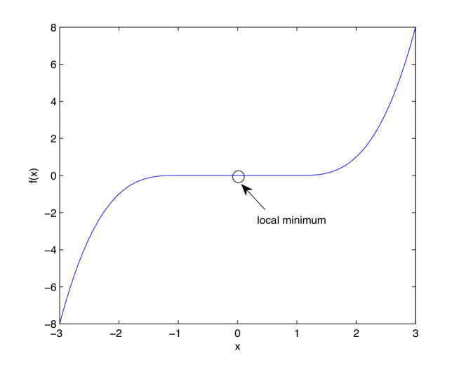
Figure 1: An example showing a local minimum element that is not minimal.

Being a local minimum is a necessary condition in a generalization of the concept of the evolutionarily stable state, namely the evolutionarily stable set.

Definition 11 (See [21]).

$X^{*}$ is an evolutionarily stable set of $(X,c)$ if it is nonempty and closed and if for each $x^{*}\in X^{*}$ there exists a neighborhood $O(x^{*})\subseteq X$ of $x^{*}$ such that $\forall x\in O(x^{*}):x^{*}\cdot c(x)\leq x\cdot c(x)$ with strict inequality if $x\not\in X^{*}$.

Evolutionarily stable sets are minimal as the following theorem asserts.

Theorem 6.

Let $X^{*}$ be an evolutionarily stable set of $(X,c)$, and let $x^{*}\in X^{*}$. Then $x^{*}$ is $\preceq_{c}$-minimal.

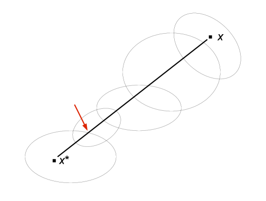
Figure 2: Used in the proof of Theorem 6.

Proof.

By Lemma 1, it suffices to show that

$$\forall x\in X:(\forall\epsilon\in[0,1]:x^{*}\cdot c(x_{\epsilon})\leq x\cdot c(x_{\epsilon}))\vee(\exists\epsilon\in[0,1]:x^{*}\cdot c(x_{\epsilon})<x\cdot c(x_{\epsilon})).$$

Note that it is trivially true (by the definition of an evolutionarily stable set) that

$$\forall x\in O(x^{*}):(\forall\epsilon\in[0,1]:x^{*}\cdot c(x_{\epsilon})\leq x\cdot c(x_{\epsilon}))\vee(\exists\epsilon\in[0,1]:x^{*}\cdot c(x_{\epsilon})<x\cdot c(x_{\epsilon})).$$

Therefore, take any $x\in X-O(x^{*})$, and let $x_{\epsilon}=\epsilon x^{*}+(1-\epsilon)x$, $\epsilon\in[0,1]$. Let $x_{\epsilon^{\prime}}$ be the point where $x_{\epsilon}$ intersects the boundary of $O(x^{*})$ (pointed at by the arrow in Figure 2), and note that to prove our claim we only need to consider the case that, for all $\epsilon\in[\epsilon^{\prime},1]$, $x^{*}\cdot c(x_{\epsilon})=x_{\epsilon^{\prime}}\cdot c(x_{\epsilon})$. Note further that in this case $x_{\epsilon^{\prime}}\in X^{*}$ and consider $O(x_{\epsilon^{\prime}})$. Let $x_{\epsilon^{\prime\prime}}$ be the point where $x_{\epsilon}$ intersects the boundary of $O(x_{\epsilon^{\prime}})$ (in the direction toward $x$). Observe now that if there exists $\zeta\in[\epsilon^{\prime},\epsilon^{\prime\prime}]$ such that $x_{\epsilon^{\prime}}\cdot c(x_{\zeta})<x_{\epsilon^{\prime\prime}}\cdot c(x_{\zeta})$, then there exists $\epsilon\in[\epsilon^{\prime},\epsilon^{\prime\prime}]$ such that $x^{*}\cdot c(x_{\epsilon})<x\cdot c(x_{\epsilon})$, and that if no such $\zeta$ exists we may similarly consider the boundary point $x_{\epsilon^{\prime\prime}}$ of $O(x_{\epsilon^{\prime}})$ noting that then, for all $\zeta\in[\epsilon^{\prime},\epsilon^{\prime\prime}]$, $x_{\epsilon^{\prime}}\cdot c(x_{\zeta})=x_{\epsilon^{\prime\prime}}\cdot c(x_{\zeta})$, and, therefore, that $x_{\epsilon^{\prime\prime}}\in X^{*}$. Continuing in this way, we either obtain an $\epsilon\in[0,1]$ such that $x^{*}\cdot c(x_{\epsilon})<x\cdot c(x_{\epsilon})$ or we have that, for all $\epsilon\in[0,1]$, $x^{*}\cdot c(x_{\epsilon})=x\cdot c(x_{\epsilon})$. Since $x$ is arbitrary, the theorem is proven. ∎

3.4.2 Linear scalar polyorders

In the last part of this section, we explore the analogue of the concept of the evolutionarily stable set in scalar fields. To that end, consider the definition of a local minimum in nonlinear optimization.

Definition 12.

$x^{*}$ is a local minimum of $(X,f)$ if there exists a neighborhood $O\subseteq X$ of $x^{*}$ such that $\forall x\in O:f(x^{*})\leq f(x)$.

We may also analogously define the concept of a local minimum of a scalar polyorder.

Definition 13.

$x^{*}$ is a local minimum of $(X,\preceq_{f})$ if there exists a neighborhood $O\subseteq X$ of $x^{*}$ such that $\forall x\in O:x^{*}\preceq_{f}x$.

We have the following theorem.

Theorem 7.

If $x^{*}$ is a local minimum of $(X,\preceq_{f})$, then $x^{*}$ is a local minimum of $(X,f)$.

Proof.

Since $x^{*}$ is a local minimum of $(X,\preceq_{f})$, for all $x\in O$, we have that, for all $\epsilon_{1},\epsilon_{2}\in[0,1]$ where $\epsilon_{1}<\epsilon_{2}$, $f(x_{\epsilon_{1}})\geq f(x_{\epsilon_{2}})$, which is certainly true if $\epsilon_{1}=0$ and $\epsilon_{2}=1$. ∎

However, the reverse direction is not generally true. For example, consider a scalar field $f:\mathbb{R}^{2}\rightarrow\mathbb{R}$ that is obtained by rotating the function in Figure 3 around the $z$-axis (the figure shows the intersection of such a function with the plane $y=0$). It is easy to see in this example that the global minima of $f$ are not local minima of $\preceq_{f}$. (To see this note that the global minima of $f$ form a circle and take any two points on this circle.)

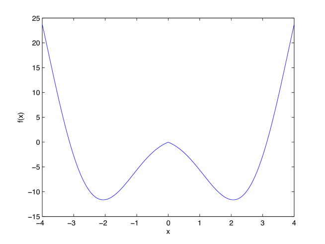
Figure 3: Rotating this function around the vertical axis (at $x=0$) we obtain a scalar field whose global minima are not local minima of $\preceq_{f}$.

Since the local minima of a scalar field are not necessarily local minima of its corresponding scalar polyorder, we are motivated to strengthen the definition of an evolutionarily stable set in scalar fields by introducing a new concept, namely that of an almost strictly minimal set.

Definition 14.

$X^{*}$ is an almost strictly minimal set of $(X,f)$ if it is nonempty and closed and if for each $x^{*}\in X^{*}$ there exists a neighborhood $O(x^{*})\subseteq X$ of $x^{*}$ such that $\forall x\in O(x^{*}):f(x^{*})\leq f(x)$ with strict inequality if $x\not\in X^{*}$.

We have the following theorem, which is a stronger form of Theorem 6.

Theorem 8.

Let $X^{*}$ be an almost strictly minimal set of $(X,c)$, and let $x^{*}\in X^{*}$. Then $x^{*}$ is $\preceq_{f}$-minimal.

Proof.

The proof is analogous to that of Theorem 6, however, it is worth noticing the subtle differences in the beginning of the proof. By Lemma 1, it suffices to show that

$$\forall x:(\forall\epsilon_{1},\epsilon_{2}\in[0,1]:\epsilon_{1}<\epsilon_{2}\Rightarrow f(x_{\epsilon_{1}})\geq f(x_{\epsilon_{2}}))\vee(\exists\epsilon_{1},\epsilon_{2}\in[0,1]\mbox{ where }\epsilon_{1}<\epsilon_{2}:f(x_{\epsilon_{1}})>f(x_{\epsilon_{2}})).$$

It is easy to show that the previous statement is true for all $x\in O(x^{*})$. (The negation of the previous statement implies there exists a descent path starting at $x^{*}$, which contradicts the assumption that $x^{*}$ is a local minimum.) Therefore, let $x\in X-O(x^{*})$, and let $x_{\epsilon}=\epsilon x^{*}+(1-\epsilon)x$, $\epsilon\in[0,1]$. Let $x_{\epsilon^{\prime}}$ be the point where $x_{\epsilon}$ intersects the boundary of $O(x^{*})$, and note that to prove our claim we only need to consider the case that, for all $\epsilon_{1},\epsilon_{2}\in[\epsilon^{\prime},1]$ with $\epsilon_{1}<\epsilon_{2}$ we have that $f(x_{\epsilon_{1}})\geq f(x_{\epsilon_{2}})$, in which case $f(x^{*})=f(x_{\epsilon^{\prime}})$ and, therefore, $x_{\epsilon^{\prime}}\in X^{*}$. From this point on the proof is completely analogous to that of Theorem 6. ∎

The converse of the previous theorem does not hold in general and, therefore, the concept of almost strict minimality does not characterize the concept of minimality. The next section is devoted to studying such a counterexample.

4 Atypical solutions of polytropic optimization

In this section, we study an optimization problem whose solution has atypical structure. The problem is that of optimizing $f(x)=x\sin(1/x),x\in\mathbb{R}$ (shown in Figure 4). Note that $f$ is differentiable everywhere except the origin where it is continuous. Note also that the solution of the scalar polyorder of $f$ is different from the solution of its vector polyorder, although both solutions have similar structure.

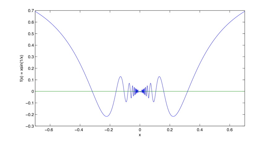
Figure 4: The graph of $f(x)=x\sin(1/x)$.

What is peculiar about the problem of optimizing $f$ is that the critical element $x=0$ is both minimal and maximal (in both polyorders) without being a local minimum or a local maximum (in either polyorder), however, it satisfies our definition of optimality because there exists neither a descent nor an ascent path on either side.

In spite of the origin’s atypical behavior, the optimal solutions of $f$ have a particularly attractive property once we view them as a set, namely, they are “setwise locally dominant” in that there exists a neighborhood of the set of minimal elements such that every element in this neighborhood is either minimal or it is dominated by a minimal element.

We also consider the dynamical system $dx/dt=-f(x)$. Looked at from a dynamical systems perspective, the origin is similarly peculiar: For one thing, it is neither an isolated point of the set of critical elements, as any neighborhood contains infinitely many critical elements, nor an interior point of that set. What’s more, to approach the origin starting at any $x_{0}\neq 0$ a physical system navigating $f$ has to “reverse” its evolution rule an infinite number of times, and on the grounds of this observation, we may, therefore, informally say that the origin would practically be “spaced out” for most physical systems. However, we show that the set of minimal elements is asymptotically stable as a set.

4.1 Optimal solutions of $x\sin(1/x)$

Lemma 3.

Let $f:\mathbb{R}\rightarrow\mathbb{R}$ be continuous, let $x^{*}$ be an isolated critical point of $f$, and suppose $f$ is differentiable in a neighborhood of $x^{*}$. Then, if $f^{\prime}(x^{*})>0$, $x^{*}$ is minimal, whereas if $f^{\prime}(x^{*})<0$, $x^{*}$ is maximal.

Proof.

Suppose $f^{\prime}(x^{*})>0$. It suffices to show, for all $x\in\mathbb{R}-\{x^{*}\}$, there exists $\epsilon\in[0,1]$ such that $x^{*}f(x_{\epsilon})<xf(x_{\epsilon})$. Expanding $f$ around $x^{*}$ we have that $f(x_{\epsilon})=f^{\prime}(x^{*})(x_{\epsilon}-x^{*})+o(|x_{\epsilon}-x^{*}|^{2})$ and, therefore, that $(x^{*}-x)f(x_{\epsilon})=(1/1-\epsilon)(x^{*}-x_{\epsilon})f(x_{\epsilon})\approx-(1/1-\epsilon)(x^{*}-x_{\epsilon})^{2}f^{\prime}(x^{*})<0$ in a neighborhood of $x^{*}$. The proof that $x^{*}$ is maximal if $f^{\prime}(x^{*})<0$ is analogous. ∎

Theorem 9.

Viewing $f(x)=x\sin(1/x)$ as a vector field, the set of its minimal elements is

$$X^{*}_{\min}=\{1/n\pi|n=1,3,5,\ldots\}\cup\{0\}\cup\{1/n\pi|n=-2,-4,-6,\ldots\},$$

and the set of its maximal elements is

$$X^{*}_{\max}=\{1/n\pi|n=2,4,6,\ldots\}\cup\{0\}\cup\{1/n\pi|n=-1,-3,-5,\ldots\}.$$

Proof.

The critical points of $f$ are $\{0\}\cup\{1/n\pi|n=\pm 1,\pm 2,\pm 3,\ldots\}$. Note now that every critical point except the origin is an isolated point and that $f$ is differentiable everywhere except at $0$. Therefore, we may use Lemma 3 to characterize all critical points except the origin. To show that the elements of $X^{*}_{\min}-\{0\}$ are minimal and that the elements of $X^{*}_{\max}-\{0\}$ are maximal is then a matter of simple calculus. Consider now the origin. To show that the origin is both minimal and maximal it suffices to show that, for all $x\in\mathbb{R}-\{0\}$, there exists $\epsilon\in[0,1]$ such that $0<xf(x_{\epsilon})\Leftrightarrow\sin(1/x_{\epsilon})>0$ and $\epsilon^{\prime}\in[0,1]$ such that $0>xf(x_{\epsilon^{\prime}})\Leftrightarrow\sin(1/x_{\epsilon^{\prime}})<0$. Both properties follow by elementary properties of the sinusoidal function. ∎

4.2 Minimal elements are setwise locally dominant

Proposition 8.

Every non-minimal element of the interval $[-1/\pi,+\infty)$ is dominated by a minimal element.

Proof.

First we show that the “rightmost” minimal element, that is, minimal element $x^{*}=1/\pi$, dominates every element in the interval $(1/\pi,+\infty)$. Letting $x\in(1/\pi,+\infty)$, it suffices to show that $(x^{*}-x)f(x)<0$, which holds since $x^{*}<x$ and $f(x)>0$. Next we show that the same minimal element dominates every element in the interval $(1/2\pi,1/\pi)$. Letting $x\in(1/2\pi,1/\pi)$, it suffices to show that $(x^{*}-x)f(x)<0$, which holds since $x^{*}>x$ and $f(x)<0$. Now we show that the minimal element $x^{*}=1/(2k+1)\pi,k=1,2,3,\ldots$ dominates every element in the intervals $(1/(2k+1)\pi,1/2k\pi)$ and $(1/2(k+1)\pi,1/(2k+1)\pi)$. Again it is suffices to show that $(x^{*}-x)f(x)<0$ where $x$ is any element in one of those intervals. If $x\in(1/(2k+1)\pi,1/2k\pi)$, then $x^{*}<x$ and $f(x)>0$ (to see this note that since $x^{*}$ is minimal $f^{\prime}(x^{*})>0$) whereas if $x\in(1/2(k+1)\pi,1/(2k+1)\pi)$ then $x^{*}>x$ and $f(x)<0$. Therefore, every element on the right halfline is either minimal or it is dominated by a minimal element. The proof for the left halfline is similar, noting that $x^{*}=-1/\pi$ is maximal, and, therefore, it is dominated by every element in the interval $(-\infty,-1/\pi)$. ∎

4.3 Minimal elements are setwise asymptotically stable

4.3.1 Preliminaries

Following [9], consider the differential equation

$$\dot{x}=F(x)$$ (3)

where $F:X\subseteq\mathbb{R}^{m}\rightarrow\mathbb{R}^{m}$ and $X$ is open in $\mathbb{R}^{m}$. Let $x^{*}$ be an equilibrium of this equation (that is, an element of $X$ such that $F(x^{*})=0$). We call $x^{*}$ a stable equilibrium if for every neighborhood $O\subseteq X$ of $x^{*}$ there is a neighborhood $O^{\prime}\subseteq X$ of $x^{*}$ such that every solution $x(t)$ with $x(0)\in O$ is defined and is in $O^{\prime}$ for all $t>0$. If $O^{\prime}$ can be chosen so that in addition to the previous property, $\lim_{t\rightarrow+\infty}x(t)=x^{*}$, then $x^{*}$ is asymptotically stable.

Theorem 10 (See [9]).

Let $x^{*}$ be an equilibrium of (3). Let $L:O\rightarrow\mathbb{R}$ be continuous function defined on a neighborhood $O\subseteq X$ of $x^{*}$, differentiable on $O-x^{*}$, such that $L(x^{*})=0$, $L(x)>0$ if $x\neq x^{*}$, and $\dot{L}\leq 0$ in $O-x^{*}$. Then $x^{*}$ is stable. If also $\dot{L}<0$ in $O-x^{*}$, then $x^{*}$ is asymptotically stable.

Following [15], let $X^{*}\subseteq X$ be a closed set, and call $O\subseteq X$ a neighborhood of $X^{*}$ if it open relative to $X$ and contains $X^{*}$. Call $X^{*}$ Lyapunov stable under (3) if for every neighborhood $O$ of $X^{*}$ there exists a neighborhood $O^{\prime}$ of $X^{*}$ such that every solution $\{x_{t}\}$ that start in $O^{\prime}$ is contained in $O$: that is, $x_{0}\in O^{\prime}$ implies that $x_{t}\in O$ for all $t\geq 0$. $X^{*}$ is attracting if there is a neighborhood $\mathcal{O}$ of $X^{*}$ such that every solution that starts in $\mathcal{O}$ converges to $X^{*}$: that is, $x_{0}\in\mathcal{O}$ implies that $\omega(\{x_{t}\})\subseteq X^{*}$. $X^{*}$ is globally attracting if it is attracting with $\mathcal{O}=X$. Finally, the set $X^{*}$ is asymptotically stable if it is Lyapunov stable and attracting, and it is globally asymptotically stable if it is Lyapynov stable and globally attracting.

Theorem 11 (See [15]).

Let $X^{*}\subseteq X$ be closed, and let $\mathcal{O}\subseteq X$ be a neighborhood of $X^{*}$. Let $L:\mathcal{O}\rightarrow\mathbb{R}_{+}$ be $C^{1}$ with $L^{-1}(0)=X^{*}$. If $\dot{L}(x)\equiv\nabla L(x)^{\prime}F(x)<0$ for all $\mathcal{O}-X^{*}$, the $X^{*}$ is asymptotically stable under (3). If in addition $\mathcal{O}=X$, then $X^{*}$ is globally asymptotically stable under (3).

4.3.2 Minimal elements are setwise asymptotically stable

Theorem 12.

$X^{*}_{\min}$, the set of minimal elements of $f(x)=x\sin(1/x),x\in\mathbb{R}$, is asymptotically stable under $\dot{x}=-x\sin(1/x)$.

In the proof of this theorem we are going to need the following lemma.

Lemma 4.

Let $\dot{x}=-f(x)$. Then we have:
(i) $1/\pi$ is globally asymptotically stable in $(1/2\pi,+\infty)$.
(ii) $1/(2k+1)\pi,k=1,2,\ldots$ is globally asymptotically stable in $(1/2k\pi,1/2(k+1)\pi)$.
(iii) $-1/2k\pi,k=1,2,\ldots$ is globally asymptotically stable in $(-1/(2k-1)\pi,-1/(2k+1)\pi)$.

Proof.

To prove part (i), let $L_{1/\pi}(x)=\int_{1/\pi}^{x}f(y)dy$. Then $L(1/\pi)=0$, $L^{\prime}(x)=f(x)$, and $\dot{L}(x)=-f^{2}(x)$. Therefore, $\dot{L}(x)<0,x\neq 1/\pi$, which proves part (i). The proof of part (ii) is derived using a similar line of reasoning using $L_{1/(2k+1)\pi}(x)=\int_{1/(2k+1)\pi}^{x}f(y)dy$ and likewise for part (iii). ∎

Proof of Theorem 12.

Since, by Lemma 4, every solution that starts in $(-1/\pi,+\infty)$ remains in this set, $X^{*}_{\min}$ is Lyapunov stable. What’s more, by the same lemma, every solution that starts in $(-1/\pi,+\infty)$ converges to $X^{*}_{\min}$. Therefore, $X^{*}_{\min}$ is asymptotically stable. ∎

5 Related work

To the extent of our knowledge, this is the first paper that proposes a general theory of equilibrium behavior in vector fields. Our theory builds upon various related ideas in the literature perhaps the most significant of which are the formalization of the variational inequality problem, the concept of invasion in evolutionary game theory and the concept of descent algorithms in nonlinear optimization theory, and last but not least order theory. It is difficult to trace the origins and evolution of these ideas in one paper (for example, optimization theory’s necessary optimality conditions date as far back as 1637; see [4]), and we defer from providing definitive references.

5.1 The variational inequality problem

The variational inequality problem captures the notion of equilibrium in its generality and represents, in our view, the first attempt to formalize a general theory of equilibrium behavior. However, our theory refines the concept of variational equilibrium in a strong sense. According to their variational formalization, equilibria are precisely those points that lack (a generalized notion of) directions of strict descent. In contrast, minimal elements are precisely those points that lack (a generalized notion of) directions of descent. Since points that lack directions of descent clearly lack directions of strict descent, minimal elements are a variational equilibrium refinement concept. Therefore, the concept of variational equilibrium is a necessary condition in any fixed (equilibrium) solution of a vector field, however, we have argued extensively that this concept cannot serve as a general solution concept in vector fields.

5.2 Nonlinear optimization theory and game theory

One of the main contributions of this paper is to explore the precise relationship between evolutionary game theory and nonlinear optimization theory: Drawing on the link that the variational inequality problem establishes between the equilibrium concepts of these theories, this is the first paper to establish a relationship between the evolutionarily stable state and the strict local minimum. However, our contribution extends beyond establishing this relationship to extending both theories through proposing an overarching solution concept (of which both the evolutionarily stable state and the strict local minimum are special cases).

At a more elementary conceptual level, we believe that evolutionary game theory’s most significant contribution in the study of equilibrium behavior is the concept of evolutionary stability, and although there are many alternative formalizations of this concept, they have been shown to be equivalent. These formalizations are all based on the more elementary concept of invasion. Our theory is based instead on the elementary concept of dominance, which furnishes a solution concept that generalizes the concept of evolutionary stability in a strong sense.

Similarly, nonlinear optimization theory’s formalizations are based on the elementary concept of a direction of strict descent whereas our theory is based instead on the concept of a descent path (that is germane to the concept of dominance). This change in perspective furnishes a solution concept that generalizes nonlinear optimization theory’s solution concepts.

5.3 Order theory

The concept of a polyorder draws heavily on ideas from order theory, a discipline which is concerned, however, with the study of transitive binary relations (see, for example, [12]), whereas polyorders are generally not transitive. As discussed earlier, there is an increasing body of work on acyclic binary relations, a concept that relaxes the concept of transitivity. Although scalar polyorders are acyclic (Proposition 2), the rich structure of scalar polyorders warrants independent scrutiny.

References

- [1] J. C. R. Alcantud. Characterization of the existence of maximal elements of acyclic relations. Economic Theory, 19:407–416, 2002.
- [2] T. Bergstrom. Maximal elements of acyclic relations on compact sets. Journal of Economic Theory, 10:403–404, 1975.
- [3] D. Bertsekas and J. Tsitsiklis. Parallel and Distributed Computation: Numerical Methods. Prentice Hall, 1989.
- [4] D. P. Bertsekas. Nonlinear Programming. Athena Scientific, second edition, 1999.
- [5] D. P. Bertsekas, A. Nedic, and A. E. Ozdaglar. Convex Analysis and Optimization. Athena Scientific, 2003.
- [6] S. Boyd and L. Vandenberghe. Convex Optimization. Cambridge University Press, 2004.
- [7] C. Daskalakis, P. W. Goldberg, and C. H. Papadimitriou. The complexity of computing a Nash equilibrium. SIAM J. Comput., 39(1):195–259, 2009.
- [8] P. Dupuis and A. Nagurney. Dynamical systems and variational inequalities. Annals of Operations Research, 44:9–42, 1993.
- [9] M. W. Hirsch and S. Smale. Differential Equations, Dynamical Systems, and Linear Algebra. Academic Press, 1974.
- [10] A. Mas-Colell, M. D. Whinston, and J. R. Green. Microeconomic Theory. Oxford University Press, 1995.
- [11] J. Von Neumann and O. Morgernstern. Theory of Games and Economic Behavior. Princeton University Press, 1953.
- [12] E. A. Ok. Elements of Order Theory, 2012. https://files.nyu.edu/eo1/public/books.html.
- [13] H. Salonen and H. Vartiainen. On the existence of undominated elements of acyclic relations. Mathematical Social Sciences, 60:217–221, 2010.
- [14] W. Sandholm. Potential games with continuous player sets. Journal of Economic Theory, 97:81–108, 2001.
- [15] W. H. Sandholm. Population Games and Evolutionary Dynamics. MIT Press, 2010.
- [16] J. Maynard Smith. Evolution and the Theory of Games. Cambridge University Press, 1982.
- [17] J. Maynard Smith and G. R. Price. The logic of animal conflict. Nature, 246:15–18, 1973.
- [18] P. Taylor and L. Jonker. Evolutionary stable strategies and game dynamics. Mathematical Biosciences, 16:76–83, 1978.
- [19] B. Thomas. On evolutionarily stable sets. J. Math. Biology, 22:105–115, 1985.
- [20] M. Walker. On the existence of maximal elements. Journal of Economic Theory, 16:470–474, 1977.
- [21] J. W. Weibull. Evolutionary Game Theory. MIT Press, 1995.