xrayutilities: A versatile tool for reciprocal space conversion of scattering data recorded with linear and area detectors

Abstract

We present general algorithms to convert scattering data of linear and area detectors recorded in various scattering geometries to reciprocal space coordinates. The presented algorithms work for any goniometer configuration including popular four-circle, six-circle and kappa goniometers. We avoid the use of commonly employed approximations and therefore provide algorithms which work also for large detectors at small sample detector distances. A recipe for determining the necessary detector parameters including mostly ignored misalignments is given. The algorithms are implemented in a freely available open-source package.

Algorithms for the reciprocal space conversion of linear and area detectors implemented in an open-source Python package.

1 Introduction

Elastic X-ray scattering is a very widely applied technique to study the structure of materials ranging from single crystals, powders and other forms of hard condensed matter to biologic tissues and organic molecules. Crystalline as well as non-crystalline matter like liquids and amorphous materials can be studied by techniques like X-ray diffraction and reflectometry. A variety of approaches exist to analyze the scattering data. Some quantities can be directly determined from the measurements (e. g. lattice parameters [Bond1960, Fewster1999], layer thicknesses [Warren1969, Pietsch2004]). Other types of analysis involve simulation of the scattering signal to determine strain and material composition [Stangl2004, Wintersberger2010], or the model-free determination of real space structure using phase retrieval algorithms [Fienup1982, Miao1998, Diaz2009, Minkevich2011]. All of those approaches have in common that the analysis is most of the time performed in reciprocal space, and hence require a conversion of experimentally measured data into reciprocal space. While the particular analysis steps differ for different experiments, the conversion itself is a common step, which needs to be performed for a lot of different techniques. This has been treated very well for the case of point detectors [Busing1967, Lohmeier1993, You1999, Bunk2004]. For 1D and 2D detectors, which are used more and more frequently, several issues related to the detector geometry and detector alignment complicate a correct conversion.

For some application like protein crystallography or powder diffraction, experimental as well as analysis schemes are standardized. Examples are software packages to extract peak positions and intensities in protein-crystallography[Leslie2006] and powder diffraction [Lutterotti1999, Rodriguez2001, fit2d], or the pdb protein data bank format and cif crystallographic information file format established by the International Union of Crystallography for exchange of structure files and experimental data.

For most other cases, only very specialized solutions to particular experiments exist, each containing solutions for some aspects important for the respective case, e. g. the experimental control software spec [certif] used at various synchrotron sources is able to do reciprocal space conversion for several goniometer geometries, however only for point detectors. Commercial software supplied with several diffractometers is optimized for certain geometry/detector combinations.

A particular problem of 1D and 2D detectors are misalignments with respect to the ideal case: At zero detector angle, the line or plane of the detector should ideally be perpendicular to the incident X-ray beam. In practice, this will not be the case, even if deviations will usually be very small. For 2D-detectors, in addition a rotation of the detector around the incident beam direction can occur. In most cases, these misalignments will be unintentional and rather small, they are difficult to measure and hence often neglected. However, considering these effects is actually important to obtain correct and accurate reciprocal space coordinates.

We present a general applicable algorithm for the conversion of experimental data recorded with point, linear and area detectors, and for any diffractometer with arbitrary number and sequence of axes. For this purpose, we generalize the algorithms presented in several papers [Busing1967, Lohmeier1993, You1999, Bunk2004] to arbitrary goniometer geometries without approximations: we consider the fact that most 1D and 2D detectors are flat and hence the relation between channel number and scattering angle is non-linear. Furthermore, we provide recipes how to determine the necessary detector parameters from a set of simple scans around the primary beam. These scans also enable the user to determine the mentioned and several other misalignment parameters.

To keep our solution as general as possible, we have implemented it within a freely available software package xrayutilities [xrutils_web]. This generalized algorithm is also particularly useful for automatized tool-chains as planned by several synchrotron facilities right now [passerelle]. In addition to the reciprocal space conversion described in this article, xrayutilities includes routines to read various data formats and methods to calculate experimental parameters from material properties. More information on those parts can be found on the xrayutilities web page [xrutils_web]. This article focuses on the reciprocal space conversion part: After the introduction of the applied algorithms following the approach of You, 1999 we show the extension for linear and area detectors and explain the use of our algorithms and how necessary parameters can be determined. We demonstrate the application of our approach for few selected examples of both laboratory diffractometers and synchrotron beamlines. In the appendix we discuss one complete example, including the particular entries into the xrayutilities package to define the diffractometer geometry, correctly initialize a 2D detector setup, and convert a 2D detector frame into reciprocal space.

2 Angular to reciprocal space conversion

Conversion of angular coordinates to reciprocal space can be tedious since one needs special equations for every diffractometer/detector geometry. For several diffraction geometries explicit formulas are given for example in Pietsch, 2004. However the conversion can be performed in a general way as long as the information about the goniometer geometry is available together with the experimental angles. The algorithm presented below therefore needs not just the experimental angles as input parameters but also the description of the goniometer. To work for arbitrary goniometers the physical order of the cradles, i. e. how they are mounted on each other, as well as the orientation of the rotation axes are needed. An example is given below. To unambiguously specify the rotation axes of the goniometer circles, a reference coordinate system is fixed to the laboratory frame. It is useful to choose this coordinate system in a way that the primary X-ray beam propagates along one of the coordinate axes.

The reciprocal space coordinates we want to know for each measured point are coordinates of the momentum transfer $\boldsymbol{q}=\boldsymbol{k}_{f}-\boldsymbol{k}_{i}$, where $\boldsymbol{k}_{i}$ is the wave-vector of the incident X-ray beam, $\boldsymbol{k}_{f}$ the wave-vector of the scattered beam towards a particular detector (pixel) position. The coordinates of $\boldsymbol{q}$ we are interested in are those in a coordinate system fixed to the sample under investigation. The coordinates of $\boldsymbol{k}_{i}$ in the laboratory system are fixed by our choice of the coordinate system. The coordinates of $\boldsymbol{k}_{f}$ are given by the angle positions of the detector arm. To describe $\boldsymbol{q}$ in the sample coordinate system, we also need all goniometer angles changing the sample orientation.

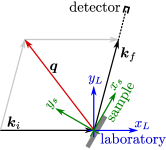
Figure 1: Two dimensional sketch of the scattering process and the coordinate systems attached to the laboratory ($x_{L}$,$y_{L}$) and sample ($x_{s}$,$y_{s}$). Shown are the incidence and exit wave vectors $\boldsymbol{k}_{i,f}$ as well as the momentum transfer of the scattering process $\boldsymbol{q}$. The laboratory coordinate system is chosen to have the $\boldsymbol{\hat{x}}$ direction to coincide with the primary beam direction.

A minimal two dimensional example illustrating the definition of our laboratory coordinate system (blue) is shown in Fig. 1. The coordinate system attached to the sample is indicated in green in Fig. 1. So what we have to deal with are coordinate transformations between the different involved coordinate systems. Those coordinate transformations can be written as matrix equations. We will reproduce some of the essential equations of earlier papers [Busing1967, You1999] so that reader can follow the further generalization for one and two dimensional detectors. We consider just a point detector for the moment, the generalization for one or two dimensional detectors is shown in Sec. 3 below.

The sample coordinate system we have been talking about is actually the coordinate system attached to the innermost goniometer circle (because this is what the goniometer angles describe). Of course, the sample can in addition have a certain orientation with respect to this circle. This is most evident in the case of a crystalline sample, where the directions of the reciprocal space of the crystal have a certain orientation with respect to the sample holder. This and the coordinates of the momentum transfer in the reciprocal space of the crystal are described below by matrices $\uuline{U}$ and $\uuline{B}$, respectively. In the following, we describe this ”most complicated” case of a single crystalline sample. For amorphous or powder samples etc., $\uuline{U}$ and/or $\uuline{B}$ can be replaced by identity matrices.

In the crystal lattice a momentum transfer might be described by the column vector

$$\boldsymbol{h}_{c}=\sum_{j=1}^{3}h_{j}\boldsymbol{b}_{j}=\uuline{B}\boldsymbol{h}$$ (1)

with $\boldsymbol{b}_{j}$ the reciprocal lattice vectors or the matrix $\uuline{B}$ formed from those vectors and $h_{j}$ generally referred to as $h$, $k$, $l$. In case $h$, $k$, $l$ are integer values they are called Miller indices. An explicit representation of $\uuline{B}$ is for example given in [Busing1967].

To connect the momentum transfer in the crystal with the momentum transfer in the coordinate system attached to the sample goniometer the orientation matrix $\uuline{U}$ is introduced.

$$\boldsymbol{h}_{s}=\uuline{U}\boldsymbol{h}_{c}=\uuline{U}\,\uuline{B}\boldsymbol{h}$$ (2)

This momentum transfer converted to the laboratory frame is equal to $\boldsymbol{q}$. The conversion of the momentum transfer is achieved by another coordinate transformation (described by matrix $\uuline{S}$), which solely depends on the sample orientation and therefore the goniometer angles which move the sample.

$$\boldsymbol{q}=\boldsymbol{k}_{f}-\boldsymbol{k}_{i}=\uuline{S}\boldsymbol{h}_{s}$$ (3)

In the case of integer $h$, $k$, $l$, the former equation basically is the Laue equation.

Also any detector rotation can be expressed as coordinate transformation described by $\uuline{D}$ and therefore the exit wave vector is given by

$$\boldsymbol{k}_{f}=\uuline{D}\boldsymbol{k}_{i}$$ (4)

Combining Eqs. 2 to 4 one obtains the momentum transfer in the crystal coordinate system

$$\boldsymbol{h}_{c}=\left(\uuline{S}\,\uuline{U}\right)^{-1}\left(\uuline{D}-\uuline{1}\right)\boldsymbol{k}_{i}$$ (5)

with the identity matrix $\uuline{1}$. Note that all of the used coordinate transformations are transformations between two orthogonal coordinate systems, and therefore yield orthogonal matrices, which are invertible. The matrix $\uuline{B}$, which is formed from the reciprocal space vectors $\boldsymbol{b}_{j}$, which are linear independent is also invertible. Since the above conversion involves a matrix inversion this is important for the algorithm to work.

The rotation matrices $\uuline{S}$ and $\uuline{D}$ can be deduced from the description of the goniometer by multiplying the rotation matrices from each circle starting with the outer most circle.

$$\uuline{D},\uuline{S}=\text{(outer most)}\cdot\dots\cdot\text{(inner most)}$$ (6)

For that purpose the goniometer rotation axis needs to be defined in the laboratory coordinate system for the case when all circles are set to zero. It is therefore useful to choose the coordinate system in a way, which allows this description to be as simple as possible. Keep in mind that later also the detector directions need to be determined in this coordinate system. In addition to the direction of the rotation axis also the rotation sense needs to be described. We use the mathematical definition of rotation sense. For most goniometers (except for special geometries like $\kappa$-goniometer, treated separately below) the rotation axis point along primitive directions. When looking on the rotation from the positive side of the corresponding direction, clockwise rotation is left-handed, i. e., negative, and an anticlockwise rotation is right-handed (positive). For example, we will call a clockwise/left-handed/negative rotation of angle $\alpha$ around the $x$-axis a ’x-’-rotation, described by the following rotation matrix:

$$\uuline{R}_{x-}(\alpha)=\begin{pmatrix}1&0&0\\ 0&\cos\alpha&\sin\alpha\\ 0&-\sin\alpha&\cos\alpha\end{pmatrix}$$ (7)

2.1 example of a goniometer definition

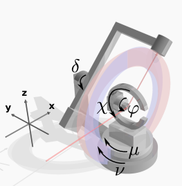
Figure 2: sketch of a goniometer with three sample axis, and two detector rotations. A red and a blue plane indicate the detector rotation planes of the inner detector rotation for two different positions of the outer detector arm rotation.

To elucidate the definition of a goniometer we use the goniometer shown in Fig. 2. The goniometer has a 3S+2D geometry, which means it offers three degrees of rotation for the sample and two independent degrees of freedom for the detector. The goniometer axes are specified by their axis direction and rotation sense. The coordinate system is chosen to have $x$ pointing downstream along the primary beam, $z$ is pointing upwards and $y$ pointing backwards to have a right-handed reference frame. In xrayutilities we describe each rotation axis with one character giving the axis direction (either x, y, or z) and the rotation sense (either + or -). This description needs to be supplied for the sample and detector circles for the case where all axis are at zero position starting with the outermost circle. The goniometer in Fig. 2 has three sample circles ($\mu$, $\chi$, $\varphi$) with the indicated rotation directions. The outermost angle $\mu$ turns clockwise around the $z$-coordinate axis and thus is described by ’z-’. The complete sample goniometer is described by the following set of rotations: (’z-’,’x-’,’y+’). For the detector circles turning around the $z$ and $y$-directions, the corresponding definition is (’z-’,’y-’). A full example of how to insert these definitions into xrayutilities is given in the appendix.

2.2 special rotation directions (Kappa goniometer)

In addition to rotations around axis of the coordinate system an often used goniometer geometry is the so called $\kappa$-geometry [Poot1972, Thorkildsen1999], in which one of the rotation axis has an angle of typically 45 to 60^∘ with one of the other axis. In xrayutilities we define such an axis by k+ or k-. The plane of the $\kappa$-rotation axis as well as its angle with respect to a reference direction are specified in a configuration file by the options kappa_plane and kappa_angle. The rotation matrix needed in matrix $\uuline{S}$ can be determined easily using an general equation given in the appendix.

3 Angular to momentum space conversion for 1D and 2D detectors

Equation 5 describes the conversion from angular coordinates of a general goniometer to reciprocal space for a point detector only. The generalization for a linear or area detector requires information about the pixel size and distance, and the direction into which a pixel row extends. Usually in the data files only one angular position is stored for every data point recorded with a multidimensional detector. This angular coordinate corresponds to the position of the so called center channel/pixel ($n_{0}$), which is the pixel hit by the primary beam when all the angles are set to zero. For all other detector pixels their position needs to be determined. This is easiest for the case of a curved one dimensional detector in which every detector channel or pixel covers the same detector angle segment. Every detector pixel (identified by the channel number $n$) corresponds to a detector angle $2\theta$ given by

$$2\theta(n)=2\theta_{0}+(n-n_{0})/N$$ (8)

where $N$ is the number of channels per unit of angle of the detector circle. When the detector angle is expressed in degree $N$ equals the number of channels per degree of rotation.

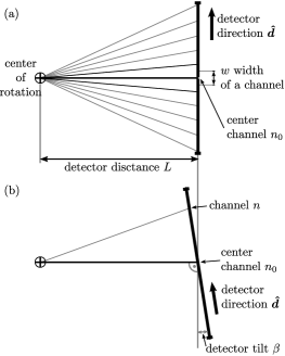
Figure 3: Sketch of a linear detector mounted at distance $L$ from the center of rotation of the goniometer. In (a) the detector direction specifying the direction along which higher channel numbers are found is given by $\boldsymbol{\hat{d}}$. Also indicated is the width of one channel $w$ and the center channel $n_{0}$, which is the channel where the primary beam is centered at zero detector angle. Panel (b) shows the possible detector tilt $\beta$ (misalignment), resulting if a detector is not mounted perfectly perpendicular to the X-ray beam.

Most modern detectors are, however, straight as shown in Fig. 3 and not curved and therefore Eq. 8 is not generally applicable. Only in the limit of a large sample detector distance the curved and straight detectors become indistinguishable. Nevertheless the channel per degree approximation is frequently used in practise. In xrayutilities one-dimensional detectors are treated as straight detectors and Eq. 5 is adjusted accordingly. For each detector pixel $n$, the corresponding direction of a scattered beam hitting this pixel is calculated, replacing Eq. 4 by

$$\boldsymbol{k}_{f}(n)=\left|\boldsymbol{k}_{i}\right|\uuline{D}\left(\boldsymbol{\hat{k}}_{i}+\boldsymbol{\hat{d}}(n-n_{0})w/L\right)/\|\boldsymbol{\hat{k}}_{i}+\boldsymbol{\hat{d}}(n-n_{0})w/L\|,$$ (9)

where $w$ and $L$ are the size of a detector pixel and distance from sample to detector as shown in Fig. 3. The direction in which the detector channel number increases is given by $\boldsymbol{\hat{d}}$. A ’hat’ on a vector indicates a unit vector. The fraction $w/L$ is in the case of large sample to detector distance equal to $1/N$, where $N$ is is the number of channels per radians, and Eq. 9 effectively simplifies to the form of Eq. 8. For a two dimensional detector with channel directions $\boldsymbol{\hat{d}}_{1}$ and $\boldsymbol{\hat{d}}_{2}$ we can write an equivalent equation for the exiting wave vector of channel ($n_{1}$,$n_{2}$) including the width of the detector pixels $w_{1,2}$ as

$$\boldsymbol{k}_{f}(n_{1},n_{2})=\left|\boldsymbol{k}_{i}\right|\uuline{D}\left(\boldsymbol{\hat{k}}_{i}+\boldsymbol{\hat{d}}_{1}(n_{1}-n_{1}^{(0)})w_{1}/L+\boldsymbol{\hat{d}}_{2}(n_{2}-n_{2}^{(0)})w_{2}/L\right)/\|\cdots\|,$$ (10)

Using the description of the detector in real space we do therefore avoid the ”channel per degree” approximation, which implicitly assumes a detector is curved and therefore does not work for small sample detector distances with large detectors. Inserting Eqs. 9 and 10 into Eq. 2 and 3 yields general equations for the reciprocal space conversion of linear and area detectors. The possible misalignments are included in those equations via the pixel directions $\boldsymbol{\hat{d}}$ for the 1D and $\boldsymbol{\hat{d}}_{1,2}$ for the 2D detectors.

3.1 Detector parameters of 1D detectors

For the conversion algorithms described above several detector parameters are needed. Among them the detector distance $L$ and width of one detector channel $w$. Since neither the detector distance nor the width of one channel can be easily measured very accurately, we use the fact that only their ratio is needed, which can be determined from an angular scan through the primary beam. Assume a linear detector is mounted along the direction in which the detector arm of the used instrument moves. Scanning the detector angle will move the primary beam over the detector, by modeling this movement we are able to determine the needed quantities. Therefore assume a linear detector mounted at a distance $L$ like the one shown in Fig. 3. Neglecting for the moment a possible detector tilt, i. e. when a detector is not mounted perfectly perpendicular to the X-ray beam, the detector channel at which the detector is hit for a detector arm angle $2\theta$ is given by

$$n(2\theta)=\frac{L}{w}\tan 2\theta+n_{0}.$$ (11)

If a detector tilt $\beta$ as shown in Fig. 3 is included above equation needs to be modified and one finds

$$n(2\theta,\beta)=\frac{L}{w}\frac{\sin 2\theta}{\cos\left(2\theta-\beta\right)}+n_{0}.$$ (12)

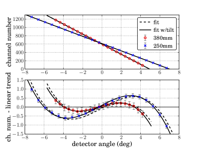
Figure 4: Determination of the ratio $w/L$ and center channel for a linear detector with pixel size of 50 $\mu$m from the variation of the beam position during a scan through the primary beam by fitting Eq. 12 to the recorded data. Shown are the channel numbers at which the beam is observed vs. the detector angle during the scan. The lower plot shows the experimental data as well as the fits when the linear trend is subtracted. A fit with (full line) and without (dashed line) considering a detector tilt is shown for two detector distances of 250 mm and 380 mm.

By fitting one of the two models one can find the necessary detector parameters needed for the reciprocal space conversion of a linear detector. For this purpose a scan through the primary beam should be performed with the linear detector and the detector spectra should be saved at every position. Since not only the slope is determined (which only needs two spectra), it is required to acquire several spectra, we suggest typically $\gtrsim 10$. For the determination of the parameters two functions are provided in xrayutilities. One of them automatically processes the spectra of a linear detector acquired during a scan through the primary beam and determines the position of the primary beam in every spectrum by fitting a Gaussian peak. From this fitting the position of the primary beam is found with sub-pixel precision. The second function needs the user to determine the channel number of the primary beam and supply it to the function, which should be used only in cases the first function is not applicable. Calling one of the two functions will produce a plot as the one shown in Fig. 4, which shows the channel number at which the beam was hitting the detector together with the variation expected from the model(s). A second subplot shows the comparison of model and measured data with the linear trend subtracted, for two different detector distances of 380 mm and 250 mm for a straight linear detector with a pixel size of 50 $\mu$m. The different distance shows up as different slope in the upper subplot. When the linear trend is subtracted the non-linearity due to the trigonometric functions in Eqs. 11 and 12 can be seen. The fit is also sensitive to a tilt of the detector from the direction perpendicular to the primary beam as can be seen from the comparison of the model without tilt (Eq. 11, dashed line) and model with tilt (Eq. 12, full line). For the measurements shown in Fig. 4 an artificial tilt of 0.3 deg was introduced, which was also determined by the fit. Note that a tilt of the detector is not only a result of a not perfectly mounted detector, but can also result from the fact that experimentalists choose to use a center channel, which does not correspond to the true center of the detector and do this by redefining the zero position of the detector arm rotation, which introduces a tilting of the detector by exactly the angle by which the detector arm angle changed! Using a translation of the detector perpendicular to the beam (mounted on top of the detector arm) would prevent such a tilt, is, however, very often not available.

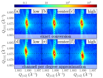
Figure 5: Six reciprocal space maps recorded around the Si (331) Bragg peak using the same sample movement, however, using different parts of a linear detector for detection. The white cross marks the nominal position of the Si (331) Bragg peak. Panels (a,d) were recorded when the detector was offset to lower angles, panels (c,f) with an offset to higher angles, whereas panels (b,e) were recorded with the signal centered on the detector. For panels (a) to (c) the exact reciprocal space conversion described in the text was used, whereas for panels (d) to (f) the ”channel per degree” approximation was applied leading to errors in the observed peak positions.

Basically this shows the necessity of non-linear models instead of the simpler linear fitting, which is a reasonable approximation only in the case of a large sample to detector distance. If a linear or area detector covers an angular range of $\gtrsim 8^{\circ}$ it gets absolutely necessary to use the above treatment since deviations would exceed one channel for typical channel sizes of around 50 $\mu$m. Using large linear detectors at moderate sample detector distances this limit is frequently reached especially in modern laboratory diffractometers. To further highlight the necessity of the non-linear models we show an example of a x-ray diffraction reciprocal space map measurement of the Si (331) Bragg peak of a Si(111) oriented single crystal in Fig. 5. The measurement was performed with the above mentioned linear detector at a distance of 250 mm at a laboratory diffractometer with CuK$\alpha$1 radiation produced by a Ge(220) channel cut monochromator. The same measurement was repeated three times, however, different parts of the detector were used for the detection of the diffracted signal. We compare the reciprocal space maps obtained using our exact conversion formalism in comparison with the ”channel per degree” approximation which assumes a curved detector like described by Eq. 8. Using this approximation (panels (d) to (f) in Fig. 5) we find that only the measurement using the central part of the detector gives the correct peak position in reciprocal space/lattice parameter. The measurements performed with the detector offset to higher or lower angles would result in a lattice parameter wrong by approximately 0.04%, which is far beyond the usual sensitivity of the experimental setup, which is said to be $<1\times 10^{-4}$ and can be increased further as for example outlined in [Fewster1999]. Using the accurate conversion no such shifts are observed and the three measurements (panels (a) to (c)) are indeed equivalent.

3.2 Detector parameters of 2D detectors

For 2D detectors similar determination of the $w_{1,2}/L$ ratio can be performed if the detector rotation and other misalignments (see below) are negligible, by decomposing the problem into two separate one dimensional problems. In case the detector is rotated around the primary beam the problem can no longer be decomposed. In particular one more problem specific to two dimensional detectors arises. Very often the true zero of the outer detector arm rotation is not known. For the inner detector rotation this does not imply any particular problem since it shows up only as additional tilt, which can be easily corrected. However, an offset in the outer detector rotation implies a rotation of the rotation axis of the inner detector rotation. In case the outer motor is not at the true zero the inner rotation will no longer rotate perpendicular to the primary beam as indicated by the two rotation planes shown in Fig. 2. In case the outer motor would be at its true zero the detector would rotate in the blue plane, due to an offset in the outer rotation the detector instead rotates in the red plane. This means the offset of the outer motor needs to be determined from alignment scans as well.

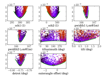
Figure 6: Determination of detector parameters. Shown is the optimization error vs. the eight considered parameters: the center channels of the detector and the width of the pixels in both directions, the detector tilt (azimuth and tilt angle), the detector rotation and the offset of the outer goniometer stage. The found optimum is marked by a black circle. All other points correspond to fits which did not reach the global minimum, those were produced from various different starting parameters of the fit. Green lines are guides to the eye to visualize the minimum found in all the parameters. The points of the fits are colored to enable the identification of correlations.

In general one needs to determine 8 parameters for a 2D detector: the center channels ($n_{1}^{(0)}$, $n_{2}^{(0)}$), the ratios $w_{1}/L$ and $w_{2}/L$, and directions of the vectors $\boldsymbol{\hat{d}}_{1,2}$ which are specified by the tilt, tilt direction and rotation of the detector around the primary beam and the outer angle offset described above. The untilted directions of the vectors $\boldsymbol{\hat{d}}_{1,2}$ can be determined by knowledge of the primary beam and detector rotation directions unambiguously and do therefore not need to be included in the fit. Similar as for the one dimensional detector those parameters can be determined from scans through the primary beam. It is necessary to use at least two scans, one with the inner and one with outer detector arm rotation with sufficient points around the primary beam and acquire a detector image at several positions. From the primary beam position observed in those images the detector directions and other necessary parameters can be determined by a fitting routine. As quality criterion of the fit the average $\|\boldsymbol{q}\|$-value of the pixel at which the primary beam is observed is used. This position is calculated using Eqs. 3 and 10. Since it is the primary beam we observe in all the images, this $\|\boldsymbol{q}\|$-value should be zero when the correct detector parameters are found. xrayutilities provides a function which takes the detector images and performs a fit of the 8 described parameters. Since several of those parameters, e. g. the offset of the outer motor with one of the center channels, are coupled with each other, the fit is performed in a way that it starts from several starting parameters to find the global minimum in the parameter space. An example of such a fit is shown in Fig. 6. The detector parameters have been determined from two perpendicular scans through the primary beam using a Maxipix-detector with effectively 516 times 516 pixels at beamline ID01/ESRF [esrfid01]. One scan was performed using the outer detector arm motor (moving horizontal) and the other one with the inner detector circle (moving vertical). In each scan we used 70 points, which means that in total 140 images were used. Note that using considerable less number of points does reduce the quality of the fit until no reliable statement can anymore be made about the misalignment parameters. It is therefore suggested to use a comparable number of points as in this example. Furthermore the images were manually selected to use just those with the full primary beam in active area of the detector. These images were fed into the algorithm described above and the detector rotation, tilt, tilt azimuth and outer angle offset along with the center channels and detector pixel size were determined. This determination is shown in Fig. 6, were the average $\|\boldsymbol{q}\|$-deviation of the detector pixels positions associated with the primary beam in the performed scans is shown. The value of this deviation is approximately the offset of the absolute value of the momentum transfer in reciprocal space. This deviation shows a clear minimum in all the 8 parameters. These 8 parameters are: 1/2. cch1,2 are the center channels of the detector in both directions. This is the pixel number where the primary beam is hitting the detector at the true zero position of the detector arm (including the outer angle offset). 3/4. pwidth1,2 are the pixel widths of the pixels in the two detector directions. The unit of these values in the plot is the size of the pixels in $\mu$m assuming a detector distance of 1 m. This corresponds to the parameter $w/L$ from above. If the pixel size is known the detector distance can be calculated or vice versa. 5. tiltazimuth is an angle giving the direction of the detector tilt. An value of 90 and 270 degrees corresponds to a tilt rotation around the first pixel direction and 0 and 180 around the second pixel direction, respectively.

6. tilt is the tilt angle of the detector plane around the direction given by the tiltazimuth, since the tilt-azimuth runs from 0 to 360 only positive tilts are used. 7. detrot is the detector rotation around the primary beam direction in degrees. 8. outerangle offset is the offset of the outer detector arm rotation in degrees.

For the determination of those parameters fits with various different starting parameters are performed. This is absolutely mandatory since several of the parameters are correlated, and therefore a single fit would not necessarily find the global optimum. One correlation, which can be easily imagined is the correlation of one of the center channels with the outer rotation offset. Since the detector orientation is not given to the script and automatically determined from the given scan data it is not apriori clear if this is center channel 1 or 2. In Fig. 6 this correlation can be seen in the plot showing center channel 2 (cch2) and the outer angle offset. The cloud of points from center channel 2 is rather broad since this value changes when the outer angle offset is changed. In fact the coloring of the cloud of points of center channel 2 reveals that it is only mirrored with respect to the one of the outer angle offset. A not so intuitive correlation is the one of the detector tilt with the outer angle offset. Imagine a not tilted detector, which is however offset in the outer angle. Such an offset will effectively tilt the detector by exactly the offset in the outer angle with a tilt azimuth of 90 or 270 deg. In case the detector is already slightly tilted in an arbitrary direction without outer angle offset, the tilt due to an outer angle offset will overlay with the initial tilt and influence the tilt azimuth and tilt in a non-trivial manner. The optimal set of parameters for the area detector of beamline ID01 was determined from the point with the lowest lowest error (global minimum in the parameter space) of $2.70\times 10^{-9}$.

To elucidate the benefit of considering those “misalignment” parameter, which are usually omitted, we also give the obtained errors when several of the quantities are fixed. When only the center channels and pixel widths are fitted we obtain an error of $1.68\times 10^{-6}$, which is orders of magnitude higher than our optimal error. In the present example the most important parameter is the detector rotation which brings the error down to $3.65\times 10^{-9}$. The second most important parameter is the outer angle offset, which brings down the error further to $2.81\times 10^{-9}$. If only the tilt (tilt azimuth and tilt angle) or the outer angle offset are fitted without the detector rotation, the error can only be reduced by less than 10% from the value without considering any misalignment. Only when all parameters are considered in the fit the error can be reduced to the optimum. This clearly shows that all those parameters should be considered to obtain the correct reciprocal space positions of the full area detector.

It should be noted that some of the parameters like the offset of the outer detector arm rotation and detector tilt can only be determined when the detector is spanning a certain angular range, the user is therefore urged to check the resulting plots in order to see if the parameters are reasonable. In cases where the detector distance is large the outer angle offset can only be determined with large error and it might be better to fix the corresponding parameter during fitting. Also the in cases when the detector tilt is small the tilt azimuth will not have a clear minimum and is therefore a indeterminable parameter. The script also outputs the code needed for initialization of the area detector, which considers the determined tilts and rotations as shown in the appendix B. These detector tilts of linear and area detectors are then included in the reciprocal space conversion. When the detector pixel position is calculated as described in Eq. 9 and 10 the detector direction $\boldsymbol{\hat{d}}$ or $\boldsymbol{\hat{d}}_{1,2}$ need to be rotated accordingly before the detector position is calculated.

In case no detector rotations are available, e. g. when using an area detector for powder diffraction we refer to the fit2d software [fit2d] for determining the necessary parameters.

4 Conclusions

In conclusion we present algorithms for reciprocal space conversion for X-ray diffraction experiments. We generalize the equations given by [Busing1967, You1999] for the use of linear and area detectors. Using our approach we can convert angles from arbitrary goniometers to reciprocal space coordinates. For the conversion of linear and area detectors several detector parameters, including all possible misalignments are needed. Recipes were presented how those parameters can be determined from alignment scans for both linear and area detectors. The software package including the presented algorithms is available at http://xrayutilities.sourceforge.net. The algorithms were shown to determine the detector parameters of a 1D and 2D detectors, which are otherwise not determinable.

Appendix A Implementation details

The software package is available from http://xrayutilities.sourceforge.net and is mainly coded in the popular scripting language Python™ with some performance critical parts written internally in the C programming language. The user needs to use only the Python package. Installation is possible on all major platforms (Windows, Mac, Linux/Unix). In addition to the reciprocal space conversion the package offers several functions to read data from spec-files, spectra-files and from laboratory diffractometers of Panalytical (xrdml) and Seifert (nja) as well as several CCD-data files (edf,tiff) and other function, which are described in the documentation found at the web-page.

The reciprocal space conversions performance critical part, which implements Eq. 5 and equivalents for linear and area detectors is coded in C. As can be seen from Eq. 5 it mainly consists of $3\times 3$ matrix operations. For the conversion of angular positions the matrices of the sample rotations need to be set up, for which the rotation matrices as the one shown in Eq. 7 are used. These matrices are multiplied in the order as given in Eq. 6. Furthermore, the conversion involves one matrix inversion, which is performed using the adjugate matrix formula. For matrix $\uuline{A}$ this means the inverse is given by

$$\uuline{A}^{-1}=\frac{\operatorname{adj}\uuline{A}}{\operatorname{det}\uuline{A}}\text{ .}$$ (13)

Depending on the number of sample ($n_{s}$) and detector circles ($n_{d}$) to be considered in the conversion for a point detector $n_{s}+n_{d}+2$ matrix multiplications, the matrix inversion, and one matrix-vector multiplication as well as one matrix-matrix subtraction need to be performed for every data point.

However, for linear and area detectors not for every detector pixel all the conversion needs to be done. For one spectrum or image all the sample and detector angles are considered to be constant and therefore the $n_{s}+n_{d}+1$ matrix multiplications as well as the matrix inversion need to be performed only once. Only two matrix-vector multiplications and some vector arithmetic to set up the pixel position need to be performed for every detector channel/pixel which enables a fast conversion also for large area detectors. Furthermore, the conversion for multiple data points is independent and can therefore be easily performed in parallel on modern multiprocessor computers.

Appendix B example script for the reciprocal space conversion

In the following an example script for the conversion of an image from an area detector recorded using the goniometer shown in Fig. 2 is given. This goniometer has the sample angles $\mu$, $\chi$ and $\phi$ and detector angles $\nu$ and $\delta$. The rotation axis of this goniometer are as given in the main text (sample circles: (’z-’,’x-’,’y+’) and detector circles: (’z-’,’y+’)) and the primary beam propagates along positive $x$-direction. The script is written in the Python™ script language.

import xrayutilities as xu

Nav = (1,1) # number of pixel to average over (reduce amount of data)
region_of_interest = (100,500,100,500) # region of interest on detector
en = 9000 # xray energy in eV

qconv = xu.QConversion((’z-’,’x-’,’y+’),(’z-’,’y-’),(1,0,0))
# 3S+2D goniometer: sample rotations: mu,chi,phi: (’z-’,’x-’,’y+’);
# detector rotations: nu,delta: (’z-’,’y-’)
# primary beam direction (1,0,0)

Si = xu.materials.Si
hxrd = xu.HXRD(Si.Q(1,0,0),Si.Q(0,1,0),en=en,qconv=qconv)
hxrd.Ang2Q.init_area(’z-’,’y+’,cch1=300.11,cch2=320.78,Nch1=516,Nch2=516,
    pwidth1=1.6639e-04,pwidth2=1.6630e-04,distance=1.,detrot=-0.749,
    tiltazimuth=3.0,tilt=0.448,Nav=Nav,roi=region_of_interest)
outerangle_offset = -0.643

# experimental goniometer angles
mu,chi,phi = (20,0,0)
nu,delta = (40,0)

# conversion to Q
qx,qy,qz = hxrd.Ang2Q.area(mu,chi,phi,nu,delta,delta=(0,0,0,outerangle_offset,0))

# conversion to (h,k,l)
h,k,l = hxrd.Ang2HKL(mu,chi,phi,nu,delta,delta=(0,0,0,outerangle_offset,0),
                     mat=Si,dettype=’area’)

All the detector parameters (like center channels, number of pixels, size of the pixels and the distance as well as possible tilts and rotations of the detector) need to be given to the $\tt init\_area$-function. This parameters are the result of a fit like the one shown in Fig. 6. The conversion is then performed by calling the area-method of an experiment class object, where also the outerangle offset needs do be considered. An experiment object holds information about the experiment like orientation of the crystal on top of innermost sample circle, the goniometer geometry and the X-ray energy. Here the object is initialized for an experiment performed using X-rays with an energy of 9000 eV and silicon crystal with the [100] direction along the primary beam at zero position and [010] along the $z$-axis. The second argument [010] gives the reference direction perpendicular to the primary beam in the plane spanned by the innermost detector direction. Dummy values for the reference directions can be used when the Ang2HKL function is not used!

After execution of this script the variables qx, qy and qz hold the reciprocal space position of the detector pixels specified by the region of interest variable. In the case above those variables will have a shape of 400$\times$400, holding the $q$-position of the pixels 100 to 500 in both detector directions. The variable Nav could be used to reduce the amount of data by block averaging. Using Nav = (2,2) effectively quadruples the area covered by one pixel and therefore reduces number of returned $q$-positions to 200$\times$200 per coordinate.

Furthermore the use of the algorithms to directly convert angles to reciprocal space indices $h$, $k$ and $l$ is shown. A function named Ang2HKL, which is called together with the orientation matrix to directly convert the experimental angles to the indices $h$, $k$, $l$ instead of the momentum transfer in units of Å^-1. Instead of specifying the orientation matrix one can also use the crystallographic orientation of the sample to determine the matrix $\uuline{U}$, which is the default if no $\uuline{U}$-matrix is explicitly given. Special algorithms also exist for determining the matrix $\uuline{B}$ from unit cell vectors. In the example the matrix $\uuline{B}$ is determined directly from the built in Material properties of silicon. In the present case (horizontal diffraction) the momentum transfer for the area detector has mainly a component along negative $y$-direction, whereas the $h$, $k$, $l$ components have there largest component along $l$.

Experimental angles do of course not need to be entered manually. They can be read from several different data formats as mentioned above. Details are given in the documentation found online.

Appendix C rotation matrix for arbitrary axis direction

Several rotations need to be performed around none primitive directions, e. g. in the case of $\kappa$-goniometers or also when calculating detector tilts. In such case the rotation axis as well as the angle of rotation are known and rotation matrices are generated using an formula given in [Lang1998]. The components or the rotation matrix $(\uuline{R})_{ij}=r_{ij}$ for rotation of angle $\alpha$ around the axis $\boldsymbol{e}$ are given by

$$r_{ij}=e_{i}e_{j}+(\delta_{ij}-e_{i}e_{j})\cos\alpha-\epsilon_{ijk}e_{k}\sin\alpha$$ (14)

with the Kronecker delta $\delta_{ij}$ and the Levi-Civita symbol $\epsilon_{ijk}$.

Acknowledgements

We acknowledge the help of our local contact for the measurements performed at the synchrotron beamline ID01 ESRF Grenoble (T. Schülli) and the financial support of the Austrian Science fund (IRON SFB25). DK acknowledges the support by Austrian Academy of Sciences (DOC-fellowship). Special thanks also to the early users for their feedback (T. Etzelstorfer, M. Keplinger, R. Grifone, S. Cecchi).

References

- [1] \harvarditemBond1960Bond1960 Bond, W. L. \harvardyearleft1960\harvardyearright. Acta Cryst. \volbf13(10), 814.
- [2] \harvarditemBunk \harvardand Nielsen2004Bunk2004 Bunk, O. \harvardand Nielsen, M. M. \harvardyearleft2004\harvardyearright. J. Appl.Cryst. \volbf37(2), 216.
- [3] \harvarditemBusing \harvardand Levy1967Busing1967 Busing, W. R. \harvardand Levy, H. A. \harvardyearleft1967\harvardyearright. Acta Cryst. \volbf22(4), 457.
- [4] \harvarditem[Diaz et al.]Diaz, Mocuta, Stangl, Mandl, David, Vila-Comamala, Chamard, Metzger \harvardand Bauer2009Diaz2009 Diaz, A., Mocuta, C., Stangl, J., Mandl, B., David, C., Vila-Comamala, J., Chamard, V., Metzger, T. H. \harvardand Bauer, G. \harvardyearleft2009\harvardyearright. Phys. Rev. B, \volbf79, 125324.
- [5] \harvarditemFewster1999Fewster1999 Fewster, P. F. \harvardyearleft1999\harvardyearright. J. Mater. Sci.: Mater. Electron. \volbf10, 175 – 183.
- [6] \harvarditemFienup1982Fienup1982 Fienup, J. R. \harvardyearleft1982\harvardyearright. Appl. Opt. \volbf21, 2758–2769.
- [7] \harvarditemHammersley2013fit2d Hammersley, A., \harvardyearleft2013\harvardyearright. fit2d. http://www.esrf.eu/computing/scientific/FIT2D/index.html.
- [8] \harvarditemKriegner \harvardand Wintersberger2013xrutils_web Kriegner, D. \harvardand Wintersberger, E., \harvardyearleft2013\harvardyearright. http://xrayutilities.sourceforge.net.
- [9] \harvarditemLang \harvardand Pucker1998Lang1998 Lang, C. B. \harvardand Pucker, N. \harvardyearleft1998\harvardyearright. Mathematische Methoden in der Physik. Spektrum Akad. Verl. Heidelberg Berlin.
- [10] \harvarditemLeslie2006Leslie2006 Leslie, A. G. W. \harvardyearleft2006\harvardyearright. Acta Cryst. D, \volbf62, 48–57.
- [11] \harvarditemLohmeier \harvardand Vlieg1993Lohmeier1993 Lohmeier, M. \harvardand Vlieg, E. \harvardyearleft1993\harvardyearright. J Appl. Cryst. \volbf26(5), 706.
- [12] \harvarditem[Lutterotti et al.]Lutterotti, Matthies \harvardand Wenk1999Lutterotti1999 Lutterotti, L., Matthies, S. \harvardand Wenk, H.-R. \harvardyearleft1999\harvardyearright. IUCr: Newsletter of the CPD, \volbf21, 14–15.
- [13] \harvarditem[Miao et al.]Miao, Sayre \harvardand Chapman1998Miao1998 Miao, J., Sayre, D. \harvardand Chapman, H. N. \harvardyearleft1998\harvardyearright. J. Opt. Soc. Am. A, \volbf15, 1662–1669.
- [14] \harvarditemMicrodiffraction imaging beamline ID01 - ESRF Grenoble2013esrfid01 Microdiffraction imaging beamline ID01 - ESRF Grenoble, \harvardyearleft2013\harvardyearright. http://www.esrf.eu/UsersAndScience/Experiments/StructMaterials/ID01.
- [15] \harvarditem[Minkevich et al.]Minkevich, Fohtung, Slobodskyy, Riotte, Grigoriev, Schmidbauer, Irvine, Novák, Holý \harvardand Baumbach2011Minkevich2011 Minkevich, A. A., Fohtung, E., Slobodskyy, T., Riotte, M., Grigoriev, D., Schmidbauer, M., Irvine, A. C., Novák, V., Holý, V. \harvardand Baumbach, T. \harvardyearleft2011\harvardyearright. Phys. Rev. B, \volbf84, 054113.
- [16] \harvarditemPasserelle2013passerelle Passerelle, \harvardyearleft2013\harvardyearright. component-based solution assembly suite. https://code.google.com/a/eclipselabs.org/p/passerelle/.
- [17] \harvarditem[Pietsch et al.]Pietsch, Holy \harvardand Baumbach2004Pietsch2004 Pietsch, U., Holy, V. \harvardand Baumbach, T. \harvardyearleft2004\harvardyearright. High-Resolution X-Ray Scattering: From Thin Films to Lateral Nanostructures. Advanced Texts in Physics. New York: Springer.
- [18] \harvarditemPoot1972Poot1972 Poot, S. \harvardyearleft1972\harvardyearright. US Patent No. , p. 3 636 347.
- [19] \harvarditemRodriguez-Carvajal2001Rodriguez2001 Rodriguez-Carvajal, J. \harvardyearleft2001\harvardyearright. Commission on Powder Diffraction (IUCr) Newsletter, \volbf26, 12–19.
- [20] \harvarditemspec2013certif spec \harvardyearleft2013\harvardyearright. Certified Scientific Software PO Box 390640, Cambridge, MA 02139, USA.
- [21] \harvarditem[Stangl et al.]Stangl, Holý \harvardand Bauer2004Stangl2004 Stangl, J., Holý, V. \harvardand Bauer, G. \harvardyearleft2004\harvardyearright. Rev. Mod. Phys. \volbf76, 725–783.
- [22] \harvarditem[Thorkildsen et al.]Thorkildsen, Mathiesen \harvardand Larsen1999Thorkildsen1999 Thorkildsen, G., Mathiesen, R. H. \harvardand Larsen, H. B. \harvardyearleft1999\harvardyearright. J. Appl. Cryst. \volbf32(5), 943.
- [23] \harvarditemWarren1969Warren1969 Warren, B. E. \harvardyearleft1969\harvardyearright. X-Ray Diffraction. Dover Books on Physics Series. Dover Publ.
- [24] \harvarditem[Wintersberger et al.]Wintersberger, Kriegner, Hrauda, Stangl \harvardand Bauer2010Wintersberger2010 Wintersberger, E., Kriegner, D., Hrauda, N., Stangl, J. \harvardand Bauer, G. \harvardyearleft2010\harvardyearright. J. Appl. Cryst. \volbf43(6), 1287.
- [25] \harvarditemYou1999You1999 You, H. \harvardyearleft1999\harvardyearright. J. Appl. Cryst. \volbf32(4), 614.
- [26]