Solving Heat Conduction Problems by the Direct Meshless Local Petrov-Galerkin (DMLPG) method

Abstract

As an improvement of the Meshless Local Petrov–Galerkin (MLPG), the Direct Meshless Local Petrov–Galerkin (DMLPG) method is applied here to the numerical solution of transient heat conduction problem. The new technique is based on direct recoveries of test functionals (local weak forms) from values at nodes without any detour via classical moving least squares (MLS) shape functions. This leads to an absolutely cheaper scheme where the numerical integrations will be done over low–degree polynomials rather than complicated MLS shape functions. This eliminates the main disadvantage of MLS based methods in comparison with finite element methods (FEM), namely the costs of numerical integration.

1 Introduction

Meshless methods have received much attention in recent decades as new tools to overcome the difficulties of mesh generation and mesh refinement in classical mesh-based methods such as the finite element method (FEM) and the finite volume method (FVM).

The classification of numerical methods for solving PDEs should always start from the classification of PDE problems themselves into strong, weak, or local weak forms. The first is the standard pointwise formulation of differential equations and boundary conditions, the second is the usual weak form dominating all FEM techniques, while the third form splits the integrals of the usual global weak form into local integrals over many small subdomains, performing the integration by parts on each local integral. Local weak forms are the basis of all variations of the Meshless Local Petrov–Galerkin technique (MLPG) of S.N. Atluri and collaborators atluri:2005-1 . This classification is dependent on the PDE problem itself, and independent of numerical methods and the trial spaces used. Note that these three formulations of the “same” PDE and boundary conditions lead to three essentially different mathematical problems that cannot be identified and need a different mathematical analysis with respect to existence, uniqueness, and stability of solutions.

Meshless trial spaces mainly come via Moving Least Squares or kernels like Radial Basis Functions. They can consist of global or local functions, but they should always parametrize their trial functions “entirely in terms of nodes” belytschko-et-al:1996-1 ; wendland:2005-1 and require no triangulation or meshing.

A third classification of PDE methods addresses where the discretization lives. Domain type techniques work in the full global domain, while boundary type methods work with exact solutions of the PDE and just have to care for boundary conditions. This is independent of the other two classifications.

Consequently, the literature should confine the term “meshless” to be a feature of trial spaces, not of PDE problems and their various formulations. But many authors reserve the term truly meshless for meshless methods that either do not require any discretization with a background mesh for calculating integrals or do not require integration at all. These techniques have a great advantage in computational efficiency, because numerical integration is the most time–consuming part in all numerical methods based on local or global weak forms. This paper focuses on a truly meshless method in this sense.

Most of the methods for solving PDEs in global weak form, such as the Element-Free Galerkin (EFG) method belytschko-et-al:1994-1 , are not truly meshless because a triangulation is still required for numerical integration. The Meshless Local Petrov-Galerkin (MLPG) method solves PDEs in local weak form and uses no global background mesh to evaluate integrals because everything breaks down to some regular, well-shaped and independent sub-domains. Thus the MLPG is known as a truly meshless method.

We now focus on meshless methods using Moving Least Squares as trial functions. If they solve PDEs in global or local weak form, they still suffer from the cost of numerical integration. In these methods, numerical integrations are traditionally done over MLS shape functions and their derivatives. Such shape functions are complicated and have no closed form. To get accurate results, numerical quadratures with many integration points are required. Thus the MLS subroutines must be called very often, leading to high computational costs. In contrast to this, the stiffness matrix in finite element methods (FEMs) is constructed by integrating over polynomial basis functions which are much cheaper to evaluate. This relaxes the cost of numerical integrations. For an account of the importance of numerical integration within meshless methods, we refer the reader to babuska-et-al:2009-1 .

To overcome this shortage within the MLPG based on MLS, Mirzaei and Schaback mirzaei-schaback:2011-1 proposed a new technique, Direct Meshless Local Petrov-Galerkin (DMLPG) method, which avoids integration over MLS shape functions in MLPG and replaces it by the much cheaper integration over polynomials. It ignores shape functions completely. Altogether, the method is simpler, faster and often more accurate than the original MLPG method. DMLPG uses a generalized MLS (GMLS) method of mirzaei-et-al:2012-1 which directly approximates boundary conditions and local weak forms as some functionals, shifting the numerical integration into the MLS itself, rather than into an outside loop over calls to MLS routines. Thus the concept of GMLS must be outlined first in Section 2 before we can go over to the DMLPG in Section 4 and numerical results for heat conduction problems in Section 6.

The analysis of heat conduction problems is important in engineering and applied mathematics. Analytical solutions of heat equations are restricted to some special cases, simple geometries and specific boundary conditions. Hence, numerical methods are unavoidable. Finite element methods, finite volume methods, and finite difference methods have been well applied to transient heat analysis over the past few decades minkowycz-et-al:1988-1 . MLPG methods were also developed for heat transfer problems in many cases. For instance, J. Sladek et.al. sladek-et-al:2003-1 proposed MLPG4 for transient heat conduction analysis in functionally graded materials (FGMs) using Laplace transform techniques. V. Sladek et.al. sladek-et-al:2005-2 developed a local boundary integral method for transient heat conduction in anisotropic and functionally graded media. Both authors and their collaborators employed MLPG5 to analyze the heat conduction in FGMs sladek-et-al:2004-1 ; sladek-et-al:2007-1 .

The aim of this paper is the development of DMLPG methods for heat conduction problems. This is the first time where DMLPG is applied to a time–dependent problem. Moreover, compared to mirzaei-schaback:2011-1 , we will discuss all DMLPG methods, go into more details and provide explicit formulae for the numerical implementation. DMLPG1/2/4/5 will be proposed, and the reason of ignoring DMLPG3/6 will be discussed. The new methods will be compared with the original MLPG methods in a test problem, and then a problem in FGMs will be treated by DMLPG1.

In all application cases, the DMLPG method turned out to be superior to the standard MLPG technique, and it provides excellent accuracy at low cost.

2 Meshless methods and GMLS approximation

Whatever the given PDE problem is and how it is discretized, we have to find a function $u$ such that $M$ linear equations

$$\lambda_{k}(u)=\beta_{k},\;1\leqslant k\leqslant M,$$ (1)

defined by $M$ linear functionals $\lambda_{1},\ldots,\lambda_{M}$ and $M$ prescribed real values $\beta_{1},\ldots,\beta_{M}$ are to be satisfied. Note that weak formulations will involve functionals that integrate $u$ or a derivative against some test function. The functionals can discretize either the differential equation or some boundary condition.

Now meshless methods construct solutions from a trial space whose functions are parametrized “entirely in terms of nodes” belytschko-et-al:1996-1 . We let these nodes form a set $X:=\{x_{1},\ldots,x_{N}\}$. Theoretically, meshless trial functions can then be written as linear combinations of shape functions $u_{1},\ldots,u_{N}$ with or without the Lagrange conditions $u_{j}(x_{k})=\delta_{jk},\;1\leqslant j,k\leq N$ as

$$u(x)=\sum_{j=1}^{N}u_{j}(x)u(x_{j})$$

in terms of values at nodes, and this leads to solving the system (1) in the form

$$\lambda_{k}(u)=\sum_{j=1}^{N}\lambda_{k}(u_{j})u(x_{j})=\beta_{k},\;1\leqslant k\leqslant M$$

approximately for the nodal values. Setting up the coefficient matrix requires the evaluation of all functionals on all shape functions, and this is a tedious procedure if the shape functions are not cheap to evaluate, and it is even more tedious if the functionals consist of integrations of derivatives against test functions.

But it is by no means mandatory to use shape functions at this stage at all. If each functional $\lambda_{k}$ can be well approximated by a formula

$$\lambda_{k}(u)\approx\sum_{j=1}^{N}\alpha_{jk}u(x_{j})$$ (2)

in terms of nodal values for smooth functions $u$, the system to be solved is

$$\sum_{j=1}^{N}\alpha_{jk}u(x_{j})=\beta_{k},\;1\leqslant k\leqslant M$$ (3)

without any use of shape functions. There is no trial space, but everything is still written in terms of values at nodes. Once the approximate values $u(x_{j})$ at nodes are obtained, any multivariate interpolation or approximation method can be used to generate approximate values at other locations. This is a postprocessing step, independent of PDE solving.

This calls for efficient ways to handle the approximations (2) to functionals in terms of nodal values. We employ a generalized version of Moving Least Squares (MLS), adapted from mirzaei-et-al:2012-1 , and without using shape functions.

The techniques of mirzaei-et-al:2012-1 and mirzaei-schaback:2011-1 allow to calculate coefficients $\alpha_{jk}$ for (2) very effectively as follows. We fix $k$ and consider just $\lambda:=\lambda_{k}$. Furthermore, the set $X$ will be formally replaced by a much smaller subset that consists only of the nodes that are locally necessary to calculate a good approximation of $\lambda_{k}$, but we shall keep $X$ and $N$ in the notation. This reduction of the node set for the approximation of $\lambda_{k}$ will ensure sparsity of the final coefficient matrix in (3).

Now we have to calculate a coefficient vector $a(\lambda_{k})=(\alpha_{1k},\ldots,\alpha_{Nk})^{T}\in\mathbb{R}^{N}$ for (2) in case of $\lambda=\lambda_{k}$. We choose a space $\mathcal{P}$ of polynomials which is large enough to let zero be the only polynomial $p$ in $\mathcal{P}$ that vanishes on $X$. Consequently, the dimension $Q$ of $\mathcal{P}$ satisfies $Q\leqslant N$, and the $Q\times N$ matrix $P$ of values $p_{i}(x_{j})$ of a basis $p_{1},\ldots,p_{Q}$ of $\mathcal{P}$ has rank $Q$. Then for any vector $w=(w_{1},\ldots,w_{N})^{T}$ of positive weights, the generalized MLS solution $a(\lambda)$ to (2) can be written as

$$a(\lambda_{k})=WP^{T}(P\,W\,P^{T})^{-1}\lambda_{k}(\mathcal{P})$$ (4)

where $W$ is the diagonal matrix with diagonal $w$ and $\lambda_{k}(\mathcal{P})\in\mathbb{R}^{Q}$ is the vector with values $\lambda_{k}(p_{1}),\ldots,\lambda_{k}(p_{Q})$.

Thus it suffices to evaluate $\lambda_{k}$ on low–order polynomials, and since the coefficient matrix in (4) is independent of $k$, one can use the same matrix for different $\lambda_{k}$ as long as $X$ does not change locally. This will significantly speed up numerical calculations, if the functional $\lambda_{k}$ is complicated, e.g. a numerical integration against a test function. Note that the MLS is just behind the scene, no shape functions occur. But the weights will be defined locally in the same way as in the usual MLS, e.g. we choose a continuous function $\phi:[0,\infty)\rightarrow[0,\infty)$ with

• $\phi(r)>0,~{}0\leqslant r<1,$

• $\phi(r)=0,~{}r\geqslant 1,$

and define

$$w_{j}(x)=\phi\left(\frac{\|x-x_{j}\|_{2}}{\delta}\right)$$

for $\delta>0$ as a weight function, if we work locally near a point $x$.

3 MLPG Formulation of Heat Conduction

In the Cartesian coordinate system, the transient temperature field in a heterogeneous isotropic medium is governed by the diffusion equation

$$\rho(x)c(x)\frac{\partial u}{\partial t}(x,t)=\nabla\cdot(\kappa\nabla u)+f(x,t),$$ (5)

where $x\in\Omega$ and $0\leqslant t\leqslant t_{F}$ denote the space and time variables, respectively, and $t_{F}$ is the final time. The initial and boundary conditions are

$$u(x,0) =u_{0}(x),\quad x\in\Omega,$$ (6)

$$u(x,t) =u_{D}(x,t),\quad x\in\Gamma_{D},\quad 0\leqslant t\leqslant t_{F},$$ (7)

$$\kappa(x)\frac{\partial u}{\partial n}(x,t) =u_{N}(x,t),\quad x\in\Gamma_{N},\quad 0\leqslant t\leqslant t_{F}.$$ (8)

In (5)-(8), $u(x,t)$ is the temperature field, $\kappa(x)$ is the thermal conductivity dependent on the spatial variable $x$, $\rho(x)$ is the mass density and $c(x)$ is the specific heat, and $f(x,t)$ stands for the internal heat source generated per unit volume. Moreover, $n$ is the unit outward normal to the boundary $\Gamma$, $u_{D}$ and $u_{N}$ are specified values on the Dirichlet boundary $\Gamma_{D}$ and Neumann boundary $\Gamma_{N}$ where $\Gamma=\Gamma_{D}\cup\Gamma_{N}$.

Meshless methods write everything entirely in terms of scattered nodes forming a set $X=\{x_{1},x_{2},\ldots,x_{N}\}$ located in the spatial domain $\Omega$ and its boundary $\Gamma$. In the standard MLPG, around each $x_{k}$ a small subdomain $\Omega_{s}^{k}\subset\overline{\Omega}=\Omega\cup\Gamma$ is chosen such that integrations over $\Omega_{s}^{k}$ are comparatively cheap. For instance, $\Omega_{s}^{k}$ is conveniently taken to be the intersection of $\overline{\Omega}$ with a ball $B(x_{k},r_{0})$ of radius $r_{0}$ or a cube (or a square in 2D) $S(x_{k},r_{0})$ centered at $x_{k}$ with side-length $r_{0}$. On these subdomains, the PDE including boundary conditions is stated in a localized weak form

$$\frac{\partial}{\partial t}\int_{\Omega_{s}^{k}}\rho cuv\,d\Omega=\int_{\Omega_{s}^{k}}\nabla\cdot(\kappa\nabla u)v\,d\Omega+\int_{\Omega_{s}^{k}}fv\,d\Omega,$$ (9)

for an appropriate test function $v$. Applying integration by parts, this weak equation can be partially symmetrized to become the first local weak form

$$\frac{\partial}{\partial t}\int_{\Omega_{s}^{k}}\rho cuv\,d\Omega=\int_{\partial\Omega_{s}^{k}}\kappa\frac{\partial u}{\partial n}\,v\,d\Gamma-\int_{\Omega_{s}^{k}}\kappa\nabla u\cdot\nabla v\,d\Omega+\int_{\Omega_{s}^{k}}fv\,d\Omega.$$ (10)

The second local weak form, after rearrangement of (5) and integration by parts twice, can be obtained as

$$\begin{split}\frac{\partial}{\partial t}\int_{\Omega_{s}^{k}}\frac{1}{\kappa}\rho cuv\,d\Omega&=\int_{\Omega_{s}^{k}}u\Delta v\,d\Omega-\int_{\partial\Omega_{s}^{k}}u\frac{\partial v}{\partial n}\,d\Gamma+\int_{\partial\Omega_{s}^{k}}v\frac{\partial u}{\partial n}\,d\Gamma\\ &+\int_{\Omega_{s}^{k}}\frac{1}{\kappa}\nabla\kappa\cdot\nabla u\,v\,d\Omega+\int_{\Omega_{s}^{k}}\frac{1}{\kappa}fv\,d\Omega.\end{split}$$ (11)

If the boundary of the local domain $\Omega_{s}^{k}$ hits the boundary of $\Omega$, the MLPG inserts boundary data at the appropriate places in order to care for boundary conditions. Since these local weak equations are all affine–linear in $u$ even after insertion of boundary data, the equations of MLPG are all of the form (1) after some rearrangement, employing certain linear functionals $\lambda_{k}$. In all cases, the MLPG evaluates these functionals on shape functions, while our DMLPG method will use the GMLS approximation of Section 2 without any shape function.

However, different choices of test functions $v$ lead to the six different well–known types of MLPG. The variants MLPG1/5/6 are based on the weak formulation (10). If $v$ is chosen such that the first integral in the right hand side of (10) vanishes, we have MLPG1. In this case $v$ should vanish on $\partial\Omega_{s}^{k}$. If the Heaviside step function $v$ on local domains is used as test function, the second integral disappears and we have a pure local boundary integral form in the right hand side. This is MLPG5. In MLPG6, the trial and test functions come from the same space. MLPG2/3 are based on the local unsymmetric weak formulation (9). MLPG2 employs Dirac’s delta function as the test function in each $\Omega_{s}^{k}$, which leads to a pure collocation method. MLPG3 employs the error function as the test function in each $\Omega_{s}^{k}$. In this method, the test functions can be the same as for the discrete least squares method. The test functions and the trial functions come from the same space in MLPG3. Finally, MLPG4 (or LBIE) is based on the weak form (11), and a modified fundamental solution of the corresponding elliptic spatial equation is employed as a test function in each subdomain.

We describe these types in more detail later, along with the way we modify them when going from MLPG to DMLPG.

4 DMLPG Formulations

Independent of which variation of MLPG we go for, the DMLPG has its special ways to handle boundary conditions, and we describe these first.

Neither Lagrange multipliers nor penalty parameters are introduced into the local weak forms, because the Dirichlet boundary conditions are imposed directly. For nodes $x_{k}\in\Gamma_{D}$, the values $u(x_{k},t)=u_{D}(x_{k},t)$ are known from the Dirichlet boundary conditions. To connect them properly to nodal values $u(x_{j},t)$ in neighboring points $x_{j}$ inside the domain or on the Neumann boundary, we turn the GMLS philosophy upside down and ask for coefficients $a_{j}(x_{k})$ that allow to reconstruct nodal values at $x_{k}$ from nodal values at the $x_{j}$. This amounts to setting $\lambda_{k}=\delta_{x_{k}}$ in Section 2 , and we get localized equations for Dirichlet boundary points $x_{k}$ as

$$\sum_{j=1}^{N}a_{j}(x_{k})u(x_{j},t)=u_{D}(x_{k},t),\quad x_{k}\in\Gamma_{D},\quad t\in[0,t_{F}].$$ (12)

Note that the coefficients are time–independent. In matrix form, (12) can be written as

$$B{\makebox{\boldmath$u$}}(t)={\makebox{\boldmath$u$}}_{D}(t),$$ (13)

where ${\makebox{\boldmath$u$}}(t)\in\mathbb{R}^{N}$ is the time–dependent vector of nodal values at $x_{1},x_{2},...,x_{N}$. These equations are added into the full matrix setup at the appropriate places, and they are in truly meshless form, since they involve only values at nodes and are without numerical integration. Note that (10) has no integrals over the Dirichlet boundary, and thus we can impose Dirichlet conditions always in the above strong form. For (11) there are two possibilities. We can impose the Dirichlet boundary conditions either in the local weak form or in the collocation form (12). Of course the latter is the cheaper one.

We now turn to Neumann boundary conditions. They can be imposed in the same way as Dirichlet boundary conditions by assuming $\lambda_{k}(u)=\frac{\partial u}{\partial n}(x_{k})$ in the GMLS approximation

$$\sum_{j=1}^{N}a_{j}(x_{k})u(x_{j},t)=\frac{\partial u}{\partial n}(x_{k},t),\quad x_{k}\in\Gamma_{N},\quad t\in[0,t_{F}].$$ (14)

Note that the coefficients again are time–independent, and we get a linear system like (13), but with a vector ${\makebox{\boldmath$u$}}_{N}(t)$ of nodal values of normal derivatives in the right–hand side. This is collocation as in subsection 4.2. But it is often more accurate to impose Neumann conditions directly into the local weak forms (10) and (11). We will describe this in more detail in the following subsections. We now turn the different variations of the MLPG method into variations of the DLMPG.

4.1 DMLPG1/5

These methods are based on the local weak form (10). This form recasts to

$$\begin{split}\frac{\partial}{\partial t}\int_{\Omega_{s}^{k}}\rho cuv\,d\Omega&+\int_{\Omega_{s}^{k}}\kappa\nabla u\cdot\nabla v\,d\Omega-\int_{\partial\Omega_{s}^{k}\setminus\Gamma_{N}}\kappa\frac{\partial u}{\partial n}v\,d\Gamma\\ &=\int_{\Gamma_{N}\cap\partial\Omega_{s}^{k}}u_{N}v\,d\Gamma+\int_{\Omega_{s}^{k}}fv\,d\Omega\end{split}$$ (15)

after inserting the Neumann boundary data from (8), when the domain $\Omega_{s}^{k}$ of (10) hits the Neumann boundary $\Gamma_{N}$. All integrals in the top part of (15) can be efficiently approximated by GMLS approximation of Section 2 as purely spatial formulas

$$\begin{array}[]{rclcl}\lambda_{1,k}(u)&:=&\displaystyle{\int_{\Omega_{s}^{k}}\rho cuv\,d\Omega}&\approx&\displaystyle{\widehat{\lambda_{1,k}(u)}=\sum_{j=1}^{N}a_{1,j}(x_{k})u(x_{j}),}\\ \lambda_{2,k}(u)&:=&\displaystyle{-\int_{\Omega_{s}^{k}}\kappa\nabla u\cdot\nabla v\,d\Omega}&\approx&\displaystyle{\widehat{\lambda_{2,k}(u)}=\sum_{j=1}^{N}a_{2,j}(x_{k})u(x_{j}),}\\ \lambda_{3,k}(u)&:=&\displaystyle{-\int_{\partial\Omega_{s}^{k}\setminus\Gamma_{N}}\kappa\frac{\partial u}{\partial n}v\,d\Gamma}&\approx&\displaystyle{\widehat{\lambda_{3,k}(u)}=\sum_{j=1}^{N}a_{3,j}(x_{k})u(x_{j})}.\end{array}$$ (16)

While the two others can always be summed up, the first formula, if applied to time–varying functions, has to be modified into

$${\frac{\partial}{\partial t}\int_{\Omega_{s}^{k}}\rho cuv\,d\Omega}\approx\displaystyle{\sum_{j=1}^{N}a_{1,j}(x_{k})\frac{\partial}{\partial t}u(x_{j},t)}$$

and expresses the main PDE term not in terms of values at nodes, but rather in terms of time derivatives of values at nodes.

Again, everything is expressed in terms of values at nodes, and the coefficients are time–independent. Furthermore, Section 2 shows that the $u$ part of the integration runs over low–order polynomials, not over any shape functions.

The third functional can be omitted if the test function $v$ vanishes on $\partial\Omega_{s}^{k}\setminus\Gamma_{N}$. This is DMLPG1. An example of such a test function is

$$v=v(x;x_{k})=\phi\left(\frac{\|x-x_{k}\|_{2}}{r_{0}}\right),$$

where $\phi$ is the weight function in the MLS approximation with the radius $\delta$ of the support of the weight function being replaced by the radius $r_{0}$ of the local domain $\Omega_{s}^{k}$.

In DMLPG5, the local test function is the constant $v=1$. Thus the functionals $\lambda_{2,k}$ of (16) are not needed, and the integrals for $\lambda_{1,k}$ take a simple form, if $c$ and $\rho$ are simple. DMLPG5 is slightly cheaper than DMLPG1, because the domain integrals of $\lambda_{2,k}$ are replaced by the boundary integrals of $\lambda_{3,k}$.

Depending on which parts of the functionals are present or not, we finally get a time–dependent system of the form

$$A^{(1)}\frac{\partial}{\partial t}{\makebox{\boldmath$u$}}(t)+A^{(\ell)}{\makebox{\boldmath$u$}}(t)={\makebox{\boldmath$b$}}(t),\quad\ell=2\,\,\mbox{or}\,\,3$$ (17)

where ${\makebox{\boldmath$u$}}(t)$ is the time–dependent vector

$${\makebox{\boldmath$u$}}(t)=(u(x_{1},t),\ldots,u(x_{N},t))^{T}\in\mathbb{R}^{N}$$

of nodal values, ${\makebox{\boldmath$b$}}(t)\in\mathbb{R}^{M}$ collects the time–dependent right–hand sides with components

$$b_{k}=\int_{\Omega_{s}^{k}}f(x,t)v(x;x_{k})\,d\Omega+\int_{\Gamma_{N}\cap\partial\Omega_{s}^{k}}u_{N}(x,t)v(x;x_{k})\,d\Gamma,$$

and $A_{kj}^{(\ell)}=a_{\ell,j}(x_{k})$, $\ell=1,2,3$. The $k$-th row of $A^{(\ell)}$ is

$${\makebox{\boldmath$a$}}_{k}^{(\mathrm{\ell})} =WP(PWP^{T})^{-1}\lambda_{\ell,k}(\mathcal{P}),\quad\ell=1,2,3,$$

where

$$\lambda_{1,k}(\mathcal{P})= \left[\int_{\Omega_{s}^{k}}\rho cp_{1}v\,d\Omega,\int_{\Omega_{s}^{k}}\rho cp_{2}v\,d\Omega,\ldots,\int_{\Omega_{s}^{k}}\rho cp_{Q}v\,d\Omega\right]^{T},$$

$$\lambda_{2,k}(\mathcal{P})= -\left[\int_{\Omega_{s}^{k}}\kappa\nabla p_{1}\cdot\nabla v\,d\Omega,\int_{\Omega_{s}^{k}}\kappa\nabla p_{2}\cdot\nabla v\,d\Omega,\ldots,\int_{\Omega_{s}^{k}}\kappa\nabla p_{Q}\cdot\nabla v\,d\Omega\right]^{T},$$

$$\lambda_{3,k}(\mathcal{P})= \left[\int_{\partial\Omega_{s}^{k}\setminus\Gamma_{N}}\kappa\frac{\partial p_{1}}{\partial n}v\,d\Gamma,\int_{\partial\Omega_{s}^{k}\setminus\Gamma_{N}}\kappa\frac{\partial p_{2}}{\partial n}v\,d\Gamma,\ldots,\int_{\partial\Omega_{s}^{k}\setminus\Gamma_{N}}\kappa\frac{\partial p_{Q}}{\partial n}v\,d\Gamma\right]^{T}.$$

As we can immediately see, numerical integrations are done over low-degree polynomials $p_{1},p_{2},...,p_{Q}$ only, and no shape function is needed at all. This reduces the cost of numerical integration in MLPG methods significantly.

4.2 DMLPG2

In this method, the test function $v$ on the local domain $\Omega_{s}^{k}$ in (9) is replaced by the test functional $\delta_{x_{k}}$, i.e. we have strong collocation of the PDE and all boundary conditions. Depending on where $x_{k}$ lies, one can have the functionals

$$\begin{array}[]{rcl}\mu_{1,k}(u)&:=&u(x_{k}),\\ \mu_{2,k}(u)&:=&\displaystyle{\frac{\partial u}{\partial n}(\rho cu)(x_{k})},\\ \mu_{3,k}(u)&:=&\nabla\cdot(\kappa\nabla u)(x_{k})\\ \end{array}$$ (18)

connecting $u$ to Dirichlet, Neumann, or PDE data. The first form is used on the Dirichlet boundary, and leads to (12) and (13). The second applies to points on the Neumann boundary and is handled by (14), while the third can occur anywhere in $\overline{\Omega}$ independent of the other possibilities. In all cases, the GMLS method of Section 2 leads to approximations of the form

$$\mu_{i,k}(u)\approx\sum_{j=1}^{N}a_{i,j}(x_{k})u(x_{j}),\;i=1,2,3$$

entirely in terms of nodes, where values on nodes on the Dirichlet boundary can be replaced by given data.

This DMLPG2 technique is a pure collocation method and requires no numerical integration at all. Hence it is truly meshless and the cheapest among all versions of DMLPG and MLPG. But it needs higher order derivatives, and thus the order of convergence is reduced by the order of the derivative taken. Sometimes DMLPG2 is called Direct MLS Collocation (DMLSC) method mirzaei-schaback:2011-1 .

It is worthy to note that the recovery of a functional such as $\mu_{2,k}(u)$ or $\mu_{3,k}(u)$ in (18) using GMLS approximation gives GMLS derivative approximation. These kinds of derivatives have been comprehensively investigated in mirzaei-et-al:2012-1 and a rigorous error bound was derived for them. Sometimes they are called diffuse or uncertain derivatives, because they are not derivatives of shape functions, but mirzaei-et-al:2012-1 proves there is nothing diffuse or uncertain about them and they are direct and usually very good numerical approximation of corresponding function derivatives.

4.3 DMLPG4

This method is based on the local weak form (11) and uses the fundamental solution of the corresponding elliptic spatial equation as test function. Here we describe it for a two–dimensional problem. To reduce the unknown quantities in local weak forms, the concept of companion solutions was introduced in zhu-et-al:1998-1 . The companion solution of a 2D Laplace operator is

$$v(x;y)=\frac{1}{2\pi}\ln\frac{r_{0}}{r},\quad r=\|x-y\|_{2},$$

which corresponds to the Poisson equation $\Delta v(x;y)+\delta(r)=0$ and thus is a fundamental solution vanishing for $r=r_{0}$. Dirichlet boundary conditions for DMLPG4 are imposed as in (12). The resulting local integral equation corresponding to a node $x_{k}$ located inside the domain or on the Neumann part of the boundary is

$$\begin{split}\frac{\partial}{\partial t}\int_{\Omega_{s}^{k}}\frac{1}{\kappa}\rho cuv\,d\Omega-&\alpha_{k}u(x_{k})+\mathchoice{{\vbox{\hbox{$\textstyle-$}}\kern-4.86108pt}}{{\vbox{\hbox{$\scriptstyle-$}}\kern-3.25pt}}{{\vbox{\hbox{$\scriptscriptstyle-$}}\kern-2.29166pt}}{{\vbox{\hbox{$\scriptscriptstyle-$}}\kern-1.875pt}}\!\int_{\partial\Omega_{s}^{k}}\frac{\partial v}{\partial n}u\,d\Gamma-\int_{\Omega_{s}^{k}}\frac{1}{\kappa}\nabla\kappa\cdot\nabla u\,v\,d\Omega\\ &=\int_{\partial\Omega_{s}^{k}\cap\Gamma_{N}}u_{N}v\,d\Gamma+\int_{\Omega_{s}^{k}}\frac{1}{\kappa}fv\,d\Omega,\end{split}$$ (19)

where $\alpha_{k}$ is a coefficient that depends on where the source point $x_{k}$ lies. It is $1/2$ on the smooth boundary, and $\theta_{k}/(2\pi)$ at a corner where the interior angle at the point $x_{k}$ is $\theta_{k}$. The symbol $\mathchoice{{\vbox{\hbox{$\textstyle-$}}\kern-4.86108pt}}{{\vbox{\hbox{$\scriptstyle-$}}\kern-3.25pt}}{{\vbox{\hbox{$\scriptscriptstyle-$}}\kern-2.29166pt}}{{\vbox{\hbox{$\scriptscriptstyle-$}}\kern-1.875pt}}\!\int$ represents the Cauchy principal value (CPV). For interior points $x_{k}$ we have $\alpha_{k}=1$ and CPV integrals are replaced by regular integrals.

In this case

$$\lambda_{1,k}(\mathcal{P})=\left[\int_{\Omega_{s}^{k}}\frac{1}{\kappa}\rho cp_{1}v\,d\Omega,\int_{\Omega_{s}^{k}}\frac{1}{\kappa}\rho cp_{2}v\,d\Omega,\ldots,\int_{\Omega_{s}^{k}}\frac{1}{\kappa}\rho cp_{Q}v\,d\Omega\right]^{T},$$

and $\lambda_{2,k}(\mathcal{P})=\alpha_{k}\lambda^{(1)}_{2,k}(\mathcal{P})+\lambda^{(2)}_{2,k}(\mathcal{P})+\lambda^{(3)}_{2,k}(\mathcal{P})$, where

$$\lambda^{(1)}_{2,k}(\mathcal{P}) =\big{[}p_{1}(x_{k}),p_{2}(x_{k}),\ldots,p_{Q}(x_{k})\big{]}^{T},$$

$$\lambda^{(2)}_{2,k}(\mathcal{P}) =-\left[\mathchoice{{\vbox{\hbox{$\textstyle-$}}\kern-4.86108pt}}{{\vbox{\hbox{$\scriptstyle-$}}\kern-3.25pt}}{{\vbox{\hbox{$\scriptscriptstyle-$}}\kern-2.29166pt}}{{\vbox{\hbox{$\scriptscriptstyle-$}}\kern-1.875pt}}\!\int_{\Gamma_{s}^{k}}\frac{\partial v}{\partial n}p_{1}\,d\Gamma,\mathchoice{{\vbox{\hbox{$\textstyle-$}}\kern-4.86108pt}}{{\vbox{\hbox{$\scriptstyle-$}}\kern-3.25pt}}{{\vbox{\hbox{$\scriptscriptstyle-$}}\kern-2.29166pt}}{{\vbox{\hbox{$\scriptscriptstyle-$}}\kern-1.875pt}}\!\int_{\Gamma_{s}^{k}}\frac{\partial v}{\partial n}p_{2}\,d\Gamma,\ldots,\mathchoice{{\vbox{\hbox{$\textstyle-$}}\kern-4.86108pt}}{{\vbox{\hbox{$\scriptstyle-$}}\kern-3.25pt}}{{\vbox{\hbox{$\scriptscriptstyle-$}}\kern-2.29166pt}}{{\vbox{\hbox{$\scriptscriptstyle-$}}\kern-1.875pt}}\!\int_{\Gamma_{s}^{k}}\frac{\partial v}{\partial n}p_{Q}\,d\Gamma\right]^{T},$$

$$\lambda^{(3)}_{2,k}(\mathcal{P}) =\left[\int_{\Omega_{s}^{k}}\frac{1}{\kappa}\nabla\kappa\cdot\nabla p_{1}\,v\,d\Omega,\int_{\Omega_{s}^{k}}\frac{1}{\kappa}\nabla\kappa\cdot\nabla p_{2}\,v\,d\Omega,\ldots,\int_{\Omega_{s}^{k}}\frac{1}{\kappa}\nabla\kappa\cdot\nabla p_{Q}\,v\,d\Omega\right]^{T}.$$

Finally, we have the time-dependent linear system of equations

$$A^{(1)}\frac{\partial}{\partial t}{\makebox{\boldmath$u$}}(t)+A^{(2)}{\makebox{\boldmath$u$}}(t)={\makebox{\boldmath$b$}}(t),$$ (20)

where the $k$-th row of $A^{(\ell)}$ is

$${\makebox{\boldmath$a$}}_{k}^{(\mathrm{\ell})} =WP(PWP^{T})^{-1}\lambda_{\ell,k}(\mathcal{P}),\quad\ell=1,2.$$

The components of the right-hand side are

$$b_{k}(t)=\int_{\Omega_{s}^{k}}\frac{1}{\kappa(x)}f(x,t)v(x;x_{k})\,d\Omega+\int_{\partial\Omega_{s}^{k}\cap\Gamma_{N}}u_{N}(x,t)v(x;x_{k})\,d\Gamma.$$

This technique leads to weakly singular integrals which must be evaluated by special numerical quadratures.

4.4 DMLPG3/6

In both MLPG3 and MLPG6, the trial and test functions come from the same space. Therefore they are Galerkin type techniques and should better be called MLG3 and MLG6. But they annihilate the advantages of DMLPG methods with respect to numerical integration, because the integrands include shape functions. Thus we ignore DMLPG3/6 in favour of keeping all benefits of DMLPG methods. Note that MLPG3/6 are also rarely used in comparison to the other MLPG methods.

5 Time Stepping

To deal with the time variable in meshless methods, some standard methods were proposed in the literature. The Laplace transform method sladek-et-al:2003-1 ; sladek-et-al:2004-1 , conventional finite difference methods such as forward, central and backward difference schemes are such techniques. A method which employs the MLS approximation in both time and space domains, is another different scheme mirzaei-dehghan:2011-cmes ; mirzaei-dehghan:2012-eabe .

In our case the linear system (3) turns into the time–dependent version (17) coupled with (13) that could, for instance, be solved like any other linear first–order implicit Differential Algebraic Equations (DAE) system. Invoking an ODE solver on it would be an instance of the Method of Lines. If a conventional time–difference scheme such as a Crank-Nicolson method is employed, if the time step $\Delta t$ remains unchanged, and if $M=N$, then a single LU decomposition of the final stiffness matrix and corresponding backward and forward substitutions can be calculated once and for all, and then the final solution vector at the nodes is obtained by a simple matrix–vector iteration.

The classical MLS approximation can be used as a postprocessing step to obtain the solution at any other point $x\in\Omega$.

6 Numerical results

Implementation is done using the basis polynomials

$$\left\{\frac{(x-z)^{\beta}}{h^{|\beta|}}\right\}_{0\leqslant|\beta|\leqslant m}$$

where $h$ is an average mesh-size, and $z$ is a fixed evaluation point such as a test point or a Gaussian point for integration in weak–form based techniques. Here $\beta=(\beta_{1},\ldots,\beta_{d})\in\mathbb{N}_{0}^{d}$ is a multi-index and $|\beta|=\beta_{1}+\ldots+\beta_{d}$. If $x=({\makebox{\footnotesize$\chi$}}_{1},\ldots,{\makebox{\footnotesize$\chi$}}_{d})$ then $x^{\beta}={\makebox{\footnotesize$\chi$}}_{1}^{\beta_{1}}\ldots{\makebox{\footnotesize$\chi$}}_{d}^{\beta_{d}}$. This choice of basis function, instead of $\{x^{\beta}\}_{0\leqslant|\beta|\leqslant m}$, leads to a well-conditioned matrix $PWP^{T}$ in the (G)MLS approximation. The effect of this variation on the conditioning has been analytically investigated in mirzaei-et-al:2012-1 .

A test problem is first considered to compare the results of MLPG and DMLPG methods. Then a heat conduction problem in functionally graded materials (FGM) for a finite strip with an exponential spatial variation of material parameters is investigated. In numerical results, we use the quadratic shifted scaled basis polynomial functions ($m=2$) in (G)MLS approximation for both MLPG and DMLPG methods. Moreover, the Gaussian weight function

$$w_{j}(x)=\begin{cases}\frac{\exp(-(\|x-x_{j}\|_{2}/c)^{2})-\exp(-(\delta/c)^{2})}{1-\exp(-(\delta/c)^{2})},&0\leqslant\|x-x_{j}\|_{2}\leq\delta,\\ 0,&\|x-x_{j}\|_{2}>\delta\end{cases}$$

where $\delta=\delta_{0}h$ and $c=c_{0}h$ is used. The parameter $\delta_{0}$ should be large enough to ensure the regularity of the moment matrix $PWP^{T}$ in (G)MLS approximation. It depends on the degree of polynomials in use. Here we put $\delta_{0}=2m$. The constant $c_{0}$ controls the shape of the weight function and has influence on the stability and accuracy of (G)MLS approximation. There is no optimal value for this parameter at hand. Experiments show that $0.4<c_{0}<1$ lead to more accurate results.

All routines were written using Matlab^© and run on a Pentium 4 PC with 2.50 GB of Memory and a twin–core 2.00 GHz CPU.

6.1 Test problem

Let $\Omega=[0,1]^{2}\subset\mathbb{R}^{2}$ and consider Equations (5)-(8) with $\rho c=2\pi^{2}$, $\kappa=1$ and $f(x,t)=0$. Boundary conditions using $x=({\makebox{\footnotesize$\chi$}}_{1},{\makebox{\footnotesize$\chi$}}_{2})\in\mathbb{R}^{2}$ are

$$\frac{\partial u}{\partial n} =0,\,({\makebox{\footnotesize$\chi$}}_{1},{\makebox{\footnotesize$\chi$}}_{2}=0)\cup({\makebox{\footnotesize$\chi$}}_{1},{\makebox{\footnotesize$\chi$}}_{2}=1),\,{\makebox{\footnotesize$\chi$}}_{1}\in[0,1],$$

$$u =e^{-t}\cos(\pi{\makebox{\footnotesize$\chi$}}_{2}),\,({\makebox{\footnotesize$\chi$}}_{1}=0,{\makebox{\footnotesize$\chi$}}_{2}),\,{\makebox{\footnotesize$\chi$}}_{2}\in[0,1],$$

$$u =-e^{-t}\cos(\pi{\makebox{\footnotesize$\chi$}}_{2}),\,({\makebox{\footnotesize$\chi$}}_{1}=1,{\makebox{\footnotesize$\chi$}}_{2}),\,{\makebox{\footnotesize$\chi$}}_{2}\in[0,1].$$

The initial condition is $u(x,0)=\cos(\pi{\makebox{\footnotesize$\chi$}}_{1})\cos(\pi{\makebox{\footnotesize$\chi$}}_{2})$, and $u(x,t)=e^{-t}\cos(\pi{\makebox{\footnotesize$\chi$}}_{1})\cos(\pi{\makebox{\footnotesize$\chi$}}_{2})$ is the exact solution. Let $t_{F}=1$ and $\Delta t=0.01$ in the Crank-Nicolson scheme. A regular node distribution with distance $h$ in both directions is used. In Table 1 the CPU times used by MLPG1/2/4/5 and DMLPG1/2/4/5 are compared. As we can immediately see, DMLPG methods are absolutely faster than MLPG methods. There is no significant difference between MLPG2 and DMLPG2, because they are both collocation techniques and no numerical integration is required.

INSERT TABLE 1

The maximum absolute errors are drawn in Figure 1 and compared. MLPG2 and DMLPG2 coincide, but DMLPG1/4/5 are more accurate than MLPG1/4/5. DMLPG1 is the most accurate method among all. Justification needs a rigorous error and stability analysis which is not presented here. But, according to mirzaei-schaback:2011-1 ; mirzaei-et-al:2012-1 and all numerical results, we can expect an error behavior like $\mathcal{O}(h^{m+1-k})$, where $k$ is the maximal order of derivatives of $u$ involved in the functional, and if numerical integration and time discretization have even smaller errors.

INSERT FIGURE 1

For more details see the elliptic problems in mirzaei-schaback:2011-1 where the ratios of errors of both method types are compared for $m=2,3,4$.

6.2 A problem in FGMs

Consider a finite strip with a unidirectional variation of the thermal conductivity. The exponential spatial variation is taken

$$\kappa(x)=\kappa_{0}\exp(\gamma{\makebox{\footnotesize$\chi$}}_{1}),$$ (21)

with $\kappa_{0}=17~{}\mathrm{Wm}^{-1~{}\circ}\mathrm{C}^{-1}$ and $\rho c=10^{6}$. This problem has been considered in sladek-et-al:2003-1 using the meshless LBIE method (MLPG4) with Laplace transform in time, and in mirzaei-dehghan:2012-eabe ; mirzaei-dehghan:2011-cmes using MLPG4/5 with MLS approximation for both time and space domains, and in wang-et-al:2006-1 using a RBF based meshless collocation method with time difference approximation.

In numerical calculations, a square with a side-length $a=4$ cm and a $11\times 11$ regular node distribution is used.

Boundary conditions are imposed as bellow: the left side is kept to zero temperature and the right side has the Heaviside step time variation i.e., $u=TH(t)$ with $T=1^{\circ}C$. On the top and bottom sides the heat flux vanishes.

We employed the ODE solver ode15s from MATLAB for the final DAE system, and we used the relative and absolute tolerances 1e-5 and 1e-6, respectively. With these, we solved on a time interval of [0 60] with initial condition vector $u_{0}$ at time $0$. The Jacobian matrix can be defined in advance because it is constant in our linear DAE. The integrator will detect stiffness of the system automatically and adjust its local stepsize.

In special case with an exponential parameter $\gamma=0$ which corresponds to a homogeneous material the analytical solution

$$u(x,t)=\frac{T{\makebox{\footnotesize$\chi$}}_{1}}{a}+\frac{2}{\pi}\sum_{n=1}^{\infty}\frac{T\cos n\pi}{n}\sin\frac{n\pi{\makebox{\footnotesize$\chi$}}_{1}}{a}\times\exp\left(-\frac{\alpha_{0}n^{2}\pi^{2}t}{a^{2}}\right),$$

is available. It can be used to check the accuracy of the present numerical method.

Numerical results are computed at three locations along the ${\makebox{\footnotesize$\chi$}}_{1}$-axis with ${\makebox{\footnotesize$\chi$}}_{1}/a=0.25$, $0.5$ and $0.75$. Results are depicted in Fig. 2. An excellent agreement between numerical and analytical solutions is obtained.

INSERT FIGURE 2

It is known that the numerical results are rather inaccurate at very early time instants and at points close to the application of thermal shocks. Therefore in Fig. 3 we have compared the numerical and analytical solutions at very early time instants ($t\in[0,0.4]$). Besides, in Fig. 4 the numerical and analytical solutions at points very close to the application of thermal shocks are given and compared for sample time $t(70)\approx 10.5$ sec.

INSERT FIGURES 3 AND 4

The discussion above concerns heat conduction in homogeneous materials in a case where analytical solutions can be used for verification. Consider now the cases $\gamma=0$, $20$, $50$, and $100$ m^-1, respectively. The variation of temperature with time for the three first $\gamma$-values at position ${\makebox{\footnotesize$\chi$}}_{1}/a=0.5$ are presented in Fig. 5. The results are in good agreement with Figure 11 presented in wang-et-al:2006-1 , Figure 6 presented in mirzaei-dehghan:2012-eabe and Figure 4 presented in mirzaei-dehghan:2011-cmes .

INSERT FIGURE 5

In addition, in Fig. 6 numerical results are depicted for $\gamma=100$ m^-1. For high values of $\gamma$, the steady state solution is achieved rapidly.

INSERT FIGURE 6

It is found from Figs. 5 and 6 that the temperature increases with an increase in $\gamma$-values.

For the final steady state, an analytical solution can be obtained as

$$u(x,t\rightarrow\infty)=T\frac{\exp(-\gamma{\makebox{\footnotesize$\chi$}}_{1})-1}{\exp(-\gamma a)-1},\quad\left(u\rightarrow T\frac{{\makebox{\footnotesize$\chi$}}_{1}}{a},\mathrm{~{}as~{}}\gamma\rightarrow 0\right).$$

Analytical and numerical results computed at time $t=60$ sec. are presented in Fig. 7. Numerical results are in good agreement with analytical solutions for the steady state temperatures.

INSERT FIGURE 7

	Type 1			Type 2			Type 4			Type 5
$h$	MLPG	DMLPG		MLPG	DMLPG		MLPG	DMLPG		MLPG	DMLPG
$0.2$	$4.3$	$0.2$		$0.2$	$0.2$		$1.9$	$0.2$		$1.4$	$0.2$
$0.1$	$22.6$	$0.3$		$0.3$	$0.3$		$9.8$	$0.3$		$6.8$	$0.3$
$0.05$	$116.4$	$1.4$		$0.8$	$0.6$		$52.9$	$1.1$		$35.6$	$1.2$
$0.025$	$855.8$	$9.6$		$8.3$	$7.0$		$446.5$	$8.3$		$302.2$	$8.5$

Table 1: Comparison of MLPG and DMLPG methods in terms of CPU times used (Sec.)

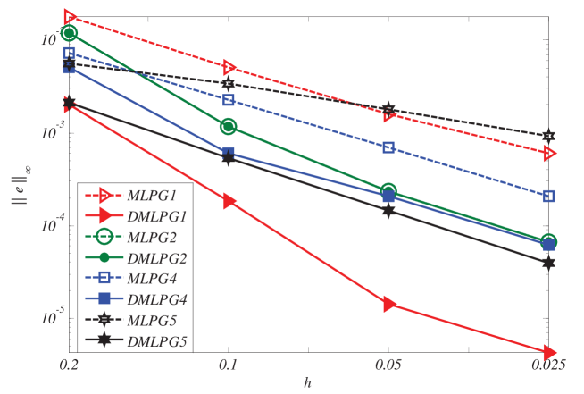
Figure 1: Comparison of MLPG and DMLPG methods in terms of maximum errors.

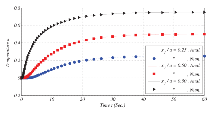
Figure 2: Time variation of the temperature at three positions with $\gamma=0$.

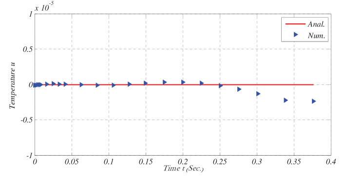
Figure 3: Accuracy of method for early time instants at position $x_{1}/a=0.5$.

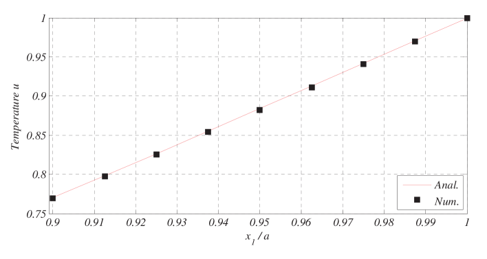
Figure 4: Accuracy of method for points close to the thermal shock at time $t(70)$ sec.

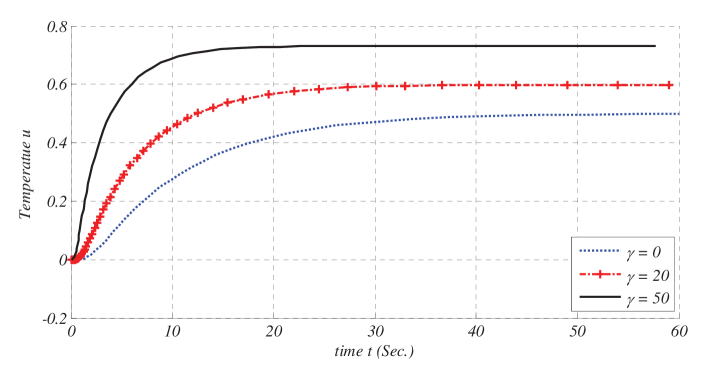
Figure 5: Time variation of the temperature at position $x_{1}/a=0.5$ for $\gamma=0,20,50$ m^-1.

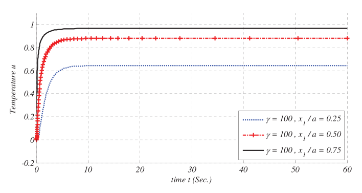
Figure 6: Time variation of the temperature at positions $x_{1}/a=0.25,0.5,0.75$ for $\gamma=100$ m^-1.

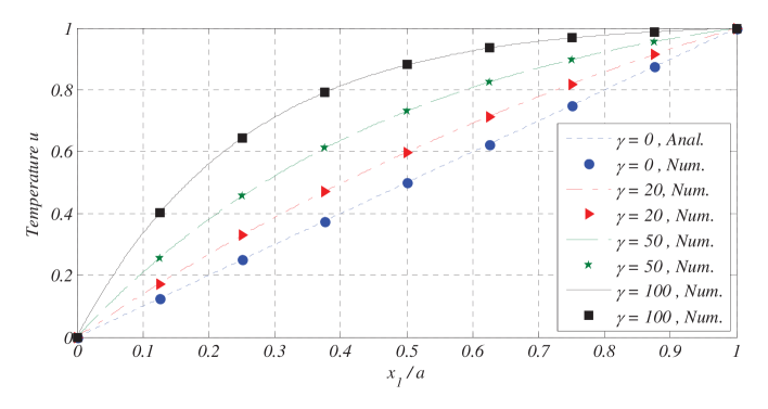
Figure 7: Distribution of temperature along $x_{1}$-axis under steady-state loading conditions.

References

- (1) S. N. Atluri, The meshless method (MLPG) for domain and BIE discretizations, Tech Science Press, Encino, CA, 2005.
- (2) I. Babuska, U. Banerjee, J. Osborn, Q. Zhang, Effect of numerical integration on meshless methods, Comput. Methods Appl. Mech. Engrg. 198 (2009) 27–40.
- (3) T. Belytschko, Y. Krongauz, D. Organ, M. Fleming, P. Krysl, Meshless methods: an overview and recent developments, Computer Methods in Applied Mechanics and Engineering, special issue 139 (1996) 3–47.
- (4) T. Belytschko, Y.Y. Lu, L. Gu, Element-Free Galerkin methods, Int. J. Numer. Methods Eng. 37 (1994) 229-256.
- (5) W.J. Minkowycz, E.M. Sparrow, G.E. Schneider, R.H. Pletcher, Handbook of Numerical Heat Transfer, John Wiley and Sons, Inc., (1998) NewYork,
- (6) D. Mirzaei, M. Dehghan, MLPG Method for Transient Heat Conduction Problem with MLS as Trial Approximation in Both Time and Space Domains, CMES–Computer Modeling in Engineering & Sciences, 72 (2011) 185-210.
- (7) D. Mirzaei, M. Dehghan, New implementation of MLBIE method for heat conduction analysis in functionally graded materials, Eng. Anal. Bound. Elem. 36 (2012) 511-519.
- (8) D. Mirzaei, R. Schaback, Direct Meshless Local Petrov-Galerkin (DMLPG) method: A generalized MLS approximation, Applied Numerical Mathematics, Inpress (2013), doi: 10.1016/j.apnum.2013.01.002.
- (9) D. Mirzaei, R. Schaback, M. Dehghan, On generalized moving least squares and diffuse derivatives, IMA J. Numer. Anal. 32, No. 3 (2012) 983–1000, doi: 10.1093/imanum/drr030.
- (10) J. Sladek, V. Sladek, S.N. Atluri, Meshless Local Petrov-Galerkin Method for Heat Conduction Problem in an Anisotropic Medium, CMES–Computer Modeling in Engineering & Sciences, 6 (2004) 309–318.
- (11) J. Sladek, V. Sladek, Ch. Hellmich, J. Eberhardsteiner, Heat conduction analysis of 3-D axisymmetric and anisotropic FGM bodies by meshless local Petrov-Galerkin method, Comput. Mech. 39 (2007) 223–233.
- (12) J. Sladek,V. Sladek, Ch. Zhang, Transient heat conduction analysis in functionally graded materials by the meshless local boundary integral equation method, Computational Materials Science, 28 (2003) 494–504.
- (13) J. Sladek, V. Sladek, M. Tanaka, Ch. Zhang, Transient heat conduction in anisotropic and functionally graded media by local integral equations, Eng. Anal. Bound. Elem. 29 (2005) 1047-1065.
- (14) H. Wang, Q.-H. Qin, Y.-L. Kang, A meshless model for transient heat conduction in functionally graded materials, Comput. Mech. 38 (2006) 51–60.
- (15) H. Wendland, Scattered Data Approximation, Cambridge University Press, 2005.
- (16) T. Zhu, J. Zhang, S. Atluri, A local boundary integral equation (LBIE) method in computational mechanics, and a meshless discretization approach, Comput. Mech. 21 (1998) 223–235.