Exclusion processes on networks as models for cytoskeletal transport

Abstract

We present a study of exclusion processes on networks as models for complex transport phenomena and in particular for active transport of motor proteins along the cytoskeleton. We argue that active transport processes on networks spontaneously develop density heterogeneities at various scales. These heterogeneities can be regulated through a variety of multi-scale factors, such as the interplay of exclusion interactions, the non-equilibrium nature of the transport process and the network topology.

We show how an effective rate approach allows to develop an understanding of the stationary state of transport processes through complex networks from the phase diagram of one single segment. For exclusion processes we rationalize that the stationary state can be classified in three qualitatively different regimes: a homogeneous phase as well as inhomogeneous network and segment phases.

In particular, we present here a study of the stationary state on networks of three paradigmatic models from non-equilibrium statistical physics: the totally asymmetric simple exclusion process, the partially asymmetric simple exclusion process and the totally asymmetric simple exclusion process with Langmuir kinetics. With these models we can interpolate between equilibrium (due to bi-directional motion along a network or infinite diffusion) and out-of-equilibrium active directed motion along a network. The study of these models sheds further light on the emergence of density heterogeneities in active phenomena.

1 Introduction

Over the last decades our knowledge on the composition and functioning of the cellular organelles has increased considerably [1], but understanding how cells self-organize and make their molecular components self-assemble into cellular compartments and structures is still a major challenge in cellular biology [2, 3]. How a cell works is undoubtedly related to its internal organization and the spatial distributions of its components on different scales. One may guess that order at mesoscopic scales is a consequence of the non-equilibrium nature of cellular processes. How self-organization arises spontaneously in non-equilibrium physics is also a a topic of current interest in non-equilibrium statistical physics, and is referred to as the study of active matter [4, 5].

Cells require active fluxes of matter to maintain their internal organization. To function properly cells thus need to establish a specific spatio-temporal organization of proteins, organelles, etc. Delivery of cargoes in eukaryotic cells is functional for biological processes and mainly realized using an active transport process based on motor proteins moving along cytoskeletal filaments [1, 6, 7]. In general, cytoskeletal filaments in cells form intracellular networks which act as macromolecular highways along which motor proteins can deliver cargoes to specific locations in cells. In nerve cells, for instance, proteins and membranes must be transported from the cell body to the synaptic terminal, a distance which can reach several meters. Besides their important role in transporting cargo, motor proteins have various other functions, e.g. force production leading to muscle contraction, depolymerization or rearrangement of the cytoskeletal filaments in cytoskeleton dynamics. Hence, the spatial organization of the motor proteins is an important aspect in the understanding of the physical and biological properties of cells. Motor-protein transport also has an important impact on the health of organisms: motor-protein mutations have been shown to lead to neurodegenerative diseases and they also play an important role in left-right body determination, tumour suppression, etc. [8, 9].

The physical picture of motor protein transport inside the cell is roughly the following. Motor proteins consume chemical energy at a high rate, which they employ to perform active motion along the polymer filaments of the cytoskeleton, in a preferential direction set by the filament polarity. These directed runs along the cytoskeleton typically alternate with diffusion in the cytoplasm, as the motors stochastically detach and re-attach via specific binding and unbinding processes. The distance which the motor protein typically moves between an attachment and a detachment event is a measure for its processivity (see for instance [10]). When motors reach a junction, where filaments branch or interconnect, they can change their direction or switch filament [11].

In recent years single motor protein motion has become experimentally observable due to progress in super-resolution imaging, physical manipulations of single molecules as well as electron and light microscopy. These have considerably boosted the ability to study the spatio-temporal organization of proteins within the cell. For instance, it is now possible to determine quantitatively, both in-vitro and in-cellulo, dynamic properties of single motor-proteins [12, 13, 14, 15], to quantitatively analyze the collective effects between interacting motors [16, 17], to observe the overall organization of proteins, organelles or membranes in the cell [18], as well as to present a 3D mapping of the topological structure of the cytoskeleton [19, 20, 21] and to control the formation of actin and microtubule networks of various topologies [22, 23]. It is a challenge to develop the modelling tools to complement the insights given by these experimental studies.

From a theoretical point of view, motor-protein transport is an intriguing example of a stochastic transport phenomenon of molecular entities, far from thermodynamic equilibrium and subject to mutual interactions. In statistical physics motor-protein transport is modelled by particles performing an active stochastic motion along a one-dimensional segment [24, 25, 26, 27]. One class of commonly used models are lattice gas exclusion processes, for which the particles are constrained in their movement by their excluded volume [28, 29, 30]. Their instantaneous velocities during the stepping process plays no role as such, since at the nanometer scale all motion is overdamped by the viscous environment. Active exclusion processes have been proposed originally in the context of mRNA translation by ribosomes [31, 32] and, more recently, have allowed to make quantitative predictions for in-vitro experiments on motor-protein transport along single filaments [17, 33, 34]. Thanks to extensive studies, we have now a rather in-depth understanding of non-equilibrium transport in a one-dimensional setting [35]. These lattice gas models have stimulated a lot of fundamental research in non-equilibrium physics [36], but also in more applied topics such as modelling macromolecules which move through capillary vessels [37], electrons hopping through a chain of quantum-dots [38], vehicular flow in traffic [39, 40], translation of mRNA [41]. Current studies have mainly focused on one-dimensional models, but they did not address how motor proteins spatially self-organize along the cytoskeleton.

Motor protein transport along the cytoskeleton can be envisaged as a generalisation of these processes to complex networks. Studies of transport processes on complex networks abound in the literature, starting from the seminal work of Kirchhoff on currents through electrical circuits [42]. Diffusion through networks is well-studied [43], and active transport processes through networks have been considered as models for motor protein transport [44, 45, 46, 47, 48, 49]. To date, most such models are mainly based on non-interacting particles. However, much interesting physics is expected when motors interact through exclusion interactions, and work on this aspect is recent. Greulich and Santen have studied particles moving actively on a spatially disordered network, also accounting for finite diffusion in the surrounding reservoir [50]. Ezaki and Nishinari have developed an exactly solvable model of an exclusion process on a network respecting a balance condition [51]. In our recent work [52, 53] we have shown that the stationary state of exclusion processes on complex networks can be understood in terms of their behaviour on a single-segment.

The role of heterogeneities has emerged from our previous studies as an important feature: since exclusion models in one dimension display a boundary-induced first-order phase transition in the particle density [54, 55], transport through complex networks leads to various regimes of density heterogeneities at different spatial scales [52, 53], which also depend on the network topology. We rationalize these phenomena starting from the transport characteristics of a single segment between two particle reservoirs. In particular, we build on the idea of effective rate diagrams which allow to visualize the stationary state of the network from the single-segment phase diagram [53]. Using this effective rate approach which we further develop in this article, we have identified three stationary regimes in exclusion models on networks, characterized by the spatial heterogeneities in the particle densities: a heterogeneous network regime, a heterogeneous segment regime and a homogeneous regime. We link these scales of heterogeneities to an interplay between the topology of the network, the microscopic (molecular) parameters for the transport process and the fraction of the network filled with particles. Our approach can be applied to any model for which the single-segment phase diagram and current density profiles through a single segment have been determined. Our approach is straightforwardly applicable to a large number of transport models for which the single-segment diagram is known [30, 35].

We apply our method to three different paradigmatic models: the totally asymmetric simple exclusion process (TASEP) [31, 32, 56], the partially asymmetric simple exclusion process (PASEP) [57] and the totally asymmetric simple exclusion process with Langmuir kinetics (TASEP-LK) [58, 59]. The TASEP is a model of active particles which hop stochastically and uni-directionally through a network and mutually interact with exclusion interactions. Interestingly, in recent work we have shown that transport through closed disordered networks by active particles following TASEP rules spontaneously leads to strong density heterogeneities between the different segments of the network [52]. To establish a clear understanding on how these heterogeneities appear in non-equilibrium transport processes we consider an extension of TASEP in two ways: we consider bi-directional motion of active particles on networks (PASEP) and the coupling of active motion through a network with the passive diffusion of particles in a reservoir (TASEP-LK). These extensions allow us to interpolate between a passive transport process (observed for fully bi-directional or diffusive motion) and an active transport process (for uni-directional motion along the network). In such a way we gain insight into the emergence of density heterogeneities on networks (which are absent in passive processes but appear in active processes). In the perspective of biological modelling, these models add important molecular parameters to the TASEP description of motor protein transport along the cytoskeleton.

In the following section we describe our general mathematical framework of active particles moving along complex networks, presented here in the perspective of motor protein transport along the cytoskeleton. We define the random networks and excluded volume processes which model, respectively, the cytoskeletal architecture and motor protein motion along the biofilaments. In the third section we introduce the two main concepts which allow us to intuitively understand and characterize the stationary state of excluded volume processes on networks: effective rate diagrams for the network and a classification of stationary states based on three regimes of particle density heterogeneities. We introduce these concepts first on TASEP, revisiting and extending the results presented in [52]. We then show in section four how this effective rate approach can be applied to understand bi-directional transport on networks and, in section five, to understand active transport on networks coupled to a homogeneous particle reservoir. The latter analysis considerably extends the results presented in [53]. The study of these three models shows how the stationary states of exclusion processes can be classified in a unified way using the three stationary regimes of density heterogeneities sketched above. We discuss the potential implications of our findings in the context of cytoskeletal motor protein transport using experimental values from the literature.

In the conclusions we summarize how this classification allows to present in a compact way how spatial density heterogeneities appear in active transport on networks through an interplay between network topology, disorder, bi-directionality and finite particle processivity.

2 Modelling motor-protein transport

In this section we present our general modelling framework to study transport along complex networks, with a view towards motor-protein transport on the cytoskeleton. Cells are hugely complex systems consisting of a variety of building blocks based on macromolecular assemblies such as proteins, filaments, membranes, organelles, etc. [1, 60, 61]. We use minimal models to capture some of the essential qualitative features of motor protein transport. These minimal models consist of particles (motor proteins) moving directionally along a graph (the cytoskeleton) as represented in figure 1.

Figure 1: (a) Microtubular network of a COS cell (courtesy of P. Montcourrier, CRLC Val d’Aurelle); (b) scheme of the microtubular network; (c) zoom on filaments with motor transport, binding and unbinding; (d) TASEP-LK microscopic rules for transport along a single filament.

2.1 Cytoskeleton as a directed network

The cytoskeletal meshwork of filaments is represented as a directed graph of segments of length $L$ which are interconnected at junction sites or vertices. A directed graph is a couple $G=(V,E)$ of the set of vertices $v\in V$ and directed edges or segments $s\in E\subset V\times V$. It is represented through nodes interlinked by arrows (see figures 1 and 2). In figure 2 the segments are represented as dashed lines and the junction sites as squares. This representation of the cytoskeleton as a directed network of segments takes into consideration the polarization of the cytoskeletal filaments, their discrete microscopic nature as well as the one-dimensional nature of the protofilaments.

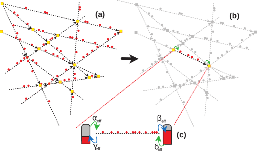
Figure 2: (a) Transport of particles along a network as a minimal model for cytoskeletal motor-protein driven transport; (b) The stationary state of the whole network can be studied by considering that every segment is an open segment which connects two reservoirs from the entrance of the segment towards the exit. (c) The two reservoirs are characterized by certain effective rates which depend on the state of the network, in particular the particle density at the junction nodes.

In principle we could consider a specific topology of the cytoskeletal network, as it may be known from experiments with cryo-electron tomography [20, 21] or from in-vitro reconstituted polymer networks using micropatterning methods [22, 23]. A static characterization of the cytoskeleton is however difficult, since the cytoskeleton is in fact a highly dynamic network due to e.g. (de)polymerization of filaments or (un)binding of cross-linker proteins. Moreover, due to the intrinsic complexity of the cytoskeleton, working on any particular structure would make it more difficult to unveil the main mechanisms leading to overall motor protein organization. In this perspective, theoretical studies are useful to explore the influence of any possible realization of a network topology on motor protein transport.

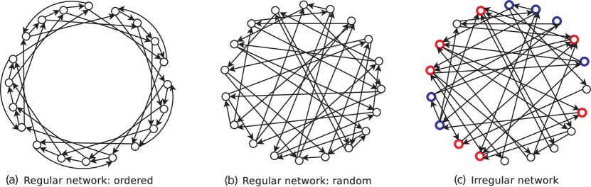
Figure 3: Three directed graphs which could serve as a model for the topology of a cytoskeleton. Left: ordered square lattice of degree $c=2$. Middle: 2-regular random graph. Although the local connectivities of the vertices are the same, disorder is present in how vertices are connected at long distances. Right: irregular random graph of mean connectivity $c=2$. In this case, the local neighbourhoods of vertices vary from site to site. We remark that the circles denote the junction sites while the crossings between segments do not represent real intersections. Red vertices have more incoming segments than outgoing ones, blue ones have more outgoing segments than incoming ones, and for black vertices the number of ingoing and outgoing segments is equal.

Here we consider random networks in which a single graph instance is drawn with a certain probability from an ensemble of graphs [62]. The randomness in the construction of the graph reflects to a certain extent our lack of knowledge in the precise cytoskeletal structure, as well as the complexity of the cytoskeleton. In this work we consider two types of graph ensembles: one without local disorder (the $c$-regular ensemble, a.k.a. Bethe lattice [63, 64]), and one with local disorder (the irregular Erdös-Rényi ensemble) [65, 66]. Local disorder is defined through disorder in vertex degrees. We define the indegree $c^{\rm in}_{v}$ of a vertex $v$ as the number of segments arriving at a vertex while the outdegree $c^{\rm out}_{v}$ denotes the number of segments leaving a vertex $v$. Regular graphs are then defined by the constraint $c^{\rm out}_{v}=c^{\rm in}_{v}=c$, such that all vertices have equivalent local neighbourhoods. As illustrated in figure 3, we can consider ordered regular graphs such as the square lattice or random regular graphs such as Bethe lattices. In irregular graphs the local vertex degrees of different vertices can differ, as in the Erdös-Rényi ensemble mentioned above. In this ensemble single graph instances are constructed by randomly drawing edges between the vertices: each directed segment of the graph is present with a probability $c/|V|$ and absent with a probability $1-c/|V|$. Networks drawn from the Erdös-Rényi ensemble have a Poissonian degree distribution. We select the strongly connected component of the graph [52, 67], whenever necessary, to make sure that every junction can be reached from every other junction.

As an illustration, we juxtapose in figure 3 the square lattice, as well as single graph instances drawn from the ensembles of regular and irregular graphs. These ensembles have been studied extensively in graph theory [62], and have been used to study complex networks appearing in various sciences, e.g. the Internet, social networks, regulatory networks in biology [68, 69].

2.2 Motor proteins as active particles

Motor protein motion through one cytoskeletal filament is modelled as a stochastic and biased motion through a single directed segment of the network, see figure 4. In this work we base the particle motion on one specific class of microscopic models known as exclusion processes. For these particles hop stochastically along the sites of the segments, with an excluded volume condition which forbids that several particles occupy the same site.

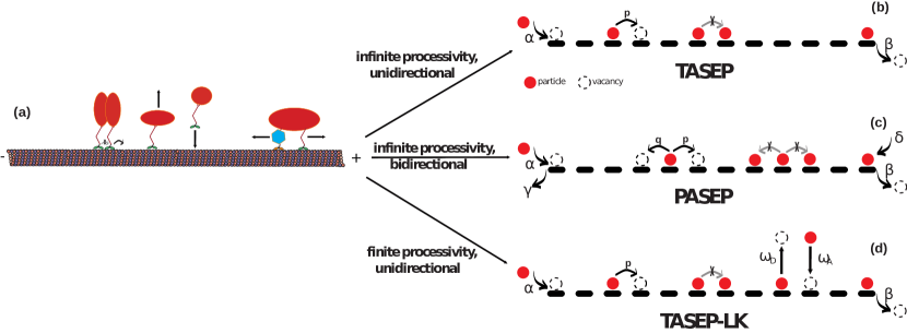
Figure 4: (a) Motor protein transport on a single filament: motors can stochastically step, without overtaking. They can bind and unbind in a kinetic exchange between the filament and the cytoplasm. In certain cases the motors, or cargoes driven by competing motors, may also undergo bi-directional motion. (b) TASEP process mimicking stochastic motion in one direction only, with site-exclusion and perfect processivity of motors. (c) PASEP process representing bi-directionality of motors or cargoes. (d) TASEP-LK reproducing unidirectional motion, but also binding and unbinding processes of motors.

There are several reasons why exclusion processes are good models to study motor protein transport on a mesoscopic level. First, they reduce many complex details of the stepping process to a rather simple set of rules. In particular they allow to study collective effects in active transport due to the interactions between the particles (which is more difficult to compute in more elaborate models of motor protein transport [24, 25]). Second, it has been shown that exclusion processes can describe both qualitatively and quantitatively the spatio-temporal organization of motor proteins along single biofilaments [33, 34, 17]. Third, they have been studied extensively over the last decades, in the one-dimensional configuration of an open segment, interconnecting two particle reservoirs with injection/extraction rates $(\alpha,\delta)$ and $(\gamma,\beta)$, respectively (see figures 4 and 2). At this moment, analytical expressions for the average current and density are known for numerous exclusion processes [30, 35], which will prove important when addressing generalizations to networks.

In figure 4 we illustrate three examples of exclusion models which retain some of the essential characteristics of motor protein transport. The simplest variant is the totally asymmetric simple exclusion process (TASEP), in which particles hop uni-directionally along a single segment at a fixed rate $p$ [31, 32, 56] (see figure 4-(b)). A simple extension of this model is given by the partially asymmetric simple exclusion process (PASEP) [57]. Here the forward rate $p$ and the backward rate $q$ differ (see figure 4-(c)). Such a generalization of TASEP is useful for capturing the bi-directional motion of motors, which can be due to fluctuations or to competing motors transporting a cargo. Finally we consider the totally asymmetric simple exclusion process with Langmuir kinetics (TASEP-LK). This model adds particle exchange with a reservoir, through a binding/unbinding process obeying Langmuir kinetics, to the TASEP model (see figure 4-(d)). Such exchange kinetics are important when studying active transport of motors with finite processivity, which can only cover a finite distance along the segment before they detach stochastically.

In the following we generalize the models presented in figure 4 to a complex network and study their stationary state. In terms of the dynamics on the network, we have to complement the above rules for particle hopping in the segments by a set of microscopic rules for their behavior at the junctions. A particle located at a junction site can jump to either of the outgoing segments with equal probability, and will then continue its one-dimensional dynamics along the new segment (see for instance figures 1 and 2). Here we consider the simplest choice, where jumps to all outgoing segments are equally likely, but other choices are possible [70, 71], to which our analysis could easily be adapted.

2.3 Balancing currents at the junctions and segment properties from effective rates

We present now a method to deduce the stationary density profiles of particles moving through a network from the stationary density profiles of an individual segment [52]. As illustrated in figure 2, we consider that the end points of every segment in the network connect to reservoirs which inject/extract particles with certain effective rates. The expressions of these rates are given, following mean-field arguments, by the occupation probabilities of the junction sites $v$, i.e. by the average density $\rho_{v}$ at the junctions. This allows us to develop a description of transport through a complex network for which the densities $\rho_{v}$ at the junction sites are sufficient to determine all the currents and densities in the whole network (even within the segments, since the junction densities determine the effective rates of each segment).

We determine the (average) densities $\rho_{v}$ by balancing currents at the junctions [52]. The continuity equations in $\rho_{v}$ read as:

$$\frac{\partial\rho_{v}}{\partial t}=\sum_{s\rightarrow v}J_{s\rightarrow v}-\sum_{s\leftarrow v}J_{v\rightarrow s}.$$ (1)

The quantity $J_{s\rightarrow v}$ is the average current of particles flowing from a segment $s$ into a junction site $v$, whereas $J_{s\leftarrow v}$ is the reverse flow from the junction $v$ into the segment $s$. Note that the sums in equation (1) run over the segments of the graph and therefore considers its specific topology.

We assume now that the particle current in any given segment $s=(v,v^{\prime})$ is given by the current between two particle reservoirs with appropriately chosen effective rates $(\alpha^{\rm eff}_{s},\delta^{\rm eff}_{s})$ and $(\beta^{\rm eff}_{s},\gamma^{\rm eff}_{s})$, see figure 2-(c). Hence the exact continuity equations (1) are approximated by the following mean-field equations

$$\frac{\partial\rho_{v}}{\partial t}=\sum_{s\rightarrow v}J^{-}\left[\alpha^{\rm eff}_{s},\delta^{\rm eff}_{s};\gamma^{\rm eff}_{s},\beta^{\rm eff}_{s}\right]-\sum_{s\leftarrow v}J^{+}\left[\alpha^{\rm eff}_{s},\delta^{\rm eff}_{s};\gamma^{\rm eff}_{s},\beta^{\rm eff}_{s}\right],$$ (2)

where $J^{-}$ and $J^{+}$, the current entering (leaving) the given segment, have the generic functional form known from a single segment: the in/out currents vary from one segment to the other only through the effective rates of the respective segments.

In the stationary state, closure of the set of equations (2) is achieved by establishing the expressions of the effective rates, for any segment $s=(v,v^{\prime})$, by linking them to the (average) junction densities $\rho_{v}$ and $\rho_{v^{\prime}}$. The appropriate expression for the effective rates can be found using a mean-field approximation at the junctions [70]. Note that even for those cases where the exact expression for the single-segment current is known, our procedure remains an approximation as segment cross-correlations at the junctions are not accounted for.

A particularly interesting aspect of our approach is that it constructs the description of transport at a network scale, from transport within the single segments. This leads to a strong simplification of the master equations, allowing to solve them on very large networks. Moreover, due to this decomposition one can apply our scheme to any model, with the sole condition of knowing a solution $J^{\pm}_{v}$ for a single open segment with entrance/exit rates $\left(\alpha,\delta\right)$ and $\left(\gamma,\beta\right)$. Since several non-equilibrium models for transport have been solved exactly in this particular one-dimensional configuration [30, 35], our approach is straightforwardly applicable to a very large number of models.

Let us finally define a certain number of macroscopic quantities which we will use throughout the article. The total density $\rho$ and the total current $J$ of the network are given by

$$\rho \equiv \frac{L\sum_{s\in S}\rho_{s}+\sum_{v\in V}\rho_{v}}{|S|L+|V|}\approx\frac{\sum_{s\in S}\rho_{s}}{|S|},$$ (3)

$$J \equiv \frac{L\sum_{s\in S}J_{s}+\sum_{v\in V}J_{v}}{|S|L+|V|}\approx\frac{\sum_{s\in S}J_{s}}{|S|}.$$ (4)

where the approximations are valid if individual segments are sufficiently long $(L\gg 1)$. The quantities $\rho_{s}$ and $J_{s}$ denote the average current and density through a given segment $s$. When strong heterogeneities appear in the network, it is particularly interesting to consider the distribution $W$ of segment densities $\rho_{s}$:

$$W(\rho_{s})\equiv|S|^{-1}\sum_{s\in S}\delta(\rho-\rho_{s}).$$ (5)

3 Analyzing TASEP on networks: effective rate diagrams and regimes of heterogeneity

In this section we introduce two concepts which will prove central for studying exclusion processes on networks: effective rate diagrams for the network and a classification of stationary states in terms of three regimes for heterogeneities. The effective rate diagrams provide an intuitive yet quantifiable method which allows to rationalize the stationary state of transport processes on networks in terms of their single segment phase diagram. One of the merits of this approach is a natural classification of the stationary state of exclusion processes on networks in terms of three distinct regimes: a heterogeneous network regime, a heterogeneous segment regime and a homogeneous regime. These regimes correspond with the different scales on which density heterogeneities can arise in the stationary state. As we will show in this work, these regimes give a unified view on the stationary state of exclusion processes on networks and allow to appreciate the effect of the network topology and of microscopic rules for particle motion.

Here we use TASEP on a network [52] to introduce these concepts. TASEP, illustrated in figure 4-(a), is the simplest model. Particles follow TASEP rules in each segment of the network. At the junction sites they hop, with equal probabilities, to one of the segments leaving the junction. The model thus consists of a closed network on which particles, at a given overall density $\rho$, move uni-directionally, stochastically and subject to mutual exclusion interactions.

Since the effective rate diagram builds on the single-segment phase diagram we first recapitulate the behavior of TASEP on a single open segment connecting two reservoirs (see the setting illustrated in figures 2-(c) and 4-(b)). We use the resulting current and density profiles to determine the spatial stationary distribution of particles along complex networks and discuss the classification in terms of the length scales associated with heterogeneities.

3.1 One-dimensional segment connecting two reservoirs

We recall the exact TASEP expressions for the current and density of particles moving through an open segment connecting two particle reservoirs, as shown in figure 2-(c), in the limit of large segments ($L\rightarrow\infty$). At the entrance particles are injected into the segment from a reservoir (with entry rate $\alpha$), whereas at the end of the segment they are absorbed into a reservoir (with exit rate $\beta$). In between particles hop uni-directionally at rate $p$ with mutual exclusion interactions, see figure 4-(b). The segment density as a function of the reservoir rates $(\alpha,\beta)$, is given by [56, 72, 55]:

$$\rho^{\rm TASEP}\left[\alpha,\beta\right]=\left\{\begin{array}[]{ccc}\alpha/p&\alpha<\beta,\ \alpha/p<1/2&\left({\rm LD}\right)\\ 1-\beta/p&\alpha>\beta,\ \beta/p<1/2&\left({\rm HD}\right)\\ 1/2&\alpha/p,\beta/p>1/2&\left({\rm MC}\right)\end{array}\right.,$$ (9)

and the average current $J$ obeys the parabolic profile:

$$J^{\rm TASEP}\left[\alpha,\beta\right]/p = \>\rho^{\rm TASEP}\left[\alpha,\beta\right]\left(1-\rho^{\rm TASEP}\left[\alpha,\beta\right]\right).$$ (10)

This average current is constant along a one-dimensional segment, since the particle number is conserved.

As one can see from equations (9), TASEP leads to three stationary phases: a low-density phase (LD) for low values of $\alpha$, a high-density phase (HD) at low values for $\beta$ and a maximal current phase (MC) if both $\alpha$ and $\beta$ are large. In the LD and HD phases the density and current profiles are boundary-controlled by the input or the exit rate, respectively. The maximal current phase (MC) on the other hand is a saturated, bulk-limited phase, invariably at density $\rho=1/2$ and with maximal current $J=p/4$. Note that in this MC phase the bulk density and current are independent of the boundaries.

The LD and HD phases are separated by a first order transition line at $\alpha=\beta<1/2$, where a coexistence phase (LD-HD) arises. Whereas the LD and HD phases correspond to homogeneous density profiles (except for localised boundary effects), the LD-HD phase is heterogeneous, as a domain wall separates the LD and HD regions which coexist on the same segment [73].

The first order transition separating LD and HD phases is an important feature when discussing transport on networks. It implies a discontinuous variation in density at $\alpha=\beta$, from the LD value $\rho_{LD}=\alpha/p$ to the HD value $\rho_{HD}=1-\beta/p$. The corresponding jump has size $\Delta\rho=\rho_{HD}-\rho_{LD}=1-2\alpha/p$, and we point out that it is maximal ($\Delta\rho=1$) at the origin. This observation will become important when analysing networks in the following subsections.

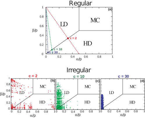
Figure 5: Effective rate diagram, obtained by mapping the steady state effective rates $(\alpha^{\rm eff}_{s}/p,\beta^{\rm eff}_{s}/p)$ for all segments $s$ in a network onto the single-segment phase diagram of TASEP [55, 56, 72]. The effective rates have been determined from the mean-field equations (12), and we have chosen an overall particle density $\rho=0.4$ for all cases shown (a): $c$-regular graph, at the given values of $c$. All effective rates of all segments are equal, and coincide in one data point, shown here for $\rho=0.4$. For other densities the effective rates $(\alpha^{\rm eff},\beta^{\rm eff})$ fall on the dashed lines. (b)-(d): strongly connected component of an irregular Erdös-Rényi graph, of given mean connectivity $c$. We have a scattered plot of effective rates, as these vary from segment to segment. The number of junctions in the graphs are: $|V|=155$ $(c=2)$, $|V|=200$ $(c=10)$ and $|V|=500$ $(c=30)$.

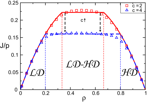
Figure 6: Average current-density relation through regular graphs for a given degree of connectivity $c$. The plateau indicates the presence of a first order transition and a coexistence phase, which dominates at increasing connectivities. The dashed lines indicate the transitions between the homogeneous $\mathcal{LD}$ region, the heterogeneous $\mathcal{LD-HD}$ segment region and the homogeneous $\mathcal{HD}$ region. Simulations (markers) are for segments of length $L=100$ and graphs of size $|V|=80$ junctions. The agreement between mean-field profiles (solid lines) and simulations improves further when increasing the segment length $L$.

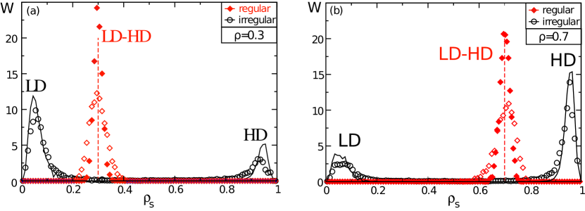
Figure 7: The distributions $W$ of the segment densities $\rho_{s}$ for regular and irregular networks are compared for two graph instances of average connectivity $c=10$. Note the difference between the bimodal distribution for irregular graphs and the unimodal distribution for regular graphs. We compare mean-field results (lines) with simulation (markers). The total density $\rho$ equals $\rho=0.3$ (a) and $\rho=0.7$ (b). The graphs have a size of $|V|=1000$ junctions. Simulations are run for segments of length $L=100$. The unimodal distribution of regular graphs predicted by mean-field is approached gradually by simulations when increasing the runtime.

3.2 Effective rate diagrams describing TASEP through a network

To determine the stationary distribution of particle densities for the TASEP on networks we apply the mean-field analysis laid out in subsection 2.3. The current and density profiles for an individual segment $s$ in the network, $J_{s}$ and $\rho_{s}$, are given by $J_{s}=J^{\rm TASEP}\left[\alpha^{\rm eff}_{s},\beta^{\rm eff}_{s}\right]$ and $\rho_{s}=\rho^{\rm TASEP}\left[\alpha^{\rm eff}_{s},\beta^{\rm eff}_{s}\right]$. The incoming and outgoing currents in each segment must match: $J^{-}[\alpha,\beta]=J^{+}[\alpha,\beta]=J^{\rm TASEP}[\alpha,\beta]$, due to current conservation along a single segment. Equations (2) for TASEP are now closed by relating the effective rates $\alpha^{\rm eff}_{s}[\rho_{v}]$ and $\beta^{\rm eff}_{s}[\rho_{v^{\prime}}]$ for each segment $s=(v,v^{\prime})$ in the network to the junction densities $\left\{\rho_{v}\right\}_{v\in V}$. From the microscopic behaviour of the particles at the junctions, here the excluded volume and the fact that all out-junctions are selected with equal probability, mean-field arguments lead to [70]:

$$\alpha^{\rm eff}_{v}=p\frac{\rho_{v}}{c^{\rm out}_{v}}\qquad\mbox{and}\qquad\beta^{\rm eff}_{v}=p\left(1-\rho_{v}\right),$$ (11)

where $c^{\rm out}_{v}$ is the out-degree of junction $v$, i.e. its number of outgoing segments.

Substituting the effective rates in equations (2) leads to the following set of closed equations in the density at the junctions $\rho_{v}$:

$$\frac{\partial}{\partial t}\rho_{v}=\sum_{v^{\prime}\rightarrow v}J^{\rm TASEP}\left[p\frac{\rho_{v^{\prime}}}{c^{\rm out}_{v^{\prime}}},p\left(1-\rho_{v}\right)\right]-\sum_{v^{\prime\prime}\leftarrow v}J^{\rm TASEP}\left[p\frac{\rho_{v}}{c^{\rm out}_{v}},p\left(1-\rho_{v^{\prime\prime}}\right)\right].$$ (12)

Solving this set of equations, analytically or numerically, one finds stationary values for the densities at the junctions $\left\{\rho_{v}\right\}_{v\in V}$, which determine the stationary state of the network. These densities imply the effective rates $(\alpha^{\rm eff}_{s},\beta^{\rm eff}_{s})$ for each segment, and thus also the average segment densities $\rho_{s}$ as well as the average currents $J_{s}$ through each segment $s\in S$ (see equations (9)-(10)).

A very useful way to visualize and understand the transport characteristics of a network is achieved by mapping the effective rates of the segments in the network onto the $(\alpha/p,\beta/p)$-phase diagram of a one-dimensional open segment, see figure 5. The state of the whole network can thus be visualized by an effective rate diagram, represented in figure 5, from which one can read off which phases are occupied by the segments in the network. We notice a striking difference between the stationary state of regular networks, for which all segments fall into the same phase, and irregular networks, for which the effective rates are scattered over the single-segment phase diagram. We discuss in the next two paragraphs how this sets apart regular from irregular networks.

3.3 Regular networks

For regular networks all junctions are topologically identical, which also makes all segments identical. Consequently all transport is governed by one pair of effective rates, and ultimately (from equation (11)) by a single value for the junction occupancy $\rho_{v}$. The latter depends on the overall density $\rho$, and the dashed lines in Figure 5-(a) show how the effective rates evolve as the overall density $\rho$ varies. The labeled points correspond to an overall density of $\rho=0.4$, and here they fall onto the first order phase transition line, corresponding to a junction occupancy of $\rho_{v}=c/(c+1)$. Note that, due to the presence of phase coexistence, this value of the junction occupancy corresponds to a whole range of overall densities: $\rho\in[\rho^{\ast},1-\rho^{\ast}]$, with $\rho^{\ast}=(c+1)^{-1}$. This degeneracy is also reflected in the current-density relation $J(\rho)$ [70], which is identical to that of each segment in the network (see Fig. 6). The density heterogeneities associated with the LD-HD coexistence phase are directly linked to a drop in transport capacity, which leads to the current plateau.

In terms of the network, the conclusion is that at low densities ($\rho\leq\rho^{\ast}$) all segments are in the LD phase and the particles distribute homogeneously throughout the whole network. Similarly, at high densities ($\rho\geq 1-\rho^{\ast}$) all segments are in the HD phase. On the network level we refer to these as the homogeneous ($\mathcal{LD}$ or $\mathcal{HD}$) regimes, according to which phase dominates the behavior of the network. We reserve calligraphic letters to refer to the regimes of the network while the phases of the individual segments are denoted by regular letters. In contrast, at intermediate densities all segments are in the LD-HD coexistence phase, and thus heterogeneities are present within each of the segments. We refer to this as a heterogeneous $\mathcal{LD-HD}$ segment regime, to indicate that the density heterogeneities arise at the scale of single segments.

These characteristics are further illustrated in figure 7 where we present the distribution $W$ of segment densities $\rho_{s}$, here superposing results from numerically solving the mean-field equations and kinetic Monte Carlo simulations. There is good agreement for the irregular network. For a regular network the above mean-field arguments would predict a delta-peak at the overall density, here $\rho=0.3(\rho=0.7)$, since all segments behave identically. The simulations corraborate this for intermediate densities, in that we indeed observe a single peak, which corresponds to segments in the LD-HD phase. Data for two different simulation run lengths furthermore illustrate that the finite width of the peak reduces with the run length. Convergence to an actual Dirac distribution would require exceedingly long simulations, due to the presence of slow collective fluctuations in the coexistence phase [73].

3.4 Irregular networks

In irregular networks the phenomenology is drastically different. Here, as shown in figure 5-(b), the variation in local connectivity at the junctions makes the $(\alpha^{\rm eff}_{s},\beta^{\rm eff}_{s})$-effective rates scatter, such that certain segments are found in a LD phase whereas others are in a HD phase. Since the single-segment phase diagram of TASEP separates LD and HD phases by a first-order transition line ($\alpha=\beta<1/2$), the segment densities on an irregular network are bimodally distributed. Such bimodality is a signature of strong heterogeneities in the way particles are distributed on a network scale. We say that irregular networks show a $\mathcal{LD/HD}$ heterogeneous network regime.

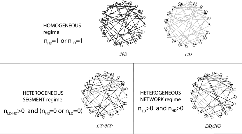
Figure 8: The stationary states of excluded volume processes on networks are classified in three distinct regimes. These correspond with the scale at which heterogeneities in the particle densities arise throughout the network. They are defined in terms of the fraction $n_{\rm HD}$, $n_{\rm LD}$ and $n_{\rm LD-HD}$ of segments which fall into the corresponding phases in the single-segment phase diagram, see figure 5. The MC phase will play a minor role in the following and therefore, for clarity, is not considered.

We quantify the above statements using the distribution of segment densities $W(\rho_{s})$ in figure 7. We indeed notice the appearance of two peaks in the distribution $W$: one peak is at low densities and accounts for the segments in the LD phase, whereas the other peak is at high densities and accounts for segments in the HD phase. As particles are added to the network the HD peak grows at the expense of the LD peak, reflecting that the segments successively switch from LD to HD phases. This can be visualized rather intuitively in the effective rate diagram 5 as the process of certain points crossing the coexistence line.

The high connectivity limit allows particularly well to pinpoint the role of heterogeneities in irregular networks. Intuitively, this limit corresponds to the case where all junctions become bottlenecks, thus reducing the flow of particles to almost zero. This is indeed apparent from the effective rates, which scale as $c$ as $(\alpha^{\rm eff},\beta^{\rm eff})\sim(\mathcal{O}(c^{-1}),\mathcal{O}(c^{-1}))$, see analytical arguments in the supplemental material of [52]. As a consequence they cluster in the $(\alpha,\beta)$-phase plane in a zone which progressively retracts to the origin as $c$ increases, see figure 5-(b). Since this zone includes the first order transition lines we not only preserve the bimodality in the high connectivity limit, but heterogeneities become even more pronounced, given that the density discontinuity associated with the LD to HD transition is maximum at the origin.

3.5 Discussion: three stationary regimes two classify density heterogeneities

Counterintuitive non-equilibrium phenomena, such as the emergence of strong density heterogeneities in active transport on networks, can be clearly understood using effective rate diagrams as presented in figure 5. In particular, it appears natural to classify the stationary behaviour using three different regimes. They are defined based on the fractions $n_{\rm LD}$, $n_{\rm HD}$, $n_{\rm LD-HD}$ of segments which occupy the corresponding phases in the effective rate diagrams:

• heterogeneous network regime ($\mathcal{LD/HD}$): a finite fraction of segments occupy the LD phase and a finite fraction occupies the HD phase. We thus have that both $n_{\rm LD}>0$ and $n_{\rm HD}>0$. The distribution of segment densities $W(\rho_{s})$ is bimodal, with a LD peak at low densities and a HD peak at high densities. As a consequence strong density heterogeneities develop on a network scale, i.e. between individual segments. At the same time LD and HD segments dominate, and the density profiles within single segments remain mostly homogeneous.

• heterogeneous segment regime ($\mathcal{LD-HD}$): the segments occupying the LD-HD phase dominate, and depending on the overall density either the LD or the HD phases are essentially unpopulated. We therefore have $n_{\rm LD-HD}>0$ and either $n_{\rm HD}=0$ or $n_{\rm LD}=0$. At the network scale transport thus behaves rather uniformly: the segment density distribution $W(\rho_{s})$ in the stationary state is dominated by a single peak corresponding to segments in LD-HD coexistence. The segments therefore behave similarly throughout the network, but strong heterogeneities are present within the segments due to LD-HD phase coexistence.

• homogeneous regime ($\mathcal{LD}$) or ($\mathcal{HD}$): all segments occupy either the LD, or HD phase, such that either $n_{\rm LD}=1$ or $n_{\rm HD}=1$. Particles are distributed homogeneously throughout the network and few heterogeneities appear at any scale.

The three regimes are visualized in figure 8. Again calligraphic letters systematically stand for the regimes of the entire network, rather than the phases of the segments.

The above observations highlight how the network topology affects density heterogeneities in TASEP transport. Regular networks lead to a $\mathcal{LD}$ homogeneous regime (at low densities), a $\mathcal{LD-HD}$ segment regime (at intermediate densities) and a $\mathcal{HD}$ homogeneous regime (at high densities). Irregular networks on the other hand are dominated by the $\mathcal{LD/HD}$ network regime in which homogeneous LD and HD segments coexist on the network level. This can easily be understood from the effective rate diagrams (figure 5). In this picture the strong heterogeneities in irregular networks is seen to be due to a combination of (i) the disorder in the effective rates and (ii) the first order transition in the single-segment phase diagram. This argument implies that heterogeneities must be expected to arise rather generally in excluded volume processes on networks: whenever the junctions in the network are subject to some sort of local disorder, effective rates will be scattered on the single segment phase diagram. The presence of a first order transition in the phase diagram then implies strong heterogeneities, since a fraction of the effective rates will fall into the LD part while others fall into the HD zones of the phase diagram. Based on these observations we can anticipate what will happen when generalizing other models to complex networks. Indeed, the first order transition around the origin is also present in models of TASEP with extended particles [74, 75], TASEP with syncrhonuous dynamics [76], TASEP with multiple lanes [77, 78, 79, 80], TASEP with particles with internal states [33, 81], TASEP with directional switching [82], etc. which suggests that they too will lead to strong network heterogeneities on disordered graphs. From this argument it also becomes clear that those strong heterogeneities do not depend on the particular choice of Erdös-Rényi networks we have considered here to model topological disorder. Rather, our results are expected to remain valid for other disordered systems such as scale-free networks, regular networks with disorder in the hopping rates at the junctions, etc.

4 Bi-directional transport of infinitely processive particles

In this work we intend to explore to which extent the microscopic motion of motors affects the presence of density heterogeneities in transport processes on networks. A closer look at the motion of motor proteins and their cargoes reveals that they can execute bi-directional moves along the bio-filaments. This may be due to backstepping of individual motors (known to account, for instance, for something like $2-10\%$ of the displacements in kinesin [83, 84, 85]), or to collective effects between motors of opposite polarity (e.g. for the transport of organelles [86, 87]).

We use PASEP to address the question of bi-directionality. In PASEP particles move in a preferential direction, but can also perform reverse hops, at a reduced rate, see figure 4-(c). TASEP is the special case where the rate for backward hopping is set to zero, whereas the opposite ’symmetric’ limit of equal backward and forward hopping corresponds to the symmetric exclusion process (SEP).

On networks we generalise SEP such that the symmetric limit ensures a homogeneous equilibrium distribution of particles throughout the network. TASEP on the other hand has been seen to provoke strong inhomogeneities. In the following we use PASEP to interpolate between an active and a passive process, in order to investigate to which extent the bi-directionality of microscopic motion affects the formation of large-scale density heterogeneities in the stationary state.

We follow the same outline as in the previous section. First we recapitulate the macroscopic behaviour of PASEP on a single open segment. In subsection 4.2 we use the resulting single-segment transport characteristics to determine the transport features through a large network. In the following subsections we explore the effect of connectivity on the transport features through a study of PASEP through regular and irregular networks. At last we discuss how heterogeneities disappear on networks when the PASEP process approaches the equilibrium limit.

4.1 Partially asymmetric exclusion process on a single segment

We revisit the transport characteristics of PASEP through a single, infinitely long segment connecting two reservoirs [57]. Particles are injected (extracted) with rates $\alpha(\gamma)$ on the left of the segment, and with rates $\delta(\beta)$ on the right, see figure 4-(c). In between particles hop forward (from left to right) at rate $p$, and they hop backwards at rate $q$. Just as in TASEP the particles interact through exclusion interactions. When we set $q=0$ we recover TASEP, while for $q=p$ this process reduces to the SEP.

The average current in PASEP must be constant throughout the segment, as particles can neither be destroyed nor created. Its current-density profile is parabolic, as is usual for exclusion processes:

$$J^{\rm PASEP}\left[\alpha,\gamma;\delta,\beta\right]=(p-q)\rho^{\rm PASEP}\left[\alpha,\gamma;\delta,\beta\right]\left(1-\rho^{\rm PASEP}\left[\alpha,\gamma;\delta,\beta\right]\right),$$ (13)

with a homogeneous density $\rho^{\rm PASEP}$

$$\rho^{\rm PASEP}\left[\alpha,\gamma;\delta,\beta\right]=\left\{\begin{array}[]{ccccc}\frac{(p-q+\gamma+\alpha)-\sqrt{(p-q+\gamma+\alpha)^{2}-4(p-q)\alpha}}{2(p-q)}&&\kappa[\alpha,\gamma]>\kappa[\beta,\delta],\kappa[\alpha,\gamma]>1,&&\mbox{(LD)}\\ \frac{(p-q-\beta-\delta)+\sqrt{(p-q-\beta-\delta)^{2}+4(p-q)\delta}}{2(p-q)}&&\kappa[\beta,\delta]>\kappa[\alpha,\gamma],\kappa[\beta,\delta]>1,&&\mbox{(HD)}\\ 1/2&&\kappa[\beta,\delta]\leq 1,\kappa[\alpha,\gamma]\leq 1.&&\mbox{(MC)}\end{array}\right.$$ (17)

(18)

Here we have assumed $q<p$, without any loss of generality, and taken the limit of infinite segment length ($L\rightarrow\infty$). The opposite case of $p<q$ is implicitly treated through particle-hole symmetry. The quantity $\kappa$ is a dimensionless function,

$$\kappa\left[\alpha,\gamma\right]=\frac{1}{2\alpha}\left(-\alpha+\gamma+p-q+\sqrt{(-\alpha+\gamma+p-q)^{2}+4\alpha\gamma}\right),$$ (19)

which will be central to the following discussion. We use the inverse quantities $\kappa^{-1}$, which allows us to cast the single-segment phase diagram into a familiar shape. The phase diagram maps directly onto that for TASEP, based on the quantites$\kappa[\alpha,\gamma]$ and $\kappa[\beta,\delta]$ introduced above, see figure 9) [57].

The PASEP has, just like TASEP, a first-order transition between an LD and a HD phase, along the coexistence line $\kappa\left[\alpha,\gamma\right]=\kappa\left[\beta,\delta\right]<1$. Since the position of this first order transition in the phase diagram was the key to our understanding of heterogeneities in TASEP on networks (limit $q=0$), it is now interesting to see how this picture is modified as particles are allowed to backstep ($q>0$). We find that the first order transition remains present, even in the limit of symmetric motion ($q\rightarrow p$). The density jump is equal to $\Delta\rho=\rho_{HD}-\rho_{LD}=1/(1+\kappa^{-1}\left[\beta,\delta\right])-1/(1+\kappa\left[\alpha,\gamma\right])$. Just as for TASEP this discontinuity increases when approaching the origin of the $(\kappa^{-1}\left[\alpha,\gamma\right],\kappa^{-1}\left[\beta,\delta\right])$-phase plane, and reaches its maximal value $\Delta\rho=1$ at the origin.

The TASEP limit ($q\rightarrow 0$) is straightforward: equation (18) reduces to $\kappa[\alpha,\gamma]=\alpha/(1+\alpha)$ and we recover the phase diagram of TASEP. In contrast, the symmetric limit $q\rightarrow p$ is more subtle: the limiting process is a SEP, but we do not recover the corresponding density profile from equations (18) when setting $q=p$: we find a homogeneous bulk density, determined by one of the two boundaries, whereas the SEP leads to a constant density gradient, $\rho_{LD}=\frac{\alpha}{\alpha+\gamma}$ and $\rho_{HD}=\frac{\delta}{\beta+\delta}$. The reason is that the limits $L\rightarrow\infty$ and $q/p\rightarrow 1$ do not commute. Since in equation (18) we have taken the limit $L\rightarrow\infty$ before considering $q/p\rightarrow 1$, the behaviour remains in the strongly asymmetric case [36]. We will return to this point when discussing networks in the following sections.

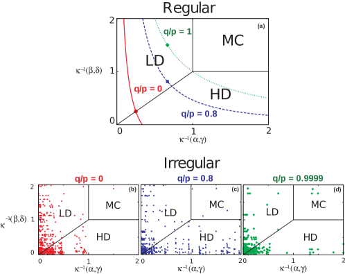
Figure 9: The effective rates for all segments of a given graph instance of mean connectivity $c=4$, mapped onto the $(\kappa^{-1}\left[\beta,\delta\right],\kappa^{-1}\left[\alpha,\gamma\right])$ phase diagram of a single open PASEP segment. The ratios of backward to forward hopping rates $q/p$ are indicated. The total density is $\rho=0.4$ in all examples, to facilitate comparison. (a): Effective rates (markers) for a regular network. The lines represent the relation between $\kappa^{-1}\left[\beta,\delta\right]$ and $\kappa^{-1}\left[\alpha,\gamma\right]$ when varying the total density $\rho$. (b)-(d): Effective rates for an irregular network of size $|V|=193$, for several ratios $q/p$. The diagrams are truncated at $\kappa^{-1}=2$, but data points are present over a larger range.

4.2 Effective rate diagrams for PASEP on networks

We base our study of PASEP transport on networks using the mean-field algorithm given by equations (2), as we did for TASEP in subsection 3.2. The current through a segment, $J_{s}=J^{\rm PASEP}\left[\alpha^{\rm eff}_{s},\gamma^{\rm eff}_{s};\delta^{\rm eff}_{s},\beta^{\rm eff}_{s}\right]$, is now given by equations (13)-(18). From current conservation we still have $J^{+}_{s}=J^{-}_{s}=J^{\rm PASEP}\left(\alpha^{\rm eff}_{s},\gamma^{\rm eff}_{s};\delta^{\rm eff}_{s},\beta^{\rm eff}_{s}\right)$. To determine the effective rates required to close the set of equations (2) we adopt the rule that particles which leave a junction select any of the outgoing segments with equal probability. In this way we obtain:

$$\alpha^{\rm eff}_{(v,v^{\prime})} = p^{{\rm junction}}_{v}\>\rho_{v},$$ (20)

$$\beta^{\rm eff}_{(v,v^{\prime})} = p\,(1-\rho_{v^{\prime}}),$$ (21)

$$\gamma^{\rm eff}_{(v,v^{\prime})} = q\,(1-\rho_{v}),$$ (22)

$$\delta^{\rm eff}_{(v,v^{\prime})} = q^{{\rm junction}}_{v^{\prime}}\>\rho_{v^{\prime}}.$$ (23)

The microscopic rates $p^{\rm junction}_{v}$ and $q^{\rm junction}_{v^{\prime}}$ denote the rates for particles at the junction site, i.e. $p^{\rm junction}_{v}$ is the rate for a particle on a junction to step into one of its $c^{\rm out}_{v}$ outgoing segments, whereas $q^{\rm junction}_{v^{\prime}}$ is the rate at which it backstpdf into one of the $c^{\rm in}_{v^{\prime}}$ incoming segments. We furthermore require the activity of particles at the junctions to be equal to the activity in the segments, i.e. $p+q=c^{\rm out}_{v}\>p^{{\rm junction}}_{v}+c^{\rm in}_{v}q^{\rm junction}_{v}$. Moreover, for $q=0$ we wish to recover TASEP rates ($q^{{\rm junction}}_{v^{\prime}}=0$, $p^{{\rm junction}}_{v}=p/c^{\rm out}_{v}$), whereas for $q=p$ we impose that the dynamics fulfill detailed balance, i.e. $p^{{\rm junction}}_{v}=q^{\rm junction}_{v^{\prime}}$. Considering the above conditions, we are lead to:

$$\alpha^{\rm eff}_{(v,v^{\prime})} = p\left(\frac{\rho_{v}}{\left(\frac{p}{p+q}\right)c^{\rm out}_{v}+\left(\frac{q}{p+q}\right)c^{\rm in}_{v}}\right),$$ (24)

$$\delta^{\rm eff}_{(v,v^{\prime})} = q\left(\frac{\rho_{v^{\prime}}}{\left(\frac{p}{p+q}\right)c^{\rm out}_{v^{\prime}}+\left(\frac{q}{p+q}\right)c^{\rm in}_{v^{\prime}}}\right).$$ (25)

Substituting these effective rates and the current profile equations (13) and (18) in the expression (2) leads to the required closed set of equations in the junction densities $\rho_{v}$. Note that due to our microscopic hopping rules at the junctions the the symmetric limiting process (q=p, corresponding to SEP) fulfills detailed balance, which leads to a stationary state with a completely homogeneous distribution of particles over the network.

It again proves insightful to map the effective rates of the segments onto the single-segment phase diagram of an open PASEP segment, via $\kappa^{-1}\left[\alpha^{\rm eff}_{s},\gamma^{\rm eff}_{s}\right]$ and $\kappa^{-1}\left[\beta^{\rm eff}_{s},\delta^{\rm eff}_{s}\right]$ for each segment $s\in S$. In figure 9 we compare the effective rate diagrams for a regular network (top) and an irregular network (bottom), for various ratios $q/p$. Note the similarity between the PASEP effective rate diagrams figures 9 and the TASEP effective rate diagrams figures 5.

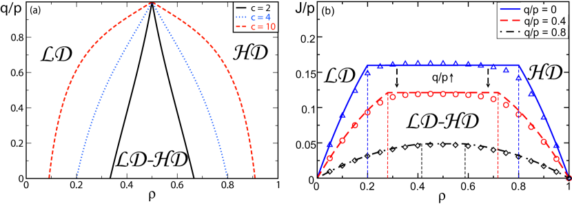
Figure 10: PASEP through regular graphs. Left (a): The transition lines between the $\mathcal{LD}$ and $\mathcal{LD-HD}$ regimes, as well as, the $\mathcal{LD-HD}$ and $\mathcal{HD}$ regimes are presented as a function of the total particle density $\rho$ and the fraction of rates $q/p$ for regular graphs of given degree $c$. For $q/p\rightarrow 1$ the process becomes passive. The heterogeneous $\mathcal{LD-HD}$ segment regime disappears in this limit. Right (b): Average current-density profile through regular graphs of degree $c=4$. The onset of a $\mathcal{LD-HD}$ regime is identified by a plateau in the current density profile. Mean-field results (solid lines) are compared with simulation results (markers) on graphs of $|V|=80$ junctions and segments of length $L=400$ at different degrees of particle asymmetry $q/p$. We have verified that deviations between mean field and simulations decrease with increasing segment size.

4.3 Regular networks

From the effective rate diagram in figure 9 we see that all segments have the same transport characteristics. Indeed, equations (2) admit the solution $\rho_{v}=\rho^{\prime},\ \forall v\in V$, i.e. an identical density on all vertices $v$. Thus all segments will have the same average current $J_{s}=J$ and average density $\rho_{s}=\rho$. The current-density profile for the network is therefore the truncated parabola of a single segment and the density at the junction is $\rho_{v}=c/(c+1)$ on the plateau.

This shows that, all in all, PASEP through regular networks leads to a stationary state similar to that of TASEP. At densities below those leading to coexistence in single segments ($\rho<\rho^{\ast}$) the network displays a homogeneous $\mathcal{LD}$ regime. At intermediate densities the system is in the heterogeneous $\mathcal{LD-HD}$ segment regime, while at high densities ($\rho>1-\rho^{\ast}$) we have the $\mathcal{HD}$ homogeneous regime. The segment regime corresponds to the plateau region in the current-density profile. Just as for TASEP the density range for the segment regime, of width $1-2\rho^{\ast}$, increases as a function of the connectivity $c$. On the other hand, the size of the segment regime gradually decreases to zero when approaching the symmetric $q=p$ limit corresponding to a passive process. Density heterogeneities thus disappear in this limit, see figure 10-(a).

We present the analytical mean-field solution for the current-density profile $J(\rho)$ of the network in figure 10-(b). The total density value $\rho^{\ast}$ separating the $\mathcal{LD-HD}$ segment regime and the homogeneous $\mathcal{LD}$ regime is given by

$$\rho^{\ast} = \frac{p-q+\frac{p+q}{c+1}-\sqrt{\left(p-q+\frac{p+q}{c+1}\right)^{2}-\frac{4(p-q)p}{c+1}}}{2(p-q)}.$$ (26)

In figure 10-(a) we have plotted this threshold $\rho^{\ast}$ as a function of $q$ and $p$ for various values of connectivity $c$. This constitutes the phase diagram for PASEP through regular networks. Note how the heterogeneities gradually disappear as the symmetric $q=p$ process is approached.

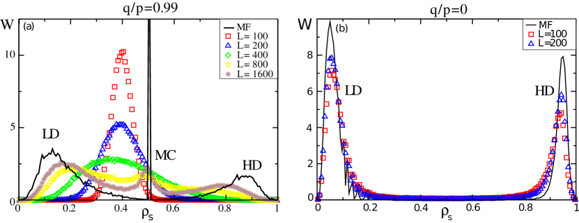
Figure 11: The distribution $W$ of the segment densities $\rho_{s}$ for a PASEP process on irregular networks at a total density $\rho=0.4$. We have plotted the average distribution over $100$ graph instances drawn from the Erdös-Rényi ensemble at mean connectivity $c=10$ and size $|V|=200$. Solid lines denote mean-field results while markers denote simulation results for indicated segment lengths $L$. Left (a): the almost symmetric $q/p=0.99$ case. We notice that for low values of $L$ the segment distribution is unimodal, peaked at the average value $\rho=0.4$. We are in a regime similar to passive diffusion. For larger values of $L$ we enter the active regime and trimodality arises in the segment distribution $W$ (the trimodality corresponds with the three phases: LD, HD and MC). The distribution seems eventually to converge to the mean-field expression. Right (b): We show how $W$ depends on $L$ in the totally asymmetric $q=0$ case. We see that the bimodality is already present at very low values of the segment lengths $L$.

4.4 Irregular networks

For irregular graphs the effective rate diagrams again show scatter plots, see figure 9. As a consequence, a finite fraction of segments will occupy the LD, HD and MC phases. Accordingly, the segment density distribution now displays three peaks corresponding to these three phases, see figure 11-(a). Note also that the peak associated with the MC phase gradually disappears in the TASEP limit ($q/p\rightarrow 0$). We expect this feature to change when considering a non-uniform hopping rule at the junctions.

Just as for regular graphs, it is possible to determine the overall network phase diagram for a PASEP process through an irregular graph (see figure 12). We use the definitions in figure 8 and in the discussion 3.5 to find the transition lines between the $\mathcal{LD/HD}$ and $\mathcal{LD}$ or $\mathcal{HD}$ phases on the network. Remarkably, we notice that the $\mathcal{LD/HD}$ network regime remains prominent, even for the symmetric limit $q\rightarrow p$.

This symmetric limit is a point worth discussing in the context of irregular networks. In principle we expect density heterogeneities to disappear in this limit, since we reach a passive equilibrium process. However, rather surprisingly, one can see from figure 11 that our mean-field results show a pronounced trimodality at values very close to this limit (here $q=0.99\>p$), suggesting that the trimodality persists even for $q=p$. This too can be understood from the effective rate diagram, since the first order transition in this diagram remains present in the symmetric limit (see figure 9). At first sight this result seems to contradict the fact that passive processes must lead to a homogeneous distribution of particles along the network. The reason for this apparent contradiction is the subtle interplay between the two limits $q\rightarrow p$ and $L\rightarrow\infty$ which do not commute, as mentioned in subsection 4.1.

To discuss the role of the limits $q\rightarrow p$ and $L\rightarrow\infty$ more carefully we have performed simulations for increasing systems sizes, at the value $q=0.99\>p$. These results are presented in figure 11. At small segment lengths $L$ the density distribution is unimodal. In contrast, this distribution is trimodal for sufficiently long segments, as predicted by mean-field arguments, which assumes infinitely long segments. Hence, the segment length can strongly influence the density heterogeneities on the network. For $q\approx p$ particles distribute homogeneously over the network for small segments $L$, in correspondence with a passive process. For sufficiently long segments, on the other hand, particles distribute heterogeneously in correspondence with an active process. It would be interesting to explore how this cross-over from a trimodal to a unimodal distribution scales as a function of the asymmetry in the hopping rates $(q-p)/p$ as well as the filament length $L$, and one might suspect that it is related to a change of universality class of transport processes in the limit $q\rightarrow p$ [36].

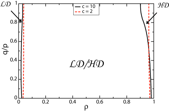
Figure 12: The $(q/p,\rho)$-phase diagram for PASEP through irregular networks. We plot the boundaries between different regimes for single graph instances with $c=10$, $|V|=200$ and $c=2,|V|=607$ at $L=\infty$. The $\mathcal{LD}$/ $\mathcal{HD}$ regime remains present in the limit $q/p\rightarrow 1$.

4.5 Discussion

We conclude that the stationary state of bi-directional transport on networks has similar characteristics to that of uni-directional transport. Indeed, PASEP on networks leads to stationary regimes which have their direct equivalent in TASEP: regular networks feature $\mathcal{LD}$, $\mathcal{LD-HD}$ and $\mathcal{HD}$ regimes, while irregular networks are dominated by the $\mathcal{LD/HD}$ regime. From these results it follows that the degree of asymmetry does not change the qualitative picture for the emergence of density heterogeneities in cytoskeletal motor protein transport.

Another interesting point is that the network topology affects how the stationary state reaches the passive equilibrium case of $q\approx p$. In regular networks density heterogeneities disappear gradually: the heterogeneous $\mathcal{LD-HD}$ segment regime reduces gradually in size to eventually disappear at $q=p$, see figure 10-(a). In the symmetric limit particles therefore spread completely homogeneously for all particle densities. In irregular networks the phenomenology is very different: density heterogeneities do not disappear gradually when reaching the symmetric limit, see figure 12. The heterogeneous $\mathcal{LD/HD}$ network regime remains present for all values $q<p$ when $L$ is large enough, leading to strong density heterogeneities on the network. This situation is visualized in figure 13.

The simulation results also show that, in irregular networks, finite size effects play a role close to the symmetric case ($p\approx q$). To identify the crossover from an active to a passive process on irregular networks we have studied the distribution of particle densities as a function of the segment length $L$ at values $q\approx p$. Then particles are seen to be distributed homogeneously along the network for short segments, whereas they are distributed heterogeneously over the network for longer segments. This can be quantified with the distribution of segment densities (figure 11): this distribution is unimodal for small $L$ and becomes trimodal at large $L$. Interestingly this implies that for a close to symmetric process ($q\approx p$) on irregular networks there is a crossover from a passive to an active process in terms of the segment length $L$.

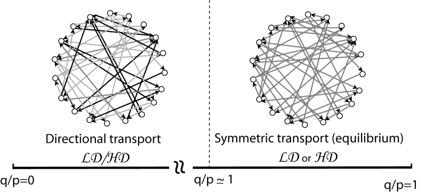
Figure 13: Visualization of the stationary state of PASEP through irregular networks as a function of the fraction between the hopping rates $p/q$. When $p/q=0$ we find a stationary state in the $\mathcal{LD/HD}$ regime corresponding to TASEP through irregular networks, while for $p/q=1$ we recover the homogeneous equilibrium distribution. The crossover from a heterogeneous to a homogeneous distribution of particles happens at $p/q\approx 1$, and at $p/q=1$ for $L\rightarrow\infty$.

5 Particles with finite processivity

In the previous sections we have considered transport through closed networks. However, cytoskeletal transport poses an additional challenge, since motors only have a finite processivity: they can stochastically attach and detach at any point in the network, thereby alternating stretches of directed motion on the network with diffusive motion in the cytoplasm, see figure 1.

Here we model this behaviour based on the TASEP-LK, which we generalize to transport along a network [53]. Particle attachment and detachment is governed by the rates $\omega_{A}$ and $\omega_{D}$, respectively. The particle reservoir is considered to be infinitely large, and diffusion is assumed to guarantee a uniform distribution in the bulk. In this process the total particle density along the network is seen to be set directly by the Langmuir exchange with the reservoir, through the ratio between the attachment and detachment rates. In contrast, the way in which particles are distributed along the network requires understanding of the intricate interplay between the effect of infinite diffusion (in the reservoir) and active transport (along the network). This model is summarized graphically in Fig. 14.

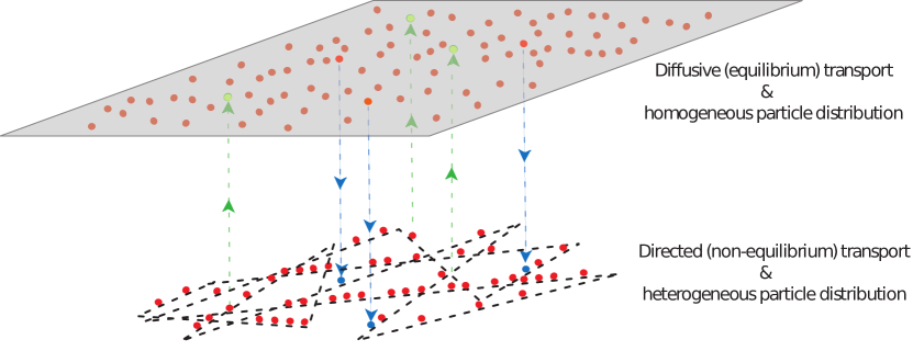
Figure 14: Illustration of the totally asymmetric exclusion process with Langmuir kinetics (TASEP-LK). Particles moving actively along a network are exchanged with a bulk reservoir, in which they diffuse. This leads to a competition between an active non-equilibrium transport process on one hand, which entails a heterogeneous distribution of particles along the network, and a passive diffusion transport process, which aims at a homogeneous equilibrium distribution of particles. Three parameters are relevant for this interplay: the topology of the network, the total particle density $\rho$ (equivalent to the parameter $K$), and the relative exchange rate $\Omega=\omega L/p$ (the latter taking in account the total exchange rate between reservoir and network $\omega$, the segment length $L$ and the particle hopping rate along the network $p$).

Indeed, the passive diffusion process in the reservoir tends to spread particles out homogeneously, and therefore also has a homogenizing effect on the network. Active transport on the other hand has been seen above to provoke density heterogeneities (see sections 3 and 4). Since the bulk diffusion in the reservoir is assumed to be infinitely fast, the active dynamics may be expected intuitively to impose heterogeneities along the network if their motion is sufficiently processive. We will now analyze in detail this interplay between passive diffusion and active transport and how it regulates the distribution of particles on the network. These complement the results presented briefly in [53].

We first revisit the macroscopic behaviour of TASEP-LK on a single open segment [58, 59]. In a second subsection we define TASEP-LK on a network, determine the corresponding mean-field equations and present the effective rate diagrams. We then present a way to establish analytical solutions to the mean-field equations if the particle exchange with the reservoir is sufficiently strong, due to a decoupling of the continuity equations. In the subsequent sections we elaborate on the stationary state of regular and irregular networks, including the infinitely connected limit. We end by discussing the results of this section and put them into the context of biophysical experiments.

5.1 TASEP-LK on a single open segment

TASEP-LK is similar to TASEP in that particles hop uni-directionally along a one-dimensional segment at rate $p$ and are subject to exclusion interactions. In addition, particles attach and detach along the segment according to a Langmuir process [88]. In the single segment model, we are thus dealing with three reservoirs: the two reservoirs at the entrance and the exit of the segment (rates $\alpha$ and $\beta$) are now complemented by a bulk reservoir, which allows for binding/unbinding of particles on any site along the segment with rates $\omega_{A}$ and $\omega_{D}$, respectively. We have illustrated this process in figure 4-(d).

New behaviour emerges in TASEP-LK if there is a competition between the directed transport and the Langmuir kinetics (LK), which is the case in the so-called ’scaling’ regime [59], $\omega_{A}=p\>\Omega_{A}/L$, $\omega_{D}=p\>\Omega_{D}/L$ (note that $\Omega_{A}$ and $\Omega_{D}$ are dimensionless). In this scaling regime the dynamics of the bulk is in competition with the dynamics at the boundaries, which leads to an interesting $(\alpha,\beta)$-phase diagram [58, 59], represented in the appendix, figure 25. Indeed, the resulting density profiles in the segment interpolate between those of TASEP and the homogeneous profiles of a Langmuir process: on one hand the TASEP density profiles are recovered for small attachment/detachment rates ($\Omega_{A},\Omega_{D}\rightarrow 0$), and on the other hand the homogeneous Langmuir profile with an equilibrium density

$$\rho_{l}=\frac{\Omega_{A}}{\Omega_{D}+\Omega_{A}}$$ (27)

is observed for large attachment/detachment rates ($\Omega_{A},\Omega_{D}\rightarrow\infty$). On a single segment these current and density profiles have been determined from mean-field arguments and are well corroborated by numerical simulations [58, 59]. They are conveniently expressed as a function of the rescaled position variable along the segment, $x=i/L\in[0,1]$, with $i=1..L$. Since TASEP-LK is an exclusion process we have a parabolic expression in the current-density relationship:

$$J^{\rm LK}\left[x;\alpha,\beta,\Omega_{A},\Omega_{D}\right]=p\>\rho^{\rm LK}\left[x;\alpha,\beta,\Omega_{A},\Omega_{D}\right]\left(1-\rho^{\rm LK}\left[x;\alpha,\beta,\Omega_{A},\Omega_{D}\right]\right).$$ (28)

The full expressions for $J^{\rm LK}$ and $\rho^{\rm LK}$ are discussed in A. Note also that, due to particle binding/unbinding, the current is no longer constant along the segment. Consequently we must account for the fact that the current entering a segment will generally differ from the current leaving the same segment.

We will require the phase diagrams of TASEP-LK on a single segment for our analysis of the stationary state on a network, using effective rate diagrams. We therefore discuss them briefly here; a more elaborate discussion is presented in A and in figure A1. It is useful to introduce the parameters $K=\Omega_{A}/\Omega_{D}$ and $\Omega=(\Omega_{A}+\Omega_{D})/2$. The quantity $\Omega$ characterizes the overall exchange between the bulk reservoir and the segment, whereas the ratio in $K$ directly determines the Langmuir density imposed by the exchange with the bulk reservoir (equation (27)). The phase diagrams for TASEP-LK display several phases: ’pure’ LD, HD, and MC (also referred to as the M phase in some previous works [59]), as well as the combined phases LD-HD, LD-MC and MC-HD. Recall also that LD, HD and MC phases are in fact the appropriate generalizations of the corresponding phases in TASEP, with the difference that their density profiles are no longer constant throughout the segment. The density variation along the segment is continuous in all pure phases, but a discontinuous shock arises for the combined phases. For example, in the LD-HD phase the shock corresponds to a domain wall at some position $x_{w}$. When $\Omega\rightarrow 0$ this LD-HD phase reduces to the $\alpha=\beta<p/2$ coexistence line and we recover the TASEP phase diagram as expected. For $\Omega\rightarrow\infty$ the LD-HD phase becomes more prominent and is eventually present for all $\alpha/p<(K+1)^{-1}$ with $\beta/p<1/2$ when $K>1$. At high $\Omega$ the LD phase then disappears altogether from the phase diagram. More precisely this happens at the threshold $\Omega_{c}$ given by equation (71) in Appendix A. Similarly, the HD phase disappears from the phase diagram for $K<1$ at a value $\Omega_{c}$.

An important notion in the study of TASEP-LK on networks is the distinction between those phases which couple boundaries and those which uncouple them. This concept is illustrated in figure 15. In the LD phase (or the HD phase), changing the entrance rate $\alpha$ (or exit rate $\beta$) modifies the bulk density and current throughout the whole segment, right through to the end of the segment. In this sense the boundaries can be considered to be coupled, as is illustrated on the left of figure 15. In the LD-HD phase on the other hand, changing the rate $\alpha$ at the left boundary only modifies the current and density over a finite portion of the segment, but it does not affect the density at the right boundary of the segment. In that sense the boundaries are uncoupled, see the right of figure 15. Note that the discontinuity in the density profile at $x=x_{w}$ uncouples the LD region at the entrance from the HD region at the exit of the segment. Hence boundaries are uncoupled in the LD-HD phase due to the presence of a shock. In the phases involving MC the boundaries are also decoupled.

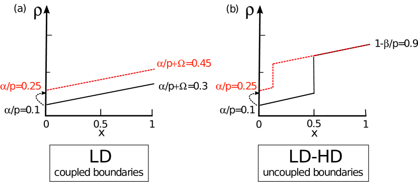
Figure 15: Density profiles $\rho_{s}(x)$ as a function of the rescaled position $x\in[0,1]$ in the segment are presented for TASEP-LK. A boundary dependent phase (left) is compared with a boundary independent phase (right). Left (a): In the LD phase the density at the exit $x=1$ changes when the entrance rate is modified: both boundaries are coupled. Right (b): In the LD-HD coexistence phase, the density at the exit $x=1$ does not change with the entrance rate: hence both boundaries are decoupled.

5.2 Effective rate diagrams describing TASEP-LK on networks

As a first observation we point out that for TASEP-LK, although density heterogeneities arise throughout the network, the overall density $\rho$ is directly set to the Langmuir density ($\rho=\rho_{\ell}=K/(K+1)$). We will show that it is the exchange parameter $\Omega$ which regulates the distribution of particles on the network.

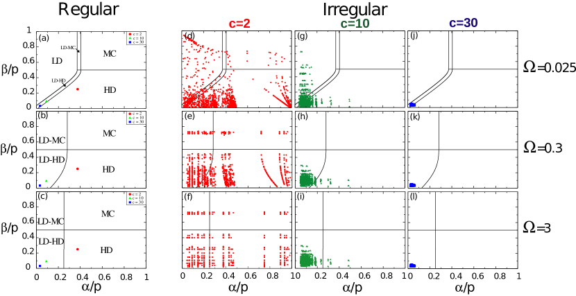
Figure 16: Effective rate diagrams for TASEP-LK through regular graphs (left, (a)-(c)) and irregular graphs (right, (d)-(l)), both filled to a total density of $\rho=3/4$, are presented for the given values of $\Omega$ and $c$. We have used the same graph instances as in figure 5. On regular graphs the effective rates are equal for all segments, such that only one marker is plotted.

The TASEP-LK model on a network can be studied using the general mean-field method presented in subsection 2.3. The currents $J^{-}\left[\alpha_{s},\beta_{s}\right]$ and $J^{+}\left[\alpha_{s},\beta_{s}\right]$ entering and leaving a segment in equation (2) follow, respectively, from the mean-field current profiles $J^{\rm LK}\left[x=0;\alpha_{s},\beta_{s},\Omega_{A},\Omega_{D}\right]$ and $J^{\rm LK}\left[x=1;\alpha_{s},\beta_{s},\Omega_{A},\Omega_{D}\right]$ along a single segment (see equation (28) and the expressions for the density in the A). Since particles can attach/detach along the segment we have now $J^{+}\neq J^{-}$ in the continuity equation (2). We establish the effective rates as $\alpha^{\rm eff}_{(v,v^{\prime})}=p\>\rho_{v}/c^{\rm out}_{v}$ and $\beta^{\rm eff}=p\>(1-\rho_{v})$, corresponding to a uniform microscopic hopping rate at the junctions. Note that these are the same effective rates as presented for TASEP in equations (11): this reflects the fact that attachment/detachment at the junction sites themselves is negligible in the scaling regime. The resulting mean-field equations (2) for the average junction densities of TASEP-LK are then given by

$$\frac{\partial}{\partial t}\rho_{v} = \sum_{v^{\prime}\rightarrow v}\>J^{\rm LK}\left[x{=}1;\frac{\rho_{v^{\prime}}}{c^{\rm out}_{v^{\prime}}},1{-}\rho_{v},\Omega_{A},\Omega_{D}\right]-\sum_{v^{\prime}\leftarrow v}J^{\rm LK}\left[x{=}0;\frac{\rho_{v}}{c^{\rm out}_{v}},1{-}\rho_{v^{\prime}},\Omega_{A},\Omega_{D}\right].$$ (29)

We have solved the mean field equations (29) and mapped the effective rates of each of the individual segments of the network onto the corresponding $(\alpha,\beta)$-phase diagrams of a single segment. These results, presented in figure 16, characterize the stationary state of TASEP-LK through networks.

Several interesting features emerge from these diagrams. The stationary state of TASEP-LK shares certain characteristics with TASEP and PASEP. For regular graphs all effective rates have the same value and coincide in one point in the effective rate diagram. Irregular graphs on the other hand lead to a scattered plot of all effective rates, and they cluster around the origin at high connectivities (as can be understood in terms of bottleneck formation). However, the LD-HD coexistence increasingly widens with increasing exchange parameter $\Omega$, which has a direct impact onto the phenomenology of density heterogeneities. Moreover, we now see that the scatter plots which appear random at low exchange parameters $\Omega$ reveal a certain regularity at high values of $\Omega$. In this range effective rates become independent of $\Omega$, as well as being independent of global topological features of the network (i.e. they only depend on the local junction degrees). This feature can be explained using the notion of coupled and uncoupled boundaries introduced at the end of the previous subsection.

5.3 Uncoupling of boundaries at high $\Omega$: simplified mean-field equations

At weak exchange (small $\Omega$), close to the TASEP limit ($\Omega=0$), the continuity equations (29) in the junction densities are intrinsically coupled. Indeed, a large fraction of the segments will be in the LD or HD phase and couple their boundaries. Finding a solution then typically requires a numerical procedure. However, when increasing $\Omega$ more and more segments switch into a LD-HD phase (see figure 16), reducing the coupling. For sufficiently high $\Omega$ the continuity equations (29) uncouple, providing a route to an exact solution to the mean-field equations. In particular, we can present an exact solution of the continuity equations for any graph, based on the single segment phase diagram for $\Omega\rightarrow\infty$. It will turn out that this solution remains accurate down to rather small values of $\Omega$, which we rationalize in terms of the effective rate diagrams.

Before considering the solution in the $\Omega\rightarrow\infty$ limit, which is valid for any graph topology, let us first consider the simpler case for which all segments in the network are in the LD-HD phase. From the effective rate diagrams figure 16 we see that this is the case for regular graphs and for irregular graphs at high connectivities. When all segments are in the LD-HD phase, modifying the density at a certain junction will not change the density of particles at other junctions in the network: the domain walls in each of the segments block the propagation of density perturbations from the adjacent junction. The continuity equations (29) then simplify into

$$\frac{\partial}{\partial t}\rho_{v} = c^{\rm in}_{v}J^{-}_{v}-c^{\rm out}_{v}J^{+}_{v}$$ (30)

$$= c^{\rm in}_{v}\rho_{v}(1-\rho_{v})-\rho_{v}\left(1-\frac{\rho_{v}}{c^{\rm out}_{v}}\right).$$ (31)

We see that the currents at the junctions $J^{\pm}_{v}$ only depend on the local junction density $\rho_{v}$, such that the continuity equations (29) are completely decoupled. We obtain the solution

$$\rho_{v} = \frac{c^{\rm in}_{v}-1}{c^{\rm in}_{v}-\left(c^{\rm out}_{v}\right)^{-1}}.$$ (32)

Equations (32) are valid for networks at high enough connectivities and exchange rates $\Omega$, and this is due to two combined effects: increasing the connectivity effective rates cluster around the origin, whereas increasing $\Omega$ enlarges the LD-HD region in the phase diagram (see figure 16).

We consider now the limiting case $\Omega\rightarrow\infty$, for which we can solve the mean-field equations (29) analytically using uncoupling of boundaries. Depending on the overall particle density $\rho=K/(K+1)$ we find the solutions:

• $\rho>1/2$:

  $$\rho_{v} = \left\{\begin{array}[]{cccc}c^{\rm out}_{v}\left(\frac{c^{\rm in}_{v}-1}{c^{\rm out}_{v}c^{\rm in}_{v}-1}\right)&&&\frac{\rho_{v}}{c^{\rm out}_{v}}\leq 1-\rho\ {\rm and}\ c^{\rm in}_{v}\neq 1\\ \frac{c^{\rm out}_{v}}{2}\left(1-\sqrt{1-\left(c^{\rm out}_{v}\right)^{-1}}\right)&{\rm for}&&\frac{\rho_{v}}{c^{\rm out}_{v}}\leq 1-\rho\ {\rm and}\ c^{\rm in}_{v}=1\\ \frac{1}{2}\left(1+\sqrt{1-4\>\frac{c^{\rm out}_{v}}{c^{\rm in}_{v}}\rho(1-\rho)}\right)&&&\frac{\rho_{v}}{c^{\rm out}_{v}}\geq 1-\rho\ {\rm and}\ \rho_{v}\geq 1/2\end{array}\right.$$ (36)

• $\rho=1/2$:

  $$\rho_{v} = \left\{\begin{array}[]{cccc}c^{\rm out}_{v}\left(\frac{c^{\rm in}_{v}-1}{c^{\rm out}_{v}c^{\rm in}_{v}-1}\right)&&&c^{\rm in}_{v}\neq 1,\>c^{\rm out}_{v}\neq 1\\ \frac{c^{\rm out}_{v}}{2}\left(1-\sqrt{1-\left(c^{\rm out}_{v}\right)^{-1}}\right)&&{\rm for}&c^{\rm in}_{v}=1\\ \frac{1}{2}\left(1+\sqrt{1-\left(c^{\rm in}_{v}\right)^{-1}}\right)&&&c^{\rm out}_{v}=1\\ \end{array}\right.$$ (40)

• $\rho<1/2$:

  $$\rho_{v} = \left\{\begin{array}[]{cccc}c^{\rm out}_{v}\left(\frac{c^{\rm in}_{v}-1}{c^{\rm out}_{v}c^{\rm in}_{v}-1}\right)&&&\rho_{v}\geq 1-\rho\ {\rm and}\ c^{\rm out}_{v}\neq 1\\ \frac{1}{2}\left(1+\sqrt{1-\left(c^{\rm in}_{v}\right)^{-1}}\right)&{\rm for}&&\rho_{v}\geq 1-\rho\ {\rm and}\ c^{\rm out}_{v}=1\\ \frac{c^{\rm out}_{v}}{2}\left(1-\sqrt{1-4\>\frac{c^{\rm in}_{v}}{c^{\rm out}_{v}}\rho(1-\rho)}\right)&&&\rho_{v}<1-\rho\end{array}\right.$$ (44)

These solutions in the junction densities $\rho_{v}$ are valid for $c^{\rm in}_{v}\neq 0$ and $c^{\rm out}_{v}\neq 0$. When $c^{\rm in}_{v}=0$ the density will be trivially equal to $\rho_{v}=0$, whereas for $c^{\rm out}_{v}=0$ the junction density takes the value $\rho_{v}=1$.

The way to derive the above equation goes as follow: we consider the phase diagram of TASEP-LK in the limit $\Omega\rightarrow\infty$, see bottom of figure 25. In this limit one notices that boundaries decouple, i.e. $\alpha^{\rm eff}_{v\rightarrow v^{\prime}}$ is only a function of $\rho_{v}/c^{\rm out}_{v}$ (and not of $\rho_{v^{\prime}}$) and $\beta^{\rm eff}_{v\rightarrow v^{\prime}}$ is only a function of $\rho_{v}^{\prime}$ (and not of $\rho_{v}$). In the end, after considering the different phases at $\Omega\rightarrow\infty$, decoupling allows us to solve exactly the full mean-field equations (29) leading to equations (40). Note that, when combined with the expressions for the segment and density profiles $J^{\rm LK}$ and $\rho^{\rm LK}$ in A, equations (40) give us analytical expressions for the stationary density and segment profiles of all the segments in the network.

The simplified mean-field equations (40) provide an explanation as to why the effective rate diagrams for irregular graphs (figure 16), which contain randomly scattered effective rates at low values of $\Omega$, become more ordered at high values of $\Omega$. Indeed, the decoupling leads to junction densities which only depend on the local degrees $c^{\rm in}_{v}$ and $c^{\rm out}_{v}$, as well as the stationary density $\rho$. The effective rate plots at strong exchange $\Omega$ are thus independent of $\Omega$ and of the global random topology of the network.

Equations (40) can also be seen as an approximation to the full mean-field equations (29) at finite $\Omega$. In figure 17 we compare the current profiles of the full equations (29), both with the simplified version equation (40) and with simulations. Results are presented for irregular graphs of given mean connectivity $c$ and with a given stationary density $\rho$. Just as expected, simulation results are in very good agreement with those obtained by numerically solving the full mean-field equations. But remarkably we find that the simplified mean-field result gives already a very accurate approximation, and this is true down to rather weak exchange parameters ($\Omega\gtrsim 0.5$). This can be understood from the shape of the single segment phase diagram which remains similar to the one for $\Omega\rightarrow\infty$.

Moreover, the simplified equations (40) are exact in special circumstances. This is the case at half-filling ($\rho=1/2$), for any exchange parameter $\Omega\geq 0.5$, since then the decoupling is complete (see C). It also applies asymptotically at high connectivities $c$: as one can see from figures 16, the effective rates indeed cluster around the origin in the LD-HD phase in this limit, which again leads to full decoupling. In contrast, the decoupled description by equations (40) becomes less accurate for densities $\rho\rightarrow 0$ or $\rho\rightarrow 1$, since then the zone corresponding to the decoupled LD-HD phase becomes very small in the effective rate diagrams.

To summarize, in this subsection we have shown that the mean-field description of TASEP-LK simplifies when increasing the exchange rate with the reservoir $\Omega$. We have derived analytical expressions for the stationary density and current profiles throughout the network which are very accurate at sufficiently high exchange parameters $\Omega$ and mean connectivities $c$, as well as for stationary densities $\rho$ close to half filling.

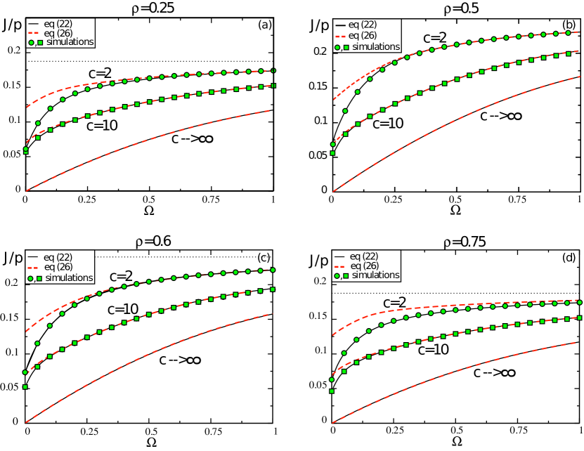
Figure 17: The average current $J$ for TASEP-LK through irregular networks, as a function of the exchange rate $\Omega$ for given particle filling $\rho$ and mean connectivity $c$. Full mean-field results of equations (29) (solid lines) are compared with simulation data (markers) and the solution to the simplified mean field equations (40) (rad dashed lines). Mean field results are for single graph instances of mean connectivity $c=2$ and $|V|=607$ junctions or $c=10$ and $|V|=200$. Simulations are run on the same graphs with segments of length $L=400$. Further represented are: the upper bound to the average current given by the Langmuir expression $\rho(1-\rho)$ (dotted line) and its lower bound, given by graphs with mean connectivity $c\rightarrow\infty$.

5.4 Networks of infinite connectivity

We now discuss the stationary state of networks for which the vertex degree of each junction is very high. For $\Omega>0$ all segments fall into the LD-HD phase since the effective rates cluster around the origin. Thus, the network is in the $\mathcal{LD-HD}$ regime and the simplified solution (40) based on the decoupling of segments is exact (within the mean field framework). In this limit the stationary current and density profiles can be computed analytically by setting $\rho_{v}=1$, see B. In particular, for half filling $\rho=1/2$ we present a simple expression in C. Knowing the exact expression for the current in the infinitely connected limit is interesting for two reasons.

First, as one can see from figure 17, the current reaches in this limit ($c\rightarrow\infty$) the minimal value accessible for the given values of $\Omega$ and $\rho$. This is in fact intuitive, since all junctions become fully blocked and suppress all flow through the junctions. But for TASEP-LK these junction bottlenecks do not block the dynamics in the segments completely, as long as there is a non-zero exchange rate $\Omega>0$: figure 17 shows that, even for small values of $\Omega$, the current does not reduce to zero when $c\rightarrow\infty$. This indicates that even a weak exchange with a reservoir is sufficient for particles to circumvent bottlenecks and maintain a significant flow through the network.

A second reason which makes the strong connectivity limit special is that all networks behave identically, as long as $\Omega>0$. Hence, in this limit the stationary state of all networks is the same and we recover a universal, topology independent stationary state. The reason for this universality is twofold. First, for $c\rightarrow\infty$ the LD-HD phase dominates, such that perturbations remain local and do not propagate throughout the network due to the continuity equations (29). Second, all junctions become infinite bottlenecks, such that $(\alpha,\beta)\rightarrow\mathcal{O}(c^{-1},c^{-1})$. As a consequence the currents and densities in the segments are rather insensitive to local degree fluctuations.

5.5 TASEP on LK through regular networks

Regular networks constitute another solvable case for TASEP-LK. Just as for TASEP and PASEP, the stationary state of TASEP-LK on regular networks is given by a unique junction occupancy $\rho_{v}$ for all junctions. We find the following solution to the mean field equations (29):

$$\rho_{v}\left[\Omega,\rho\right] = \left\{\begin{array}[]{lllll}c\rho&&\rho<1/(c+1)&&(\mathcal{LD})\\ c/(c+1)&&1/(c+1)<\rho<c/(c+1)&&(\mathcal{LD-HD})\\ \rho&&\rho>c/(c+1)&&(\mathcal{HD})\end{array}\right.$$ (48)

Remarkably, this solution is identical to the one for TASEP [52]. This can be seen as follows. Recall that $c^{\rm out}_{v}=c^{\rm in}_{v}=c$ at all junctions $v$ for regular graphs, such that all junctions (and therefore all segments) are equivalent. Current conservation at the junctions, equation (29), then implies that we must have $J_{+}=J_{-}$ for all segments. This points to either a solution for which the segments have a homogeneous density (and are thus in the LD or HD phase) or to a solution for which the segments have a heterogeneous density with $\alpha^{\rm eff}=\beta^{\rm eff}$ (and are in the LD-HD coexistence phase). The presence of a homogeneous density profile in the segments may appear counter-intuitive, since the exchange process with the bulk typically leads to non-homogeneous density profiles (unless $\Omega\rightarrow\infty)$. But this proves to be correct from the solution for a single segment: equation (70), in A, shows that a homogeneous solution is possible, provided $\beta^{\rm eff}=(1-\rho_{\ell})=(1-\rho)$ at HD and $\alpha^{\rm eff}=\rho_{\ell}=\rho$ at LD. Using that $(\alpha^{\rm eff},\beta^{\rm eff})=(\rho_{v}/c,1-\rho_{v})$ leads immediatly to the solution equation (48). In essence, these arguments show that the homogeneous density profile (48) is the correct solution for a regular network, even for a finite exchange parameter $\Omega$. In the intermediate case, when the segments are in the coexistence phase, the junction densities and effective rates follow immediately from the simplified mean field equation (40), and are given by $\rho_{v}=c/(c+1)$. We thus see that, just as for TASEP, we are dealing with a LD phase $\alpha^{\rm eff}<\beta^{\rm eff}$, a HD phase when $\beta^{\rm eff}<\alpha^{\rm eff}$ and a coexistence phase at $\beta^{\rm eff}=\alpha^{\rm eff}$.

From the solution (48) for the junction densities we can deduce the phase diagram in figure 18-(a) for TASEP-LK through regular graphs. Figure 18-(a) shows that the same behaviour arises as in TASEP, i.e. with increasing density we successively observe a $\mathcal{LD}$ regime, a heterogeneous $\mathcal{LD-HD}$ segment regime, and finally a $\mathcal{HD}$ regime. The density zone for the $\mathcal{LD-HD}$ segment regime is identified as $1/(c+1)<\rho<c/(c+1)$, and remarkably is altogether independent of the exchange parameter $\Omega$. This observation implies that the $\mathcal{LD-HD}$ does not disappear when approaching the equilibrium process ($\Omega\rightarrow\infty$). Note that this behaviour is very different from PASEP, where the symmetric limit ($p/q\rightarrow 1$) makes the segment regime disappear (compare figures 18-(a) and 10-(a)).

This equilibrium limit $\Omega\rightarrow\infty$ can be understood as follows. The inhomogeneous density profile with a domain wall, located at some position $x_{w}$, persists for $\Omega\rightarrow\infty$. In fact, as $\Omega$ increases the position $x_{w}$ will gradually move to one of the segment ends ($x_{w}\rightarrow 0$ for $\rho>1/2$ or $x_{w}\rightarrow 1$ for $\rho<1/2$, half-filling $\rho=1/2$ is special, see C). This constitutes a way of asymptotically restoring homogeneity within single segments, although the $\mathcal{LD-HD}$ regime is maintained for the network. This analysis is further corraborated by the current-density relation $J(\rho)$, which indirectly provides a measure for the degree of heterogeneity within the segments: a parabolic profile $J=\rho(1-\rho)$ corresponds to a homogeneous density profile, whereas deviations from the parabola indicate a hinderance due to heterogeneities. From figure 18-(b) we see that for $\Omega\rightarrow\infty$ the current-density profile gradually reaches the parabolic Langmuir profile $J=\rho(1-\rho)$, thus showing that the homogeneous equilibrium profile is eventually attained.

An analytical expression for the current density profile follows by using the formulas in A and the solution given by equations (48). However, only in the case of half-filling is it simple to establish these expressions (see C).

In summary, TASEP-LK through regular networks leads to the same regimes of heterogeneities as TASEP through regular networks. The size of the zone corresponding to the heterogeneous $\mathcal{LD-HD}$ regime is not affected by the coupling with the reservoir. The equilibrium process is attained as the LD-HD domain walls in all segments shift towards the junction sites.

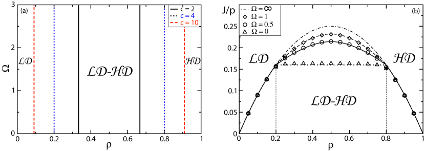
Figure 18: TASEP-LK through regular graphs. Left (a): The lines separating the $\mathcal{LD}$ and $\mathcal{LD-HD}$ regimes, as well as the $\mathcal{LD-HD}$ and $\mathcal{HD}$ regimes are presented as a function of the total density $\rho$ and the exchange parameter $\Omega$ for regular graphs of given degre $c$. Right (b): Average current-density profile for regular graphs of degree $c=4$. Mean-field results (solid lines) are compared with simulation data (markers) on graphs of $|V|=80$ junctions and segments of length $L=400$, for different values of the exchange rates $\Omega$. For $\Omega\rightarrow\infty$ the transport process becomes passive. We obtain a parabolic profile in this limit, indicating a homogeneous density distribution at all scales.

5.6 TASEP-LK through irregular networks

We now determine the stationary state of TASEP-LK through irregular networks. It can be understood using effective rate diagrams (figures 16) and the classification in three different regimes for the particle distribution, as developed in section 3 (see figure 8).

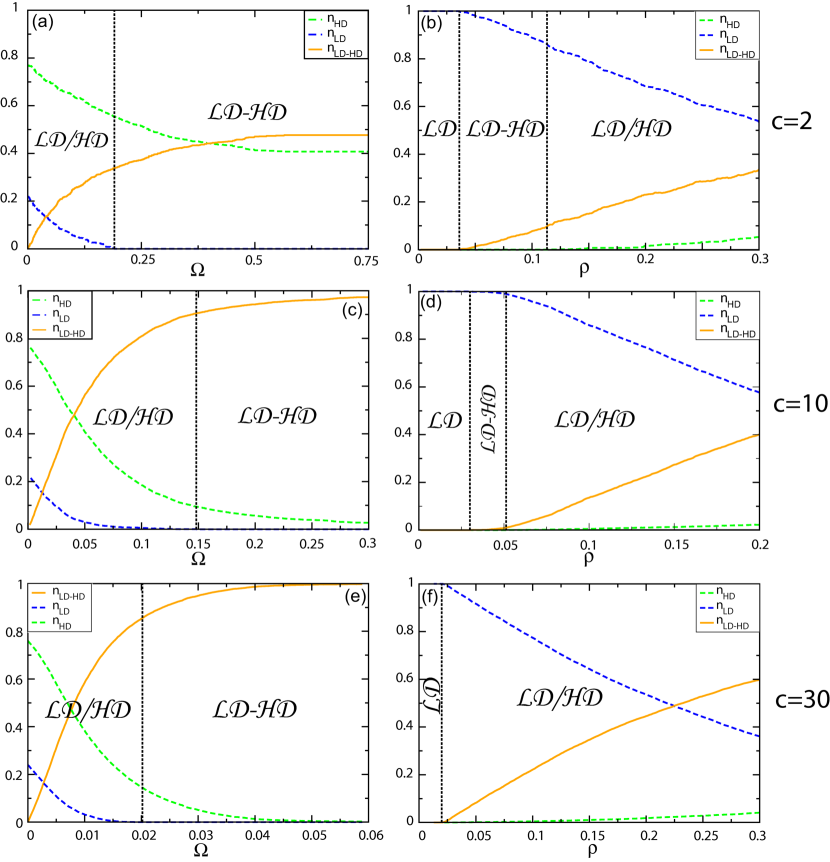
Figure 19: The fraction of segments in the LD phase, the HD phase and the LD-HD phase as a function of $\Omega$ and $\rho$ for TASEP-LK for single instances of irregular graphs at given mean connectivity $c$ (the fractions for M, M-HD and LD-M are small and not represented). We have $\rho=0.75$, $c=2$ (a), $\Omega=0.15$, $c=2$ (b), $\rho=0.75$, $c=10$ (c), $\Omega=0.05$, $c=10$ (d), $\rho=0.75$, $c=30$ (e), $\Omega=0.01$, $c=30$ (f). The graphs used have $|V|=607$ junctions ($c=2$), $|V|=500$ ($c=10$) and $|V|=500$ ($c=30$). The transitions between the stationary regimes of density heterogeneities are indicated: $\mathcal{LD}$ homogeneous, $\mathcal{HD}$ homogeneous, $\mathcal{LD-HD}$ heterogeneous and $\mathcal{LD/HD}$ heterogeneous.

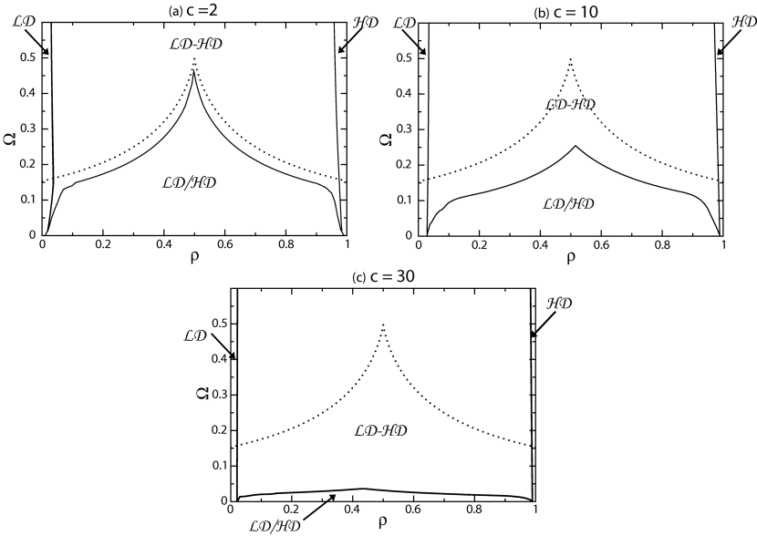
Figure 20: The $(\Omega,\rho)$-diagram for TASEP-LK through irregular graphs. The transitions (solid lines) between the different regimes of the stationary state on the network are shown for the same graph instances as in figure 19. The dotted line shows the upper bound to the transition between the heterogeneous network $(\mathcal{LD/HD})$ and segment $(\mathcal{LD-HD})$ regimes (as given by equation 49).

To identify the regime for the stationary state (i.e. $\mathcal{LD}$, $\mathcal{HD}$, $\mathcal{LD-HD}$ and $\mathcal{LD/HD}$) we need to determine the fraction of segments in the network which occupy the different phases (i.e. LD, HD, LD-HD) in the effective rate diagrams, figure 16. We denote these fractions by $n_{\rm LD}$, $n_{\rm HD}$, $n_{\rm LD-HD}$; the M, LD-M and M-HD phases play a minor role and will not be considered. In figure 19 these fractions are shown as a function of $\Omega$ and $\rho$. Using the definitions of the different network regimes given in figure 8 we can establish the boundaries of the corresponding zones in the $(\rho,\Omega)$ plane. We have indicated the resulting phase diagrams in figure 20 for irregular networks.

We note several interesting characteristics of the stationary state on irregular networks. To do so let us focus on the case $\rho>1/2$ (similar arguments apply for $\rho<1/2$). At low exchange parameters $\Omega$ the network is in the $\mathcal{LD/HD}$ regime: a finite fraction of segments occupy the LD and HD phases. The strong heterogeneities in the particle densities are reflected in the bimodal distribution of segment densities, as shown in figure 21. For vanishing exchange ($\Omega\rightarrow 0$), we recover the results for TASEP with infinite processivity presented in section 3. However, when we decrease the processivity (i.e. for an increasing $\Omega$), the LD phase in the effective rate plane shrinks in favour of the LD-HD phase, see figure 16. Eventually the fraction of segments in LD reduces to zero, $n_{\rm LD}=0$, and the network enters the $\mathcal{LD-HD}$ regime. In this segment regime the density heterogeneities are mainly attributable to the LD-HD domain walls which separate a LD and a HD part on the same segment. The average density between single segments however does not vary much throughout the network in this phase. Indeed, the distribution of segment densities is unimodal in the $\mathcal{LD-HD}$ regime, see figure 21. We also note that at very high densities ($\rho\approx 1$), the stationary state is in a homogeneous regime where $n_{\rm LD}=n_{\rm LD-HD}=0$, and thus all segments are in the HD phase ($n_{\rm HD}=1$). In this regime, even the heterogeneities within single segments have disappeared.

The boundaries between the different regimes are easily understood from the effective rate diagrams figure 16. Let us for instance consider the transition from the $\mathcal{LD/HD}$ to the $\mathcal{LD-HD}$ regime. With an increasing exchange parameter $\Omega$ the size of the LD phase decreases in the single-segment $(\alpha,\beta)$-phase diagram. At some point the LD phase is so small that no segments occupy this phase anymore: this marks the boundary between the network and the segment regime. This happens at the critical value $\Omega_{c}(\rho)$, at which the LD phase (or HD phase for $\rho<1/2$) in the $(\alpha,\beta)$-phase diagram (of a single segment) has completely disappeared. This critical value is given by (see equation (71)):

$$\Omega_{c}=\frac{1}{2}+\left|\rho-\frac{1}{2}\right|\ln\left[\frac{\left|\rho-1/2\right|}{1/2+\left|\rho-1/2\right|}\right].$$ (49)

This expression (49) is illustrated in figure 20 through the dotted line. Also the transitions from the $\mathcal{LD-HD}$ segment regime to the homogeneous $\mathcal{LD}$ regime can be understood intuitively from the effective rate diagram: when decreasing $\rho$ towards zero, the LD-HD phase becomes gradually smaller and retracts to the axis $\beta=0$, while the effective rates move towards $\beta=1$. A similar argument applies to the transition from $\mathcal{LD-HD}$ to $\mathcal{HD}$, for $\rho\rightarrow 1$.

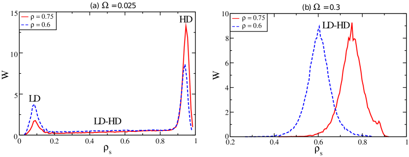
Figure 21: Distribution of segment densities $W(\rho_{s})$ of TASEP-LK on an irregular graph with mean connectivity $c=10$ at given total densities $\rho$ and exchange rates $\Omega$. Mean-field results on a single graph instance of size $|V|\approx 10^{4}$ are presented. (a): for low values of $\Omega$ the distribution is bimodal, with the two peaks corresponding to segments in the LD and the HD phases. The broad intermediate ”band” corresponds to segments in the LD-HD phase. The stationary state of the network is in the heterogeneous network regime $(\mathcal{LD/HD})$. (b):at the value $\Omega=0.3$ segments are in the LD-HD phase and the distribution is unimodal. The network is in the heterogeneous segment regime $(\mathcal{LD-HD})$.

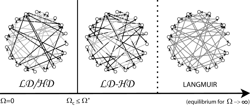
Figure 22: Visualization of the stationary state of TASEP-LK on irregular networks when varying the total exchange $\Omega$ and keeping the total density $\rho$ fixed. The way particles are distributed changes qualitatively when the exchange parameter $\Omega$ is varied: the stationary state first shifts from a $\mathcal{LD/HD}$ regime to a $\mathcal{LD-HD}$ regime, indicating that the density heterogeneities between segments disappear and heterogeneities now arise within single segments in the form of domain walls. Increasing the exchange even further, all heterogeneities disappear gradually in the network to reach the Langmuir phase at $\Omega=\infty$ [53].

5.7 Discussion

We have presented a study on the interplay between active transport through networks and passive diffusion in a bulk reservoir. While the active transport process leads to strong density heterogeneities at various scales, the passive process aims to distribute particles homogeneously. The competition between these two processes is determined by three parameters: the topology of the network, the total density $\rho$ of particles on the network and the dimensionless parameter $\Omega=\omega L/p$. Most of the rich physical phenomenology of TASEP-LK on networks can also be understood using effective rate diagrams and a classification in three regimes of density heterogeneities as given in figure 8.

For regular networks without local disorder, the phase diagram of TASEP-LK is independent of the exchange rate $\Omega$. Indeed, the $\mathcal{LD-HD}$ regime is always present at intermediate densities $\rho$ and is unaffected by $\Omega$, see figure 18-(a). Increasing the coupling between network and reservoir will shift the domain walls, separating LD from HD phases in the segments, towards the junctions of the network. In this way the system will gradually reach the homogeneous equilibrium state for $\Omega\rightarrow\infty$.

Coupling TASEP through irregular graphs with an infinite homogeneous reservoir leads to a rich phenomenology, as illustrated in figure 22. We have found that the heterogeneous $\mathcal{LD/HD}$ network regime present in TASEP disappears beyond some critical exchange between network and reservoir, see figure 20. For strong exchange parameters $\Omega$ the system is in the $\mathcal{LD-HD}$ segment regime. Increasing the exchange even further homogenizes the particle densities on all scales.

The coupling $\Omega$ between reservoir and network also affects the theoretical description of transport through the network. While a theoretical description of transport is necessary on a network level when the exchange is weak (small $\Omega$), this is no longer the case at higher values of $\Omega$. The continuity equations (29) decouple completely at higher values of $\Omega$ in the $\mathcal{LD-HD}$ regime. The stationary state in this regime can then be described from the local properties at the junctions (see equations (40)). In this way, the stationary state of every segment can be determined, independently of the state of other segments in the network.

6 Exclusion processes on networks as models for motor protein transport

In this section we put our theoretical results for PASEP and TASEP-LK on networks into the context of motor protein transport along the cytoskeleton. We elaborate on the relevance of network topology, bi-directionality and exchange with a homogeneous particle reservoir to the organization of motor proteins along the cytoskeleton. As a model system we consider examples of motors taken from the kinesin superfamily along a complex microtubule network.

We consider the cytoskeleton to be a disordered system, a complex meshwork consisting of a random criss-cross of biopolymers, where disorder is modelled using Erdös-Rényi graphs with a given mean connectivity $c$. Although this randomness in the junction degrees cannot reflect biological disorder in its details, this is in fact not crucial: we expect our conclusion to remain qualitatively valid whatever the source of disorder. The choice of an appropriate mean connectivity $c$ is subtle, since in vivo microtubules contain several (typically 13) protofilaments. If one takes a segment to represent an entire microtubule, then a mean connectivity of $c=2$ appears to be most appropriate. In contrast, when considering segments to represent individual protofilaments, a higher mean connectivity, of the order $c=10$, is more fitting. The segments of the network have a fixed length $L$ which corresponds to the typical distance between two junctions at which microtubules interconnect. In cells this distance can be set e.g. by cross-linker proteins or branching protein complexes.

We first address the question of bi-directionality. In figure 23 we compare results from figures 10-(a) and 12 for the stationary state of PASEP through regular and irregular networks, indicating also the fraction $q/p$ as measured in experiments. As to backstepping of motors, experiments on diluted solutions of kinesin-I have shown that in-vitro they account for $2-10\%$ of their displacements [83, 84, 85]. The corresponding range $p/q\sim 0.02-0.1$, is indicated by the colour band in figure 23. We thus see that, in contrast to topology, bi-directionality has little effect on the overall spatial organization of motors on the network. One also sees that the stationary state remains qualitatively unchanged even for much higher values of $q/p$. This suggests that also other mechanisms for bi-directionality should should not change the big picture, as for example direction switches in cargoes transported by several motor proteins can switch their directionality [86, 87]. A driven lattice gas model by Muhuri et al. [82] is available for this process, and the framework we have outlined would allow to study this scenario on a network.

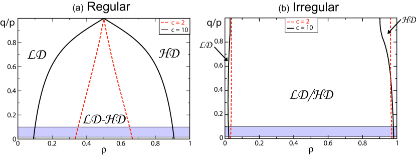
Figure 23: The stationary state of PASEP through regular graphs (a) and irregular graphs (b) are compared. The colour band presents a fraction $q/p\sim 2-10\%$ as have been measured in experiments on single kinesin-I motors [83, 84, 85]. We see that in general bi-directionality of motors does not substantially alter the heterogeneities in motor densities.

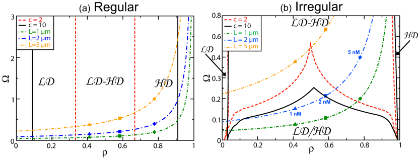
Figure 24: Illustration of the possible variation of the stationary state for kinesin-8 motors of budding yeast moving along a network of microtubules. We have plotted the exchange parameter $\Omega$ as a function of the total density $\rho$ based on numbers from [17] for given values of the length $L$ between two microtubule intersections. These lines are plotted on the diagrams of TASEP-LK on regular networks (a) (from figure 18) and irregular networks (b) (from figure 20). The markers denote the values of $(\Omega,\rho)$ for given values of $L$ and the total concentration $c_{m}$ of motors in the solution (triangles correspond to $1nM$, squares to $2nM$ and diamonds to $5nM$).

Second, we turn to the question of finite motor processivity. In figure 24 we indicate reasonable parameter values as estimated from in-vitro experiments on the diagrams for the stationary state of TASEP-LK on regular and irregular networks, figures 18 and 20. To make this educated guess at the biological relevant regime of the parameters $\Omega$ and $\rho$, we consider the in-vitro experiments by Varga et al. [16] and by Leduc et al. [17], which concern the transport of the kinesin-8 motor of budding yeast (Kip3P) along microtubules. Kip3P is an interesting motor in our context, since its dynamics on a single microtubule are well described by TASEP-LK [17]. Kip3 depolymerizes tubulin dimers at the plus end of the microtubules, and recently an extension of this model has yielded insight into the role of active transport in depolymerizing filaments [89, 90]. The microscopic parameters of Kip3P, due to this particular biological function, might be different from that of other kinesins, but this does not alter the qualitative picture of our results.

The parameters $\Omega$ and $\rho$ can be estimated from the data in [16], and such estimates have been considered before in the theoretical work [34]. To do so we exploit the functional relationship between $\Omega$ and $\rho$, which follows directly from the definitions as $\Omega(\rho)=\Omega_{D}/(2(1-\rho))$. It therefore only depends on the appropriately scaled detachment parameter $\Omega_{D}=\omega_{D}L/p$, which can be interpreted as the fraction of a segment in the network an isolated motor typically moves before detaching. For Kip3P we have $\omega_{D}/p\approx 7.5\>10^{-4}$, and the length of the microtubules is of the order $1-10\mu m$. Furthermore, taking the size of tubulin dimers to be about $8.4nm$ we obtain an estimated segment length of $L\sim 100-1000$.

In figure 24 we present the relation $\Omega=\Omega(\rho)$ at fixed $\Omega_{D}$, corresponding to three different segment lengths ($L=1\mu m$, $2\mu m$ and $5\mu m$), superposing it onto the phase diagram of TASEP-LK, for regular and irregular networks. The corresponding lines indicate how the state of the network will evolve as the total motor protein concentration $c_{m}$ in the solution is varied (note that we must distinguish the total motor protein concentration $c_{m}$ from the density $\rho$ of bound motors on the network: $c_{m}$ is the ratio of the total number of motors to the volume of the solution, whereas $\rho$ is the ratio of the number of bound motors to the number of tubulin dimers on the cytoskeleton). Recall also that the overall density of bound motors is $\rho=K/(K+1)$, with $K=\tilde{\omega}_{A}c_{m}/\omega_{D}$, assuming an infinitely large and homogeneous reservoir. Using the estimates $\tilde{\omega}_{A}\approx 3.3\>10^{-3}nM^{-1}s^{-1}$, $c_{m}=1nM$, $2nM$ or $5nM$ and $\omega_{D}=4.7\>10^{-3}s^{-1}$, as given in [16], we can position the state of the system at the markers in figure 24.

We can draw several interesting conclusions from figures 24. First, we see that the biological parameters are such that all the different regimes of density heterogeneities can be reached, and can in fact be targeted for instance by varying the total motor protein density $c_{m}$ or by varying the number $L$ of tubulin dimers between two junctions. In cells the segment length $L$ can be regulated in various ways, for instance by varying the concentration of crosslinker proteins, a small value of $L$ corresponding to high crosslinker concentrations. Second, the network topology is important for this regulation. As the density of motor proteins on the network varies its mapping onto the $(\rho,\Omega)$ plane swepdf out lines, as discussed above, and which are set by the segment length $L$ and motor properties (rates $p$ and $\omega_{D}$). Several examples are indicated in figures 24. For regular networks, the choice of these parameters always leads to the same succession of transitions between regimes of heterogeneity. This is different for irregular network topologies, for which increasing $L$ (or $\Omega_{D}$) beyond a threshold value circumvents the $\mathcal{LD/HD}$ regime altogether. Consequently, these estimates show that cells could indeed exploit heterogeneities associated with the stationary transport regimes in order to regulate the overall organization of matter along the cytoskeleton.

7 Conclusion

In this work we have studied driven lattice gases through networks. These systems form a class of minimal models for intracellular transport of motor proteins along the cytoskeleton. Motor proteins are considered to be active particles which move stochastically along a complex network and the cytoskeleton is modeled as a network of one-dimensional lattices which interconnect at junction sites. Three main results on which we report in this conclusion follow from our study.

One of the main insights of this work is that the stationary state of transport processes on networks can be deduced from the phase diagram of a single open segment connecting two particle reservoirs. Indeed, using mean field arguments we can characterize the stationary state of each segment in the network using effective entry and exit rates. Plotting the effective rates of all segments on the single-segment phase diagram we can represent the stationary state of the whole network. This approach leads naturally to the classification of the stationary state of excluded volume processes in three distinct regimes:

• homogeneous regime ($\mathcal{LD}$ or $\mathcal{HD}$): all segments are in the same homogeneous phase, i.e. either the LD or HD phase. As a consequence, the particles are distributed homogeneously along the network. TASEP, PASEP and TASEP-LK on regular graphs all occupy this regime at low and high filling of particles on the network. On irregular graphs this regime can only appear at very low or very high particle densities.

• heterogeneous segment regime ($\mathcal{LD-HD}$): this regime is dominated by segments occupying the LD-HD phase. As a consequence, strong density heterogeneities are present within single segments. TASEP, PASEP and TASEP-LK on regular graphs occupy this regime at intermediate particle filling. For irregular graphs this regime appears at low processivity (i.e. high values of the exchange rate $\Omega$).

• heterogeneous network regime ($\mathcal{LD/HD}$): a finite fraction of segments are in the LD phase but another finite fraction of segments are in the HD phase. Therefore, a part of the network is sparcely occupied with particles, whereas another part has a very high occupancy. Strong heterogeneities are present on a network scale. This regime appears naturally on irregular graphs in TASEP, PASEP and TASEP-LK with high processivity.

To which of these three regimes the stationary state corresponds thus depends on the topology of the network, on the microscopic nature of the transport process and on the “molecular“ parameters of the particles. Having reduced the problem of studying transport along a complex network to the properties of one-dimensional transport is a considerable simplification also in practical terms: a large number of exact and approximative, established over the last two decades on one-dimensional lattice gases [30, 35], can be directly exploited. When studying transport processes other than TASEP it might be necessary to define other network regimes than the one presented here, which can also be constructed from the one-dimensional phase diagram of the corresponding transport process.

A second main insight of our work is that strong heterogeneities on a network are a robust feature of non-equilibrium transport with exclusion interactions. Therefore, we expect it to be relevant in the study of real transport processes such as motor protein transport along the cytoskeleton (or vehicular traffic in a city, etc.). The occurrence of a network regime can be understood clearly from the effective rate diagrams as a consequence of two effects: the presence of a LD and a HD phase, separated by a first order transition, on one hand, in one-dimensional transport, and the presence of any kind of ’quenched’ disorder on the other hand which affects the currents at the junction sites. For instance, microtubules may present local changes, due to post-translational modifications, to the absorption of proteins on the microtubule substrate [12] or to the generation of microtubules by augmin protein complexes [91]. Any such disorder leads to a scattering of the effective rates with respect to the one-dimensional phase diagram (see figures 5, 9 and 16). This results in a part of the segments being in a LD state and another part being in a HD state. These arguments can be extended to a large number of transport problems for which the one-dimensional phase diagram is known [35], for which we only mention a few examples relevant to motor protein transport: TASEP with extended particles [74], TASEP with synchronuous dynamics [76], TASEP with multiple lanes [77, 78, 79, 80], TASEP with particles with internal states [33, 41], TASEP with directional switching [82], etc. Furthermore, our argument applies irrespectively of the origin of the disorder in the effective rates. Here we were interested in the effect of irregularity of the graph architecture, but the effective rates can also capture disorder in the way particles move at the junction sites, the spatial clustering of filaments, etc. Our insights into the appearance of network heterogeneities in the particle distributions apply therefore far beyond the specific Erdös-Rényi graphs we have considered here.

A third result of our work is physical insight into how heterogeneities appear in equilibrium transport processes when these are gradually driven out of equilibrium. To resolve this question we have interpolated between a passive process, in which particles diffuse bi-directionally on the network, and an active process, in which they move uni-directionally. We have interpolated between these two limiting cases by gradually changing the bias in the directionality of the particles. Analyzing the stationary state using our effective rate diagram approach has revealed that, for sufficiently large systems, even a weak preference for one direction suffices to create strong density heterogeneities. We have also considered active transport along a network with coupling to passive bulk diffusion in a reservoir. Varying the exchange rate we can again interpolate between an equilibrium diffusive process and an active transport process along a network [53]. When the exchange is small, the active process leads to a heterogeneous network regime as in TASEP. Increasing the exchange rate further makes the network heterogeneities disappear. The stationary state corresponds then to a segment regime with heterogeneities at the segment level. Eventually, when the exchange rate becomes very high, the exchange process smoothens out all heteroeneities and particles are distribute homogeneously over the network.

On biological grounds, since motor proteins play a key role in creating gradients within cells, but are also involved in force production and regulation as well as the control of filament length in cells. Understanding how motor proteins organize along the cytoskeleton therefore constitutes an essential element in the study of the microscopic statistical physics of biological cells. We have shown that the different regimes of density heterogeneities of TASEP-LK through networks could be relevant to cellular processes, as these regimes arise for parameter values which are consistent with estimates from in-vitro experiments on motor proteins. In particular, our results indicate that density heterogeneities on irregular networks could be regulated via various parameters such as motor processivity, crosslinker density or the bulk concentration of motors.

Appendix A Current and density profiles for TASEP-LK for a single segment

In this appendix we revisit the current and density profiles for TASEP-LK on a single segment, as they have been determined from mean-field arguments in the literature [58, 59]. In the hydrodynamic limit the mean-field equation for the average density $\rho^{\rm LK}(x)$ reads:

$$(2\rho-1)\partial_{x}\rho^{\rm LK}=\Omega_{A}(1-\rho^{\rm LK})-\Omega_{D}\rho^{\rm LK}.$$ (50)

We first consider the limiting case $K=1$ ($K=\Omega_{A}/\Omega_{D}$), which admits linear analytical solutions for the density profiles. We then consider the general case $K\neq 1$, which is more representative to real situations but also more technical: the density profiles are given by the different branches of the real Lambert W function [59]. We end our discussion with several analytical results with respect to the phase diagram of TASEP-LK.

A.1 Special case of half-filling: $\Omega_{A}=\Omega_{D}$

Let us first consider the case $K=1$, corresponding to half-filling ($\rho=1/2$), for which the continuity equation (50) simplifies considerably and leads to piecewise linear density profiles. In order to match the boundary conditions we must distinguish two cases, depending on the values of two parameters $x_{\alpha},x_{\beta}\in[0,1]$ corresponding to positions along the segment:

$$x_{\alpha} = \Omega^{-1}\left(1/2-\frac{\alpha}{p}\right),$$ (51)

$$x_{\beta} = 1+\Omega^{-1}\left(\frac{\beta}{p}-1/2\right).$$ (52)

Depending on the relative positions $x_{\alpha}$ and $x_{\beta}$ the density is given by

$$\rho^{\rm LK}\left[x;\alpha,\beta,\Omega_{A},\Omega_{D}\right]=\left\{\begin{array}[]{cclcc}\rho_{\alpha}&=&\Omega\>x+\frac{\alpha}{p}&x<x_{\alpha}&{\rm(LD)}\\ \rho_{l}&=&1/2&x_{\beta}<x<x_{\alpha}&{\rm(MC)}\\ \rho_{\beta}&=&\Omega\>(x-1)+1-\frac{\beta}{p}&x>x_{\beta}&{\rm(HD)}\end{array}\right.,$$ (56)

when $x_{\alpha}<x_{\beta}$ and by

$$\rho^{\rm LK}\left[x;\alpha,\beta,\Omega_{A},\Omega_{D}\right]=\left\{\begin{array}[]{cclcc}\rho_{\alpha}&=&\Omega\>x+\frac{\alpha}{p}&\qquad x<x_{w}&{\rm(LD)}\\ \rho_{\beta}&=&\Omega\>(x-1)+1-\frac{\beta}{p}&\qquad x>x_{w}&{\rm(HD)}\end{array}\right.,$$ (59)

when $x_{\alpha}>x_{\beta}$. The variable $x_{w}$ denotes the position of the domain wall in the segment and is given by:

$$x_{w} = \frac{1}{2\Omega}\,\left(\frac{\beta-\alpha}{p}+\Omega\right).$$ (60)

From the phase diagram for TASEP-LK (see figure 25) we see that in addition to LD, HD and MC phases it also contains zones corresponding to the composite LD-HD, LD-MC, MC-HD and LD-MC-HD phases. As $\Omega$ increases, the MC phase progressively dominates the phase diagram. This is not surprising, since here the MC phase is the equilibrium state corresponding to the homogeneous density $\rho_{\ell}=\Omega_{A}/(\Omega_{D}+\Omega_{A})=1/2$ set by the reservoir.

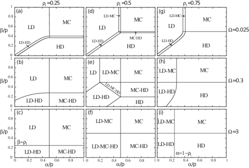
Figure 25: The $(\alpha/p,\beta/p)$-phase diagram for TASEP-LK on a single segment for the indicated values of $\Omega$ and $\rho_{ell}=K/(K+1)$. For $\Omega\rightarrow 0$ we recover the TASEP phase diagram with the homogeneous LD, HD and MC phases. For increasing values of $\Omega$ the heterogeneous LD-HD phase, which was restricted to a coexistence line for $\Omega=0$, grows and plays a more prominent role. The analytical expressions for the phase transitions for large $\Omega$ are also indicated.

A.2 General case: $\Omega_{A}\neq\Omega_{D}$

We now turn to the general case where $K\neq 1$. Here we first consider $K>1$, corresponding to a HD Langmuir phase ($\rho_{l}>1/2$). The case $K<1$ follows readily from the solution for $K>1$ by exploiting the particle-hole symmetry. The two systems are related by the following transformation:

$$K\rightarrow 1/K,\ (\alpha,\beta)\rightarrow(\beta,\alpha),\ x\rightarrow 1-x\ \mbox{and}\ \rho\rightarrow 1-\rho.$$ (61)

We define the rescaled density $\sigma[x]$ through

$$\sigma[x]\equiv\frac{K+1}{K-1}\left(2\rho[x]-1\right)-1,$$ (62)

such that the Langmuir density is given by $\sigma=0$. It is independent of $K$.

We define the two functions

$$Y_{\alpha}[x] = \left|\sigma[0]\right|\exp\left[2\Omega\frac{(K+1)}{(K-1)}x+\sigma[0]\right],$$ (63)

$$Y_{\beta}[x] = \left|\sigma[1]\right|\exp\left[2\Omega\frac{(K+1)}{(K-1)}(x-1)+\sigma[1]\right].$$ (64)

The boundary conditions, $\rho[0]=\alpha/p$ and $\rho[1]=1-\beta/p$ determine $\sigma[0]$ and $\sigma[1]$. The solution for the profiles $\sigma[x]$ are given in terms of the two branches $W_{-1}$ and $W_{0}$ of the real-valued Lambert $W$ function. We find the left boundary solution

$$\sigma_{\alpha}[x]=W_{-1}\left[-Y_{\alpha}[x]\right]<-1,$$ (65)

corresponding to a density $\rho_{\alpha}<1/2$ and the right boundary solution

$$\sigma_{\beta}[x]=\left\{\begin{array}[]{ccc}W_{0}\left[Y_{\beta}[x]\right]>0&&0\leq\beta<p(1-\rho_{\ell})\\ 0&&\beta=p(1-\rho_{\ell})\\ W_{0}\left[-Y_{\beta}[x]\right]<0&&p(1-\rho_{\ell})<\beta\leq p/2\\ W_{0}\left[-Y_{1/2}[x]\right]<0&&\beta>p/2\end{array}\right..$$ (70)

Note that the left boundary solution is only defined for values of $x$ such that $Y_{\alpha}[x]<1/e$. The two solutions are matched at the position $x_{w}\in[0,1]$, for which the current of both solutions are equal: $\rho_{\alpha}[x_{w}]=1-\rho_{\beta}[x_{w}]$. If $x_{w}\in[0,1]$ we are in the LD-HD phase (or the LD-MC phase when $\beta>p/2$). Otherwise we are in a LD, HD or MC phase, depending on the solution which dominates the current. The MC phase corresponds to the boundary independent solution $W_{0}\left[-Y_{1/2}[x]\right]$ and appears for $\beta>p/2$. Here (for $K>1$) MC has a density larger than one half. All phases here generalize the equivalent homogeneous phases in TASEP.

We can now evaluate the solution in the various quadrants of the $(\alpha/p,\beta/p)$ phase diagram:

• $\alpha/p<1/2$ and $\beta/p<1/2$: in this case one can have either LD, LD-HD or HD phases, depending on the position of the domain wall $x_{w}$.

• $\alpha/p<1/2$ and $\beta/p>1/2$: one can have the LD, LD-MC or MC phase. Again, one has to calculate the position $x_{w}$ of the domain wall. The right boundary solution is given by $W_{0}\left[-Y_{1/2}[x]\right]$, independently of $\beta$. For $x_{w}<0$ we obtain the boundary independent MC phase. We also remark that here the LD-MC phase has the particularity that the MC part is boundary (i.e. $\beta$) independent.

• $\alpha/p>1/2$ and $\beta/p<1/2$: the system is in the HD phase.

• $\alpha/2>1/2$ and $\beta/p>1/2$: the system is in the MC phase.

The phase diagrams in figure 25 are constructed as follow: the transition between LD and LD-HD phases (and LD and LD-MC for $\beta/p>1/2$) follows from the condition $x_{w}=1$. Analogously, the transition between the LD-HD and HD (or MC) phases follows from the condition $x_{w}=0$. The transition between the HD and MC phases is given by $\beta/p=1/2$. For $\beta/p>1/2$ all transition lines are vertical independent of $\beta$.

At low values of $\Omega$ the phase diagram involves four phases, i.e. the LD, HD, MC, LD-HD and LD-MC phase. When increasing the exchange rate $\Omega$ the LD phase becomes gradually smaller and eventually disappears at a critical value $\Omega_{c}$:

$$\Omega_{c}=\frac{K-1}{2(K+1)}\left(-1+\ln\left(\frac{K-1}{2K}\right)+\frac{2K}{K-1}\right).$$ (71)

A.3 The phase diagram of TASEP-LK at $\Omega\rightarrow\infty$

The phase diagram of TASEP-LK is represented in figure 25. In general we have no explicit analytical expressions for the TASEP-LK phase diagram, but we do have the explicit expression for the phase diagram at $\Omega\rightarrow\infty$. Let us elaborate on three different cases:

• $K>1$: such that the Langmuir density $\rho_{\ell}>1/2$ corresponds to a HD phase.

  • LD-HD: $\alpha/p<1-\rho_{\ell}$ and $\beta/p<1/2$

  • LD-MC: $\alpha/p<1-\rho_{\ell}$ and $\beta/p>1/2$

  • HD: $\alpha/p>1-\rho_{\ell}$ and $\beta/p<1/2$

  • M: $\alpha/p>1-\rho_{\ell}$ and $\beta/p>1/2$

• $K<1$, such that the Langmuir density $\rho_{\ell}<1/2$ corresponds to a LD phase. The phase diagram follows readily from that for $K>1$ using the particle-hole symmetry transformations given above.

• $K=1$ is a special situation, as then the Langmuir density $\rho_{\ell}=1/2$ corresponds to half filling. The Langmuir phase thus corresponds to the MC phase. For $K=1$ a part of the segment will reach this Langmuir phase (which for $K\neq 1$ is only the case in the limit $\Omega\rightarrow\infty$). This leads to the LD-MC-HD, LD-MC and MC-HD phases. Due to the linear density profiles at $K=1$ one can determine explicitly analytic expressions for the phase diagram [59], which is presented in figure 25. For values of $\Omega_{c}>1/2$ (which follows from equation (71)) the phase diagram is given by the simple expression

  • LD-HD or LD-MC-HD: $\alpha/p<1/2$, $\beta/p<1/2$

  • MC-HD: $\alpha/p>1/2$ and $\beta/p<1/2$

  • LD-MC: $\alpha/p<1/2$ and $\beta/p>1/2$

  • MC: $\alpha/p>1/2$ and $\beta/p>1/2$

  The LD-HD phase is not present for $\Omega>1$.

Appendix B Universal expression for networks with infinite connectivity

We present here the analytical and universal expression for the current-density profile of infinitely connected graphs ($c\rightarrow\infty$). The first observation is that the approximate mean field equations (40) are seen to become exact in the infinitely connected limit. As discussed in section 5.4, the infinite connectivity limit amounts to considering all junctions blocked: $\rho_{v}=1$ for all junctions.

This is reflected in the effective rates which scale with the average connectivity $c$ as $(\alpha^{\rm eff},\beta^{\rm eff})\sim(\mathcal{O}(c^{-1}),\mathcal{O}(c^{-1}))$, and therefore the expression for the current follows from the TASEP-LK single segment current by setting $(\alpha/p,\beta/p)=(0,0)$. For mean densities on the network $\rho>1/2$ we obtain (using $\rho=K/(1+K)$)

$$J/p = \int^{x_{w}}_{0}\>\rho^{\infty}_{\alpha}\left[x\right]\left(1-\rho^{\infty}_{\alpha}\left[x\right]\right)dx+\int^{1}_{x_{w}}\rho^{\infty}_{\beta}\left[x\right]\left(1-\rho^{\infty}_{\beta}\left[x\right]\right)dx$$ (72)

$$= \rho-\int^{x_{w}}_{0}\>\left(\rho^{\infty}_{\alpha}\left[x\right]\right)^{2}dx-\int^{1}_{x_{w}}\left(\rho^{\infty}_{\beta}\left[x\right]\right)^{2}dx$$

with $x_{w}$ the domain wall position defined through the condition $\rho^{\infty}_{\alpha}\left(x_{w}\right)=1-\rho^{\infty}_{\beta}\left(x_{w}\right)$, and

$$\sigma^{\infty}_{\alpha}\left[x\right] = W_{-1}\left[-\frac{2\rho}{2\rho-1}\exp\left[\frac{2\left(\Omega\>x-\rho\right)}{2\rho-1}\right]\right],$$ (73)

$$\sigma^{\infty}_{\beta}\left[x\right] = W_{0}\left[\frac{2(1-\rho)}{2\rho-1}\exp\left[\frac{2\left(\Omega(x-1)+(1-\rho)\right)}{2\rho-1}\right]\right].$$ (74)

We have $\sigma^{\infty}_{\alpha/\beta}[x]=(2\rho^{\infty}_{\alpha/\beta}[x]-1)/(2\rho-1)-1$. For $\rho<1/2$ we can deduce the analoguous expressions from particle-hole symmetry $(\rho\rightarrow 1-\rho)$, while for the special case $\rho=1/2$ the integrals in equation (72) can be integrated explicitly to find the expression in C.

Appendix C Half-filling for TASEP-LK on a network

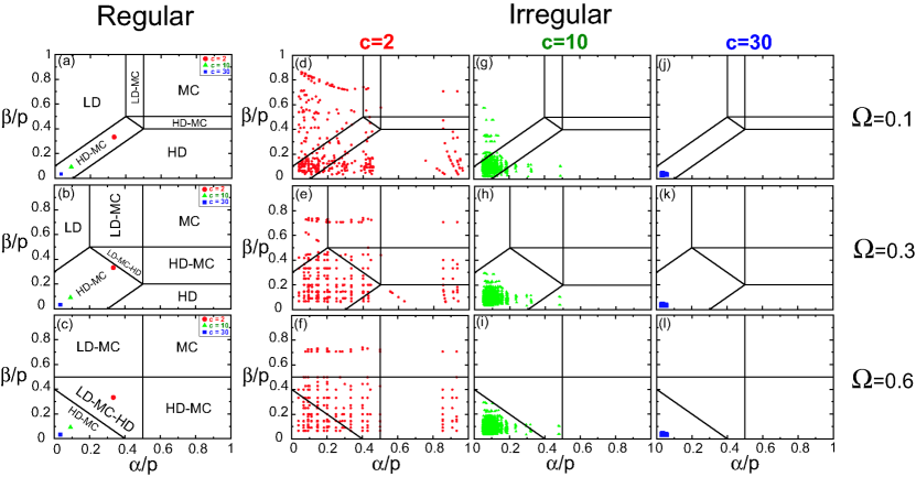
Figure 26: Effective rate diagrams for TASEP-LK through regular graphs (left) and irregular graphs (right), both at a total density of $\rho=1/2$, are presented for the given values of $\Omega$ and $c$. We have used the same graph instances as in figure 16. On regular networks the effective rates are equal for all segments, such that only one marker is plotted.

The case of half-filling ($\rho=1/2$, corresponding to $K=1$) mathematically simplifies TASEP-LK on a single segment since the density profiles are piecewise linear functions (see A). The corresponding phase diagrams are known analytically, see figure 25 (d)-(f), and we exploit them for the effective rate diagrams for networks at half filling (figure 26). Using these results we now derive several simple analytical results on the scale of the network.

Infinite connectivity ($c\rightarrow\infty$) at half-filling

At infinite connectivity the effective rates cluster close to the origin, see figure 26. All segments decouple and become equivalent to isolated open segments with $\alpha^{\rm eff},\beta^{\rm eff}=(0,0)$. We recover the expressions in B. For $K=1$ we can explicitly integrate equation (72) to find

$$J/p=\left\{\begin{array}[]{cccc}\Omega/4-\Omega^{2}/12,&&\Omega<\Omega^{\ast}=1&{\mbox{(LD-HD)}}\\ 1/4-\Omega^{-1}/12,&&\Omega>\Omega^{\ast}=1&{\mbox{(LD-MC-HD)}}\end{array}\right.$$ (77)

We see that beyond some critical exchange parameter ($\Omega>\Omega^{\ast}=1$) a part of the segment attains the Langmuir phase (i.e. here the MC phase, since $K=1$ corresponds to half-filling). Moreover, the current approaches its Langmuir value $J/p=1/4$ for rather small values of $\Omega$ already .

Regular networks at half-filling

The special case of half-filling also allows to derive analytical expressions for TASEP transport on regular networks. For regular networks all segments are equivalent and have the same effective rates given by equation (48) (see also figure 26). As stated in the main text, the current density profile can then be established from the formulas in A. However, to find the average current one still has to integrate the local expression $J^{\rm LK}[x]$ along the segment $x\in[0,1]$. In general this is difficult, but the integration can be performed explicitely for half-filling. Then the current profile becomes quadratic, and we find

$$\frac{J(\Omega)}{p}=\left\{\begin{array}[]{lll}\frac{c}{(c+1)^{2}}+\frac{\Omega}{4}\left(\frac{c-1}{c+1}\right)-\frac{\Omega^{2}}{12}&\qquad(\Omega<\Omega^{\ast}\mbox{ : LD-HD})\\ \frac{1}{4}-\frac{1}{\Omega}\,\frac{1}{12}\,\left(\frac{c-1}{c+1}\right)^{3}\left(1-\frac{2}{c+1}\right)^{2}&\qquad(\Omega>\Omega^{\ast}\mbox{ : LD-MC-HD})\end{array}\right.$$ (78)

This shows that the current saturates gradually to its maximal value of $1/4$ due to the appearance of a MC phase in the middle of the segments, which is present beyond a threshold for the exchange parameter, $\Omega>\Omega^{\ast}=(c-1)/(c+1)$. As $\Omega$ is increased further the homogeneous Langmuir phase is attained asymptotically through growth of the MC zone within the individual segments. Note that this mechanism, for which the Langmuir phase appears in the middle of the segment, is particular to the $K=1$ case.

References

References

- [1] B. Alberts, A. Johnson, J. Lewis, M. Raff, K. Roberts, and P. Walter, Molecular biology of the cell. Garland science, Taylor & Francis Group, 5 ed., 2008.
- [2] D. A. Fletcher and R. D. Mullins, “Cell mechanics and the cytoskeleton,” Nature, vol. 463, pp. 485–492, 2010.
- [3] T. Vignaud, L. Blanchoin, and M. Théry, “Directed cytoskeleton self-organization,” Trends in Cell Biology, pp. 1–12, 2012.
- [4] S. Ramaswamy, “The mechanics and statistics of active matter,” Annu. Rev. Condens. Matt. Phys., vol. 1, pp. 323–345, 2010.
- [5] M. C. Marchetti, J. F. Joanny, S. Ramaswamy, T. B. Liverpool, J. Prost, M. Rao, and R. A. Simha, “Soft active matter.” http://arxiv.org/abs/1207.2929, 2012.
- [6] J. Howard, Mechanics of Motor Proteins and the Cytoskeleton. Sinauer Associates, 2001.
- [7] R. D. Vale, “The molecular motor toolbox for intracellular transport,” Cell, vol. 112, pp. 467–480, 2003.
- [8] L. S. Goldstein, “Kinesin molecular motors: transport pathways, receptors, and human disease,” Proc. Natl. Acad. Sci. U S A, vol. 98, pp. 6999–7003., 2001.
- [9] N. Hirokawa, Y. Noda, Y. Tanaka, and S. Niwa, “Kinesin superfamily motor proteins and intracellular transport,” Nature Reviews Molecular Cell Biology, vol. 10, pp. 682–696, 2009.
- [10] M. J. Schnitzer, K. Visscher, and S. M. Block, “Force production by single kinesin motors,” Nature Cell Biology, vol. 2, pp. 718–723, 2000.
- [11] J. L. Ross, M. Y. Ali, and D. M. Warshaw, “Cargo transport: molecular motors navigate a complex cytoskeleton,” Curr. Opin. Cell Biol., vol. 20, pp. 41–47, 2008.
- [12] D. Cai, D. P. McEwen, J. R. Martens, E. Meyhofer, and K. J. Verhey, “High-density mapping of single-molecule trajectories with photoactivated localization microscopy,” PLoS Biol., vol. 7, p. e1000216, 2009.
- [13] P. Pierobon, S. Achouri, S. Courty, A. R. Dunn, J. A. Spudich, M. Dahan, and G. Capello, “Velocity, processivity, and individual steps of single myosin v molecules in live cells,” Biophysical Journal, vol. 96, pp. 4268–4275, 2009.
- [14] J. Yoo, T. Kambara, K. Gonda, and H. Higuchi, “Intracellular imaging of targeted proteins labeled with quantum dots,” Experimental Cell research, vol. 314, pp. 3563–3569, 2008.
- [15] S. Bálint, I. V. Vilanova, A. S. Álvarez, and M. Lakadamyali, “Correlative live-cell and superresolution microscopy reveals cargo transport dynamics at microtubule intersections,” Proc Natl Acad Sci U S A., vol. 110, pp. 3375–3380, 2013.
- [16] V. Varga, C. Leduc, V. Bormuth, S. Diez1, and J. Howard, “Kinesin-8 motors act cooperatively to mediate length-dependent microtubule depolymerization,” Cell., vol. 138, pp. 1174–1183, 2009.
- [17] C. Leduc, K. Padberg-Gehle, V. Varga, D. Helbing, S. Diez, and J. Howard, “Molecular crowding creates traffic jams of kinesin motors on microtubules,” Proc Natl Acad Sci U S A., vol. 109, p. 6100, 2012.
- [18] A. A. Nascimento, J. R. Roland, and V. I. Gelfand, “Pigment cells: a model for the study of organelle transport,” Annu. Rev. Cell Dev. Biol., vol. 19, pp. 469–491, 2003.
- [19] O. Medalia, I. Weber, A. S. Frangakis, D. Nicastro, G. Gerisch, and W. Baumeister, “Macromolecular architecture in eukaryotic cells visualized by cryoelectron tomography,” Science, vol. 298, pp. 1209–13, 2002.
- [20] K. Ben-Harush, T. Maimon, I. Patla, E. Villa, and O. Medalia, “Visualizing cellular processes at the molecular level by cryo-electron tomography,” Journal of Cell Science, vol. 123, pp. 7–12, 2010.
- [21] F. Fleischer, R. Ananthakrischnan, S. Eckel, H. Schmidt, J. Käs, T. Svitkina, V. Schmidt, and M. Beil, “Actin network architecture and elasticity in lamellipodia of melanoma cells,” New Journal of Physics, vol. 9, p. 420, 2007.
- [22] A. Reymann, J. Martiel, T. Cambier, L. Blanchoin, R. Boujemaa-Paterski, and M. Théry, “Nucleation geometry governs ordered actin network structures,” Nature Materials, vol. 9, pp. 827–32, 2010.
- [23] D. Portran, J. Gaillard, M. Vantard, and M. Thery, “Quantification of MAP and molecular motor activities on geometrically controlled microtubule networks,” Cytoskeleton, 2012.
- [24] F. Jülicher, A. Ajdari, and J. Prost, “Modeling molecular motors,” Rev. Mod. Phys., vol. 69, pp. 1269–1281, 1997.
- [25] P. Reimann, “Brownian motors: noisy transport far from equilibrium,” Phys. Rep., vol. 361, p. 57, 2002.
- [26] T. Guérin, J. Prost, P. Martin, and J.-F. Joanny, “Coordination and collective properties of molecular motors: theory,” Curr. Opin. Cell Biol., vol. 22, p. 14, 2010.
- [27] D. Chowdhury, A. Schadschneider, and K. Nishinari, “Physics of transport and traffic phenomena in biology: from molecular motors and cells to organisms,” Physics of Life Reviews, vol. 2, pp. 318–352, 2005.
- [28] F. Spitzer, “Interaction of markov processes,” Adv. in Math., vol. 5, p. 246, 1970.
- [29] H. Spohn, Large scale dynamics of interacting particles. Springer-Verlag, 1991.
- [30] G. M. Schutz, Exactly Solvable Models for Many-Body Systems far from Equilibrium, vol. 19 of Phase Transitions and Critical Phenomena, ch. 1. London: Academic, 2000.
- [31] C. T. MacDonald, J. H. Gibbs, and A. C. Pipkin, “Kinetics of biopolymerization on nucleic acid templates,” Biopolymers, vol. 6, pp. 1–5, 1968.
- [32] C. T. MacDonald and J. H. Gibbs, “Concerning the kinetics of polypeptide synthesis on polyribosomes,” Biopolymers, vol. 7, p. 707, 1969.
- [33] K. Nishinari, Y. Okada, A. Schadschneider, and D. Chowdury, “Intracellular transport of single-headed molecular motors kif1a,” vol. 95, p. 118101, 2005.
- [34] L. Reese, A. Melbinger, and E. Frey, “Crowding of molecular motors determine microtubule depolymerization,” Bioph. Journ., vol. 101, pp. 2190–2200, 2011.
- [35] T. Chou, K. Mallick, and R. K. P. Zia, “Non-equilibrium statistical mechanics: From a paradigmatic model to biological transport,” Reports on Progress in Physics, vol. 74, p. 116601, 2011.
- [36] K. Mallick, “Some exact results for the exclusion process,” J. Stat. Mech., p. P01024, 2011.
- [37] T. Chou and D. Lohse, “Entropy-driven pumping in zeolites and biological channel,” Phys. Rev. Lett., vol. 82, pp. 3552–3555, 1999.
- [38] T. Karzig and F. von Oppen, “Signatures of critical full counting statistics in a quantum-dot chain,” Phys. Rev. B, p. 045317, 2010.
- [39] A. Schadschneider, “Statistical mechanics of trafic flow,” Physica A, vol. 285, p. 101, 2001.
- [40] D. Helbing, “Traffic and related self-driven many-particle systems,” Rev. Mod. Phys., vol. 73, pp. 1067–1141, 2001.
- [41] L. Ciandrini, I. Stansfield, and M. C. Romano, “Ribosome traffic on mrnas maps to gene ontology: genome-wide quantification of translation initiation rates and polysome size regulation,” PLoS Computational Biology, vol. 9, p. e1002866, 2013.
- [42] G. Kirchoff, “Ueber die auflösung der gleichungen, auf welche man bei der untersuchung der linearen vertheilung galvanischer ströme geführt wird,” Ann. Phys. Chem, pp. 497–508, 1847.
- [43] L. Lovász, Random walks on graphs: a survey, vol. 2, pp. 353–397. János Bolyai Mathematical Society, 1996.
- [44] S. Klumpp and R. Lipowsky, “Active diffusion of motor particles,” Phys Rev Lett, vol. 95, p. 268102, 2005.
- [45] P. K. Trong, J. Guck, and R. E. Goldstein, “Coupling of active motion and advection shapes intracellular cargo transport,” Phys. Rev. Lett., vol. 109, p. 028104, 2012.
- [46] A. Kahana, G. Kenan, M. Feingold, M. Elbaum, and R. Granek, “Active transport on disordered microtubule networks: The generalized random velocity model,” Phys. Rev. E, vol. 78, p. 051912, 2008.
- [47] F. Nédélec, T. Surrey, and A. C. Maggs, “Dynamic concentration of motors in microtubule arrays,” Phys. Rev. Lett., vol. 86, pp. 3192–3195, 2001.
- [48] P. C. Bressloff and J. M. Newby, “Stochastic models of intracellular transport,” Rev. Mod. Phys., vol. 85, p. 135, 2013.
- [49] M. Klann, H. Koeppl, and M. Reuss, “Spatial modeling of vesicle transport and the cytoskeleton: The challenge of hitting the right road,” PLoS ONE, vol. 7, p. e29645, 2012.
- [50] P. Greulich and L. Santen, “Active transport and cluster formation on 2d networks,” Eur. Phys. J. E, vol. 32, p. 191, 2010.
- [51] T. Ezaki and K. Nishinari, “A balance network for the asymmetric simple exclusion process,” J. Stat. Mech., p. P11002, 2012.
- [52] I. Neri, N. Kern, and A. Parmeggiani, “The totally asymmetric simple exclusion process on networks,” Phys. Rev. Lett., vol. 107, p. 068702, 2011.
- [53] I. Neri, N. Kern, and A. Parmeggiani, “Modelling active transport and spatial-temporal organization of motor proteins along cytoskeleton,” Phys. Rev. Lett., vol. 110, p. 098102, 2013.
- [54] J. Krug, “Boundary-induced phase transitions in driven diffusive systems,” Phys. Rev. Lett., vol. 67, pp. 1882–1885, 1991.
- [55] B. Derrida, M. R. Evans, V. Hakim, and V. Pasquier, “Exact solution of a 1d asymmetric exclusion model using a matrix formulation,” J. Phys. A: Math. Gen., vol. 26, p. 1493, 1993.
- [56] B. Derrida, E. Domany, and D. Mukamel, “An exact solution of the one dimensional asymmetric exclusion model with open boundaries,” J. Stat. Phys., vol. 69, pp. 667–687, 1992.
- [57] S. Sandow, “Partially asymmetric exclusion process with open boundaries,” Phys. Rev. E, vol. 50, pp. 2660–2667, 1994.
- [58] A. Parmeggiani, T. Franosch, and E. Frey, “Phase coexistence in driven one-dimensional transport,” Phys. Rev. Lett., vol. 90, p. 086601, 2003.
- [59] A. Parmeggiani, T. Franosch, and E. Frey, “The totally asymmetric simple exclusion process with langmuir kinetics,” Phys. Rev. E, vol. 70, p. 046101, 2004.
- [60] J. Howard, “Molecular motors: structural adaptations to cellular functions,” Nature, vol. 389, pp. 561–567, 1997.
- [61] H. Lodish, A. Berk, S. L. Zipursky, P. Matsudaira, D. Baltimore, and J. Darnell, Molecular Cell Biology. W. H. Freeman, 2000.
- [62] B. Bollobás, Random graphs. Cambridge University Press, 2001.
- [63] H. A. Bethe, “Statistical theory of superlattices,” Proc. Roy. Soc. London Ser A, vol. 150, pp. 552–575, 1935.
- [64] R. J. Baxter, Exactly solved models in statistical mechanics, ch. 4. Academic Press, 1982.
- [65] E. N. Gilbert, “Random graphs,” Annals of Math. Stat., vol. 30, pp. 1141–1144, 1959.
- [66] P. Erdös and A. Rényi, “On the evolution of random graphs,” Publications of the Mathematical Institute of the Hungarian Academy of Sciences, vol. 5, p. 17–61, 1960.
- [67] R. E. Tarjan, “Depth-first search and linear graph algorithms,” SIAM J. Comput., vol. 1, pp. 146–160, 1972.
- [68] A. Barrat, M. Barthélemy, and V. Vespignani, Dynamical Processes on Complex Networks. Cambridge University Press, 2008.
- [69] M. E. J. Newman, Networks, An Introduction. Oxford University Press, 2010.
- [70] B. Embley, A. Parmeggiani, and N. Kern, “Understanding totally asymmetric simple-exclusion-process transport on networks: generic analysis via effective rates and explicit vertices.,” Phys. Rev. E, vol. 80, p. 041128, 2009.
- [71] A. Raguin, N. Kern, and A. Parmeggiani in preparation, 2012.
- [72] G. Schutz and E. Domany, “Phase transitions in an exactly soluble one-dimensional exclusion process,” J. Stat. Phys., vol. 72, p. 277, 1993.
- [73] A. B. Kolomeisky, G. M. Shütz, E. B. Kolmeisky, and J. P. Straley, “Phase diagram of one-dimensional driven lattice gases with open boundaries,” J. Phys. A: Math. Gen., vol. 31, pp. 6911–6919, 1998.
- [74] L. B. Shaw, R. K. P. Zia, and K. H. Lee, “Totally asymmetric exclusion process with extended objects: A model for protein synthesis,” Phys. Rev. E, vol. 68, p. 021910, 2003.
- [75] P. Pierobon, E. Frey, and T. Franosch, “Driven lattice gas of dimers coupled to a bulk reservoir,” Phys. Rev. E, vol. 74, p. 031920, 2006.
- [76] L. G. Tilstra and M. H. Ernst, “Synchronous asymmetric exclusion processes,” J. Phys. A: Math. Gen., vol. 31, p. 5033, 1998.
- [77] E. Pronina and A. B. Kolomeisky, “Two-channel totally asymmetric simple exclusion processes,” J. Phys. A: Math. Gen., vol. 37, pp. 9907–9918, 2004.
- [78] T. Reichenbach, E. Frey, and T. Franosch, “Traffic jams induced by rare switching events in two-lane transport,” New. J. Phys., vol. 9, p. 159, 2007.
- [79] C. Schiffmann, C. Appert-Rolland, and L. Santen, “Shock-dynamics of two-lane driven lattice gases,” J. Stat. Mech., p. P06002, 2010.
- [80] M. R. Evans, Y. Kafri, K. E. P. Sugden, and J. Tailleur, “Phase diagram of two-lane driven diffusive systems,” J. Stat. Mech., p. P06009, 2011.
- [81] L. Ciandrini, M. C. Romano, and A. Parmeggiani, “Cooperative phenomena in biological transport: A theorist’s perspective.” 2013.
- [82] S. Muhuri, L. Shagolsem, and M. Rao, “Bidirectional transport in a multispecies totally asymmetric exclusion-process model,” Phys Rev E, vol. 84, p. 031921, 2011.
- [83] M. J. Schnitzer and S. M. Block, “Kinesin hydrolyses one atp per 8-nm step,” Nature, vol. 388, pp. 386–390, 1997.
- [84] H. Kojima, E. Muto, H. Higuchi, and T. Yanagida, “Mechanics of single kinesin molecules measured by optical trapping nanometry,” Biophysical Journal, vol. 73, pp. 2012–2022, 1997.
- [85] K. Visscher, M. J. Schnitzer, and S. M. Block, “Single kinesin molecules studied with a molecular force clamp,” Nature, vol. 400, pp. 184–189, 1998.
- [86] M. A. Welte, “Bidirectional transport along microtubules,” Curr. Biol., vol. 14, pp. R525–R537, 2004.
- [87] S. P. Gross, “Hither and yon: a review of bi-directional microtubule-based transport,” vol. 1, pp. R1–R11, 2004.
- [88] R. Fowler, Statistical Mechanics. Cambridge University Press, 1936.
- [89] A. Melbinger, L. Reese, and E. Frey, “Microtubule length regulation by molecular motors,” Phys. Rev. Lett, vol. 108, p. 258104, 2012.
- [90] D. Johann, C. Erlenkämper, and K. Kruse, “Length regulation of active biopolymers by molecular motors,” Phys. Rev. Lett, vol. 108, p. 258103, 2012.
- [91] S. Petry, C. Pugieux, F. Nedelec, and R. Vale, “Augmin promotes meiotic spindle formation and bipolarity in xenopus egg extracts,” Proc. Natl. Acad. Sci. U S A, vol. 108, pp. 14473–14478, 2011.