Distinct Degrees and Their Distribution in Complex Networks

Abstract

We investigate a variety of statistical properties associated with the number of distinct degrees that exist in a typical network for various classes of networks. For a single realization of a network with $N$ nodes that is drawn from an ensemble in which the number of nodes of degree $k$ has an algebraic tail, $N_{k}\sim N/k^{\nu}$ for $k\gg 1$, the number of distinct degrees grows as $N^{1/\nu}$. Such an algebraic growth is also observed in scientific citation data. We also determine the $N$ dependence of statistical quantities associated with the sparse, large-$k$ range of the degree distribution, such as the location of the first hole (where $N_{k}=0$), the last doublet (two consecutive occupied degrees), triplet, dimer ($N_{k}=2$), trimer, etc.

1 Introduction

A complete microscopic representation of a macroscopic system is usually unavailable and often unnecessary, especially if the system is evolving or it is taken from an ensemble and the goal is to understand the typical features of the ensemble. Thus instead of determining a huge number of parameters (such as the $10^{23}$ coordinates and momenta of atoms), it often suffices to know a few useful macroscopic quantities (like the total number of atoms and the total energy) to understand the bulk properties of a macroscopic system.

In the realm of networks, one usually starts with an ensemble of large networks that are generated according to a specified and not completely deterministic algorithm. In analogy with other bulk systems, we are typically interested in macroscopic-like network characteristics, such as the total number of links, the total number of triangles, the total number of clusters (maximal connected components), etc. [1]. Two of the most useful macroscopic characteristics are the cluster-size distribution and the degree distribution.

The degree of a node (the number links attached to the node) is perhaps the simplest local network characteristic. It has been now been extensively studied, with an emphasize on networks with broadly distributed degrees [2]. Here we analyze the number of distinct degrees $D_{N}$ that exists for a given network of size $N$. The number $D_{N}$ varies from realization to realization, but for the ensembles that we study $D_{N}$ turns out to be a self-averaging quantity, so that its mean value is the most important characteristic. We focus on $\langle D_{N}\rangle$ which we generally write as $D_{N}$ when no ambiguity is possible.

We also investigate the locations of the first hole (the smallest $k$ where $N_{k}$ equals zero), the last doublet (the largest $k$ value for which $N_{k}>0$ and $N_{k+1}>0$), last triplet, the last dimer (the largest $k$ value where $N_{k}=2$), trimer, etc. in the degree distribution (Fig. 1).

Figure 1: A network of 16 nodes, with node degrees indicated. In this example, $N_{k}=\{7,4,1,0,2,1,0,1\}$. The number of distinct degrees $D_{16}=6$, the last doublet occurs at $k=5$, the last dimer also at $k=5$, the first hole at $k=4$, and $k_{\rm max}=8$.

The number of distinct degrees $D_{N}$ exhibits interesting behavior for network ensembles in which the degree distribution has an algebraic tail; hence we focus on such networks. For concreteness, we consider networks that are grown by preferential attachment. The best-known case is strictly linear preferential attachment [3, 4, 5, 6, 7, 8], in which a new node attaches to a pre-existing node of degree $k$ with rate $A_{k}=k$. To illustrate the quantities studied here, we plot the degree distribution for a realization of such a network of $N=10^{7}$ nodes (Fig. 2). For small $k$, every degree is represented, that is, $N_{k}>0$. As $k$ increases, eventually a point is reached where $N_{k}$ first equals zero; this defines the first “hole” in the degree distribution. Holes become progressively more common for larger $k$ and eventually the distribution becomes sparse. Figure 2 also indicates the position of the last doublet, the largest $k$ for which $N_{k}>0$ for two consecutive $k$ values, while the last dimer is defined as the largest $k$ value for which $N_{k}=2$. One can analagously define the last triplet and last trimer, etc. As $k$ continues to increase, the degree distribution is non-zero at progressively more isolated $k$ values and eventually the distribution terminates when largest network degree $k_{\rm max}$ is reached.

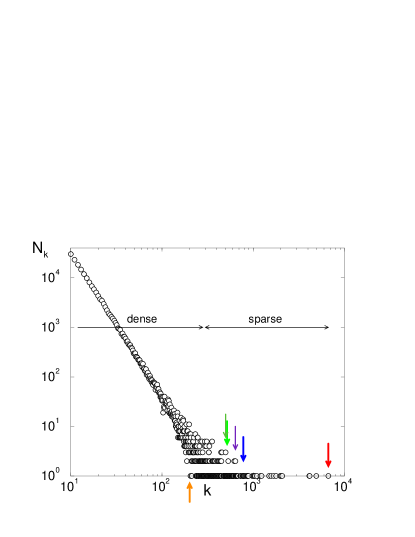
Figure 2: Number of nodes of degree $k\geq 10$ for a single network realization of $N=10^{7}$ nodes that is grown by strictly linear preferential attachment. The largest degree is $k_{\rm max}=6693$, $D_{N}=465$, the last doublet occurs at $k=782$, the last dimer at $k=641$, the last triplet at $k=518$, the last trimer at $k=500$, and the first hole at $k=201$ (arrows).

One of our principal results is that

$$D_{N}\simeq\Gamma\big{(}1-\tfrac{1}{\nu}\big{)}\,(RN)^{1/\nu}$$ (1)

for networks whose degree distribution has the algebraic tail

$$N_{k}\simeq NRk^{-\nu}\qquad\text{when}\quad k\gg 1,$$ (2)

where $R$ is a constant of the order of 1.

The behavior of $D_{N}$ parallels that of Heap’s law of linguistics [9, 10], in which the number of distinct words in a large corpus of $N$ words grows sub-linearly with $N$. Recent work [11, 12, 13] has related the $N$ dependence in Heap’s law to the dependence of word frequency versus rank in this same corpus — Zipf’s law [14]. Because of the simplicity and explicitness of scale-free network models, we can quantify the statistical properties of $D_{N}$ more precisely than in word-frequency statistics. It is also worth noting that the number of distinct degrees in a particular realization of a network is reminiscent of the “graphicality” of a network. Namely, given a set of disconnected nodes, each with a specified degree, one can ask which degree sequences allow all the nodes to be connected into a single component without multiple links between the same nodes [15, 16, 17]. The number of distinct degrees provides complementary information oabout which degree sequences are actually realized in a complex network.

2 Distinct Degrees

Consider networks whose degree distribution has the asymptotic power-law form of Eq. (2). We deal only with sparse networks, for which $\nu>2$. A network with such a degree distribution can be easily constructed by the redirection algorithm [18], in which a new node either attaches to a random-selected “target” node with probability $1-r$ or to the ancestor of the target with probability $r$. This algorithm generates a scale-free network whose growth rule is precisely shifted linear preferential attachment, with the attachment rate to a node of degree $k$, $A_{k}=k+\lambda$, and with $\lambda=\frac{1}{r}-2$. This growth rule leads to a degree distribution that has the form (2) with exponent $\nu=1+\frac{1}{r}$. We use this redirection algorithm for our simulations and interchangeably refer to the growth mechanism as either shifted linear preferential attachment or redirection.

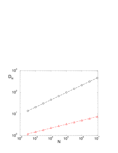
Figure 3: The average number of distinct degrees $D_{N}$ versus $N$ for networks that are grown by redirection with redirection probability $r$. The upper curve ($\circ$) corresponds to $A_{k}=k-\frac{1}{2}$ or to redirection probability $r=\frac{2}{3}$. Here the degree distribution exponent is 5/2 and $D_{N}=BN^{2/5}$, with $B=(3/2)^{2/5}\pi^{-1/5}\Gamma(3/5)=1.393019\ldots$. The lower curve ($\bigtriangleup$) corresponds to $A_{k}=k$ or $r=\frac{1}{2}$. Here $D_{N}$ is given by (5). Each data point represents an average over $10^{4}$ realizations. The dashed lines correspond to the theoretical prediction (1).

To determine the number of distinct degrees that appear in a typical realization of a large network, first notice that for $k$ in the range $k\leq K=(NR)^{1/\nu}$, $N_{k}\geq 1$. In this dense regime of the degree distribution (Fig. 2), all degrees with $k<K$ are present. This range therefore gives a contribution of $(NR)^{1/\nu}$ to $D_{N}$. In the complementary sparse range of $k>K$, we estimate the number of distinct degrees, by integrating the degree distribution for $k>K$. Adding the contributions from the dense and sparse regimes gives

$$D_{N}^{\text{naive}}=\frac{\nu}{\nu-1}\,K,\qquad\qquad K=(NR)^{1/\nu}\,.$$ (3)

While the $N$-dependence is correct, $D_{N}\sim N^{1/\nu}$, the amplitude is wrong. A better estimate can be obtained by assuming that the probability distribution for the number of nodes of each degree $k$ is the Poisson distribution with average value $N_{k}$ given by (2). Then $P_{k}\equiv\,\mathrm{Prob[(\#\ nodes\ of\ degree\ }k)\geq 1]=1-\exp(-N_{k})$. Using this property leads to a more accurate estimate (this same approach was developed in Ref. [13])

$$D_{N}=\sum_{k\geq 1}\left[1-e^{-N_{k}}\right]\,.$$ (4)

Replacing the sum by an integral, we ultimately obtain (1). For strictly linear preferential attachment, $R=4$ and $\nu=3$, so that

$$D_{N}=BN^{1/3}\qquad B=2^{2/3}\Gamma\left(\tfrac{2}{3}\right)=2.149528\ldots$$ (5)

In contrast, the naive estimate (3) for the amplitude is $B_{\text{naive}}=3\cdot 2^{-1/3}=2.381101\ldots$, which exceeds the more accurate value by $\approx 11\%$.

Generally $D_{N}/D_{N}^{\text{naive}}=\Gamma\left(2-\tfrac{1}{\nu}\right)$, so for the admissible range of $2<\nu<\infty$, this ratio monotonically increases from $\tfrac{1}{2}\sqrt{\pi}\approx 0.886227$ to 1. As shown in Fig. 3, simulation results are in excellent agreement with our theoretical predictions. A more detailed asymptotic analysis (employing methods developed in Ref. [19]) indicates that the average number of distinct degrees admits the expansion, $D_{N}=BN^{1/3}+C+\ldots$ for strictly linear preferential attachment. This allows us to extract a precise estimate of $B$ from the data that is in excellent agreement with Eq. (5).

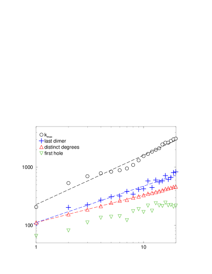
Figure 4: The maximum degree (number of citations) and the number of distinct degrees for the Physical Review citation network during the period 1893–2003. Also shown are the locations of the last dimer and the first hole. The dashed lines are the power-law fits with respective exponents 0.849. 0.627, 0.474,and 0.430. The data are measured at 20 equally-spaced network sizes as discussed in the text.

The general behavior outlined above for the number of distinct degrees and related quantities is also observed in the citation network of the Physical Review. Because this journal has grown roughly exponentially with time [20, 21], it is not appropriate to use publication date as a proxy for the network size. Since the citation data is presented as a list of links, each in the form of citing paper $\to$ cited paper, it is more natural to use the chronologically-ordered number of links as the proxy for network size. We use the Physical Review citation data as of 2003, which contains $L=3,110,866$ total links (citations). The maximum network degree (the highest-cited paper), the location of the last dimer, the number of distinct degrees, and the location of the first hole dimer are measured when the network size is $\frac{m}{20}L$, with $m=1,2,\ldots,20$ (Fig. 4).

Naive power-law fits to the first three datasets in Fig. 4 give $k_{\rm max}\sim L^{0.849}$, $D_{L}\sim L^{0.627}$, and $\langle h_{1}\rangle\sim L^{0.474}$. Let us provisionally assume that the citation distribution has a power-law dependence on $L$ and, by implication, the same dependence on $N$. Using $k_{\rm max}\sim N^{1/(\nu-1)}$ and the dependences for the number of distinct degrees and location of the last dimer given in Eqs. (3) and (LABEL:V), we infer the respective exponents for the degree-distribution exponent values of 2.18, 2.09, and 2.11. Thus these three properties are internally consistent under the assumption the citation distribution has a power-law form with exponent in the range $2.1$–$2.2$.

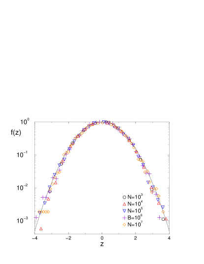
Figure 5: Scaled distribution of distinct degrees $f(z)$ for $N$ up to $10^{7}$, with $10^{4}$ network realizations for each $N$, for redirection probability $\frac{1}{2}$ (corresponding to strictly linear preferential attachment). The smooth curve is a Gaussian fit to the data. Visually identical data occurs for other redirection probabilities.

Our simulation results indicate that the random quantity $D_{N}$ is self-averaging. For strictly linear preferential attachment, we find that the standard deviation grows as $\sqrt{\langle D_{N}^{2}\rangle-\langle D_{N}\rangle^{2}}\sim N^{1/6}$. Moreover, the probability distribution $\Pi(D_{N})$ of distinct degrees fits the Gaussian

$$\Pi(D_{N})=\frac{1}{\sqrt{2\pi\sigma^{2}}}\,\,e^{-(D_{N}-\langle D_{N}\rangle)^{2}/2\sigma^{2}}$$ (6)

extremely well (Fig. 5). In appropriately scaled coordinates, this form universally holds for any redirection probability (equivalently different $\lambda$ values in the attachment rate $A_{k}=k+\lambda$). Moreover, the scaled distributions $f(z)\equiv\sqrt{2\pi\sigma^{2}}\,\Pi(D_{N})$, with $z=\sqrt{(\langle D_{N}^{2}\rangle-\langle D_{N}\rangle^{2})/2\sigma^{2}}$, are virtually identical for different $\lambda$ values.

3 The First Hole

We now study properties of the degree distribution in the sparse regime, where not every degree is represented. First consider the location of the first “hole” in the degree distribution—the smallest degree value for which $N_{k}=0$. We define $h_{1}$ as the degree value of the first hole, $h_{2}$ as the degree of the second hole, etc.

To determine the location of the first hole, it is useful to use the probability $P(h)$ that there are no holes in the degree distribution within the range $[1,h]$. This coincides with the probability that there is at least one node of degree $k$ for every $k$ between 1 and $h$. Again under the assumption that the number of nodes of degree $k$ is given by an independent Poisson distribution for each $k$, this probability is given by

$$P(h)=\prod_{1\leq k\leq h}\left[1-e^{-N_{k}}\right]\,.$$ (7)

We estimate the location of the first hole from the criterion $P(h_{1})=\frac{1}{2}$; however, any constant between 0 and 1 could equally well be chosen in this condition. Taking the logarithm of (7) and using $\ln\left[1-e^{-N_{k}}\right]\approx-e^{-N_{k}}$ (which is justifiable since $e^{-N_{k}}\ll 1$ when $k\leq h_{1}$), gives the following for the average location $\langle h_{1}\rangle$ of the first hole:

$$\int_{1}^{\langle h_{1}\rangle}dk\,e^{-N_{k}}=\ln 2\,.$$ (8)

Using Eq. (2) in (8) we find

$$\langle h_{1}\rangle\simeq\left(\frac{\nu NR}{\ln H}\right)^{1/\nu},\qquad H\sim\frac{\nu NR}{[\ln(\nu NR)]^{1+\nu}}~{}.$$ (9a)

Since $$H H$$ appears inside the logarithm, one can ignore the logarithmic factor in itself, thereby giving the simpler and still asymptotically exact formula

$$\langle h_{1}\rangle\simeq\left(\frac{\nu NR}{\ln N}\right)^{1/\nu}~{}.$$ (9b)

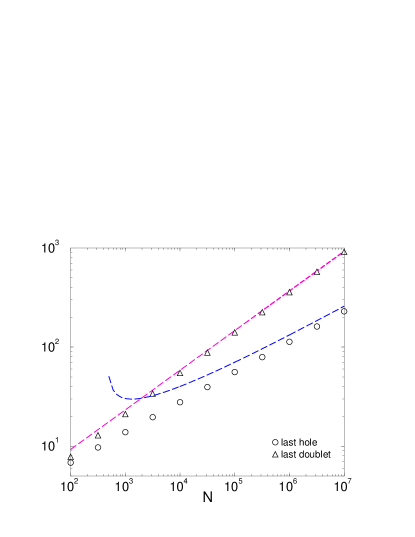
Figure 6: Location of the last hole and the last doublet as a function of $N$ for $10^{4}$ realizations of networks that are grown by strictly linear preferential attachment. The dashed curve is the prediction (9a), while the straight dashed line is the prediction from Eq. (LABEL:V).

It is worth noting that the naive calculation that leads to (3) for the number of distinct degrees ignores the possibility that holes exist in the range $k\leq(NR)^{1/\nu}$. According to Eq. (9b), however, the first hole appears earlier than $(NR)^{1/\nu}$ in the $N\to\infty$ limit. For a terrestrial-scale network with, say $N=10^{9}$ nodes, the location of the first hole will be roughly 3 times smaller than that predicted by the naive estimate (3).

4 Last Doublet and Last Dimer

Somewhere in the tail of the degree distribution lies the last doublet, the largest two consecutive $k$ values for which $N_{k}>0$, and the last dimer, the largest $k$ value for which $N_{k}=2$ (Fig. 2). Starting with degree 1, the degree distribution first consists of a long string of consecutive “occupied” degrees $1\leq k<h_{1}$, followed by a second string in the degree range $h_{1}<k<h_{2}$, etc. As the degree increases, these strings become progressively shorter and above a certain threshold all remaining strings are singlets. For a large network, the last string that is not a singlet will almost certainly be a doublet (with probability approaching 1 as $N\to\infty$). We now determine the average position of this last doublet.

The probability to have a doublet at $(k,k+1)$ is $N_{k}^{2}$ when $k\gg K=(NR)^{1/\nu}$. To estimate the position of the last doublet $(\delta,\delta+1)$ we employ the extremal criterion

$$\sum_{k\geq\delta}N_{k}^{2}\sim 1$$ (10)

that there should be of the order of one doublet in the degree range $(\delta,\infty)$. Using $N_{k}\sim NR\,k^{-\nu}$, we obtain

$$\langle\delta\rangle=C(RN)^{1/(\nu-1/2)}\,,$$ (11a)

with $$C$$ a constant, for the average position of the last doublet. Notice that the position of the last doublet also coincides, up to a prefactor of the order of 1, to the position of the last dimer. A more precise approach to determine the average location of the last doublet gives the amplitude as

$$C=(2\nu-1)^{-1/(2\nu-1)}\Gamma\!\left(\frac{2\nu-2}{2\nu-1}\right)~{}.$$ (11b)

To establish (11b), we use the the independent Poisson approximation to write, for the probability $F(\delta)$ to have no doublets in the degree range $k>\delta$,

$$F(\delta)=\prod_{k>\delta}\left[1-\left(1-e^{-N_{k}}\right)^{2}\right]\,.$$ (12)

This expression is the straightforward generalization of Eq. (7) to the case of dimers. Since the average number of nodes with degrees in the range $k>\delta$ is small, the product on the right-hand side of (12) simplifies to $\exp\!\left[-\int_{\delta}^{\infty}dk\,N_{k}^{2}\right]$. Computing the integral gives

$$F=\exp[-(\delta_{0}/\delta)^{2\nu-1}],\qquad\qquad\delta_{0}=\left(\frac{R^{2}N^{2}}{2\nu\!-\!1}\right)^{1/(2\nu\!-\!1)}.$$ (13)

The probability density $\Phi=\frac{dF}{d\delta}$ for the last doublet is then

$$\Phi(\delta)=\frac{2\nu-1}{\delta}\left(\frac{\delta_{0}}{\delta}\right)^{2\nu-1}\exp\!\left[-\left({\delta_{0}}{\delta}\right)^{2\nu-1}\right]\,,$$ (14)

from which the average position of the last doublet is given by

$$\langle\delta\rangle=\int_{0}^{\infty}d\delta\,\,\delta\,\Phi(\delta)=\int_{0}^{\infty}d\delta\,[1-F(\delta)]\,.$$ (15a)

Substituting (13) into (15a) leads to

$$\langle\delta\rangle=\Gamma\!\left(\frac{2\nu-2}{2\nu-1}\right)\delta_{0}\,.$$ (15b)

which reproduces (11). Similarly, the mean-square position of the last doublet is

$$\langle\delta^{2}\rangle=\int_{0}^{\infty}d\delta\,\,\delta^{2}\,\Phi(\delta)=2\int_{0}^{\infty}d\delta\,\delta\,[1-F(\delta)]\,,$$ (16)

from which the variance is

$$\langle\delta^{2}\rangle-\langle\delta\rangle^{2}=\left[\Gamma\!\left(\frac{2\nu-3}{2\nu-1}\right)-\Gamma^{2}\!\left(\frac{2\nu-2}{2\nu-1}\right)\right]\delta_{0}^{2}\,.$$ (17)

For strictly linear preferential attachment network growth, the above results reduce to

$$\begin{split}&\langle\delta\rangle=AN^{2/5},\qquad~{}~{}\,\,A=(\tfrac{16}{5})^{1/5}\Gamma(\tfrac{4}{5})=1.469158\ldots\\ &{\langle\delta^{2}\rangle^{1/2}}=V\langle\delta\rangle,\qquad\,V=\frac{\sqrt{\Gamma(3/5)}}{\Gamma(4/5)}=1.048182\ldots\end{split}$$ (18)

Following the same line of reasoning, the position of the last triplet, $(\tau-1,\tau,\tau+1)$, is given by

$$\langle\tau\rangle\sim N^{1/(\nu-1/3)}\,.$$ (19)

For strictly linear preferential attachment, this result gives the dependence $\langle\tau\rangle\sim N^{3/8}$. Our simulation data are consistent with the predictions (LABEL:V)–(19) (Fig. 6).

5 Discussion

For any broadly distributed integer-valued variable, the underlying distribution exhibits intriguing features that stem from the combined influences of discreteness and finiteness. Such a distribution is smooth in a dense regime, where every integer value of the variable has a non-zero probability of occurrence. In the complementary sparse regime, a variety of statistical anomalies arise that quantify the extent of the sparseness (Fig. 2).

For the degree distribution of complex networks that genererically have power-law tails, $N_{k}\sim N/k^{\nu}$, our main results are: (i) The number of distinct degrees in a network of $N$ nodes scales as $N^{1/\nu}$. This generic behavior is also observed in the citation network of the Physical Review. (ii) The distribution in the number of distinct degrees is very well fit by a universal Gaussian function. (iii) There is a rich set of behaviors for basic characteristics of the sparse regime, such as the positions of holes (zeros) in the distribution, as well as the locations of doublet, triplets, etc., and the locations of dimers, trimers, etc. All of these quantities can be determined by simple probabilistic reasoning.

Our analysis tacitly assumed that the number of nodes of different degrees, $N_{i}$ and $N_{j}$ for $i\neq j$, are uncorrelated, and that the $N_{k}$’s are Poisson distributed random quantities. While these assumptions are questionable in the sparse regime, predictions that are based on these assumptions are in excellent agreement with results from simulations of preferential attachment networks. While we believe that our predictions are asymptotically exact, a more rigorous analysis is needed to justify them and explain their validity (or at least their impressive accuracy). A challenging extension of this work is to probe the fluctuations in the total number of distinct degrees. The mechanism for the observed Gaussian shape of the distribution of distinct degrees is not at all evident. In fact, for networks that grow by redirection, with redirection becoming more certain as the degree of the ancestor node increases, the total number of distinct degrees is not even a self-averaging quantity [26].

Our methods apply equally well to other heavy-tailed integer-valued distributions, such as the cluster-size distribution in classical percolation [27] and in protein interaction and regulatory networks [28]. The latter models often exhibit an infinite-order percolation transition, in which the cluster-size distribution has an algebraic tail in the entire non-percolating phase [29, 30, 31, 32, 33, 34, 35, 36]. Our approach leads to new results for the total number of distinct cluster types $C_{N}$, for the position of the first hole (the minimal size that is not present), etc.

For concreteness, consider networks that are built by adding nodes one at a time with each new node connecting to $k$ randomly chosen existing nodes with probability $p_{k}$ [35, 36]. While the set of probabilities $p_{k},k=0,1,2,\ldots$, with $\sum_{k\geq 0}p_{k}=1$, fully defines the network ensemble, only the first two moments, $\langle k\rangle=\sum_{k\geq 1}kp_{k}$ and $\Delta=\langle k^{2}\rangle-\langle k\rangle^{2}$, matter in determining large-scale properties. In the non-percolating phase, $\langle k\rangle<\frac{1}{2}$ and $\Delta<\frac{1}{4}$, we use the decay exponent for the cluster-size distribution that was determined in [36] to obtain

$$C_{N}\sim N^{\delta},\qquad\qquad\delta=\frac{1-\sqrt{1-4\Delta}}{3-\sqrt{1-4\Delta}}~{}.$$

At the percolation transition, $\langle k\rangle<\frac{1}{2}$ and $\Delta=\frac{1}{4}$, the tail of the cluster-size distribution contains universal (independent of $\langle k\rangle$ and $\Delta$) algebraic and logarithmic factors, viz. $c_{s}\simeq 2(1-2\langle k\rangle)^{-2}s^{-3}(\ln s)^{-2}$ for $s\gg 1$. A straightforward generalization of our previous analysis shows that the total number of distinct cluster types grows as

$$C_{N}\simeq 2^{1/3}\,\Gamma\big{(}\tfrac{2}{3}\big{)}\,\Big{(}\frac{3}{1-2\langle k\rangle}\Big{)}^{2/3}\left[\frac{N}{(\ln N)^{2}}\right]^{1/3}.$$

As a final note, this work has focused broadly on properties associated with the support of discrete distribution. The averages of these properties over a large ensemble of networks have systematic dependences on the number of nodes $N$ in the network; however, the behavior in each network realization may not be monotonic. Thus while $k_{\rm max}$ is clearly a non-decreasing function of $N$, the number of distinct degrees and the locations of quantities like the first hole or the last doublet can both increase or decrease with $N$. This intriguing aspect of the problem may provide a more detailed understanding of how a complex network actually grows.

We gratefully acknowledge partial financial support from AFOSR and DARPA grant #FA9550-12-1-0391, and from NSF grant No. DMR-1205797. We also thank A. Gabel for collaborations at a preliminary stage of this project. Finally, we thank the American Physical Society editorial office for providing the citation data.

References

- [1] M. E. J. Newman, Networks: An Introduction (Oxford Univ. Press, Oxford, 2010).
- [2] R. Albert and A.-L. Barabási, Rev. Mod. Phys. 74, 47 (2002).
- [3] G. U. Yule, Phil. Trans. Roy. Soc. B 213, 21 (1925).
- [4] H. A. Simon, Biometrica 42, 425 (1955).
- [5] D. J. de Solla Price, Science 149, 510 (1965); J. Amer. Soc. Inform. Sci. 27, 292 (1976).
- [6] A. L. Barabási and R. Albert, Science 286, 509 (1999).
- [7] P. L. Krapivsky, S. Redner, and F. Leyvraz, Phys. Rev. Lett. 85, 4629 (2000).
- [8] S. N. Dorogovtsev, J. F. F. Mendes, and A. N. Samukhin, Phys. Rev. Lett. 85, 4633 (2000).
- [9] G. Herdan, Type-Token Mathematics (Mouton, The Hague, 1960).
- [10] H. S. Heaps, Information Retrieval: Computational and Theoretical Aspects (Academic Press, New York, 1978)
- [11] D. D. van Leijenhorst and T. P. van der Weide, Infor. Sci. 170, 263 (2005).
- [12] L. Lu, Z.-K. Zhang, and T. Zhou, PLoS ONE 5, e14139 (2010).
- [13] M. Gerlach and E. G. Altmann, arXiv:1212.1362.
- [14] G. K. Zipf, The Psychobiology of Language (Routledge, London, 1936).
- [15] P. Erdős and T. Gallai, Matematikai Lapok 11, 264 (1960).
- [16] C. I. Del Genio, H. Kim, Z. Toroczkai, and K. E. Bassler, PLoS ONE 5, e10012 (2010).
- [17] C. I. Del Genio, T. Gross, and K. E. Bassler, Phys. Rev. Lett. 107, 178701 (2011).
- [18] P. L. Krapivsky and S. Redner, Phys. Rev. E 63, 066123 (2001).
- [19] P. L. Krapivsky and S. Redner, J. Phys. A 35, 9517 (2002).
- [20] S. Redner, Physics Today 58, 49 (2005); S. Redner, arXiv:physics/0407137.
- [21] P. L. Krapivsky and S. Redner, Phys. Rev. E 71, 036118 (2005).
- [22] M. L. Wallace, V. Lariviere, and Y. Gingras, J. Informetrics 3, 296 (2009).
- [23] J. C. Phillips, arxiv:0909.5363.
- [24] G. J. Peterson, S. Presse, and K. A. Dill, Proc. Natl. Acad. Sci. (USA) 107 16023 (2010).
- [25] M. Golosovsky and S. Solomon, Phys. Rev. Lett. 109, 098701 (2012); M. Golosovsky and S. Solomon, Eur. Phys. J. Special Topics 205, 303 (2012).
- [26] A. Gabel, P. L. Krapivsky, and S. Redner, in preparation.
- [27] D. Stauffer and A. Aharony, Introduction to Percolation Theory, 2nd ed. (Taylor and Francis, London, 1991).
- [28] P. L. Uetz et al., Nature (London) 403, 623 (2000); T. Ito et al., Proc. Natl. Acad. Sci. U.S.A. 97, 1143 (2000).
- [29] D. S. Callaway, J. E. Hopcroft, J. M. Kleinberg, M. E. J. Newman, and S. H. Strogatz, Phys. Rev. E 64, 041902 (2001).
- [30] S. N. Dorogovtsev, J. F. F. Mendes, and A. N. Samukhin, Phys. Rev. E 64, 066110 (2001).
- [31] P. L. Krapivsky and S. Redner, Computer Networks 39, 261 (2002).
- [32] J. Kim, P. L. Krapivsky, B. Kahng, and S. Redner, Phys. Rev. E 66, 055102 (2002).
- [33] D. Lancaster, J. Phys. A 35, 1179 (2002).
- [34] M. Bauer and D. Bernard, J. Stat. Phys. 111, 703 (2003).
- [35] C. Coulomb and M. Bauer, Eur. Phys. J. B. 35, 377 (2003).
- [36] P. L. Krapivsky and B. Derrida, Physica A 340, 714 (2004).