One-Bit Quantization Design and Adaptive Methods for Compressed Sensing

Abstract

There have been a number of studies on sparse signal recovery from one-bit quantized measurements. Nevertheless, little attention has been paid to the choice of the quantization thresholds and its impact on the signal recovery performance. This paper examines the problem of one-bit quantizer design for sparse signal recovery. Our analysis shows that the magnitude ambiguity that ever plagues conventional one-bit compressed sensing methods can be resolved, and an arbitrarily small reconstruction error can be achieved by setting the quantization thresholds close enough to the original unquantized measurements. Note that the unquantized data are inaccessible by us. To overcome this difficulty, we propose an adaptive quantization method that iteratively refines the quantization thresholds based on previous estimate of the sparse signal. Numerical results are provided to collaborate our theoretical results and to illustrate the effectiveness of the proposed algorithm.

I Introduction

Compressive sensing is a recently emerged paradigm of signal sampling and reconstruction, the main purpose of which is to recover sparse signals from much fewer linear measurements [1, 2]

$$\boldsymbol{y}=\boldsymbol{Ax}$$ (1)

where $\boldsymbol{A}\in\mathbb{R}^{m\times n}$ is the sampling matrix with $m\ll n$, and $\boldsymbol{x}$ denotes the $n$-dimensional sparse signal with only $K$ nonzero coefficients. Such a problem has been extensively studied and a variety of algorithms that provide consistent recovery performance guarantee were proposed, e.g. [1, 2, 3, 4]. Conventional compressed sensing assumes infinite precision of the acquired measurements. In practice, however, signals need to be quantized before further processing, that is, the real-valued measurements need to be mapped to discrete values over some finite range. Besides, in some sensing systems (e.g. distributed sensor networks), data acquisition is expensive due to limited bandwidth and energy constraints [5]. Aggressive quantization strategies which compress real-valued measurements into one or only a few bits of data are preferred in such scenarios. Another benefit brought by low-rate quantization is that it can significantly reduce the hardware complexity and cost of the analog-to-digital converter (ADC). As pointed out in [6], low-rate quantizer can operate at a much higher sampling rate than high-resolution quantizer. This merit may lead to a new data acquisition paradigm which reconstructs the sparse signal from over-sampled but low-resolution measurements.

Inspired by practical necessity and potential benefits, compressed sensing based on low-rate quantized measurements has attracted considerable attention recently, e.g. [7, 8, 9]. In particular, the problem of recovering a sparse or compressible signal from one-bit measurements

$$\boldsymbol{b}=\text{sign}(\boldsymbol{y})=\text{sign}(\boldsymbol{A}\boldsymbol{x})$$ (2)

was firstly introduced by Boufounos and Baraniuk in their work [10], where “sign” denotes an operator that performs the sign function element-wise on the vector, the sign function returns $1$ for positive numbers and $-1$ otherwise. Following [10], the reconstruction performance from one-bit measurements was more thoroughly studied and a variety of one-bit compressed sensing algorithms such as binary iterative hard thresholding (BIHT) [11], matching sign pursuit (MSP) [12], and many others [13, 14, 15] were proposed. Despite all these efforts, very little is known about the optimal choice of the quantization thresholds and its impact on the recovery performance. In most previous work (e.g [10, 11, 12, 13, 6, 14, 15]), the quantization threshold is set equal to zero. Nevertheless, such a choice does not necessarily lead to the best reconstruction accuracy. In fact, in this case, only the sign of the measurement is retained while the information about the magnitude of the signal is lost. Hence an exact reconstruction of the sparse signal is impossible without additional information regarding the sparse signal. In some other scenarios such as intensity-based source localization in sensor networks, since all sampled measurements are non-negative, comparing the original measurements with zero yields all ones wherever the sources are located, which makes identifying the true locations impossible. From the above discussions, we can see that quantization is an integral part of the sparse signal recovery and is critical to the recovery performance.

There have been some interesting work [16, 17, 18] on quantizer design for compressed sensing. Specifically, the work [16] utilizes the high-resolution distributed functional scalar quantization theory for quantizer design, where the quantization error is modeled as random noise following a certain distribution. Nevertheless, such modeling holds valid only for high-resolution quantization, and may bring limited benefits when a low-rate quantization strategy is adopted. In [17, 18], authors proposed a generalized approximate message passing (GAMP) algorithm for quantized compressed sensing, and studied the quantizer design under the GAMP reconstruction. The method [17, 18] was developed in a Bayesian framework by modeling the sparse signal as a random variable and minimizing the average reconstruction error with respective to all possible realizations of the sparse signal. This method, however, involves high-dimensional integral or multidimensional search to find the optimal quantizer, which makes a close-form expression of the optimal quantizer design difficult to obtain. In [18], an adaptive algorithm was proposed which adjusts the thresholds such that the hyperplanes pass through the center of the mass of the probability distribution of the estimated signal. Albeit intuitive, no rigorous theoretical guarantee was available to justify the proposed adaptive method. The problem of reconstructing image from one-bit quantized data is considered in [19], where the quantization thresholds are set such that the binary measurements are acquired with equal probability. Such a scheme has been shown to be empirically effective. Nevertheless, it is still unclear why it leads to better reconstruction performance.

In this paper, we investigate the problem of one-bit quantization design for recovery of sparse signals. The study is conducted in a deterministic framework by treating the sparse signal as a deterministic parameter. We provide an quantitative analysis which examines the choice of the quantization thresholds and quantifies its impact on the reconstruction performance. Analyses also reveal that the reconstruction error can be made arbitrarily small by setting the quantization thresholds close enough to the original unquantized measurements $\boldsymbol{y}$. Since the original unquantized data samples $\boldsymbol{y}$ are inaccessible by us, to address this issue, we propose an adaptive quantization approach which iteratively adjusts the quantization thresholds such that the thresholds eventually come close to the original data samples and thus a small reconstruction error is achieved.

The rest of the paper is organized as follows. In Section II, we introduce the one-bit compressed sensing problem. The main results of this paper are presented in Section III, where we show that, by properly selecting the quantization thresholds, sparse signals can be recovered from one-bit measurements with an arbitrarily small error. A rigorous proof of our main result is provided in Section IV. An adaptive quantization method is developed in V to iteratively refine the thresholds based on previous estimate. In Section VI, numerical results are presented to corroborate our theoretical analysis and illustrate the effectiveness of the proposed algorithm, followed by concluding remarks in Section VII.

II Problem Formulation

We consider a coarse quantization-based signal acquisition model in which each real-valued sample is encoded into one-bit of information

$$\boldsymbol{b}=\text{sign}(\boldsymbol{y}-\boldsymbol{\tau})=\text{sign}(\boldsymbol{A}\boldsymbol{x}-\boldsymbol{\tau})$$ (3)

where $\boldsymbol{b}=[b_{1}\phantom{0}b_{2}\phantom{0}\ldots\phantom{0}b_{m}]^{T}$ are the binary observations, and $\boldsymbol{\tau}=[\tau_{1}\phantom{0}\tau_{2}\phantom{0}\ldots\phantom{0}\tau_{m}]^{T}$ denotes the quantization threshold vector. As mentioned earlier, in most previous one-bit compressed sensing studies, the quantization thresholds are set equal to zero, i.e. $\boldsymbol{\tau}=\boldsymbol{0}$. A major issue with the zero quantization threshold is that it introduces a magnitude ambiguity which cannot be resolved without additional information regarding the sparse signal. The reason is that when $\boldsymbol{\tau}=\boldsymbol{0}$, multiplying $\boldsymbol{x}$ by any arbitrary nonzero scaling factor will result in the same quantized data $\{b_{n}\}$. To circumvent the magnitude ambiguity issue, in [11, 13], a unit-norm constraint is imposed on the sparse signal and it was shown that unit-norm signals can be recovered with a bounded error from one bit quantized data. Nevertheless, the choice of the zero threshold is not necessarily the best. In this paper, we are interested in examining the choice of the quantization thresholds and its impact on the reconstruction performance.

Specifically, we consider the following canonical form for sparse signal reconstruction

$$\min_{\boldsymbol{z}}\|\boldsymbol{z}\|_{0}\quad\text{s.t.}\phantom{0}\text{sign}(\boldsymbol{A}\boldsymbol{z}-\boldsymbol{\tau})=\boldsymbol{b}$$ (4)

Such an optimization problem, albeit non-convex, is more amenable for theoretical analysis than its convex counterpart (43). Suppose $\boldsymbol{\hat{x}}$ is a solution of the above optimization. In the following, we examine the choice of $\boldsymbol{\tau}$ and its impact on the reconstruction error $\|\boldsymbol{x}-\boldsymbol{\hat{x}}\|_{2}$.

III One-Bit Quantization Design: Analysis

To facilitate our analysis, we decompose the quantization threshold vector $\boldsymbol{\tau}$ into a sum of two terms:

$$\boldsymbol{\tau}=\boldsymbol{y}-\boldsymbol{\delta}$$ (5)

where $\boldsymbol{\delta}=[\delta_{1}\phantom{0}\delta_{2}\phantom{0}\ldots\phantom{0}\delta_{m}]^{T}$ can be treated as a constrained deviation from the original unquantized measurements $\boldsymbol{y}$. Substituting (5) into (3), we get

$$\boldsymbol{b}=\text{sign}(\boldsymbol{A}\boldsymbol{x}-\boldsymbol{\tau})=\text{sign}(\boldsymbol{\delta})$$ (6)

Suppose $\hat{\boldsymbol{x}}$ is the solution of (4). Let $\boldsymbol{h}\triangleq\hat{\boldsymbol{x}}-\boldsymbol{x}$ be the residual (reconstruction error) vector. Clearly, $\boldsymbol{h}$ is a $2K$-sparse vector which has at most $2K$ nonzero entries since $\hat{\boldsymbol{x}}$ has at most $K$ nonzero coefficients. Also, the solution $\hat{\boldsymbol{x}}$ yields estimated measurements that are consistent with the observed binary data, i.e.

$$\boldsymbol{b}=\text{sign}(\boldsymbol{A}\boldsymbol{\hat{x}}-\boldsymbol{\tau})=\text{sign}(\boldsymbol{Ah}+\boldsymbol{\delta})$$ (7)

Combining (6) and (7), the residual vector $\boldsymbol{h}$ has to satisfy the following constraint

$$\text{sign}(\boldsymbol{Ah}+\boldsymbol{\delta})=\text{sign}(\boldsymbol{\delta})$$ (8)

In the following, we will show that the residual vector $\boldsymbol{h}$ can be bounded by the deviation vector $\boldsymbol{\delta}$ if the number of measurements are sufficiently large and $\boldsymbol{A}$ satisfies a certain condition. Thus the reconstruction error $\boldsymbol{h}$ can be made arbitrarily small by setting $\boldsymbol{\delta}$ close to zero. Our main results are summarized as follows.

Theorem 1

Let $\boldsymbol{x}\in\mathbb{R}^{n}$ be an $K$-sparse vector. $\boldsymbol{A}\in\mathbb{R}^{m\times n}$ is the sampling matrix. Suppose there exist an integer $\kappa\geq 2K$ and a positive parameter $\mu$ such that any $\kappa\times n$ submatrix $\boldsymbol{\bar{A}}$ constructed by selecting certain rows of $\boldsymbol{A}$ satisfies

$$\|\boldsymbol{\bar{A}}\boldsymbol{u}\|_{2}^{2}\geq\mu\|\boldsymbol{u}\|_{2}^{2}$$ (9)

for all $2K$-sparse vector $\boldsymbol{u}$. Also, assume that each entry of $\boldsymbol{\delta}$ is independently generated from a certain distribution with equal probabilities being positive or negative. Let $\boldsymbol{\hat{x}}$ denote the solution of the optimization problem (4). For any arbitrarily small value $\eta>0$, we can ensure that the following statement is true with probability exceeding $1-\eta$: if the number of measurements, $m$, is sufficiently large and satisfies

$$m-2K\log(m-\kappa+1)-(\kappa-1)\log m$$

$$\geq 2K(\log(ne^{2})-2\log(2K)+1)+\log(1/\eta)+c$$ (10)

then the sparse signal can be recovered from (4) with the reconstruction error bounded by

$$\|\boldsymbol{\hat{x}}-\boldsymbol{x}\|_{2}\leq\frac{\epsilon}{\sqrt{\mu}}\triangleq\lambda\epsilon$$ (11)

where $\epsilon\triangleq\|\boldsymbol{\delta}\|_{2}$, $\lambda\triangleq 1/\sqrt{\mu}$, $e$ in (10) represents the base of the natural logarithm, and $c$ in (10) is defined as

$$c\triangleq(\kappa-1)(\log(e/(\kappa-1))+1)$$ (12)

which is a constant only dependent on $\kappa$.

We have the following remarks regarding Theorem 1.

Remark 1: Clearly, the condition (9) is guaranteed if there exists a constant $\gamma_{2K}<1$ such that any $\kappa\times n$ submatrix of $\boldsymbol{A}$ satisfies

$$(1+\gamma_{2K})\|\boldsymbol{u}\|_{2}^{2}\geq\|\boldsymbol{\bar{A}u}\|_{2}^{2}\geq(1-\gamma_{2K})\|\boldsymbol{u}\|_{2}^{2}$$ (13)

for all $2K$-sparse vector $\boldsymbol{u}$. As indicated in previous studies [1], when the sampling matrix is randomly generated from a Gaussian or Bernoulli distribution, this restricted isometry property is met with an overwhelming probability, particularly when $\kappa$ is large. Hence it is not difficult to find an integer $\kappa$ and a positive $\mu$ such that the condition (9) holds.

Remark 2: Note that the term on the left hand side of (10) is a monotonically increasing function of $m$ when $m$ is greater than a certain value. Thus for fixed values of $K$, $\kappa$, $n$, and $\eta$, we can always find a sufficiently large $m$ to ensure the condition (10) is guaranteed. In addition, a close inspection of (10) reveals that, for a constant $\eta$, the number of measurements required to guarantee (10) is of order $\mathcal{O}(K\log(n))$, which is the same as that for conventional compressed sensing.

Remark 3: From (11), we see that the sparse signal can be recovered with an arbitrarily small error by letting $\boldsymbol{\delta}\rightarrow\boldsymbol{0}$, or in other words, by setting the threshold vector $\boldsymbol{\tau}$ sufficiently close to the unquantized data $\boldsymbol{y}$. This result has two important implications. Firstly, sparse signals can be reconstructed with negligible errors even from one-bit measurements. We note that [11, 13] also showed that sparse signals can be recovered with a bounded error from one bit quantized data. But their analysis ignores the magnitude ambiguity and confines sparse signals on the unit Euclidean sphere. Such a sphere constraint is no longer necessary for our analysis. Secondly, our result suggests that the best thresholds should be set as close to the original data samples $\boldsymbol{y}$ as possible. So far there has no theoretical guarantee indicating that other choice of thresholds can also lead to a stable recovery with an arbitrarily small reconstruction error.

IV Proof of Theorem 1

Let $\boldsymbol{a}_{i}^{T}$ denote the $i$th row of the sampling matrix $\boldsymbol{A}$. Clearly, to ensure the sign consistency (8) for each component, we should either have

$$\text{sign}(\boldsymbol{a}_{i}^{T}\boldsymbol{h})=\text{sign}(\delta_{i})$$ (14)

or

$$|\boldsymbol{a}_{i}^{T}\boldsymbol{h}|<|\delta_{i}|$$ (15)

Note that in the latter case the sign of $(\boldsymbol{a}_{i}^{T}\boldsymbol{h}+\delta_{i})$ does not flip regardless of the sign of $\boldsymbol{a}_{i}^{T}\boldsymbol{h}$. Therefore if there exists a $2K$-sparse residual vector $\boldsymbol{h}$ such that each component of $\boldsymbol{Ah}$ satisfies either (14) or (15), then $\boldsymbol{\hat{x}}=\boldsymbol{x}+\boldsymbol{h}$ is the solution of (4). Our objective in the following is to show that such a residual vector $\boldsymbol{h}$ is bounded by the deviation vector $\boldsymbol{\delta}$ with an arbitrarily high probability.

Without loss of generality, we decompose $\boldsymbol{A}$ and $\boldsymbol{\delta}$ into two parts: $\boldsymbol{A}=[\boldsymbol{A}_{1}^{T}\phantom{0}\boldsymbol{A}_{2}^{T}]^{T}$, $\boldsymbol{\delta}=[\boldsymbol{\delta}_{1}^{T}\phantom{0}\boldsymbol{\delta}_{2}^{T}]^{T}$, according to the two possible relationships between $\boldsymbol{a}_{i}^{T}\boldsymbol{h}$ and $\delta_{i}$:

$$\left.\begin{array}[]{cc}\text{sign}(\boldsymbol{A}_{1}\boldsymbol{h})=\text{sign}(\boldsymbol{\delta}_{1})\\ |\boldsymbol{A}_{2}\boldsymbol{h}|<|\boldsymbol{\delta}_{2}|\end{array}\right.$$ (18)

where $\boldsymbol{A}_{1}\in\mathbb{R}^{m_{1}\times n}$, $\boldsymbol{A}_{2}\in\mathbb{R}^{m_{2}\times n}$, $m_{1}+m_{2}=m$, and in the second equation, both the absolute value operation $|\cdot|$ and the inequality symbol “$<$” applies entrywise to vectors.

We now analyze the probability of the residual vector $\boldsymbol{h}$ being greater than $\lambda\epsilon$, given that the condition (18) is satisfied. This conditional probability can be denoted as $P(\|\boldsymbol{h}\|_{2}>\lambda\epsilon|\text{E})$, where we use “E” to denote the event (18). Clearly, $P(\|\boldsymbol{h}\|_{2}>\lambda\epsilon|\text{E})$ can also be explained as the probability that the event $\|\boldsymbol{h}\|_{2}>\lambda\epsilon$ will occur, when the event E has occurred. To facilitate our analysis, we divide the event (18) into two disjoint sub-events which are defined as

E1: The event (18) holds true for $$m_{2}\geq\kappa$$

E2: The event (18) holds true for $$m_{2}<\kappa$$

Clearly, the union of these two sub-events is equal to the event (18). Utilizing Bayes’ Theorem, the probability $P(\|\boldsymbol{h}\|_{2}>\lambda\epsilon|\text{E})$ can be expressed as

$$P(\|\boldsymbol{h}\|_{2}>\lambda\epsilon|\text{E})\stackrel{{\scriptstyle(a)}}{{=}} P(\|\boldsymbol{h}\|_{2}>\lambda\epsilon,\text{E})$$

$$= P(\|\boldsymbol{h}\|_{2}>\lambda\epsilon,\text{E1}\cup\text{E2})$$

$$\stackrel{{\scriptstyle(b)}}{{=}} P(\|\boldsymbol{h}\|_{2}>\lambda\epsilon,\text{E1})+P(\|\boldsymbol{h}\|_{2}>\lambda\epsilon,\text{E2})$$ (19)

where $(a)$ holds because the events (18) is a prerequisite condition that is always met to ensure the sign consistency, i.e. $P(\text{E})=1$, and $(b)$ follows from the fact that the probability of the union of two disjoint events is equal to the sum of their respective probabilities.

Let us first examine the probability $P(\|\boldsymbol{h}\|_{2}>\lambda\epsilon,\text{E1})$. We show that the events $\|\boldsymbol{h}\|_{2}>\lambda\epsilon$ and E1 are two mutually exclusive events which cannot occur at the same time. To see this, note that when the event E1 occurs, we should have

$$|\boldsymbol{A}_{2}\boldsymbol{h}|<|\boldsymbol{\delta}_{2}|\Rightarrow\|\boldsymbol{A}_{2}\boldsymbol{h}\|_{2}^{2}<\epsilon^{2}$$ (20)

in which $\boldsymbol{A}_{2}\in\mathbb{R}^{m_{2}\times n}$ and $m_{2}\geq\kappa$. On the other hand, recalling that any $\kappa\times n$ sub-matrix formed by selecting certain rows of $\boldsymbol{A}$ satisfies the condition (9), we have

$$\|\boldsymbol{A}_{2}\boldsymbol{h}\|_{2}^{2}\geq\mu\|\boldsymbol{h}\|_{2}^{2}$$ (21)

Combining (20) and (21), we arrive at

$$\|\boldsymbol{h}\|_{2}<\frac{\epsilon}{\sqrt{\mu}}\triangleq\lambda\epsilon$$ (22)

which is contradictory to the event $\|\boldsymbol{h}\|_{2}>\lambda\epsilon$. Hence the events E1 and $\|\boldsymbol{h}\|_{2}>\lambda\epsilon$ cannot occur simultaneously, which implies

$$P(\|\boldsymbol{h}\|_{2}>\lambda\epsilon,\text{E1})=0$$ (23)

Substituting (23) into (19), the probability $P(\|\boldsymbol{h}\|_{2}>\lambda\epsilon|\text{E})$ is simplified as

$$P(\|\boldsymbol{h}\|_{2}>\lambda\epsilon|\text{E})=P(\|\boldsymbol{h}\|_{2}>\lambda\epsilon,\text{E2})$$ (24)

The probability $P(\|\boldsymbol{h}\|_{2}>\lambda\epsilon,\text{E2})$, however, is still difficult to analyze. To circumvent this difficulty, we, instead, derive an upper bound on $P(\|\boldsymbol{h}\|_{2}>\lambda\epsilon,\text{E2})$:

$$P(\|\boldsymbol{h}\|_{2}>\lambda\epsilon,\text{E2})$$

$$= P(\|\boldsymbol{h}\|_{2}>\lambda\epsilon|\text{E2})P(\text{E2})\leq P(\text{E2})$$

$$\stackrel{{\scriptstyle(a)}}{{=}} P(\text{sign}(\boldsymbol{A}_{1}\boldsymbol{h})=\text{sign}(\boldsymbol{\delta}_{1}),|\boldsymbol{A}_{2}\boldsymbol{h}|<|\boldsymbol{\delta}_{2}|,m_{2}<\kappa)$$

$$\leq P(\text{sign}(\boldsymbol{A}_{1}\boldsymbol{h})=\text{sign}(\boldsymbol{\delta}_{1}),m_{2}<\kappa)$$

$$= P(\text{sign}(\boldsymbol{A}_{1}\boldsymbol{h})=\text{sign}(\boldsymbol{\delta}_{1}),m_{1}>m-\kappa)$$

$$\stackrel{{\scriptstyle(b)}}{{=}} P\bigg{(}\bigcup_{i=0}^{\kappa-1}\Omega_{i}\bigg{)}$$ (25)

where $(a)$ comes from the definition of the event E2, and in $(b)$, the event $\Omega_{i}$ is defined as

$$\Omega_{i}:\phantom{0} \text{sign}(\boldsymbol{A}_{1}\boldsymbol{h})=\text{sign}(\boldsymbol{\delta}_{1})$$

where $$\boldsymbol{A}_{1}\in\mathbb{R}^{m_{1}\times n} m_{1}=m-i$$, and (26)

which means that there exist at least $m-i$ components in $\boldsymbol{Ah}$ whose signs are consistent with the corresponding entries in $\boldsymbol{\delta}$. Note that since the rest $i$ components are not explicitly specified in $\Omega_{i}$, the event $\Omega_{i}$ include all possibilities for the rest $i$ components. Based on the definition of $\Omega_{i}$, we can infer the following relationship: $\Omega_{i_{1}}\supset\Omega_{i_{2}}$ for $i_{1}>i_{2}$. This is because $\Omega_{i_{2}}$ can be regarded as a special case of the event $\Omega_{i_{1}}$ with some of the unspecified $i_{1}$ components also meeting the sign consistency requirement. With this relation, the upper bound derived in (25) can be simplified as

$$P(\|\boldsymbol{h}\|_{2}>\lambda\epsilon,\text{E2})\leq P\bigg{(}\bigcup_{i=0}^{\kappa-1}\Omega_{i}\bigg{)}=P(\Omega_{\kappa-1})$$ (27)

We note that for the event $\Omega_{\kappa-1}$, $\boldsymbol{A}_{1}$ is not specified and can be any submatrix of $\boldsymbol{A}$. Considering selection of $m-\kappa+1$ rows (out of $m$ rows of $\boldsymbol{A}$) to construct $\boldsymbol{A}_{1}$, the event $\Omega_{\kappa-1}$ can be expressed as a union of a set of sub-events

$$\Omega_{\kappa-1}=\bigcup_{j=1}^{J}\Omega_{\kappa-1}^{j}$$ (28)

where $J\triangleq C(m,m-\kappa+1)$, $C(m,k)$ denotes the number of $k$ combinations from a given set of $m$-elements, and each sub-event $\Omega_{\kappa-1}^{j}$ is defined as

$$\Omega_{\kappa-1}^{j}:\text{sign}(\boldsymbol{A}_{1}\boldsymbol{h})=\text{sign}(\boldsymbol{\delta}_{1})\phantom{0}\text{where $\boldsymbol{A}_{1}=\boldsymbol{A}[I_{j},:]$}$$ (29)

in which $I_{j}$ is an unique index set which consists of $m-\kappa+1$ non-identical indices selected from $\{1,2,\ldots,m\}$, $\boldsymbol{A}[I_{j},:]$ denotes a submatrix of $\boldsymbol{A}$ constructed by certain rows from $\boldsymbol{A}$, and the indices of the selected rows are specified by $I_{j}$. From (28), we have

$$P(\Omega_{\kappa-1})= P\bigg{(}\bigcup_{j=1}^{J}\Omega_{\kappa-1}^{j}\bigg{)}\stackrel{{\scriptstyle(a)}}{{\leq}}\sum_{j=1}^{J}P(\Omega_{\kappa-1}^{j})$$ (30)

where the inequality $(a)$ follows from the fact that the probability of a union of events is no greater than the sum of probabilities of respective events. The inequality becomes an equality if the events are disjoint. Nevertheless, the sub-events $\{\Omega_{\kappa-1}^{j}\}$ are not necessarily disjoint and may have overlappings due to the $\kappa-1$ unspecified components.

We now analyze the probability $P(\Omega_{\kappa-1}^{j})$. To begin with our analysis, we introduce the concept of orthant originally proposed in [11] for analysis of one-bit compressed sensing. An orthant in $\mathbb{R}^{m}$ is a set of vectors that share the same sign pattern, i.e.

$$\mathcal{O}_{\tilde{\boldsymbol{u}}}=\{\boldsymbol{u}\in\mathbb{R}^{m}|\text{sign}(\boldsymbol{u})=\tilde{\boldsymbol{u}}\}$$ (31)

A useful result concerning intersections of orthants by subspaces is summarized as follows.

Lemma 1

Let $\mathcal{S}$ be an arbitrary $k$-dimensional subspace in an $m$-dimensional space. Then the number of orthants intersected by $\mathcal{S}$ can be upper bounded by

$$I(m,k)\leq 2^{k}C(m,k)$$ (32)

where $C(m,k)$ denotes the number of $k$-combinations from a set of $n$-elements.

Proof:

See [20, Lemma 8]. ∎

The probability $P(\Omega_{\kappa-1}^{j})$ of our interest can be interpreted as, the probability of the vector $\boldsymbol{A}_{1}\boldsymbol{h}$ lying in the same orthant as $\boldsymbol{\delta}_{1}$ for a given $\boldsymbol{A}_{1}$. We first examine the number of sign patterns the vector $\boldsymbol{A}_{1}\boldsymbol{h}$ could possibly have. Let $S$ denote the set of all possible sign patterns for $\boldsymbol{A}_{1}\boldsymbol{h}$, i.e.

$$S=\{\boldsymbol{u}=\text{sign}(\boldsymbol{A}_{1}\boldsymbol{h})| \text{$\boldsymbol{h}\in\mathbb{R}^{n}$ is a $2K$-sparse vector},$$

$$\boldsymbol{A}_{1}=\boldsymbol{A}[I_{j},:]\}$$ (33)

Also, let $T$ denote the support of the sparse residual vector $\boldsymbol{h}$, we can write

$$\boldsymbol{g}\triangleq\boldsymbol{A}_{1}\boldsymbol{h}=\boldsymbol{A}_{1}[:,T]\boldsymbol{h}_{T}$$ (34)

where $\boldsymbol{g}\in\mathbb{R}^{m-\kappa+1}$, and $\boldsymbol{A}_{1}[:,T]$ denotes a submatrix of $\boldsymbol{A}_{1}$ obtained by concatenating columns whose indices are specified by $T$. We see that $\boldsymbol{g}$ is a linear combination of $2K$ columns of $\boldsymbol{A}_{1}$, and thus $\boldsymbol{g}$ lies in an $2K$-dimensional subspace spanned by the columns of $\boldsymbol{A}_{1}[:,T]$. Recalling Lemma 1, we know that the number of orthants intersected by this subspace is upper bounded by $2^{2K}C(m-\kappa+1,2K)$. Therefore the vector $\boldsymbol{g}$ which lies in this subspace has at most $2^{2K}C(m-\kappa+1,2K)$ possible sign patterns. Note that this result is for a specific choice of the index set $T$. The selection of the support $T$ from $n$ entries has at most $C(n,2K)$ combinations. Therefore, in summary, the number of sign patterns in the set $S$ is upper bounded by

$$N_{\text{SP}}\leq 2^{2K}C(m-\kappa+1,2K)C(n,2K)$$ (35)

The probability $P(\Omega_{\kappa-1}^{j})$ can be calculated as

$$P(\Omega_{\kappa-1}^{j})= P(\text{sign}(\boldsymbol{\delta}_{1})\in S)$$

$$\stackrel{{\scriptstyle(a)}}{{=}} \frac{N_{\text{SP}}}{2^{(m-\kappa+1)}}\leq\frac{2^{2K}C(m-\kappa+1,2K)C(n,2K)}{2^{(m-\kappa+1)}}$$ (36)

where $(a)$ comes from the fact that $\boldsymbol{\delta}$ is a vector whose entries are independently generated from a certain distribution with equal probabilities being positive and negative, and $\boldsymbol{\delta}_{1}$ has $2^{(m-\kappa+1)}$ possible sign patterns.

Combining (24), (27), (30) and (36), we arrive at

$$P(\|\boldsymbol{h}\|_{2}>\lambda\epsilon|\text{E})=P(\|\boldsymbol{h}\|_{2}>\lambda\epsilon|\text{E2})\leq P(\Omega_{\kappa-1})$$

$$\leq \frac{2^{2K}C(m-\kappa+1,2K)C(n,2K)C(m,\kappa-1)}{2^{(m-\kappa+1)}}$$ (37)

where the last inequality comes from $J=C(m,m-\kappa+1)=C(m,\kappa-1)$. Utilizing the following inequality [11]

$$C(a,b)\leq\left(\frac{ae}{b}\right)^{b}$$ (38)

in which $e\approx 2.718$ denotes the base of the natural logarithm, the probability $P(\|\boldsymbol{h}\|_{2}>\lambda\epsilon|\text{E})$ can be further bounded by

$$P(\|\boldsymbol{h}\|_{2}>\lambda\epsilon|\text{E})\leq\frac{a}{b}$$ (39)

where

$$a\triangleq\left(\frac{n(m-\kappa+1)e^{2}}{(2K)^{2}}\right)^{2K}\left(\frac{me}{\kappa-1}\right)^{(\kappa-1)}$$

$$b\triangleq 2^{(m-\kappa+1-2K)}$$

Examine the condition which ensures that $a/b$ is less than a specified value $\eta$, where $0<\eta<1$. Taking the base-2 logarithm on both sides of $(a/b)\leq\eta$ and rearranging the equation, we obtain

$$m-2K\log(m-\kappa+1)-(\kappa-1)\log m$$

$$\geq 2K(\log(ne^{2})-2\log(2K)+1)+\log(1/\eta)+c$$ (40)

where

$$c\triangleq(\kappa-1)(\log(e/(\kappa-1))+1)$$

is a constant only dependent on $\kappa$. In summary, for a specified $\eta$, if the condition (40) is satisfied, then we can ensure that the probability of the residual vector $\boldsymbol{h}$ being greater than $\lambda\epsilon$ is smaller than $\eta$, i.e.

$$P(\|\boldsymbol{h}\|_{2}>\lambda\epsilon|\text{E})\leq\eta$$ (41)

or

$$P(\|\boldsymbol{h}\|_{2}\leq\lambda\epsilon|\text{E})\geq 1-\eta$$ (42)

The proof is completed here.

V Quantization Design: Adaptive Methods

In this section, we aim to develop a practical algorithm for one-bit compressed sensing. Previous analyses show that a reliable and accurate recovery of sparse signals is possible even based on one-bit measurements. This theoretical result is encouraging but we are still confronted with two practical difficulties while trying to recover the sparse signal via solving (4). Firstly, the optimization (4) is a non-convex and NP hard problem that has computational complexity growing exponentially with the signal dimension $n$. Hence alternative optimization strategies which are more computationally efficient in finding the sparse solution are desirable. Secondly, our theoretical analysis suggests that the quantization thresholds should be set as close as possible to the original unquantized measurements $\boldsymbol{y}$. However, in practice, the decoder does not have access to the unquantzed data $\boldsymbol{y}$. To overcome this difficulty, we will consider a data-dependent adaptive quantization approach whereby the quantization threshold vector is dynamically adjusted from one iteration to next, in a way such that the threshold come close to the desired values.

V-A Computational Issue

To circumvent the computational issue of (4), we can replace the $\ell_{0}$-norm with alternative sparsity-promoting functionals. The most popular alternative is the $\ell_{1}$-norm. Replacing the $\ell_{0}$-norm with this sparsity-encouraging functional leads to the following optimization

$$\min_{\boldsymbol{z}}\|\boldsymbol{z}\|_{1}\quad\text{s.t.}\phantom{0}\text{sign}(\boldsymbol{A}\boldsymbol{z}-\boldsymbol{\tau})=\boldsymbol{b}$$ (43)

which is convex and can be recast as a linear programming problem that can be solved efficiently. Although a rigorous theoretical justification for $\ell_{1}$-minimization based optimization is still unavailable, our simulation results indeed suggest that (43) is an effective alternative to $\ell_{0}$-minimization and is able to yield a reliable and accurate reconstruction of sparse signals.

In addition to the $\ell_{1}$-norm, another alternative sparse-promoting functional is the log-sum penalty function. The optimization based on the log-sum penalty function can be formulated as

$$\min_{\boldsymbol{z}}\sum_{i=1}^{n}\log(|z_{i}|+\epsilon)\quad\text{s.t.}\phantom{0}\text{sign}(\boldsymbol{A}\boldsymbol{z}-\boldsymbol{\tau})=\boldsymbol{b}$$ (44)

where $\epsilon>0$ is a parameter ensuring that the penalty function is well-defined. Log-sum penalty function was originally introduced in [21] for basis selection and has gained increasing attention recently [22, 23]. Experiments and theoretical analyses show that log-sum penalty function behaves more like $\ell_{0}$-norm than $\ell_{1}$-norm, and has the potential to present superiority over the $\ell_{1}$-minimization based methods. The optimization (44) can be efficiently solved by resorting to a bound optimization technique [24, 22, 23]. The basic idea is to construct a surrogate function $Q(\boldsymbol{z}|\boldsymbol{\hat{z}}^{(t)})$ such that

$$Q(\boldsymbol{z}|\boldsymbol{\hat{z}}^{(t)})-L(\boldsymbol{z})\geq 0$$ (45)

where $L(\boldsymbol{z})$ is the objective function and the minimum is attained when $\boldsymbol{z}=\boldsymbol{\hat{z}}^{(t)}$, i.e. $Q(\boldsymbol{\hat{z}}^{(t)}|\boldsymbol{\hat{z}}^{(t)})=L(\boldsymbol{\hat{z}}^{(t)})$. Optimizing $L(\boldsymbol{z})$ can be replaced by minimizing the surrogate function $Q(\boldsymbol{z}|\boldsymbol{\hat{z}}^{(t)})$ iteratively. An appropriate choice of such a surrogate function for the objective function (44) is given by [22]

$$Q(\boldsymbol{z}|\boldsymbol{\hat{z}}^{(t)})=\sum_{i=1}^{n}\left\{\frac{|z_{i}|}{|z_{i}^{(t)}|+\epsilon}+\log(|z_{i}^{(t)}|+\epsilon)-\frac{|z_{i}^{(t)}|}{|z_{i}^{(t)}|+\epsilon}\right\}$$ (46)

Therefore optimizing (44) can be formulated as reweighted $\ell_{1}$-minimization which iteratively minimizes the following weighted $\ell_{1}$ function:

$$\min_{\boldsymbol{z}}\quad Q(\boldsymbol{z}|\boldsymbol{\hat{z}}^{(t)})=\sum_{i=1}^{n}w_{i}^{(t)}|z_{i}|+\text{constant}$$

s.t. $$\phantom{0}\text{sign}(\boldsymbol{A}\boldsymbol{z}-\boldsymbol{\tau})=\boldsymbol{b}$$ (47)

where the weighting parameters are given by $w_{i}^{(t)}=1/(|z_{i}^{(t-1)}|+\epsilon),\forall i$. The optimization (47) is a weighted version of (43) and can also be recast as a linear programming problem. By iteratively minimizing (43), we can guarantee that the objective function value $L(\boldsymbol{x})$ is non-increasing at each iteration. In this manner, the reweighted iterative algorithm eventually converges to a local minimum of (44).

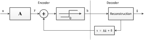
Figure 1: Schematic of one-bit adaptive quantization for compressed sensing.

V-B Adaptive Quantization

As indicated earlier, in addition to the computational issue, the other difficulty we face in developing a practical algorithm is that the suggested optimal quantization thresholds are dependent on the original unquantized data samples $\boldsymbol{y}$ which are inaccessible to the decoder. To overcome this difficulty, we consider an adaptive quantization strategy in which the thresholds are iteratively refined based on the previous estimate/reconstruction.

The basic idea of one-bit adaptive quantization is described as follows. At iteration $t$, we compute the estimated measurements $\boldsymbol{\hat{y}}^{(t)}$ at the decoder based on the sparse signal $\boldsymbol{\hat{x}}^{(t-1)}$ recovered in the previous iteration: $\boldsymbol{\hat{y}}^{(t)}=\boldsymbol{A}\boldsymbol{\hat{x}}^{(t-1)}$. This estimate is then used to update the quantization thresholds: $\boldsymbol{\tau}^{(t)}=\boldsymbol{\hat{y}}^{(t)}+\boldsymbol{\delta}^{(t)}$, where $\boldsymbol{\delta}^{(t)}$ is a vector randomly generated from a certain distribution. In practice, the deviation $\boldsymbol{\delta}^{(t)}$ should be gradually decreased to ensure that the thresholds will eventually come close to $\boldsymbol{y}$. The updated thresholds $\boldsymbol{\tau}^{(t)}$ are then fed back to the encoder. At the encoder, we compare the unquantized measurements $\boldsymbol{y}$ with the updated thresholds $\boldsymbol{\tau}^{(t)}$, and obtain a new set of one-bit measurements $\boldsymbol{b}^{(t)}$, which are sent to the decoder. Based on $\boldsymbol{\tau}^{(t)}$ and the new data $\boldsymbol{b}^{(t)}$, at the decoder, we compute a new estimate of the sparse signal $\boldsymbol{\hat{x}}^{(t)}$ via solving the optimization (43) or (44). A schematic of the proposed adaptive quantization scheme is shown in Fig. 8. Note that throughout this iterative process, the unquantized measurements $\boldsymbol{y}$ are unchanged. For clarity, the one-bit adaptive quantization scheme is summarized as follows.

One-bit adaptive quantization scheme

1. Given an initial estimate $\boldsymbol{\hat{y}}^{(0)}$, and randomly generate an initial deviation vector $\boldsymbol{\delta}^{(0)}$ according to a certain distribution.

2. At iteration $t\geq 0$, let $\boldsymbol{\hat{y}}^{(t)}=\boldsymbol{\hat{y}}^{(0)}$ if $t=0$; otherwise compute $\boldsymbol{\hat{y}}^{(t)}$ as $\boldsymbol{\hat{y}}^{(t)}=\boldsymbol{A}\boldsymbol{\hat{x}}^{(t-1)}$. Based on $\boldsymbol{\hat{y}}^{(t)}$, update the thresholds as: $\boldsymbol{\tau}^{(t)}=\boldsymbol{\hat{y}}^{(t)}+\boldsymbol{\delta}^{(t)}$, where $\boldsymbol{\delta}^{(t)}$ for $t>0$ is randomly generated according to a certain distribution with a decreasing variance. Compare $\boldsymbol{y}$ with the updated thresholds $\boldsymbol{\tau}^{(t)}$ and obtain a new set of one-bit measurements $\boldsymbol{b}^{(t)}$.

3. Based on $\boldsymbol{\tau}^{(t)}$ and $\boldsymbol{b}^{(t)}$, compute a new estimate of the sparse signal $\boldsymbol{\hat{x}}^{(t)}$ via solving the optimization (43) or (44).

4. Go to Step 2 if $\|\boldsymbol{\hat{x}}^{(t)}-\boldsymbol{\hat{x}}^{(t-1)}\|>\omega$, where $\omega$ is a prescribed tolerance value; otherwise stop.

As indicated in [6, 19], an important benefit brought by the one-bit design is the significant reduction of the hardware complexity. One-bit quantizer which takes the form of a simple comparator is particularly appealing in hardware implementations, and can operate at a much higher sampling rate than the high-resolution quantizer. Also, one-bit measurements are much more amiable for large-scale parallel processing than high-resolution data. With these merits, the proposed adaptive architecture enables us to develop data acquisition devices with lower-cost and faster speed, meanwhile achieving reconstruction performance similar to that of using multiple-bit quantizer.

The proposed adaptive quantization scheme shares a similar architecture with the method [18] in that both methods iteratively refine the thresholds using estimates obtained in previous iteration. Nevertheless, the rationale behind these two methods are different. Our proposed adaptive quantization scheme is based on Theorem 1 which suggests that an arbitrarily small reconstruction error can be attained if the thresholds are set close enough to the unquantized measurements $\boldsymbol{y}$, whereas for [18], a similar theoretical guarantee is unavailable.

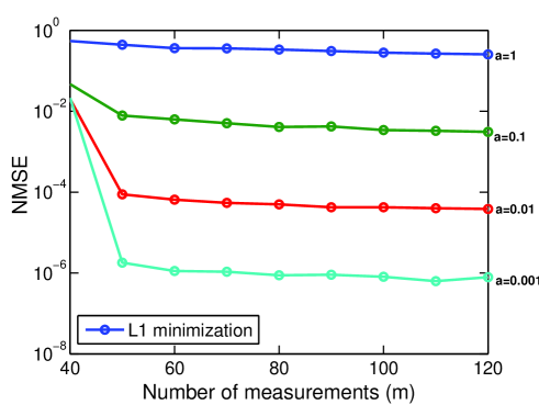
(a) $\ell_{1}$-minimization

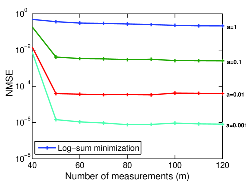
(b) Log-sum minimization

Figure 2: Reconstruction mean-squared error versus the number of measurements for different choices of $a$.

VI Numerical Results

We now carry out experiments to corroborate our previous analysis and to illustrate the performance of the proposed adaptive quantization scheme. In our simulations, the $K$-sparse signal is randomly generated with the support set of the sparse signal randomly chosen according to a uniform distribution. The signals on the support set are independent and identically distributed (i.i.d.) Gaussian random variables with zero mean and unit variance. The measurement matrix $\boldsymbol{A}\in\mathbb{R}^{m\times n}$ is randomly generated with each entry independently drawn from Gaussian distribution with zero mean and unit variance. To circumvent the difficulty of solving (4), we replace the $\ell_{0}$ norm with alternative sparsity-encouraging functionals, namely, $\ell_{1}$ norm and the log-sum penalty function. The new formulated optimization problems (c.f. (43) and (44)) can be efficiently solved.

VI-A Performance under Different Threshold Choices

We first examine the impact of the quantization design on the reconstruction performance. The knowledge of the original unquantized measurements $\boldsymbol{y}$ is assumed available in order to validate our theoretical results. The thresholds are chosen to be the sum of the unquantized measurements $\boldsymbol{y}$ and a deviation term $\boldsymbol{\delta}$, i.e. $\boldsymbol{\tau}=\boldsymbol{y}+\boldsymbol{\delta}$, where $\boldsymbol{\delta}$ is a vector with its entries being independent discrete random variables with $P(\delta_{i}=-a)=0.5$ and $P(\delta_{i}=a)=0.5$, in which the parameter $a>0$ controls the deviation of $\boldsymbol{\tau}$ from $\boldsymbol{y}$. Fig. 2 depicts the reconstruction normalized mean squared error (NMSE), $E[\frac{\|\boldsymbol{x}-\boldsymbol{\hat{x}}\|^{2}}{\|\boldsymbol{x}\|^{2}}]$, vs. the number of measurements $m$ for different choices of $a$, where we set $n=50$, and $K=3$. Results are averaged over $10^{4}$ independent runs. From Fig. 2, we see that the reconstruction performance can be significantly improved by reducing the deviation parameter $a$. In particular, a NMSE as small as $10^{-6}$ can be achieved when $a$ is set $0.001$. This corroborates our theoretical analysis that sparse signals can be recovered with an arbitrarily small error by letting $\boldsymbol{\delta}\rightarrow\boldsymbol{0}$. Also, as expected, the reconstruction error decreases with an increasing number of measurements $m$. Nevertheless, the performance improvement due to an increasing $m$ is mild when $m$ is large. This fact suggests that the choice of quantization thresholds is a more critical factor than the number of measurements in achieving an accurate reconstruction. From Fig. 2, we also see that $\ell_{1}$-minimization and log-sum minimization provide similar reconstruction performance. In Fig. 3, we plot the root mean squared error (RMSE), $E[\|\boldsymbol{x}-\boldsymbol{\hat{x}}\|_{2}]$, as a function of the deviation magnitude $\epsilon=\|\boldsymbol{\delta}\|_{2}=\sqrt{m}a$, where we set $m=100$, $n=120$, $K=2$ and $a$ varies from $10^{-3}$ to $1$. It can be observed that the RMSE decreases proportionally with the value $\epsilon$, which coincides with our theoretical analysis (11).

To further corroborate our analysis, we consider a different way to generate the deviation vector $\boldsymbol{\delta}$, with its entries randomly generated according to a Gaussian distribution with zero mean and variance $\sigma^{2}$. Fig. 4 depicts the NMSE vs. the number of measurements $m$ for different values of $\sigma$. Again, we observe that a more accurate estimate is achieved when the thresholds get closer to the unquantized measurements $\boldsymbol{y}$.

Experiments are also carried out on real world images in order to validate our theoretical results. As it is well-known, images have sparse structures in certain over-complete basis, such as wavelet or discrete cosine transform (DCT) basis. In our experiments, we sample each column of the $256\times 256$ image using a randomly generated measurement matrix $\boldsymbol{A}\in\mathbb{R}^{m\times 256}$. We then quantize each real-valued measurement into one bit of information by using the threshold $\tau_{i}=y_{i}+\delta_{i}$, in which $\delta_{i}$ is drawn from a Gaussian distribution $\mathcal{N}(0,0.01)$. Fig. 5 shows the original image and the reconstructed images based on $m\times 256$ one-bit measurements, where $m$ is equal to 150, 200, and 250, respectively. We see that the images restored from one-bit measurements still provide a decent effect, given that the thresholds are well-designed.

VI-B Performance of Adaptive Quantization Scheme

We now carry out experiments to illustrate the performance of the proposed adaptive quantization algorithm. For simplicity, the algorithm uses the optimization (43) at Step 3 of each iteration. In our experiments, we set $n=50$, $K=2$, $\boldsymbol{\tau}^{(0)}=\boldsymbol{\delta}^{(0)}$ and the threshold vector is updated as $\boldsymbol{\tau}^{(t)}=\boldsymbol{\hat{y}}^{(t)}+\xi^{(t)}\boldsymbol{\delta}^{(t)}$ for $t>0$, where $\boldsymbol{\delta}^{(t)},\forall t$ is a random vector with its entries following a normal distribution with zero mean and unit variance. The parameter $\xi^{(t)}$ controls the magnitude of the deviation error. We set $\xi^{(0)}=1$, and to gradually decrease the deviation error, $\xi^{(t)}$ is updated according to $\xi^{(t+1)}=\xi^{(t)}/10$. The NMSE vs. the number of iterations is plotted in Fig. 6, where we set $m=40$. Results are averaged over $10^{3}$ independent runs, with the sampling matrix and the sparse signal randomly generated for each run. From Fig. 6, we see that the adaptive algorithm provides a consistent performance improvement through iteratively refining the quantization thresholds, and usually provides a reasonable reconstruction performance within only a few iterations. Fig. 7 depicts the NMSEs as a function of the number of measurements for the one-bit adaptive quantization scheme and a non-adaptive one-bit scheme which uses $\boldsymbol{\tau}^{(0)}$ as its thresholds. For the adaptive scheme, the iterative process stops if $\|\boldsymbol{\hat{x}}^{(t)}-\boldsymbol{\hat{x}}^{(t-1)}\|_{2}<0.01$. Numerical results show that the adaptive scheme usually converges within ten iterations. We observe from Fig. 7 that the adaptive scheme presents a clear performance advantage over the non-adaptive method.

We examine the effectiveness of the adaptive quantization scheme for image recovery. In the experiments, we sample each column of the $128\times 128$ image using a randomly generated measurement matrix $\boldsymbol{A}\in\mathbb{R}^{m\times 128}$, and then quantize each real-valued measurement into one bit of information. The initial threshold vector is set to be $\boldsymbol{\tau}^{(0)}=\boldsymbol{y}+\xi^{(0)}\boldsymbol{\delta}^{(0)}$, where $\xi^{(0)}$ is chosen as $\|\boldsymbol{y}\|_{l}/m$ such that the deviation is comparable to the magnitude of entries in $\boldsymbol{y}$. For $t>0$, the threshold is then updated as $\boldsymbol{\tau}^{(t)}=\boldsymbol{\hat{y}}^{(t)}+\xi^{(t)}\boldsymbol{\delta}^{(t)}$, with $\xi^{(t)}=\xi^{(t-1)}/10$. Fig. 8 plots the images reconstructed by the proposed one-bit adaptive scheme and the non-adaptive one-bit scheme which uses $\boldsymbol{\tau}^{(0)}$ as its thresholds, where we set $m=256$. Fig. 8 demonstrates that the adaptive quantization scheme improves the reconstruction of the image significantly.

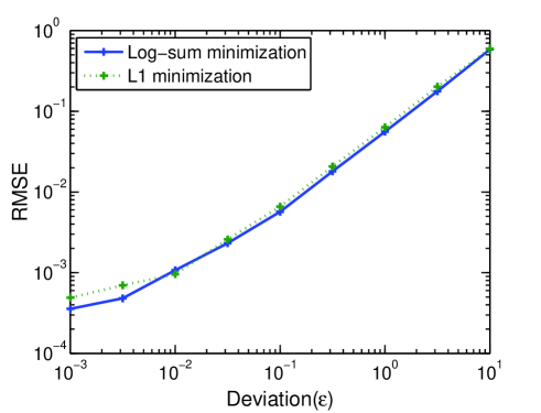
Figure 3: Root mean-squared error versus $\epsilon$.

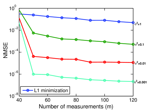
(a) $\ell_{1}$-minimization

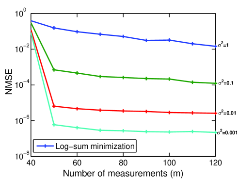
(b) Log-sum minimization

Figure 4: Reconstruction mean-squared error versus the number of measurements for different choices of $\sigma$.

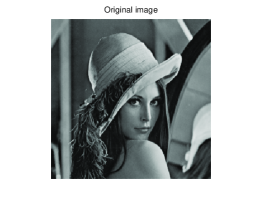
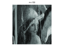
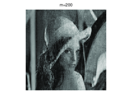
Figure 5: Original image and reconstructed images based on $m\times 256$ one-bit measurements.

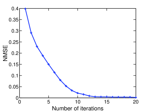
Figure 6: Normalized mean-squared error versus number of iterations.

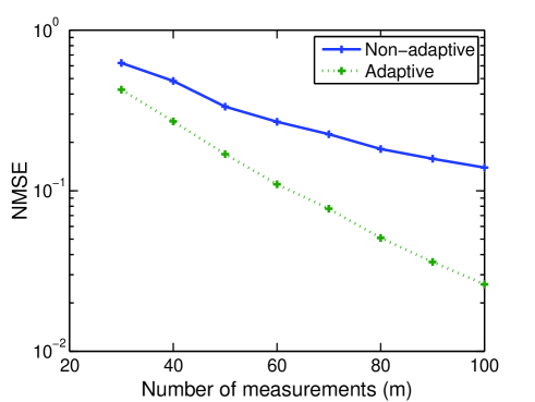
Figure 7: Normalized mean-squared errors versus the number of measurements.

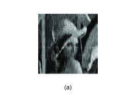
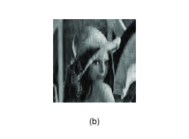
Figure 8: Reconstruction of images from one-bit measurements: (a) Image reconstructed by non-adaptive one-bit scheme; (b) Image reconstructed by adaptive one-bit scheme.

VII Conclusion

We studied the problem of one-bit quantization design for compressed sensing. Specifically, the following two questions were addressed: how to choose quantization thresholds, and how close can the reconstructed signal be to the original signal when the quantization thresholds are well-designed? Our analysis revealed that sparse signals can be recovered with an arbitrarily small error by setting the thresholds close enough to the original unquantized measurements. The unquantized measurements, unfortunately, are inaccessible to us. To address this issue, we proposed an adaptive quantization method which iteratively refines the quantization thresholds based on previous estimate. Simulation results were provided to corroborate our theoretical analysis and to illustrate the effectiveness of the proposed adaptive quantization scheme.

References

- [1] E. Candés and T. Tao, “Decoding by linear programming,” IEEE Trans. Information Theory, no. 12, pp. 4203–4215, Dec. 2005.
- [2] D. L. Donoho, “Compressive sensing,” IEEE Trans. Inform. Theory, vol. 52, pp. 1289–1306, 2006.
- [3] J. A. Tropp and A. C. Gilbert, “Signal recovery from random measurements via orthogonal matching pursuit,” IEEE Trans. Information Theory, vol. 53, no. 12, pp. 4655–4666, Dec. 2007.
- [4] M. J. Wainwright, “Information-theoretic limits on sparsity recovery in the high-dimensional and noisy setting,” IEEE Trans. Information Theory, vol. 55, no. 12, pp. 5728–5741, Dec. 2009.
- [5] I. F. Akyildiz, W. Su, Y. Sankarasubramaniam, and E. Cayirci, “A survey on sensor networks,” IEEE Communications Magazine, pp. 102–114, August 2002.
- [6] J. N. Laska, Z. Wen, W. Yin, and R. G. Baraniuk, “Trust, but verify: fast and accurate signal recovery from 1-bit compressive measurements,” IEEE Trans. Signal Processing, vol. 59, no. 11, pp. 5289–5301, Nov. 2011.
- [7] A. Zymnis, S. Boyd, and E. Candès, “Compressed sensing with quantized measurements,” IEEE Signal Processing Lett., vol. 17, no. 2, pp. 149–152, Feb. 2010.
- [8] T. Wimalajeewa and P. K. Varshney, “Performance bounds for sparsity pattern recovery with quantized noisy random projections,” IEEE Journal on Selected Topics in Signal Processing, vol. 6, no. 1, pp. 43–57, Feb. 2012.
- [9] J. N. Laska and R. G. Baraniuk, “Regime change: bit-depth versus measurement-rate in compressive sensing,” IEEE Trans. Signal Processing, vol. 60, no. 7, pp. 3496–3505, July 2012.
- [10] P. T. Boufounos and R. G. Baraniuk, “One-bit compressive sensing,” in Proceedings of the 42nd Annual Conference on Information Sciences and Systems (CISS 08), Princeton, NJ, 2008.
- [11] L. Jacques, J. N. Laska, P. T. Boufounos, and R. G. Baraniuk, “Robust 1-bit compressive sensing via binary stable embeddings of sparse vectors,” IEEE Trans. Inform. Theory, vol. 59, no. 4, pp. 2082–2102, Apr. 2013.
- [12] P. T. Boufounos, “Greedy sparse signal reconstruction from sign measurements,” in Proceedings of the 43rd Asilomar Conference on Signals, Systems, and Computers (Asilomar 09), Pacific Grove, California, 2009.
- [13] Y. Plan and R. Vershynin, “One-bit compressed sensing by linear programming,” Sep. 2011 [online]. Available: http://arxiv.org/abs/1109.4299.
- [14] M. Yan, Y. Yang, and S. Osher, “Robust 1-bit compressive sensing using adaptive outlier pursuit,” IEEE Trans. Signal Processing, vol. 60, no. 7, pp. 3868–3875, July 2012.
- [15] Y. Shen, J. Fang, H. Li, and Z. Chen, “A one-bit reweighted iterative algorithm for sparse signal recovery,” in IEEE International Conference on Acoustics, Speech, and Signal Processing (ICASSP), Vancouver, Canada, May 26–31 2013.
- [16] J. Z. Sun and V. K. Goyal, “Optimal quantization of random measurements in compressed sensing,” in Proc. IEEE Int. Symp. Information Theory, Seoul, Korea, June 28–July 3 2009.
- [17] U. S. Kamilov, V. K. Goyal, and S. Rangan, “Optimal quantization for compressed sensing under message passing reconstruction,” in Proc. IEEE Int. Symp. Information Theory, Saint Petersburg, Russia, July 31–August 5 2011.
- [18] U. S. Kamilov, A. Bourguard, A. Amini, and M. Unser, “One-bit measurements with adaptive thresholds,” IEEE Signal Processing Lett., vol. 19, no. 10, pp. 607–610, Oct. 2012.
- [19] A. Bourquard, F. Aguet, and M. Unser, “Optical imaging using binary sensors,” vol. 18, no. 5, pp. 4876–4888, Mar. 2010.
- [20] L. Jacques, J. N. Laska, P. T. Boufounos, and R. G. Baraniuk, “Robust 1-bit compressive sensing via binary stable embeddings of sparse vectors,” Apr. 2011 [online]. Available: http://arxiv.org/abs/1104.3160.
- [21] R. R. Coifman and M. Wickerhauser, “Entropy-based algorithms for best basis selction,” IEEE Trans. Inform. Theory, vol. IT-38, pp. 713–718, Mar. 1992.
- [22] E. J. Candes, M. B. Wakin, and S. P. Boyd, “Enhancing sparsity by reweighted minimization,” Journal of Fourier Analysis and Applications, vol. 14, pp. 877–905, Dec. 2008.
- [23] D. Wipf and S. Nagarajan, “Iterative reweighted and methods for finding sparse solutions,” IEEE Journals of Selected Topics in Signal Processing, vol. 4, no. 2, pp. 317–329, Apr. 2010.
- [24] K. Lange, D. Hunter, and I. Yang, “Optimization transfer using surrogate objective functions,” Journal of Computational and Graphical Statistics, vol. 9, no. 1, pp. 1–20, Mar. 2000.