The Mass-Metallicity relation explored with CALIFA:

We present the results on the study of the global and local $\mathcal{M}$-Z relation based on the first data available from the CALIFA survey (150 galaxies). This survey provides integral field spectroscopy of the complete optical extent of each galaxy (up to 2-3 effective radii), with enough resolution to separate individual H ii regions and/or aggregations. Nearly $\sim$3000 individual H ii  regions have been detected. The spectra cover the wavelength range between [OII]3727 and [SII]6731, with a sufficient signal-to-noise to derive the oxygen abundance and star-formation rate associated with each region. In addition, we have computed the integrated and spatially resolved stellar masses (and surface densities), based on SDSS photometric data. We explore the relations between the stellar mass, oxygen abundance and star-formation rate using this dataset.

We derive a tight relation between the integrated stellar mass and the gas-phase abundance, with a dispersion smaller than the one already reported in the literature ($\sigma_{\Delta{\rm log(O/H)}}=$0.07 dex). Indeed, this dispersion is only slightly larger than the typical error derived for our oxygen abundances. However, we do not find any secondary relation with the star-formation rate, other than the one induced due to the primary relation of this quantity with the stellar mass. The analysis for our sample of $\sim$3000 individual H ii  regions confirm (i) the existence of a local mass-metallicity relation and (ii) the lack of a secondary relation with the star-formation rate. The same analysis is done for the specific star-formation rate, with similar results.

Our results agree with the scenario in which gas recycling in galaxies, both locally and globally, is much faster than other typical timescales, like that of gas accretion by inflow and/or metal loss due to outflows. In essence, late-type/disk dominated galaxies seem to be in a quasi-steady situation, with a behavior similar to the one expected from an instantaneous recycling/closed-box model.

1 Introduction

Metals form in stars as a by-product of the thermonuclear reactions that are the central engine of stellar activity. Once they have completed their life cycle, stars eject metals into the interstellar medium, polluting the gas, which is the fuel for the new generation of stars. Therefore, the star-formation rate (SFR), the stellar mass, the metal content and the overall star-formation history of galaxies are strongly interconnected quantities. A fundamental open question in our understanding of galaxy evolution is based on the details of these interconnections (are they local or global? are both intristic or a consequence of the evolution?), and their dependence on other properties of galaxies (are they affected by the environment and how? how does the merging history of the small interactions affect them?).

The existence of a strong correlation between stellar mass and gas-phase metallicity in galaxies is well known (Lequeux et al., 1979; Skillman, 1992). These parameters are two of the most fundamental physical properties of galaxies, both directly related to the process of galaxy evolution. The mass-metallicity ($\mathcal{M}$-Z) relation is consistent with more massive galaxies being more metal-enriched. It was confirmed observationally by Tremonti et al. (2004, hereafter T04), who found a tight correlation spanning over 3 orders of magnitude in mass and a factor of 10 in metallicity, using a large sample of star-forming galaxies up to z $\sim$ 0.1 from the Sloan Digital Sky Survey (SDSS). The $\mathcal{M}$-Z relation appears to be independent of large-scale (Mouhcine et al., 2007) and local environment (Hughes et al., 2012), although it has been observed that in high density environments metallicities are higher than expected (e.g. Mateus et al., 2007; Petropoulou et al., 2012), and in lower density environments satellities have higher metallicities than central galaxies (e.g. Pasquali et al., 2010, 2012). Finally, the relation has been confirmed at all accessible redshifts (e.g. Savaglio et al., 2005; Erb et al., 2006; Maiolino et al., 2008).

Considerable work has been devoted to understanding the physical mechanisms underlying the $\mathcal{M}$-Z relation. The proposed scenarios to explain its origin can be broadly categorized as: 1) the loss of enriched gas by outflows (T04; Kobayashi et al., 2007); 2) the accretion of pristine gas by inflows (Finlator & Davé, 2008); 3) variations of the initial mass function with galaxy mass (Köppen et al., 2007); 4) selective star formation efficiency or downsizing (Brooks et al., 2007; Ellison et al., 2008; Calura et al., 2009; Vale Asari et al., 2009); or a combination of them.

Despite the local nature of the star-formation processes, it has only recently become possible to analyze the $\mathcal{M}$-Z relation for spatially resolved, external galaxies. Early precedents with more limited data include Edmunds & Pagel (1984) and Vila-Costas & Edmunds (1992), who noticed a correlation between mass surface density and gas metallicity in a number of galaxies. Moran et al. (2012) recently reported a correlation between the local stellar mass density and the metallicity valid across all the galaxies in their sample. This result was derived analyzing the individual H ii  regions of a sample of 174 star-forming galaxies, based on slit spectroscopy. We independently confirmed this relation (Rosales-Ortega et al., 2012), using a statistically complete sample of $\sim$2500 H ii  regions extracted from a sample of 38 galaxies, using integral field spectroscopy (IFS), described in Sánchez et al. (2012b).

This local relation is a scaled version of the $\mathcal{M}$-Z relation. This new relation is explained as a simple effect of the inside-out mass/metallicity growth that dominates the secular evolution of late-type galaxies (e.g. Matteucci & Francois, 1989; Boissier & Prantzos, 1999), combined with the fact that more massive regions form stars faster (i.e. at higher SFRs), thus earlier in cosmological times, which can be considered a local downsizing effect, similar to the one observed in individual galaxies (e.g. Pérez-González et al., 2008). This explanation does not require a strong effect of inflows/outflows in shaping the $\mathcal{M}$-Z relation, which can be naturally explained by secular evolution processes.

Recently, evidence has been reported for a dependence of the $\mathcal{M}$-Z relation on the SFR. Different authors found that these three quantities define either a surface or a plane in the corresponding 3D space, i.e., the so-called Fundamental Mass-Metallicity relation (FMR) and/or $\mathcal{M}$-Z-Fundamental Plane, depending on the authors (Lara-López et al., 2010; Mannucci et al., 2010; Yates et al., 2012). Regardless of the actual shape of this relation (Lara-Lopez et al., 2012), its existence is still controversial. The described relationship implies that (i) for the same mass, galaxies with stronger star-formation rates, have lower metallicities, and (ii) for low-mass galaxies, the dependence on the SFR is stronger. Metallicity is a parameter that depends on (i) the star-formation (which enriches galaxies), (ii) inflows (which dilute and reduce the metallicity), and (iii) outflows (which eject metals out of the galaxy). Thus, the reported relation imposes restrictions to the ratio between the chemical enrichment, produced by the SFR, and dynamical timescales which regulates the dilution due to inflows (e.g. Quillen & Bland-Hawthorn, 2008). On the other hand, it also restricts the dependence between the amount of metals ejected by an outflow and the strength of the SFR (Mannucci et al., 2010, and references therein). In a stable situation, described by a simple instantaneous recycling model, no dependence on the SFR is expected.

So far, all the studies reporting a dependence between the $\mathcal{M}$-Z relation and the SFR are based on single aperture spectroscopic data, like the one provided by the SDSS survey (York et al., 2000). In spite of the impressive dataset provided by these surveys, with tens or hundreds of thousands of individual measurements, they present some well-known drawbacks: (i) single aperture spectroscopic data have a fundamental aperture bias, which restricts the derived parameters to different scale-lengths of the galaxies at different redshifts (e.g. Ellis et al., 2005). This is a strong limitation for these studies, considering that both the oxygen abundance and the star-formation rate shows strong gradients within galaxies (e.g. Sánchez et al., 2012b). Therefore, the derived parameters may not be representative of the integrated (or characteristic) ones; (ii) The fact that most of these surveys sample galaxies at a wide range of redshifts implies that the derived parameters correspond to different physical scales, for similar galaxies at different redshift, due to an aperture bias. This may induce secondary correlations difficult to address, in particular, if some of these parameters present a cosmological evolution and/or spatial gradients within each galaxy; (iii) while the spectroscopic information (oxygen abundance and SFR) is derived from this aperture limited dataset, the third analyzed parameter, the mass, is derived mostly based on integrated photometric data. Moreover, in some cases it is derived using the information comprised in the spectroscopic data to estimate the corresponding M/L-ratio (Mannucci et al., 2010; Kauffmann et al., 2003a). Contrary to what is often claimed, we recall that these systematic effects cannot be reduced by the large statistical number of data encompassed in the considered dataset.

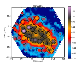
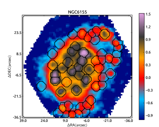
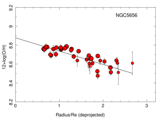
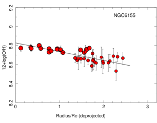
Figure 1: Top panels: IFS-based H$\alpha$ maps, in units of 10^-16 erg s^-1 cm^-2 arcsec^-2, derived for two representative galaxies of the sample (color images), together with the detected H ii regions shown as black segmented contours. Bottom panels: Radial distribution of the oxygen abundance derived for the individual H ii regions with abundace errors below 0.15 dex, as a function of the deprojected distance (i.e., corrected for inclination), normalized to the effective radius, for the same galaxies. The size of the circles is proportional to the H$\alpha$ intensity.

Some of these issues are partially solved when a large aperture is used to derive the spectra of each galaxy, as in the case of drift-scan observations (e.g. Moustakas et al., 2010; Hughes et al., 2012). In this case, the derived abundance (basically luminosity weighted across the optical extent of the galaxies) has a better correspondence with the characteristic one (i.e., the value at 0.4$\rho_{25}$, where $\rho_{25}$ is the radius at a surface brightness of 25 mag/arcsec², Zaritsky et al., 1994; Garnett, 2002), as demonstrated by Moustakas & Kennicutt (2006). On the other hand, the SFR can be directly derived from the integrated H$\alpha$ emission across the considered aperture. However, these observations have also some limitations: (i) in many cases they do not cover the entire optical extent of the galaxies, and the covered fraction is different from galaxy to galaxy, which introduces again an aperture uncertainty (Fig. 3 of Sánchez et al., 2011, for an example); (ii) due to the lack of spatially resolved spectroscopic information, they mix regions with different ionization properties and/or ionization sources, that could change substantially at different locations even within quiescent spiral galaxies (e.g. Sánchez et al., 2012b). This introduces uncertainties in both the derived abundances and the estimated SFR.

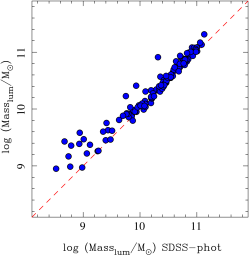
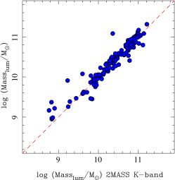
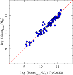
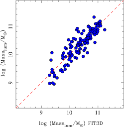
Figure 2: Distribution of the stellar masses derived using the average M/L ratios described in Bell & de Jong (2001) and the $B$ and $V$-band photometry (Y axis in all the panels) along the stellar masses derived using other procedures (X axis in all the panels): Top-Left panels Stellar masses derived using all the five-bands SDSS photometry and the M/L ratio provided by the SED analysis performed using PARADISE; Top-Right panel: Stellar masses derived using the 2MASS K-band photometry and the M/L ratio provided by Longhetti & Saracco (2009); Bottom-left panel: Stellar masses derived using the CALIFA datacubes spectrophotometry and the M/L ratio provided by PyCASSO/Starlight; and Bottom-right panel: Stellar Masses derived from CALIFA datacubes spectrophotometry and the M/L ratio provided by FIT3D

In spite of these limitations, Hughes et al. (2012) explored in a recent study the dependence of the $\mathcal{M}$-Z relation on the SFR, using drift-scan observations of 135 nearby late-type galaxies in the Local Universe. As expected, their dispersion around the $\mathcal{M}$-Z relation is similar or even slightly higher than the one reported by T04. Although, they cannot reproduce the results by Mannucci et al. (2010) and Lara-López et al. (2010), and in fact the scatter increases when they try to introduce a dependence on the SFR, they found a strong depedence of the metallicity with the gas fraction. This dependece could induce a correlation with the SFR in a large sample of galaxies.

More recently, Pérez-Montero et al. (2012) and Cresci et al. (2012) studied the $\mathcal{M}$-Z relation in a wide range of redshifts both using the zCOSMOS data, and the SDSS ones in the first case. They found either a negative trend of the metallicity with the SFR for a fixed galaxy mass, in the first case, or a distribution of masses, metallicies and SFRs consisten with the FMR, in the latter one, both in agreement with Mannucci et al. (2010) and Lara-López et al. (2010). Despite of this agreement, Pérez-Montero et al. (2012) noted that the dispersion around the $\mathcal{M}$-Z relation is only reduced by 0.01 dex at all stellar masses when a secondary relation with the SFR is introduced, for an initial dispersion of $\sim$0.1 dex. As a comparison we should note that the decrease of the dispersion reported by Mannucci et al. (2010) was nearly half of the original value, when introducing the same relation. Pérez-Montero et al. (2012) considered that the lack of extreme SFR values in their SDSS galaxies may explain this effect.

At higher redshifts the situation is more complicated. Wuyts et al. (2012) found that the distribution of their data is in agreement with the local FMR relation presented by Mannucci et al. (2010). However, they do not see a correlation between metallicity and SFR at a fixed mass. On the contrary, Richard et al. (2011) interpret the largest metallicities found at the low mass range as a consequence of the FMR in combination with a lower star-formation rate of these objects. In a similar way, Nakajima et al. (2012) show that the lower limit to the average metallicities found for a sample of Ly$\alpha$ emitters at $z\sim 2.2$, after stacking the individual spectra, is roughly consistent with the FMR relation. Finally, Magrini et al. (2012), support the idea that the scaling relation between the mass, metallicity and SFR has a different origin (and shape) for “active” starbursts, more common at high redshifts, and quiescent galaxies, more frequent at lower ones. The fact that in most cases only the N2 indicator is accesible at high-redshift may introduce biases difficult to quantify.

In order to explore the $\mathcal{M}$-Z relation in the Local Universe, and to bring light to its dependence on the SFR, while minimizing the bias effects previously described, we have used the integral-field spectroscopic (IFS) data provided by the CALIFA survey (Sánchez et al., 2012a). CALIFA is an on-going exploration of the spatially resolved spectroscopic properties of galaxies in the Local Universe ($z<$0.03) using wide-field IFS to cover the full optical extent (up to $\sim$2.5 r_e) of $\sim$600 galaxies of any morphological type, distributed across the entire Color-Magnitude diagram (Walcher et al., in prep.), and sampling the wavelength range 3650-7500Å. So far, the survey has completed $\sim$1/3 of its observations, and the first data release, comprising 100 galaxies has been delivered recently (Husemann et al., 2013).

The layout of this article is as follows: in Sec. 2 we summarize the main properties of the sample and data used in this study; in Sec. 3, we present the main analysis, and the derivation of the parameters analyzed in the article: the mass, metallicity and SFR for each individual galaxy and H ii  region; the global $\mathcal{M}$-Z relation and its dependence with the SFR is explored in Sec. 3.2 and 3.3; a similar analysis for the local $\mathcal{M}$-Z (or $\Sigma$-Z) relation is presented in Sec. 3.4; we explore the possible dependence on the specific star-formation rate (sSFR) in Sec. 3.5; our results and conclusions are summarized in Sec. 4.

2 Sample of galaxies and data

The galaxies under study have been selected from the CALIFA observed sample¹. Since CALIFA is an ongoing survey, whose observations are scheduled on a monthly basis (i.e., dark nights), the list of objects increases regularly. The current results are based on the 150 galaxies observed using the low-resolution setup until July 2012. At that point, most of the color-magnitude diagram had been sampled by the survey with at least one or two targets per bin of magnitude and color, including galaxies of any morphological type. The CALIFA mother sample becomes incomplete below M${}_{r}>-$19 mag, which corresponds to a stellar mass of $\sim$10^9.5 M_⊙. Therefore, it does not sample low-mass and/or dwarf galaxies. Most of these galaxies are part of the 1st CALIFA Data Release Husemann et al. (2013), and therefore the datacube are accesible from the DR1 webpage. Table 1 shows the list of the galaxies analyzed in the current study, including, for each galaxy: (i) its name, (ii) redshift, (iii) $V$-band magnitudes and $B-V$ color and visual morphological classification (extracted from Walcher et al. in prep). In addition, we include the main properties derived along this article, as explained later: (i) the integrated stellar mass, (ii) characteristic oxygen abundance and (iii) the integrated star-formation.

The details of the survey, sample, observational strategy and reduction are explained in Sánchez et al. (2012a). All galaxies were observed using PMAS (Roth et al., 2005) in the PPAK configuration (Kelz et al., 2006), covering a hexagonal field-of-view of 74$\arcsec$$\times$64$\arcsec$, sufficient to cover the full optical extent of the galaxies up to 2-3 effective radii. This is possible due to the diameter selection of the sample (Walcher et al., in prep.). The observing strategy guarantees a complete coverage of the FoV, with a final spatial resolution of FWHM$\sim$3$\arcsec$, i.e., $\sim$1 kpc at the average redshift of the survey. The sampled wavelength range and spectroscopic resolution (3745-7500Å, $\lambda/\Delta\lambda\sim$850, for the low-resolution setup) are more than sufficient to explore the most prominent ionized gas emission lines, from [OII]$\lambda$3727 to [SII]$\lambda$6731, on one hand, and to deblend and subtract the underlying stellar population, on the other hand (e.g. Sánchez et al., 2012a; Kehrig et al., 2012, Cid Fernandes et al., submitted). The dataset was reduced using version 1.3c of the CALIFA pipeline, whose modifications with respect to the one presented in Sánchez et al. (2012a) are described in detail in Husemann et al. (2013). In summary, the data fulfill the foreseen quality control requirements, with a spectrophotometric accuracy better than a 15% everywhere within the wavelength range, both absolute and relative, and a depth that allows us to detect emission lines in individual H ii  regions as weak as $\sim$10^-17erg s^-1 cm^-2 Å^-1, with a S/N$\sim$3-5.

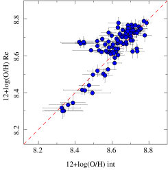
Figure 3: Distribution of the oxygen abundances estimated for each galaxy at the effective radius (Re), using the radial gradients, and the oxygen abundances derived directly from the spectra integrated over the entire field-of-view (int).

The final product of the data-reduction is a regular-grid datacube, with $x$ and $y$ coordinates indicating the right-ascension and declination of the target and $z$ being a common step in wavelength. The CALIFA pipeline also provides the propagated error cube, a proper mask cube of bad pixels, and a prescription of how to handle the errors when doing spatial binning (due to covariance between adjacent pixels after image reconstruction). These datacubes, together with the ancillary data described in Walcher et al. (in preparation), are the basic starting point of our analysis.

In addition to these galaxies, we have included 31 out of the 38 face-on spirals analyzed in Sánchez et al. (2012b). This sample comprises face-on spiral galaxies extracted from the CALIFA feasibility studies (Mármol-Queraltó et al., 2011). All these galaxies were observed with PPAK, using a setup similar to the one used for CALIFA, with slightly different spectral resolutions and wavelength coverage (see Mármol-Queraltó et al., 2011, for details). They cover the same redshift range, optical size and the extent covered by the CALIFA, too. On the other hand, the remaining 7 spirals were extracted from the PINGS survey (Rosales-Ortega et al., 2010). These galaxies are located at lower redshift, being larger in projected sizes, and in some cases they have not been completely covered by the IFS data. Therefore, we prefer to excluded them from this analysis.

3 Analysis and Results

3.1 Derivation of the analyzed parameters

The three main quantities to derive for each galaxy are (i) the integrated stellar mass, (ii) the characteristic oxygen abundance and (iii) the integrated SFR. These parameters were derived following the procedure described in Sánchez et al. (2012b), developed for a similar set of data. In the following we briefly outline the most important aspects of their derivation.

3.1.1 Stellar Masses

We derive the stellar masses using the integrated $V$-band magnitudes and $B-V$ colors listed in Table 1, and the average mass-luminosity ratio ($M/L$) described in Bell & de Jong (2001). The $B$ and $V$-band magnitudes were derived using the Petrosian magnitudes provided the SDSS photometric catalog , and transformed using the equations by Jester et al. (2005). The errors provided by the SDSS catalog were propagated to derive the corresponding errors for the $B$ and $V$-band magnitudes. The expected systematic error of the transformation, of $\sim$0.02 mag, was not taken into account since it will affect equally to all the listed values. . A direct comparison with our own derived magnitudes, based on a growth-curve analysis and a detail subtraction of the local background of the SDSS images shows that the errors could be ad maximum $\sim$0.07 mag (Walcher et al., in prep.) The integrated luminosities and colors were corrected for the effect of dust attenuation, where the internal extinction was derived from the multi-SSP analysis of the stellar continuum summarized in Sánchez et al. (2012a) , prior to derive the stellar masses.

This procedure to derive the stellar masses is robust and straight-forward, and it only requires a few assumptions on the properties of the galaxies. We adopt the Bell & de Jong (2001) $M/L$ ratios, instead of the more recent ones provided by Bell et al. (2003) for the SDSS colors, for consistency with the derivation performed in Sánchez et al. (2012b). Indeed, Bell et al. (2003) show that both $M/L$ ratios are consistent with each other.

In any case, we perform a sanity check to test the robustness of the stellar masses derived. For doing so, we derive the masses using four additional methods: (i) we use the full spectral energy distrubution (SED) provided by the SDSS photometry, and we derive the masses using the stellar population analysis provided by the PARADISE code (Walcher et al., 2011). This derivation is less affected by possible color biases, since it includes the whole optical SEDs. However, the dust attenuation affecting the stellar populations was not taken into account; (ii) we derive the stellar masses using the K-band photometry extracted from the 2MASS photometric catalog , applying a global aperture correction, and adopting the M/L ratio described by Longhetti & Saracco (2009). This derivation is clearly the one that is less affected by any possible color biases, the effect of young stellar populations and dust effects, a priori. However, it presents its own problems, in particlar the uncertainties in the M/L ratio related to the unknown contribution of the TP-AGB stars in this wavelength regime (e.g. Walcher et al., 2011). Only 128 objects from the ones considered here have photometry in the 2MASS catalog; (iii) we collected the stellar masses recently published by Pérez et al. (2013), extracted from the CALIFA datacubes, using pycasso (Cid Fernandes et al., submitted), the 3D implementation of the Starlight code (Cid Fernandes et al., 2005), for those galaxies in common (75 objects). These masses are the most self-consistent with the other parameters presented in this article, but they rely on a less straight-forward stellar population decomposition. The analysis takes into account the dust attenuation; and (iv) we derived the stellar masses provided by the stellar population decomposition method used to remove the underlying stellar population pixel-by-pixel, using FIT3D. This method is, in principle, similar to the previous one. However, FIT3D uses a much more reduced library of stellar populations, and therefore, it provides, a priory, a less accurate M/L ratios and stellar masses.

Figure 2 illustrates the results of this analysis. For each panel, it shows the comparison between the stellar mass derived using the Bell & de Jong (2001) relation, and those ones described before. In all the cases we find a very good agreement, close to a one-to-one relation in most cases. The best agreement is with the stellar masses derived using only photometric information, either the full SDSS SED distribution or the 2MASS K-band data, with a standard deviation of the difference of $\sigma\sim$0.15 dex. The masses derived using only the SDSS photometry are slightly lower, in particular in the low mass regime, which is expected since they are not corrected by dust attenuation. For the stellar masses derived using the CALIFA spectroscopic information, the best agreement is with those provided by pycasso. The standard deviation of the difference is $\sigma\sim$0.14 dex, which is consistent with an spectrophotometric accuracy of the CALIFA datacubes of $\sim$10% with respect to the SDSS one. Finally, the largest dispersion is found when comparing the adopted stellar masses with those derived from the multi-SSP analysis provided by FIT3D ($\sigma\sim$0.24 dex), as expected.

Similar results are found when comparing the masses derived with the total stellar masses listed in the MPA/JHU catalog Kauffmann et al. (2003b). Therefore, if there is a systematic effect in the derivation of the stellar masses, this is at maximum of the order of the typical error estimated based on the propagation of the photometric errors ($\sim$0.15 dex).

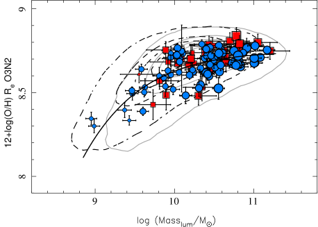
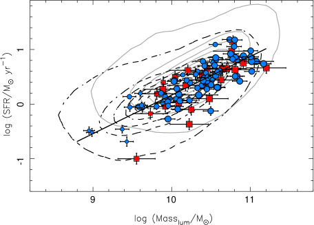
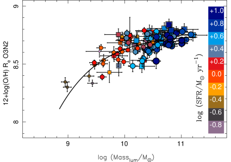
Figure 4: . Top-left panel: Distribution of the oxygen abundances at the effective radii as a function of the integrated stellar masses for the CALIFA galaxies (113, blue solid circles). For comparison purposes, we show similar values for the galaxies observed in the CALIFA feasibility studies (31, red solid squares) included in the H ii regions catalog described in Sánchez et al. (2012b). The size of the symbols is proportional to the integrated SFR. The solid line represents the best fitted curve, as described in the text. We also included the distribution of abundaces as a function of the stellar masses for the SDSS data corresponding to the redshift ranges sampled by Lara-López et al. (2010), dashed black contours, and Mannucci et al. (2010), solid grey contours. In both cases, the first contour encircles the 95% of the objects, and 20% less objects in each consecutive contour. Top-right panel: Distribution of the integrated SFR as a function of the stellar masses. The size of the symbols is proportional to the oxygen abundance shown in previous panel. The solid line represents the best fitted linear regression to the CALIFA data. Like in the previos panel the contours represent the distribution of both parameters corresponding to the redshift ranges sampled by Lara-López et al. (2010), dashed black contours, and Mannucci et al. (2010), solid grey contours Bottom-left panel: Same distribution shown in the top-left panel, for the CALIFA and feasibility-studies objects. The colors represent the logarithm of the integrated SFR for each galaxy. Bottom-right Panel: Distribution of the differential oxygen abundances at the effective radii, once the dependency with the stellar mass has been subtracted, as a function of the integrated SFR for the CALIFA galaxies (113, blue solid circles). The size of the symbols is proportional to the oxygen abundances shown in Fig. 4. The histogram shows the same distribution of differential oxygen abundances. The solid line represents a Gaussian function with the same central value (0.01 dex) and standard deviation (0.07 dex) as the represented distribution, scaled to match the histogram.

3.1.2 Star Formation Rate

The SFR was derived for each galaxy based on the properties of the ionized gas emission. By construction, CALIFA IFS data sample most of the optical extent of galaxies, which allows to derive the total SFR minimizing any aperture effect. The SFR was derived from the integrated H$\alpha$ luminosity. For doing so, we first perform a spectroscopic decomposition analysis between the underlying stellar population and the ionized gas emission lines described using FIT3D (Sánchez et al., 2007b; Rosales-Ortega et al., 2011; Sánchez et al., 2012a, b). The analysis was performed spaxel-by-spaxel, following Sánchez et al. (2011). Each spectrum in the datacube is then decontaminated by the underlying stellar continuum using the multi-SSP model derived . Then, we selected those spaxels whose ionization is dominated by star-formation based on emission line ratios (e.g. Sánchez et al., 2012b), i.e., the H ii  regions described latter. The areas dominated by diffuse gas emission have been excluded on purpose, since their nature is still unclear (e.g. Thilker et al., 2002, , Iglesias-Páramo et al., in prep.). This does not affect the results, since diffuse gas comprises less than 5% of the total integrated flux of H$\alpha$ for our galaxies. We repeated all the calculations using the SFR integrating over all the FoV, instead of just only the H ii  regions without any significant difference. The observed H$\alpha$ intensities were corrected for reddening using the Balmer decrement ($H\alpha/H\beta$) according to the reddening function of Cardelli et al. (1989), assuming $R\equiv A_{V}/E(B-V)=3.1$. The theoretical value for the intrinsic Balmer line ratios were taken from Osterbrock (1989), assuming case B recombination (optically thick in all the Lyman lines), an electron density of $n_{e}=100$ cm^-3 and an electron temperature $T_{e}=10^{4}$ K, which are reasonable assumptions for typical star-forming regions. The values of the SFR were derived for each galaxy adopting the classical relations by Kennicutt (1998), based on the dust-corrected H$\alpha$ luminosities.

The corresponding errors for the SFR were derived, for each galaxy, by propagating through the equations the errors provided by the fitting procedure for the derivation of H$\alpha$ and H$\beta$ emission lines, spaxel-to-spaxel (FIT3D, Sánchez et al., 2011, 2012b). These errors do not include the possible zero-point calibration errors in the CALIFA datacubes, which are estimated to be lower than a $\sim$15% through all the wavelength range (Husemann et al., 2013).

3.1.3 Oxygen Abundance

The characteristic oxygen abundance was defined by Zaritsky et al. (1994) as the abundance at 0.4$\rho_{25}$, being representative of the average value across the galaxy, as we indicated before. This distance corresponds basically to one effective radius for galaxies in the local universe. We demonstrated in Sánchez et al. (2012b), that the effective radius is a convenient parameter to normalize the abundance gradients in galaxies at different redshifts. We will address the study of abundance gradients and the relation between the integrated and characteristic oxygen abundance in a forthcoming article (Sánchez et al. in prep.). Thus, we re-define the characteristic or effective oxygen abundance as the corresponding value at the effective radius.

To derive this parameter we analyze the radial gradients of the oxygen abundance in all the galaxies of our sample, using the procedures detailed in Sánchez et al. (2012b). In a companion article we will describe the procedure for this particular dataset, summarizing the main properties of the ionized regions across the galaxies (Sanchez, in prep.). We present here just a brief summary of the different steps included in the overall process: (i) First we create a narrow-band image of 120$\AA$ width, centered at the wavelength of H$\alpha$ shifted at the redshift of the targets. The narrow-band image is properly corrected for the contamination of the adjacent continuum; (ii) The narrow band image is used as an input for HIIexplorer, an automatic H ii region detection code created for this kind of analysis (Sánchez et al., 2012b; Rosales-Ortega et al., 2012). The code provides with a segmentation map that identifies each detected ionized region. Then, it extracts the integrated spectra corresponding to each segmented region. Figure 1 illustrates the process, showing the H$\alpha$ intensity maps and the corresponding segmentations, for two objects. A total of 3435 individual ionized regions are detected in a total of 137 galaxies from the sample; (iii) Each extracted spectrum is then decontaminated by the underlying stellar continuum using the multi-SSP fitting routines included in FIT3D, as described before; (iv) Then each emission line within the considered wavelength range is fitted with a Gaussian function to recover the line intensities and ratios; (v) These line ratios are used to discriminate between different ionization conditions and to derive the oxygen abundances for each particular ionized region. Basically we selected those clumpy ionized regions with a strong blue underlying stellar population, that contributes at least a 20% of the flux in the $V$-band, to ensure that they are located below the Kewley & Ellison (2008) demarcation line in the classical [OIII]/H$\beta$ vs. [NII]/H$\alpha$ diagnostic diagram (Baldwin et al., 1981). A total of 2846 H ii regions are then extracted, for a total of 134 galaxies; (vi) Finally, in combination with a morphological analysis of the galaxy, we can recover the abundance gradients for each particular galaxy, and derive the corresponding value at the effective radius. For doing so, we fit the radial distribution of the oxygen abundance between 0.2 and 2.1 effective radius with a linear regression, and uses the derived zero-point and slope to determine the oxygen abundance at one effective radius. This procedure increses the accuracy of the derived abundance, since it uses the full radial distribution of individual estimations. We used only (1) those regions for which the oxygen abundance was derived with a nominal error lower than $<$0.2 dex, which corresponds to emission lines with a S/N$>$5 in all the considered emission lines ([OII]3727, H$\beta$, [OIII]5007, H$\alpha$ and [NII]6583), and (2) those galaxies with at least 3 H ii  regions covering at least between 0.3 and 2.1 effective radii. This comprises a total of 2061 H ii regions and associations, distributed in 113 galaxies. This sample comprises galaxies of any type, mostly spirals (both early and late type), with and without bars, and with different inclinations. We note that although the detectability of H ii  regions is affected by inclination, i.e., less number is accesible and detected, we do not notice any further difference in their properties (abundance, radial distribution, luminosity…).

The oxygen abundance was derived using different strong-line indicators, like the R23-fit derived by T04, the N2 and O3N2 calibrators by Pettini & Pagel (2004), and the recently counterpart-method by Pilyugin et al. (2012). Interestingly, despite the differences in the derived estimates, all values show a trend with the stellar mass (e.g. Kewley & Ellison, 2008). In fact, there is a clear correspondence not only with the calibrators (e.g. López-Sánchez et al., 2012), but also between the line ratios used to derive them (e.g. Sánchez et al., 2012b). Therefore, for simplicity, we will show here only the results based on the O3N2-calibrator, which is one of the most straight-forward one.

The results of this analysis are listed in Table 1, including the final number of H ii regions considered for each galaxy and the derived parameters, i.e., the integrated stellar mass and SFR, and characteristic oxygen abundance , together with their corresponding errors. In addition to these characteristic values for each individual galaxy, we derive similar parameters for each individual H ii region: the mass surface density ($\Sigma$) and the surface SFR density ($\mu$SFR). These quantities were derived using the same procedures described in Sec. 3.1.1 and 3.1.2, but using as observables (i.e., the photometric values and the H$\alpha$ fluxes), those ones corresponding to each particular H ii  region. Finally, the derived values were divided by the corresponding encircled area.

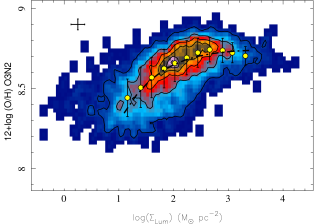
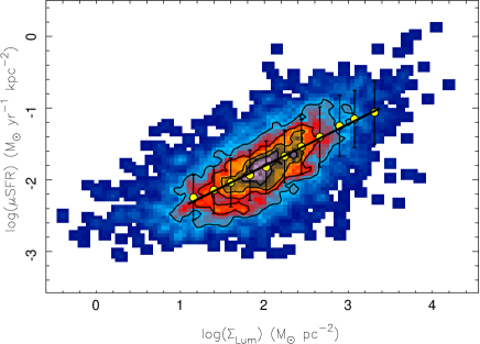
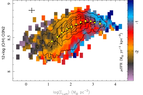
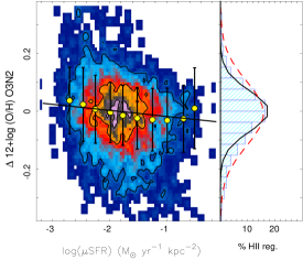
Figure 5: . Top-left panel: Distribution of the oxygen abundances for the 3000 individual H ii regions extracted from the CALIFA data, as a function of the surface mass density, represented with a density contour-plot. The first contour encircles 95% of the total number of H ii regions, with $\sim$20% less in each consecutive contour. The solid-yellow points represent the average oxygen abundances, with their corresponding standard deviations indicated as error bars, for consecutive bins of 0.1 dex in surface mass density. The dot-dashed line represents the best fitted curve for these points. Top-right panel: Distribution of the SFR surface density as a function of the stellar mass density of each individual H ii region. The contour plots represent the density of points in the distribution of oxygen abundances as a function of the surface SFR densities, with the same encircled numbers as in the previous panel. Bottom-left panel: Same distribution shown in the top-left panel, for the CALIFA and feasibility-studies objects. The colors represent the logarithm of the integrated surface density of the SFR for each H ii region. Bottom-right panel: Distribution of the differential oxygen abundance, once the dependency with the surface mass density has been subtracted, for individual H ii regions. The contour plots represent the density of points in the distribution of differential oxygen abundances, once subtracted the dependence on the surface masses densities, as a function of the surface SFR densities, with the same encircled numbers as in the previous panel. The solid-yellow points represent the average values for the abundance offsets, with their corresponding standard deviations indicated as error bars, for consecutive bins of 0.1 dex in surface SFR density.

3.2 Mass Metallicity Relation

We first explore the $\mathcal{M}$-Z relation following T04 and Mannucci et al. (2010). Figure 4 shows the distribution of the characteristic oxygen abundances as a function of the stellar masses for the galaxies of our sample (blue circles). In addition, we have included those values corresponding to the galaxies analyzed in Sánchez et al. (2012b) from the CALIFA feasibility studies (red squares). As expected, there is a clear trend between both quantities, following basically the shape described by Kewley & Ellison (2008) for the considered abundance calibrator. The correlation coefficient between both quantities is $r$=0.769, indicating that there is a positive trend. From the formal point of view, this coefficient should be used only for linear relations. However, it is still valid as an indication of a trend between two parameters.

For comparison purposes, we include the density distribution of galaxies within the $\mathcal{M}$-Z plane for the SDSS galaxies corresponding to the redshift range studied by Lara-López et al. (2010) (dashed black contours) and Mannucci et al. (2010) (solid grey contours). The first contour encircles $\sim$95% of the total number of galaxies, with a 20% decrease in each consecutive one. We have calculated the oxygen abundances for these galaxies using the O3N2 indicator, instead of adopting published metallicities which will force us to adopt a correction. For doing so, the stellar masses and emission line ratios have been directly extracted from the Max-Planck-Institute for Astrophysics-John Hopkins University (MPA-JHU) emission-line analysis database. The contours show that the CALIFA data cover a similar range of masses and metallicities similar to both previous studies. However, it is important to note here that Lara-López et al. (2010) samples a lower mass and higher metallicity range than Mannucci et al. (2010), which is a clear effect of the redshift range covered by both studies and the SDSS selection function.

Instead of the classical polynomial function adopted by most of previous studies for this relation (e.g., T04, Kewley & Ellison, 2008; Mannucci et al., 2010; Rosales-Ortega et al., 2012; Hughes et al., 2012), we prefer to adopt an asymptotic function to describe the relation between both parameters following Moustakas et al. (2011):

$${\rm y}=a+b({\rm x}-c)\exp[-({\rm x}-c)]$$ (1)

Where $y=$ 12+log(O/H), and $x$ is the logarithm of the stellar mass in units of 10⁸M_⊙. This functional form tries to describe the distribution of parameters defining a maximum abundance for large masses ($a$). Although the adopted formula is slightly different for computational convenience than the one adopted by Moustakas et al. (2011), the main motivations and interpretation are the same. Obviously, due to the sample construction, we do not have enough data in the low-mass/low-metallicity range to explore this second range.

The derived parameters for the CALIFA data are $a$=8.74$\pm$0.01, $b$=0.018$\pm$0.007 and $c$=3.5$\pm$0.3. These two latter parameters govern how the metallicity actually increases with mass, while the first one is the asymptotic oxygen abundance for large masses at the effective radius of the galaxies. The derived values cannot be extrapolated to masses lower than 10⁹ M$\odot$, not covered by the CALIFA mother sample. A recent compilation by Kudritzki et al. (2012) of the characteristic metallicities on a set of local universe galaxies indicate that while at high mass they reach an asymptotic value, at low masses the relation is almost linear, consistent with early derivations (e.g. Skillman et al., 1989; Skillman, 1992). With the adopted formula it is possible to reproduce this behavior, although the parameters should be adjusted.

From a theoretical point of view the existence of an asymptotic value is predicted, as proceeding from the production of elements in stars and a given IMF, that is, the stellar true yield for a single stellar population which will be reached when all stars die. An abundance at the effective radius of $\sim$8.74 dex corresponds to a maximum abundance of $\sim$8.84, in the central regions, in agreement with theoretical expectations. For example, Mollá & Díaz (2005) found a saturation level in 12+log(O/H)=8.80. They used a grid of chemical evolution models for spiral and irregular galaxies, the stellar yields by Woosley & Weaver (1995) for oxygen and the IMF by Ferrini et al. (1992). If a different combination of IMF and stellar yield set is used, differences of a factor two may be found. An average value of 8.80$\pm$0.15 would be the maximum oxygen abundance predicted theoretically, which is is also in agreement with more recent estimations Pilyugin et al. (2007).

Since abundance is a relative parameter (amount of oxygen relative to the amount of hydrogen), this value can also be interpreted as the maximum abundance of the universe at a certain redshift. As shown by Moustakas et al. (2011), this parameter evolves with redshift at about $\frac{\Delta log(O/H)}{\Delta z}=-0.2$. The functional form describes well the considered data, as it can be appreciated in Fig. 4. The dispersion of the abundance values along this curve is $\sigma_{\Delta{\rm log(O/H)}}=$0.07 dex, much smaller than previous reported values by (e.g., $\sim$0.1 dex, T04 Mannucci et al., 2010; Hughes et al., 2012). It is important to note here that this dispersion is not much larger than the estimated errors for the characteristic abundances ($e_{\rm log(O/H)}\sim$0.06 dex). Although the dispersion around the correlation depends on the actual form adopted for the $\mathcal{M}$-Z relation, the derived value is always low. If instead of the considered functional form we adopt a 3 or 4 order polynomial function, as the one considered by Kewley & Ellison (2008), the dispersion is just 0.084 dex, smaller than the value reported in that publication for SDSS data using the same calibrator. In any case, our adopted functional form has a more straighforward physical interpretation than the pure polynomial functions adopted in the literature.

The results do not vary significantly when using the oxygen abundance derived from the integrated spectra across the covered FoV. However, both the dispersion around the derived $\mathcal{M}$-Z relation ( $\sim$0.1 dex ) and the estimated errors for the abundances are slightly larger ( $\sim$0.07 dex). This is expected since for the integrated spectra we coadd regions with different ionization sources (e.g. Sánchez et al., 2012b), on one hand, and we have a single estimation of the abundance per object, not a value derived from the analysis of a well defined gradient (which reduces the error in the derivation of the oxygen abundance). Figure 3 illustrates this effect, showing the distribution of the oxygen abundances estimated for each galaxy at the effective radius, using the radial gradients, with the oxygen abundances derived directly from the spectra integrated over the entire field-of-view. As expected both parameters shows a tight correlation ($\sigma\sim$0.06 dex). The errors estimated for the integrated abundance are larger, and they are directly transfereed to the dispersion along the one-to-one relation, and thus, to the corresponding $\mathcal{M}$-Z distribution.

Once this functional form had ben derived, we determined the offset and dispersion for the data corresponding to the galaxies analyzed in Sánchez et al. (2012b). Based also on IFS, and covering the full optical extent of the galaxies, the only possible differences would be either the details of the sample selection and/or the redshift range. The galaxies from the feasibility studies considered here are all face-on spiral galaxies, with an average redshift similar to that of the CALIFA data ($z\sim$0.016), and only slightly larger projected sizes (red squares in Fig. 4). They present a minor offset with respect to the derived $\mathcal{M}$-Z relation ($\Delta log(O/H)=-$0.003 dex) and a slightly larger dispersion ($\sigma_{\Delta log(O/H)}=$0.084 dex). Considering that the spectrophotometric calibration of the data is not that accurate ($\sim$20%, Mármol-Queraltó et al., 2011), the slightly larger redshift range covered by this sample (Sánchez et al., 2012b), and that the sample is smaller (31 objects), the difference is not significant. If we consider both this dataset and the CALIFA one described before, the derived dispersion is just $\sigma_{\Delta log(O/H)}=$0.07.

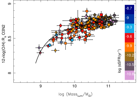
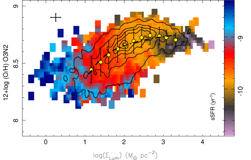
Figure 6: Left panel: Same distribution of the characteristic oxygen abundance as a function of the stellar mass as shown in the bottom panel of Fig. 4. Right panel: Same distribution of the oxygen abundances as a function of the stellar surface density for the individual H ii  regions, as shown in the bottom panel of Fig. 5. In both cases, the color code indicates the logarithm of the specific star formation rate (sSFR).

3.3 Dependence of the $\mathcal{M}$-Z relation on the SFR

The main goal of this study is to explore whether there is a dependence of the $\mathcal{M}$-Z relation on the SFR. Before doing that, it is important to understand the possible additional dependence of the SFR on other properties of the galaxies, in particular on the stellar mass. The SFR of blue/star-forming galaxies has a well known relation with the stellar mass which has been described not only in the Local Universe (e.g. Brinchmann et al., 2004), but also at different redshifts (e.g. Elbaz et al., 2007, and references there in). Its nature is still under debate (e.g. Davé, 2008; Vulcani et al., 2010), but it is most probably related to the ability of a certain galaxy to acquire neutral gas, together with the well known Schmidt-Kennicutt law (Kennicutt, 1998). Regardless of its nature, this relation, together with the $\mathcal{M}$-Z relation may induce a secondary correlation between the SFR and the oxygen abundance.

Figure 4, top-right panel, shows the distribution of the SFR as a function of the stellar mass for both the CALIFA galaxies analyzed here and the galaxies extracted from the feasibility studies. As expected, both parameters show a clear correlation, with a strong correlation coefficient ($r=$0.77). The slope of this relation, for our galaxies, is $\alpha=$0.63, only slightly smaller than the value reported for the Local Universe based on SDSS data ($\sim$0.77, Elbaz et al., 2007). This value is somewhat smaller than the value near to one expected from the simulations (Elbaz et al., 2007). The limited number of low-SFR objects in our sample, may explain the difference in the slope . Nevertheless it is clear that we reproduce the expected correlation . In order to investigate if the selection criteria of the CALIFA galaxies, or the limited number of observed galaxies, have induced any spurious correlation that may affect the distribution of both quantities and/or the described trend, we have compared these distribution with those of the complete SDSS sample for the redshift ranges covered by Lara-López et al. (2010) and Mannucci et al. (2010). For doing so, we uses the MPA-JHU catalog described in the previous section, extracting the same stellar masses and the aperture corrected SFR for both redshift ranges. The distribution of both parameters were represented in Fig. 4, top-right panel, using similar density contours as the ones shown in the top-left panel. It is clear that the ranges of both quantities, and the distribution along the Mass-SFR plane, agree between the three samples. In particular, the agreement is remarkable between our analyzed CALIFA sample and the one studied by Lara-López et al. (2010), which is the one at more similar redshift range. Indeed, the described correlation agrees completely with the SDSS data corresponding to these redshift range. Thus, the selection criteria does not seem to affect neither the range of parameters nor the correlation between both quantities.

Figure 4, bottom-left panel, shows the $\mathcal{M}$-Z relation, but with a different color-coding indicating the integrated SFR of each particular galaxy. There is a trend of the SFR with the metallicity, which follows the trend of the SFR with mass. Thus, more massive galaxies have both higher SFR and are more metal rich. In order to determine which is the dominant correlation, we derive the correlation coefficient between the SFR and the oxygen abundance, obtaining a value of $r=0.54$. This indicates that, while the strength of the $\mathcal{M}$-Z and the SFR-Mass relations are indistinguishable statistically, the SFR-abundance one is weaker, and seems to be induced by the other two.

We do not find any trend between the SFR and the oxygen abundance for a given mass, as the one described by (Lara-López et al., 2010) and Mannucci et al. (2010). For a given mass, the galaxies with stronger star-formation do not seem to have a lower metal content. In order to investigate it further, we derived the differential oxygen abundance with respect to the considered $\mathcal{M}$-Z relation, to search for any correlation with the SFR.

Figure 4, bottom-right panel, shows the distribution of the residual of the oxygen abundance, once the $\mathcal{M}$-Z relation has been subtracted, as a function of the SFR. The data is consistent with being randomly distributed around the zero value, with no correlation between both parameters ($r=0.08$). The histogram of the differential oxygen abundances shows a distribution compatible with a Gaussian function. We recall here that the dispersion around the $\mathcal{M}$-Z relation was just $\sim$0.07 dex, a markedly small error taking into account the nominal errors of the parameters involved. In summary, we cannot confirm the existence of a dependency of the $\mathcal{M}$-Z relation on the SFR, with the current CALIFA data.

A possible concern regarding this result may be that the limited number of objects in the current CALIFA sample may hamper the detection of a significant correlation. We perform a simple Monte-Carlo simulation to test this possibility. For doing so, we assume that the $\mathcal{M}$-Z -SFR distribution follows the analytical formulae described by Mannucci et al. (2010). Then, we extract a random subsample of 100 objects covering a similar range of the parameters covered by the CALIFA sample, and we add a gaussian noise of 0.05 dex (i.e., the value reported by Mannucci et al., 2010). For this subsample, we subtracted the $\mathcal{M}$-Z relation predicted by the same authors, and analyze the possible correlation between the residual of the abundance and the star-formation rate. After 1000 realizations we found that in all the cases we found a clear correlation ($r\sim 0.7$), with an slope compatible with the one predicted by the FMR relation. Thus, the number of objects does not affect the result.

3.4 Dependence of the $\Sigma$-Z relation on the SFR

In Rosales-Ortega et al. (2012) we presented a new scaling relation between the oxygen abundance and the surface mass density for individual H ii regions ($\Sigma$-Z relation) .This relation is a local version of the global $\mathcal{M}$-Z relation, and indeed, it is possible to recover this latter one from the former, just by integrating over a certain aperture (Rosales-Ortega et al., 2012). We proposed that this relation is the real fundamental one and the $\mathcal{M}$-Z relation being a natural consequence. Following this reasoning, it is important to test if there is a secondary relation between the local-$\mathcal{M}$-Z relation and the SFR. An additional advantage of this exploration is the increase of statistical significance of the results, due to the much larger number of sampled objects here ($\sim$3000 H ii regions).

Figure 5, top-left panel, shows the $\Sigma$-Z relation for the H ii  regions of the CALIFA galaxies explored so far. As a first result, we reproduce the relation described in Rosales-Ortega et al. (2012), using a completely different dataset (the catalog of H ii regions extracted from 38 face-on spirals, using IFS data, by Sánchez et al., 2012b). Both quantities have a strong correlation, with a correlation coefficient of $r$=0.98. As in the case of the global $\mathcal{M}$-Z relation, we adopted the asymptotic equation 1. In this case, the $x$ parameter represents the logarithm of the stellar mass surface density in units of M_⊙pc^-2. The $a$, $b$ and $c$ parameters have the same interpretation as those derived for the global relation, and we derive similar values when fitting the data: $a=$8.86$\pm$0.01, $b$=0.97$\pm$0.07 and $c$=2.80$\pm$0.21, reinforcing our hypothesis that both relations are strongly linked. In general, the global-$\mathcal{M}$-Z relation has the same shape as the local one but shifted arbitrarily in mass (to match them to the corresponding mass densities).

Like in the case of the integrated properties of the galaxies, there is a tight correlation between the stellar surface mass density and the surface star-formation density (Fig. 5, top-right panel). The correlation is a clear correlation ($r=0.66$), and it is well described by a simple linear regression. The surface star-formation density scales with the surface mass density with a slope of $\alpha$=0.66$\pm$0.18, once more, below the expected value derived in semi-analytical simulations for the Mass-SFR relation. Note that a comparison with a simulation taking into account the described local relationship is not feasible at present, since no such simulation exists to our knowledge.

This relation indicates that the HII regions with stronger star-formation are located in more massive areas of the galaxies (i.e., towards the center). We have explored if our result is affected by the presence of young stars that biases our mass derivation. However, we found that our surface-brightness and colors (the two parameters used to derive the masses), are not strongly correlated with either the age of the underlying stellar population or the fraction of young stars. Evenmore, the SFR-density presents a positive weak trend with the B-V color, not the other way around.

Like in the global case, these two relations between the oxygen abundance and the surface star-formation rate with the surface mass density, may induce a third relation between the two former parameters. In fact, there is a trend between both parameters, much weaker than the other two described here ($r=0.59$), as expected from an induced correlation. Figure 5 bottom left panel illustrates this dependence, showing the local-$\mathcal{M}$-Z relation, color-coded by the mean surface star-formation rate per bin of oxygen abundance and surface mass density. There is clear gradient in the surface SFR which mostly follows the local-$\mathcal{M}$-Z relation. In this figure we can see a deviation from this global trend in agreement with the results by Lara-López et al. (2010) and Mannucci et al. (2010), in the sense that there are a few H ii  regions with low metal content and high star-formation rate for their corresponding mass surface density (bottom right edge of the figure). However, all together they represent less than a 2-3% of the total sampled regions, and therefore cannot explain a global effect as the one described in those publications. Furthermore, the stochastic fluctuations around the average values at this low number statistics may clearly produce this effect, since there are other H ii  regions in the same location of the diagram with much lower surface SFR.

Following the same procedure outlined in Sec. 3.3, we removed the dependence of the oxygen abundance on the surface mass density by subtracting the derived relation between both parameters. Then, we explore possible dependencies on the surface density SFR. Figure 5, bottom-right panel, illustrates the result of this analysis. It shows the distribution of the differential oxygen abundance along the surface star-formation rate for the individual H ii  regions. No correlation is found between both for the individual values ($r=0.17$). However, the dispersion around the zero-value is larger than that reported for the similar residual distribution for the global relation ($\sigma_{\rm local}=$0.11 dex). The distribution seems to show some tail towards higher abundances for weaker SFRs and lower for stronger ones. Thus, in order to explore possible dependencies even more, we derive average differential oxygen abundance for equal ranges of surface SFR of 0.2 dex width, and determined the correlation coefficient. In this case we found a clearer trend ($r=0.67$), in the sense that H ii  regions with higher surface SFR shows slightly lower abundances for similar masses. However, the slope of the derived regression $\alpha=-$0.0155$\pm$0.217 is compatible with no trend at all, and it is far below the reported value of $\alpha\sim-$0.3 for the dependence of the $\mathcal{M}$-Z relation and the SFR Mannucci et al. (2010) or $\alpha\sim-$0.4 by Lara-López et al. (2010). Applying any of these correlations (i.e., adding $\alpha\cdot$log(SFR) to the mass) does not reduce the dispersion found around the zero value at all ($\sigma_{local,SFR}=$0.108 dex). In summary, we do not find a correlation between the local-$\mathcal{M}$-Z relation with the SFR, in the way described by other authors for the global one. Our results for the local and global $\mathcal{M}$-Z relations are therefore fully consistent.

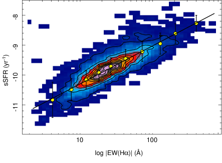
Figure 7: Distribution of the specific star formation as a function of the absolute equivalent width of H$\alpha$, for the individual H ii  regions. The solid yellow circles indicate the location of the average values in bins of 0.2 dex of the equivalent width of H$\alpha$. The solid line shows the best fitted linear regression line

3.5 Dependence of the $\mathcal{M}$-Z relation on the sSFR

Following Mannucci et al. (2010), we have explored the possible dependence of the $\mathcal{M}$-Z relation on the specific star-formation rate (sSFR), a measurement of the current star-formation activity of the galaxy in comparison with the past one. It is known to exhibit a smooth dependence on the stellar mass (sSFR$\propto$M^-1), which has been described at different redshifts (e.g. Elbaz et al., 2007). Many properties of galaxies depend on this parameter. In particular, Mannucci et al. (2010) found that there was an apparent threshold in the sSFR at about 10^-10 yr^-1 which discriminates the effect of the SFR on the $\mathcal{M}$-Z relation, in the sense that the depence is stronger for higher values of the sSFR. In this section we explore the possible dependence of the $\mathcal{M}$-Z on sSFR.

Figure 6 shows both the global and local $\mathcal{M}$-Z relations for the galaxies and H ii  regions discussed in this article. In this case the color code indicates the sSFR, determined by dividing the SFR and stellar masses described before. In both cases the sSFR seems to follow the dependence of the abundance with the mass, without a significant deviation from the trend along this relation. Thus, we do not identify neither a clear secondary dependence on the sSFR, nor a clear threshold at which the global and local $\mathcal{M}$-Z relation show a change in the trend or an offset with respect to the average relation.

In the case of the $\Sigma$-Z relation, the data seem to follow a smooth surface in 3D space, with the three parameters clearly correlated. This surface was already discussed by Rosales-Ortega et al. (2012), who, instead of using the sSFR used the equivalent width of H$\alpha$, a well-known proxy for the former parameter (e.g. Kennicutt, 1998). Figure 7 shows the empirical relation for both parameters based on the individual H ii  regions. The correlation is very strong ($r=0.84$), and well described with a simple linear regression, with a dispersion 0.26 dex:

$${\rm log}({\rm sSFR/yr})=-11.38_{\pm 0.01}+1.23_{\pm 0.02}\cdot{\rm log|EW(H\alpha)/\AA|}$$ (2)

Adopting this relation, the described curve is basically the same as discussed by Rosales-Ortega et al. (2012), considering the reparametrization of one of the axes. We note here that it is required to take the absolute value of the equivalent width of H$\alpha$, which has always negative values for strong emission line regions.

4 Discussion and conclusions

Along this study we have explored the global and local $\mathcal{M}$-Z relations and their possible dependence on the SFR and sSFR based on the ionized gas properties of the first 150 galaxies observed by the CALIFA survey. So far, we have not found any dependence on the SFR and sSFR different than that induced by the well known relation of both parameters with the stellar mass. In addition, we explored similar dependencies for the sample of $\sim$3000 individual H ii  regions extracted from the IFS data. We confirm the $\Sigma$-Z relation described in Rosales-Ortega et al. (2012). However, no secondary dependence is found between this relation and the SFR (or sSFR), different than that induced by their dependences on the stellar mass.

Our results contradict those of Mannucci et al. (2010) and Lara-López et al. (2010), who described a trend for which galaxies with stronger star-formation show lower oxygen abundances for the same mass range. Similar results were already presented by Hughes et al. (2012), using a sample of galaxies observed using drift-scan techniques. The main difference between both datasets is that while Mannucci et al. (2010) and Lara-López et al. (2010) use the spectroscopic data provided by the SDSS (i.e., single aperture, with a strong aperture bias), both Hughes et al. (2012) and the results presented here are based on integrated (and spatially resolved) properties of the galaxies. Shen et al. (2003) show that the physical size of galaxies in the SDSS survey comprises a range of values between a few kpcs to a few tens of kpcs. This means that the SDSS fiber covers a range between $\sim$0.3 and $\sim$10 times the effective radii of galaxies at the redshift range covered by Mannucci et al. (2010) and Lara-López et al. (2010), depending both on their intrinsic properties and the involved cosmological distances. This aperture bias affects mostly the derived SFR (depending on the aperture corretion applied, which are under debate, e.g. Gerssen et al., 2012) and the oxygen abundances (e.g. Sánchez et al., 2012a, b), but in some cases it may also affect the mass derivation (if the spectroscopic information is used to derive the Mass-to-Light ratio).

In addition, the redshift ranges covered by these studies are also different. The data presented by Hughes et al. (2012) and ours are focused on relatively nearby galaxies ($D<120$Mpc), with a narrow range of distances in both cases. In contrast, SDSS data used by Mannucci et al. (2010) and Lara-López et al. (2010) also differ ($0.07<z<0.30$ and $0.04<z<0.1$, respectively), however they both correspond to a much wider redshift range than that covered by us. In both cases the aperture biases of the SDSS spectra have two effects: (i) They grab a larger portion of the galaxies at higher-redshifts, for the same masses, which affects their estimations of the abundance (decreasing the value at higher redshifts) and the SFR (increasing the value at higher redshifts too); (ii) Due to the reported redshift evolution of the $\mathcal{M}$-Z relation, they derive a lower abundance for higher redshift galaxies than for lower-redshift ones, for the same mass, even in the absence of any aperture bias. This second effect may be less important, since it would be at maximum of the order of $\sim$0.06 dex for Mannucci et al. (2010), but just $\sim$0.02 dex for Lara-López et al. (2010). The first effect is also stronger for the case of the study by Mannucci et al. (2010). We can reproduce qualitatively the secondary trend with the SFR of the $\mathcal{M}$-Z relation by taking our IFS data and simulate different SDSS aperture spectra corresponding to different projected distances (see Appendix A). However, the derived slope is not reliable due to the uncertainties involved (different sample selections, different methods to derive the metallicity, unclear evolution of $\mathcal{M}$-Z relation with the redshift). Although we cannot unambiguously prove that aperture effects are inducing this relation, qualitatively there is certainly an agreement.

As described by Mannucci et al. (2010), oxygen abundance is a rather simple parameter, which is governed by three processes: (i) star-formation, which transforms gas into stellar mass, increasing the metal content; (ii) gas accretion, or inflows, which dilutes the oxygen abundance (assuming accretion of more or less pristine gas); and (iii) gas outflows, induced by the star-formation. However, none of these processes is simple, and their interdependence is unclear.

Based on the Schmidt-Kennicutt law, the surface SFR depends on the surface mass density, $\mu{\rm SFR}\propto{\Sigma_{gas}}^{n}$ (Kennicutt, 1998), with a slope larger than one ($n\sim 1.4-1.5$). This means that the integrated SFR of a galaxy should depend on the gas inflow rate (e.g. Mannucci et al., 2010). However, this does not necessarily mean a global dilution and a decrease in the average oxygen abundance, since inflow is a radial process while star-formation is a local one. Gas that falls into the inner regions may be polluted by star formation further out if the latter process is fast enough. Therefore, if the typical timescale to recycle gas is shorter than the inflow timescale (e.g. Silk, 1993), no SFR dependence is expected. On the other hand, if the timescales for the feedback and global gas recycling are much longer than the typical length of a star-formation episode ($\sim$1 Gyr for L^∗ galaxies Quillen & Bland-Hawthorn, 2008), there will be a lose of connection between the starformation and the global metal enrichment, too.

On the other hand, outflows induced by strong star-formation and the subsequent winds due to SN explosions are known to eject metals into the intergalactic medium, and therefore regulate the metal content of galaxies (e.g. Larson, 1974; Prieto et al., 2008; Palacios et al., 2005). It is therefore expected that the strength of the outflows, and the fraction of metals lost, depends on the SFR. However, the detailed relation is difficult to address, since the ability of an outflow to eject metals could be counter-balanced by the gravitational field of the galaxy, which makes metals to fall back into the disk in a back rain process. The high metallicity of the diffuse IGM in galaxy groups and clusters is indirect evidence that at least some fraction of the metals in these winds is lost to the environment (e.g. Renzini et al., 1993).

Although it is hard to study just using the integrated properties of galaxies, the spatial distribution of metals and, in particular, the dispersion of the oxygen abundance at a certain distance from the center could be used to constrain the strength of these (and other) diffusion processes. Our preliminary results, Sánchez et al. (2012b), indicate that this dispersion is rather low. Therefore, either metals are really expelled and lost and/or the net effect is not very strong. The lack of a clear secondary dependence of the oxygen abundance, both globally or locally on the SFR and the $\mu$SFR also suggests that this is not the dominant process.

Following the formalism presented by Mannucci et al. (2010), the fraction of metals ejected due to outflows has to be compensated by the metals produced by the star-formation process. If, instead of the reported dependence of the abundance on the SFR of $\sim-$0.32$\cdot$log(SFR), we consider no dependence at all, and using their formulae, the amount of metals lost by this process should be $\Delta{\rm log(O/H)}\propto$ SFR^0.33, i.e., much smaller than that required to reproduce their results.

In summary our results are consistent with those already presented in Sánchez et al. (2012b) and Rosales-Ortega et al. (2012). In general, the properties of the ionized gas in late-type galaxies are consistent with a quiescent evolution, where gas recycling is faster than other times scales involved (Silk, 1993). This would imply that the galaxies seem to behave locally in a similar manner than globally, dominated by a radial mass distribution following the potential well of the matter, with an inside-out growth that is regulated by gas inflow and local down-sizing star-formation. Therefore, the dominant parameter that defines the amount of metals is the stellar mass, since both parameters are the consequence of an (almost) closed-box star-formation process. However, we should remark that our results are only valid for galaxies with stellar masses higher than $\sim$10^9.5 M_⊙, where the CALIFA sample becomes complete.

Table 1: Properties of the sample of galaxies.

Galaxy	redshift	V-band (mag)	B-V	Type	NHII	log(Mass/M$\odot$)	12+log(O/H)	log(SFR/M$\odot$ yr-1)
IC5376	0.01663	13.84 $\pm$ 0.02	0.89 $\pm$ 0.03	SbA	2	10.55 $\pm$ 0.19	$\cdots$	$\cdots$
NGC7819	0.01730	13.80 $\pm$ 0.02	0.71 $\pm$ 0.03	ScA	31	10.41 $\pm$ 0.17	8.63 $\pm$ 0.07	0.48 $\pm$ 0.01
UGC00036	0.02089	13.72 $\pm$ 0.01	0.95 $\pm$ 0.01	SabAB	5	10.88 $\pm$ 0.20	8.72 $\pm$ 0.04	0.40 $\pm$ 0.01
NGC0001	0.01502	13.11 $\pm$ 0.01	0.85 $\pm$ 0.01	SbcA	31	10.75 $\pm$ 0.19	8.75 $\pm$ 0.06	0.93 $\pm$ 0.01
NGC0036	0.01993	13.06 $\pm$ 0.01	0.93 $\pm$ 0.01	SbB	25	11.08 $\pm$ 0.20	8.71 $\pm$ 0.04	0.76 $\pm$ 0.01
UGC00312	0.01532	13.73 $\pm$ 0.02	0.48 $\pm$ 0.02	SdB	0	10.06 $\pm$ 0.14	$\cdots$	$\cdots$
NGC0444	0.01596	14.34 $\pm$ 0.03	0.63 $\pm$ 0.04	ScdA	11	9.98 $\pm$ 0.16	8.52 $\pm$ 0.06	0.10 $\pm$ 0.01
NGC0477	0.01989	14.05 $\pm$ 0.02	0.81 $\pm$ 0.02	SbcAB	24	10.53 $\pm$ 0.18	8.64 $\pm$ 0.11	0.75 $\pm$ 0.01
IC1683	0.01584	13.67 $\pm$ 0.01	0.88 $\pm$ 0.02	SbAB	4	10.55 $\pm$ 0.19	8.74 $\pm$ 0.03	0.77 $\pm$ 0.01
NGC0496	0.02003	13.71 $\pm$ 0.02	0.68 $\pm$ 0.02	ScdA	30	10.57 $\pm$ 0.17	8.62 $\pm$ 0.07	0.81 $\pm$ 0.01
UGC01057	0.02107	14.23 $\pm$ 0.02	0.62 $\pm$ 0.03	ScAB	21	10.33 $\pm$ 0.16	8.55 $\pm$ 0.15	0.60 $\pm$ 0.01
NGC0776	0.01616	13.00 $\pm$ 0.01	0.90 $\pm$ 0.01	SbB	34	10.91 $\pm$ 0.20	8.77 $\pm$ 0.07	0.88 $\pm$ 0.01
UGC01938	0.02118	14.23 $\pm$ 0.03	0.72 $\pm$ 0.04	SbcAB	15	10.44 $\pm$ 0.17	8.60 $\pm$ 0.08	0.57 $\pm$ 0.01
NGC1056	0.01512	12.56 $\pm$ 0.01	0.92 $\pm$ 0.01	SaA	10	10.06 $\pm$ 0.20	8.62 $\pm$ 0.03	0.18 $\pm$ 0.01
NGC1167	0.01640	12.26 $\pm$ 0.01	0.98 $\pm$ 0.01	S0A	1	11.31 $\pm$ 0.21	$\cdots$	$\cdots$
NGC1349	0.02191	13.02 $\pm$ 0.02	0.88 $\pm$ 0.02	E6A	7	11.13 $\pm$ 0.19	8.71 $\pm$ 0.08	0.35 $\pm$ 0.02
UGC03107	0.02773	14.41 $\pm$ 0.05	0.82 $\pm$ 0.06	SbA	0	10.71 $\pm$ 0.19	$\cdots$	$\cdots$
UGC03253	0.01363	13.30 $\pm$ 0.01	0.71 $\pm$ 0.02	SbB	26	10.38 $\pm$ 0.17	8.70 $\pm$ 0.06	0.32 $\pm$ 0.01
NGC2253	0.01180	12.65 $\pm$ 0.02	0.79 $\pm$ 0.02	SbcB	20	10.59 $\pm$ 0.18	8.76 $\pm$ 0.03	0.29 $\pm$ 0.01
NGC2410	0.01570	12.94 $\pm$ 0.01	0.86 $\pm$ 0.01	SbAB	19	10.83 $\pm$ 0.19	8.65 $\pm$ 0.05	0.81 $\pm$ 0.01
UGC03944	0.01289	13.92 $\pm$ 0.03	0.57 $\pm$ 0.03	SbcAB	34	9.88 $\pm$ 0.16	8.54 $\pm$ 0.12	0.03 $\pm$ 0.01
UGC03995	0.01601	12.82 $\pm$ 0.01	0.77 $\pm$ 0.01	SbB	19	10.84 $\pm$ 0.18	8.67 $\pm$ 0.05	0.51 $\pm$ 0.01
NGC2449	0.01629	13.12 $\pm$ 0.01	0.87 $\pm$ 0.01	SabAB	9	10.83 $\pm$ 0.19	8.77 $\pm$ 0.03	0.33 $\pm$ 0.01
UGC04132	0.01718	13.28 $\pm$ 0.01	0.80 $\pm$ 0.01	SbcAB	11	10.74 $\pm$ 0.18	8.67 $\pm$ 0.06	1.18 $\pm$ 0.01
UGC04461	0.01657	13.87 $\pm$ 0.02	0.55 $\pm$ 0.03	SbcA	19	10.14 $\pm$ 0.15	8.48 $\pm$ 0.10	0.53 $\pm$ 0.01
IC2487	0.01427	13.52 $\pm$ 0.01	0.84 $\pm$ 0.02	ScAB	23	10.51 $\pm$ 0.19	8.65 $\pm$ 0.06	0.44 $\pm$ 0.01
NGC2906	0.01706	12.51 $\pm$ 0.01	0.88 $\pm$ 0.01	SbcA	31	10.34 $\pm$ 0.19	8.79 $\pm$ 0.05	0.17 $\pm$ 0.01
NGC2916	0.01229	12.87 $\pm$ 0.01	0.65 $\pm$ 0.01	SbcA	50	10.41 $\pm$ 0.16	8.72 $\pm$ 0.07	0.47 $\pm$ 0.01
UGC05108	0.02692	14.02 $\pm$ 0.02	0.84 $\pm$ 0.02	SbB	0	10.87 $\pm$ 0.19	$\cdots$	$\cdots$
UGC05358	0.01045	14.99 $\pm$ 0.03	0.64 $\pm$ 0.04	SdB	6	9.36 $\pm$ 0.16	8.41 $\pm$ 0.05	-0.43 $\pm$ 0.02
UGC05359	0.02812	14.38 $\pm$ 0.03	0.73 $\pm$ 0.03	SbB	0	10.65 $\pm$ 0.17	$\cdots$	$\cdots$
UGC05396	0.01778	14.14 $\pm$ 0.02	0.67 $\pm$ 0.03	SbcAB	16	10.23 $\pm$ 0.17	8.62 $\pm$ 0.06	0.39 $\pm$ 0.01
NGC3106	0.02074	13.03 $\pm$ 0.01	0.88 $\pm$ 0.01	SabA	9	11.08 $\pm$ 0.19	8.71 $\pm$ 0.07	0.43 $\pm$ 0.02
NGC3057	0.01506	13.86 $\pm$ 0.03	0.43 $\pm$ 0.03	SdmB	22	8.95 $\pm$ 0.14	8.34 $\pm$ 0.08	-0.49 $\pm$ 0.01
UGC05498NED01	0.02090	14.21 $\pm$ 0.02	0.94 $\pm$ 0.03	SaA	0	10.66 $\pm$ 0.20	$\cdots$	$\cdots$
UGC05598	0.01875	14.46 $\pm$ 0.03	0.71 $\pm$ 0.03	SbA	10	10.19 $\pm$ 0.17	8.60 $\pm$ 0.05	0.44 $\pm$ 0.01
NGC3303	0.02124	13.98 $\pm$ 0.01	0.97 $\pm$ 0.02	S0aAB	0	10.84 $\pm$ 0.20	$\cdots$	$\cdots$
UGC05771	0.02473	13.67 $\pm$ 0.02	0.96 $\pm$ 0.02	E6A	0	11.08 $\pm$ 0.20	$\cdots$	$\cdots$
NGC3381	0.01638	13.03 $\pm$ 0.01	0.54 $\pm$ 0.01	SdB	49	9.58 $\pm$ 0.15	8.64 $\pm$ 0.06	-0.05 $\pm$ 0.01
UGC06036	0.02168	13.64 $\pm$ 0.01	0.98 $\pm$ 0.01	SaA	0	10.99 $\pm$ 0.21	$\cdots$	$\cdots$
UGC06312	0.02103	13.81 $\pm$ 0.02	0.93 $\pm$ 0.02	SabA	4	10.87 $\pm$ 0.20	8.67 $\pm$ 0.04	0.49 $\pm$ 0.01
NGC3614	0.01762	13.15 $\pm$ 0.02	0.77 $\pm$ 0.02	SbcAB	52	9.95 $\pm$ 0.18	8.71 $\pm$ 0.09	0.04 $\pm$ 0.01
NGC3687	0.01829	12.80 $\pm$ 0.01	0.65 $\pm$ 0.01	SbB	53	10.08 $\pm$ 0.17	8.70 $\pm$ 0.05	-0.09 $\pm$ 0.01
NGC3991	0.01171	13.72 $\pm$ 0.01	0.46 $\pm$ 0.01	SmA	1	9.75 $\pm$ 0.14	$\cdots$	$\cdots$
NGC4003	0.02179	13.60 $\pm$ 0.01	0.93 $\pm$ 0.02	S0aB	0	10.95 $\pm$ 0.20	$\cdots$	$\cdots$
UGC07012	0.01030	14.23 $\pm$ 0.02	0.47 $\pm$ 0.02	ScdAB	13	9.47 $\pm$ 0.14	8.49 $\pm$ 0.08	-0.06 $\pm$ 0.01
NGC4047	0.01125	12.44 $\pm$ 0.01	0.68 $\pm$ 0.01	SbcA	47	10.55 $\pm$ 0.17	8.71 $\pm$ 0.07	0.71 $\pm$ 0.01
UGC07145	0.02195	14.32 $\pm$ 0.03	0.71 $\pm$ 0.03	SbcA	20	10.40 $\pm$ 0.17	8.62 $\pm$ 0.13	0.76 $\pm$ 0.01
NGC4185	0.01284	12.87 $\pm$ 0.01	0.79 $\pm$ 0.02	SbcAB	30	10.58 $\pm$ 0.18	8.75 $\pm$ 0.06	0.33 $\pm$ 0.01
NGC4210	0.01893	12.92 $\pm$ 0.01	0.72 $\pm$ 0.01	SbB	56	10.11 $\pm$ 0.17	8.73 $\pm$ 0.06	0.06 $\pm$ 0.01

Table 1: Properties of the sample of galaxies.Continue

Galaxy	redshift	V-band (mag)	B-V	Type	NHII	log(Mass/M$\odot$)	12+log(O/H)	log(SFR/M$\odot$ yr-1)
IC0776	0.01922	14.55 $\pm$ 0.07	0.63 $\pm$ 0.09	SdmA	15	9.43 $\pm$ 0.17	8.33 $\pm$ 0.06	-0.69 $\pm$ 0.02
NGC4470	0.01776	12.66 $\pm$ 0.01	0.52 $\pm$ 0.01	ScA	18	9.87 $\pm$ 0.15	8.59 $\pm$ 0.03	0.20 $\pm$ 0.01
NGC4676A	0.02242	14.31 $\pm$ 0.02	0.94 $\pm$ 0.03		0	10.71 $\pm$ 0.20	$\cdots$	$\cdots$
NGC4711	0.01353	13.49 $\pm$ 0.01	0.69 $\pm$ 0.02	SbcA	0	10.27 $\pm$ 0.17	$\cdots$	$\cdots$
UGC08107	0.02775	13.85 $\pm$ 0.02	0.89 $\pm$ 0.02	SaA	0	11.02 $\pm$ 0.19	$\cdots$	$\cdots$
NGC4961	0.01845	13.39 $\pm$ 0.01	0.48 $\pm$ 0.01	ScdB	37	9.63 $\pm$ 0.14	8.53 $\pm$ 0.10	-0.07 $\pm$ 0.02
NGC5000	0.01844	13.55 $\pm$ 0.02	0.74 $\pm$ 0.02	SbcB	27	10.61 $\pm$ 0.18	8.74 $\pm$ 0.05	0.60 $\pm$ 0.01
UGC08250	0.01729	14.93 $\pm$ 0.04	0.63 $\pm$ 0.05	ScA	6	9.86 $\pm$ 0.16	8.50 $\pm$ 0.06	0.10 $\pm$ 0.01
UGC08267	0.02418	14.44 $\pm$ 0.03	0.91 $\pm$ 0.03	SbAB	2	10.69 $\pm$ 0.20	$\cdots$	$\cdots$
NGC5016	0.01848	12.71 $\pm$ 0.01	0.63 $\pm$ 0.01	SbcA	46	10.09 $\pm$ 0.16	8.75 $\pm$ 0.07	0.18 $\pm$ 0.01
NGC5218	0.01974	12.74 $\pm$ 0.01	0.90 $\pm$ 0.01	SabB	12	10.50 $\pm$ 0.20	8.70 $\pm$ 0.05	0.36 $\pm$ 0.01
UGC08733	0.01772	14.29 $\pm$ 0.03	0.68 $\pm$ 0.03	SdmB	12	9.37 $\pm$ 0.17	8.40 $\pm$ 0.09	-0.47 $\pm$ 0.01
IC0944	0.02310	13.45 $\pm$ 0.01	0.92 $\pm$ 0.02	SabA	0	11.08 $\pm$ 0.20	$\cdots$	$\cdots$
UGC08778	0.01065	13.84 $\pm$ 0.01	0.78 $\pm$ 0.02	SbA	3	9.99 $\pm$ 0.18	8.67 $\pm$ 0.01	-0.44 $\pm$ 0.01
UGC08781	0.02518	13.49 $\pm$ 0.01	0.82 $\pm$ 0.02	SbB	18	11.02 $\pm$ 0.19	8.68 $\pm$ 0.04	0.61 $\pm$ 0.01
NGC5378	0.01977	13.05 $\pm$ 0.01	0.87 $\pm$ 0.01	SbB	6	10.33 $\pm$ 0.19	8.75 $\pm$ 0.03	-0.43 $\pm$ 0.02
NGC5406	0.01791	12.73 $\pm$ 0.01	0.84 $\pm$ 0.01	SbB	49	11.02 $\pm$ 0.19	8.78 $\pm$ 0.06	0.78 $\pm$ 0.01
UGC09067	0.03099	13.96 $\pm$ 0.02	0.66 $\pm$ 0.02	SbcAB	0	10.81 $\pm$ 0.17	$\cdots$	$\cdots$
NGC5614	0.01282	12.16 $\pm$ 0.01	0.95 $\pm$ 0.01	SaA	8	11.06 $\pm$ 0.20	8.72 $\pm$ 0.03	0.23 $\pm$ 0.01
NGC5633	0.01766	12.61 $\pm$ 0.01	0.65 $\pm$ 0.01	SbcA	29	10.04 $\pm$ 0.17	8.77 $\pm$ 0.06	0.43 $\pm$ 0.01
NGC5630	0.01858	13.39 $\pm$ 0.01	0.46 $\pm$ 0.01	SdmB	14	9.60 $\pm$ 0.14	8.39 $\pm$ 0.05	0.20 $\pm$ 0.01
UGC09291	0.01957	13.58 $\pm$ 0.02	0.61 $\pm$ 0.02	ScdA	27	9.81 $\pm$ 0.16	8.60 $\pm$ 0.10	-0.04 $\pm$ 0.01
NGC5656	0.01051	12.48 $\pm$ 0.01	0.70 $\pm$ 0.01	SbA	31	10.46 $\pm$ 0.17	8.72 $\pm$ 0.06	0.49 $\pm$ 0.01
NGC5682	0.01724	14.23 $\pm$ 0.02	0.53 $\pm$ 0.03	ScdB	5	9.22 $\pm$ 0.15	8.41 $\pm$ 0.05	-0.36 $\pm$ 0.01
NGC5720	0.02588	13.68 $\pm$ 0.01	0.76 $\pm$ 0.02	SbcB	6	10.87 $\pm$ 0.18	8.61 $\pm$ 0.06	0.82 $\pm$ 0.01
NGC5732	0.01241	13.83 $\pm$ 0.01	0.57 $\pm$ 0.02	SbcA	24	9.92 $\pm$ 0.15	8.63 $\pm$ 0.12	0.13 $\pm$ 0.01
UGC09476	0.01065	13.33 $\pm$ 0.01	0.66 $\pm$ 0.02	SbcA	46	10.06 $\pm$ 0.17	8.68 $\pm$ 0.05	0.29 $\pm$ 0.01
NGC5735	0.01244	13.37 $\pm$ 0.02	0.75 $\pm$ 0.02	SbcB	52	10.33 $\pm$ 0.18	8.65 $\pm$ 0.10	0.30 $\pm$ 0.01
NGC5772	0.01620	12.88 $\pm$ 0.01	0.82 $\pm$ 0.01	SabA	20	10.87 $\pm$ 0.19	8.74 $\pm$ 0.03	0.42 $\pm$ 0.01
NGC5784	0.01815	12.85 $\pm$ 0.01	0.86 $\pm$ 0.01	S0A	1	11.03 $\pm$ 0.19	$\cdots$	$\cdots$
UGC09598	0.01857	13.94 $\pm$ 0.02	0.74 $\pm$ 0.03	SbcAB	14	10.45 $\pm$ 0.18	8.67 $\pm$ 0.06	0.27 $\pm$ 0.01
UGC09665	0.01838	13.84 $\pm$ 0.02	0.78 $\pm$ 0.02	SbA	7	9.80 $\pm$ 0.18	8.63 $\pm$ 0.03	0.03 $\pm$ 0.01
NGC5829	0.01865	13.86 $\pm$ 0.02	0.59 $\pm$ 0.03	ScA	24	10.31 $\pm$ 0.16	8.53 $\pm$ 0.10	0.55 $\pm$ 0.02
NGC5876	0.01093	12.87 $\pm$ 0.01	0.91 $\pm$ 0.01	S0aB	0	10.55 $\pm$ 0.20	$\cdots$	$\cdots$
NGC5888	0.02902	13.36 $\pm$ 0.01	0.86 $\pm$ 0.02	SbB	0	11.26 $\pm$ 0.19	$\cdots$	$\cdots$
UGC09777	0.01547	14.11 $\pm$ 0.02	0.72 $\pm$ 0.02	SbcA	8	10.19 $\pm$ 0.17	8.65 $\pm$ 0.07	0.33 $\pm$ 0.01
NGC5908	0.01094	12.48 $\pm$ 0.01	1.02 $\pm$ 0.01	SaA	4	10.83 $\pm$ 0.21	8.67 $\pm$ 0.01	0.53 $\pm$ 0.01
NGC5930	0.01861	12.81 $\pm$ 0.01	0.85 $\pm$ 0.01	SabAB	5	10.31 $\pm$ 0.19	8.68 $\pm$ 0.05	0.32 $\pm$ 0.01
UGC09873	0.01844	14.82 $\pm$ 0.04	0.71 $\pm$ 0.05	SbA	5	10.05 $\pm$ 0.17	8.61 $\pm$ 0.06	0.35 $\pm$ 0.01
UGC09892	0.01886	14.46 $\pm$ 0.03	0.72 $\pm$ 0.04	SbcA	7	10.20 $\pm$ 0.17	8.67 $\pm$ 0.06	0.25 $\pm$ 0.01
NGC5953	0.01671	12.64 $\pm$ 0.01	0.84 $\pm$ 0.01	SaA	4	10.10 $\pm$ 0.19	8.70 $\pm$ 0.12	0.10 $\pm$ 0.01
ARP220	0.01813	13.31 $\pm$ 0.01	0.77 $\pm$ 0.02	SdA	0	10.74 $\pm$ 0.18	$\cdots$	$\cdots$
NGC5957	0.01600	12.72 $\pm$ 0.01	0.74 $\pm$ 0.01	SbB	31	9.95 $\pm$ 0.18	8.73 $\pm$ 0.08	-0.27 $\pm$ 0.01
IC4566	0.01846	13.45 $\pm$ 0.01	0.87 $\pm$ 0.02	SbB	6	10.80 $\pm$ 0.19	8.74 $\pm$ 0.07	0.38 $\pm$ 0.01
NGC5987	0.01992	12.35 $\pm$ 0.01	0.96 $\pm$ 0.01	SaA	0	10.73 $\pm$ 0.20	$\cdots$	$\cdots$
UGC10043	0.01715	14.74 $\pm$ 0.07	0.91 $\pm$ 0.09	SabAB	4	9.45 $\pm$ 0.20	8.58 $\pm$ 0.03	-0.66 $\pm$ 0.01
NGC6004	0.01272	12.91 $\pm$ 0.01	0.79 $\pm$ 0.02	SbcB	38	10.56 $\pm$ 0.18	8.78 $\pm$ 0.03	0.52 $\pm$ 0.01
IC1151	0.01712	13.25 $\pm$ 0.01	0.52 $\pm$ 0.01	ScdB	22	9.62 $\pm$ 0.15	8.50 $\pm$ 0.06	-0.02 $\pm$ 0.01
UGC10123	0.01239	13.98 $\pm$ 0.02	0.93 $\pm$ 0.02	SabA	3	10.27 $\pm$ 0.20	8.68 $\pm$ 0.03	0.43 $\pm$ 0.01
NGC6032	0.01424	13.58 $\pm$ 0.02	0.83 $\pm$ 0.02	SbcB	2	10.47 $\pm$ 0.19	$\cdots$	$\cdots$

Table 1: Properties of the sample of galaxies. Continue

Galaxy	redshift	V-band (mag)	B-V	Type	NHII	log(Mass/M$\odot$)	12+log(O/H)	log(SFR/M$\odot$ yr-1)
NGC6060	0.01446	12.74 $\pm$ 0.01	0.82 $\pm$ 0.01	SbA	16	10.81 $\pm$ 0.19	8.69 $\pm$ 0.08	0.86 $\pm$ 0.01
UGC10205	0.02185	13.36 $\pm$ 0.01	0.88 $\pm$ 0.01	S0aA	3	10.99 $\pm$ 0.19	8.63 $\pm$ 0.01	0.52 $\pm$ 0.01
NGC6063	0.01938	13.34 $\pm$ 0.01	0.65 $\pm$ 0.02	SbcA	38	9.96 $\pm$ 0.16	8.61 $\pm$ 0.10	-0.02 $\pm$ 0.01
IC1199	0.01557	13.52 $\pm$ 0.01	0.73 $\pm$ 0.02	SbAB	17	10.45 $\pm$ 0.18	8.77 $\pm$ 0.05	0.42 $\pm$ 0.01
NGC6081	0.01679	13.23 $\pm$ 0.01	0.94 $\pm$ 0.01	S0aA	0	10.87 $\pm$ 0.20	$\cdots$	$\cdots$
UGC10297	0.01757	14.34 $\pm$ 0.02	0.60 $\pm$ 0.03	ScA	5	9.26 $\pm$ 0.16	8.41 $\pm$ 0.09	-0.35 $\pm$ 0.01
UGC10331	0.01589	14.22 $\pm$ 0.03	0.54 $\pm$ 0.03	ScAB	9	9.92 $\pm$ 0.15	8.48 $\pm$ 0.08	0.63 $\pm$ 0.01
NGC6154	0.01993	13.40 $\pm$ 0.01	0.82 $\pm$ 0.02	SabB	15	10.81 $\pm$ 0.19	8.68 $\pm$ 0.04	0.50 $\pm$ 0.01
NGC6155	0.01802	12.87 $\pm$ 0.01	0.64 $\pm$ 0.01	ScA	32	10.03 $\pm$ 0.16	8.72 $\pm$ 0.05	0.42 $\pm$ 0.01
UGC10384	0.01653	14.25 $\pm$ 0.02	0.75 $\pm$ 0.02	SbA	1	10.21 $\pm$ 0.18	$\cdots$	$\cdots$
NGC6168	0.01833	14.27 $\pm$ 0.02	0.65 $\pm$ 0.02	ScAB	11	9.46 $\pm$ 0.16	8.51 $\pm$ 0.05	0.14 $\pm$ 0.01
NGC6186	0.01957	12.89 $\pm$ 0.01	0.83 $\pm$ 0.01	SbB	9	10.36 $\pm$ 0.19	8.78 $\pm$ 0.04	0.48 $\pm$ 0.01
UGC10650	0.01097	15.04 $\pm$ 0.03	0.58 $\pm$ 0.03	ScdA	5	9.27 $\pm$ 0.16	8.40 $\pm$ 0.02	0.06 $\pm$ 0.01
UGC10710	0.02785	14.05 $\pm$ 0.02	0.82 $\pm$ 0.02	SbA	0	10.87 $\pm$ 0.19	$\cdots$	$\cdots$
NGC6310	0.01128	13.19 $\pm$ 0.01	0.82 $\pm$ 0.01	SbA	1	10.39 $\pm$ 0.19	$\cdots$	$\cdots$
UGC10796	0.01040	14.45 $\pm$ 0.03	0.47 $\pm$ 0.03	ScdAB	4	9.39 $\pm$ 0.14	8.44 $\pm$ 0.07	-0.30 $\pm$ 0.02
NGC6361	0.01267	13.06 $\pm$ 0.02	0.99 $\pm$ 0.02	SabA	6	10.73 $\pm$ 0.21	8.68 $\pm$ 0.04	0.98 $\pm$ 0.01
UGC10811	0.02905	14.16 $\pm$ 0.02	0.82 $\pm$ 0.03	SbB	0	10.89 $\pm$ 0.19	$\cdots$	$\cdots$
IC1256	0.01568	13.60 $\pm$ 0.01	0.72 $\pm$ 0.01	SbAB	25	10.40 $\pm$ 0.17	8.76 $\pm$ 0.05	0.42 $\pm$ 0.01
NGC6394	0.02879	14.14 $\pm$ 0.02	0.85 $\pm$ 0.03	SbcB	0	10.89 $\pm$ 0.19	$\cdots$	$\cdots$
UGC10905	0.02580	13.31 $\pm$ 0.01	0.95 $\pm$ 0.02	S0aA	0	11.25 $\pm$ 0.20	$\cdots$	$\cdots$
NGC6478	0.02234	13.76 $\pm$ 0.01	0.82 $\pm$ 0.02	ScA	30	10.79 $\pm$ 0.19	8.67 $\pm$ 0.05	1.06 $\pm$ 0.01
NGC6497	0.02013	13.26 $\pm$ 0.01	0.82 $\pm$ 0.02	SabB	9	10.91 $\pm$ 0.19	8.70 $\pm$ 0.01	0.61 $\pm$ 0.01
UGC11262	0.01836	14.81 $\pm$ 0.04	0.59 $\pm$ 0.05	ScA	8	9.91 $\pm$ 0.16	8.62 $\pm$ 0.04	-0.05 $\pm$ 0.01
NGC6978	0.01986	13.15 $\pm$ 0.02	0.84 $\pm$ 0.02	SbAB	9	10.94 $\pm$ 0.19	8.73 $\pm$ 0.04	0.60 $\pm$ 0.01
UGC11649	0.01249	13.22 $\pm$ 0.03	0.85 $\pm$ 0.03	SabB	18	10.50 $\pm$ 0.19	8.69 $\pm$ 0.09	-0.13 $\pm$ 0.02
UGC11680NED01	0.02649	13.86 $\pm$ 0.02	0.90 $\pm$ 0.03	SbB	10	11.01 $\pm$ 0.20	8.68 $\pm$ 0.06	0.87 $\pm$ 0.01
NGC7047	0.01907	13.41 $\pm$ 0.02	0.83 $\pm$ 0.02	SbcB	0	10.82 $\pm$ 0.19	$\cdots$	$\cdots$
UGC11717	0.02128	13.90 $\pm$ 0.02	1.03 $\pm$ 0.03	SabA	2	10.94 $\pm$ 0.21	$\cdots$	$\cdots$
MCG-01-54-016	0.01062	14.83 $\pm$ 0.05	0.42 $\pm$ 0.06	ScdA	1	9.17 $\pm$ 0.14	$\cdots$	$\cdots$
UGC11740	0.02118	14.26 $\pm$ 0.03	0.71 $\pm$ 0.04	SbcA	9	10.42 $\pm$ 0.17	8.65 $\pm$ 0.03	0.57 $\pm$ 0.01
UGC11792	0.01567	14.49 $\pm$ 0.04	0.75 $\pm$ 0.05	SbcA	4	10.06 $\pm$ 0.18	8.68 $\pm$ 0.01	0.44 $\pm$ 0.01
UGC12054	0.01674	14.42 $\pm$ 0.03	0.51 $\pm$ 0.04	ScA	5	8.97 $\pm$ 0.15	8.32 $\pm$ 0.05	-0.59 $\pm$ 0.01
NGC7311	0.01503	12.19 $\pm$ 0.01	0.88 $\pm$ 0.01	SaA	10	11.17 $\pm$ 0.19	8.75 $\pm$ 0.02	0.72 $\pm$ 0.01
NGC7321	0.02362	13.16 $\pm$ 0.01	0.75 $\pm$ 0.02	SbcB	37	11.01 $\pm$ 0.18	8.71 $\pm$ 0.05	0.98 $\pm$ 0.01
UGC12185	0.02184	13.82 $\pm$ 0.02	0.76 $\pm$ 0.02	SbB	6	10.66 $\pm$ 0.18	8.66 $\pm$ 0.01	0.29 $\pm$ 0.01
UGC12224	0.01171	13.66 $\pm$ 0.03	0.84 $\pm$ 0.04	ScA	48	10.23 $\pm$ 0.19	8.64 $\pm$ 0.08	0.07 $\pm$ 0.01
UGC12308	0.01724	14.56 $\pm$ 0.04	0.45 $\pm$ 0.05	ScdA	10	8.99 $\pm$ 0.14	8.30 $\pm$ 0.08	-0.52 $\pm$ 0.01
NGC7466	0.02489	13.80 $\pm$ 0.02	0.75 $\pm$ 0.02	SbcA	20	10.77 $\pm$ 0.18	8.66 $\pm$ 0.03	0.84 $\pm$ 0.01
NGC7489	0.02072	13.37 $\pm$ 0.02	0.55 $\pm$ 0.02	SbcA	24	10.56 $\pm$ 0.15	8.52 $\pm$ 0.13	1.08 $\pm$ 0.01
NGC7536	0.01540	13.42 $\pm$ 0.02	0.67 $\pm$ 0.03	ScAB	29	10.42 $\pm$ 0.17	8.61 $\pm$ 0.08	0.70 $\pm$ 0.01
NGC7549	0.01549	13.30 $\pm$ 0.01	0.75 $\pm$ 0.02	SbcB	10	10.56 $\pm$ 0.18	8.73 $\pm$ 0.06	0.85 $\pm$ 0.01
NGC7591	0.01633	13.10 $\pm$ 0.01	0.84 $\pm$ 0.02	SbcB	27	10.80 $\pm$ 0.19	8.72 $\pm$ 0.05	1.20 $\pm$ 0.01
UGC12494	0.01318	14.58 $\pm$ 0.05	0.47 $\pm$ 0.06	SdB	0	9.56 $\pm$ 0.14	$\cdots$	$\cdots$
NGC7608	0.01149	14.03 $\pm$ 0.03	0.82 $\pm$ 0.03	SbcA	9	10.06 $\pm$ 0.19	8.73 $\pm$ 0.03	0.08 $\pm$ 0.01
UGC12519	0.01456	13.87 $\pm$ 0.02	0.72 $\pm$ 0.02	ScAB	5	10.22 $\pm$ 0.17	8.59 $\pm$ 0.09	0.57 $\pm$ 0.01
NGC7722	0.01327	12.65 $\pm$ 0.01	1.00 $\pm$ 0.01	SabA	0	10.98 $\pm$ 0.21	$\cdots$	$\cdots$
UGC12864	0.01496	14.12 $\pm$ 0.03	0.65 $\pm$ 0.03	ScB	8	10.03 $\pm$ 0.16	8.53 $\pm$ 0.07	0.18 $\pm$ 0.01
NGC5947	0.01974	13.68 $\pm$ 0.01	0.72 $\pm$ 0.02	SbcB	35	10.58 $\pm$ 0.17	8.66 $\pm$ 0.07	0.59 $\pm$ 0.01
NGC4676B	0.02195	16.55 $\pm$ 0.01	1.07 $\pm$ 0.02	Sbc	2	9.88 $\pm$ 0.22	$\cdots$	$\cdots$

Appendix A Dependence of the $\mathcal{M}$-Z relation with the SFR: Apperture effects.

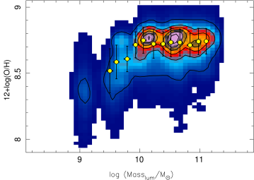
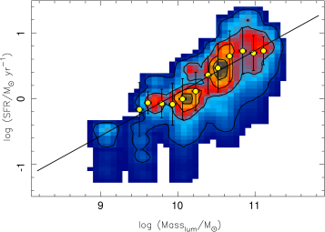
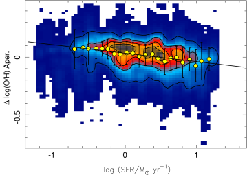
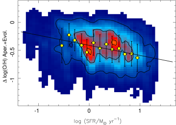
Figure 8: Top-Right panel: Distribution of the oxygen abundance along the stellar mass for the $\sim$50,000 simulated aperture measurements, as described in the text. The contours indicate the same encircled fraction of object than in precendent figures (e.g., Fig. 5). The solid yellow circles indicate the average abundances for consecutive bins of 0.2 dex in stellar mass. Only those binned values with a significant number of objects are shown. Top-left panel: Distribution of the integrated star-formation rate along the stellar mass for the simulated galaxies. Contours and symbols represent the same as in previous panel. The solid line shows the regression line between the two parameters. Bottom-left panel: Distribution of the differential oxygen abundance with respect to the derived $\mathcal{M}$-Z relation along the SFR for the simulated galaxies, when only the aperture effect is considered. Bottom-right panel: Distribution of the differential oxygen abundance with respect to the derived $\mathcal{M}$-Z relation along the SFR for the simulated galaxies, when both the aperture effect and the evolution of the $\mathcal{M}$-Z relation with redshift is taken into account. In both panels the contours and sybmols represent similar concepts like in previous figures and panels. The solid line shows the best derived fit using a simple linear regression method.

We show in the main text our results on the study of the possible dependence of the $\mathcal{M}$-Z relation with the SFR. Using the IFS data provided by the CALIFA survey, we were able to derive the $\mathcal{M}$-Z relation with abundances not affected by aperture effects. In a similar way we derive the complete integrated SFR for these galaxies. Contrary to previous results in the literature (e.g. Mannucci et al. 2010; Lara-López et al. 2010) we find no secondary dependence of the abundance with the SFR once considered the dependence of both parameters with the Mass. The only similar result found in the literature where no dependence on the SFR is described used a sample of integrated spectra taken using drift-scan observations (e.g. Hughes et al. 2012). In summary, when the biases due to aperture are minimized the dependence on the SFR seems to disappear.

It is beyond the scope of this article to explain why other studies find a correlation that we cannot reproduce, in particular when we use a less biased and more detailed estimation of the considered quantities. However, as a sanity check, and in order to provide a suitable explanation, we performed a test of the aperture effects. The oxygen abundance and the SFR are potentially affected by this aperture effect. However, the stellar mass is the less affected, in particular if only photometric data is considered. With CALIFA we are in the unique situation of being able to reproduce the aperture effects present in single aperture observations, by simulating the considered apertures and re-analysing the corresponding simulated spectra.

It is important to use as our starting dataset for the simulations a sample that we know a priori that it does not show any secondary correlation between the abundance and the SFR, when the dependency with the Mass is removed. In this case we will be sure that the induced correlation was not present as an input ingredient of the simulation.

For each galaxy in our dataset with well defined characteristic oxygen abundance, we extracted a set of aperture spectra centred in the peak emission of the galaxy and with consecutive apertures corresponding to the distance of each of the detected H ii  regions from our catalogue. This ensures that there is a clear change in the ionization conditions between consecutive apertures. Each of these aperture spectra correspond to the same galaxy observed at different redshifts. To be consistent with the redshift ranges adopted by Mannucci et al. (2010) and Lara-López et al. (2010), we restricted our apertures to diameters larger than 12$\arcsec$. This roughly corresponds to the projected size of a SDSS fiber at the lower redshift adopted by this study ($z\sim$0.07). Once extracted the spectra, we repeat the same analysis that we perform for the individual H ii  regions, described in Sec. 3.1, deriving the oxygen abundance and integrated SFR. Together with the integrated stellar masses, we ended up with $\sim$2500 individual simulations of the three quantities analysed in this study.

Finally, we perform a Monte-Carlo simulation to take into account the possible effects of the noise in the overall process. For each of the three considered quantities 20 individual realizations were derived, taking into account the corresponding propagated errors (including also those of the stellar masses). We end up with $\sim$50,000 simulated aperture biased quantities.

Figure 8 shows the results of this simulation. In the top-left panel we show the derived $\mathcal{M}$-Z relation for the simulated spectra. As expected it follows the observed relation, presented in Fig. 4. This result was already shown by Rosales-Ortega et al. (2012), where they reproduce the global $\mathcal{M}$-Z from the local one (derived from the abundance gradients), based purely on simulated galaxies. However, a more detailed comparison shows that although both relations are very similar there are slightly differences: (i) the asymptotic oxygen abundance for large masses is $\sim$0.05 dex larger in the simulated relation and (ii) the dispersion of oxygen abundances along the average value is larger ($\sigma_{\rm log(O/H)}\sim$0.1 dex, similar to the one reported by T04). Both results are expected: (1) we are including more central estimations of the abundance for the same range of masses. In the center of the galaxies the abundance is larger than in the outer parts by $\sim$0.1 dex (e.g. Sánchez et al. 2012b). Thus, the net effect is an increase of the upper envelop of the abundance; (2) we are including measurements of different abundances for the same mass range as we enlarge the covered area of the galaxy, simulating the effect of the redshift. Therefore, the dispersion at a certain mass range is increased.

Figure 8, top-righ panel shows the distribution of the simulated SFRs along the stellar masses. As expected we reproduce the relation between both quantities, in a similar way as described in Fig. 4. The main differences are (1) the dispersion is slightly larger: $\sigma_{\rm log(SFR)_{\sim}}\sim$0.35 dex, compared to $\sigma_{\rm log(SFR)}\sim$0.18 dex; (2) there is a tail to lower values of the SFR at a given mass. This is in particular evident for the low-mass range of the figure (${\rm M}\sim 10^{9.5}{\rm M}\odot$). Once more, these effects are clearly explained by the aperture bias, since at a given mass we are sampling areas of lower integrated SFR than the real one (i.e., the central regions), which is an upper envelop.

Finally, we derive the differential oxygen abundance with respect to the considered $\mathcal{M}$-Z relation, for the simulated data. We try to determine if there is any correlation with the SFR, following the analysis in Sec. 3.3. Figure 8, bottom-left panel shows the distribution of these two parameters. There is a clear correlation ($r=0.92$), in the similar sense as described by Mannucci et al. (2010) and Lara-López et al. (2010), i.e., galaxies with lower SFR seem to be more metal poor. Once applied this correlation, we recover the initial dispersion of the $\mathcal{M}$-Z relation described for our original dataset ($\sigma\Delta{\rm log(O/H)}\sim$0.07 dex), a decrease similar to the one reported by these two authors. The dependence of the SFR is $\Delta_{\rm log(O/H)}\propto$$-$0.1 log(SFR), just slightly weaker than the linear term of the equation 2 of Mannucci et al. (2010), $-$0.14 dex/log(SFR), or the combination of equations 3 and 4 of the same authors.

In order to investigate further this issue, we have included in our simulation the reported $\mathcal{M}$-Z evolution with redshift, as described by Moustakas et al. (2011). For doing so, we have determined at which redshift corresponds each of the simulated apertures, and we apply the described correction to the corresponding derived abundance. Results are shown in Figure 8, bottom-right panel. Taking into account the possible redshift dependence, the new differential oxygen abundance have a sharper dependence on the SFR, $\Delta{\rm log(O/H)}$$\propto$$-$0.2log(SFR).

Despite of the fact that this is a very simplistic simulation, based on a reduced number of input galaxies, in general we have shown that aperture effects, together with other evolutionary properties of galaxies, may induce the secondary correlations between the $\mathcal{M}$-Z and the SFR that we are not able to reproduce using our IFS data.