Heavy quark pair production in high
energy pA collisions: Quarkonium

Abstract

Quarkonium production in high-energy proton (deuteron)-nucleus collisions is investigated in the color glass condensate framework. We employ the color evaporation model assuming that the quark pair produced from dense small-$x$ gluons in the nuclear target bounds into a quarkonium outside the target. The unintegrated gluon distribution at small Bjorken $x$ in the nuclear target is treated with the Balitsky-Kovchegov equation with running coupling corrections. For the gluons in the proton, we examine two possible descriptions, unintegrated gluon distribution and ordinary collinear gluon distribution. We present the transverse momentum spectrum and nuclear modification factor for J/$\psi$ production at RHIC and LHC energies, and those for $\Upsilon(1S)$ at LHC energy, and discuss the nuclear modification factor and the momentum broadening by changing the rapidity and the initial saturation scale.

1 Introduction

High-energy proton-nucleus (pA) collisions allow us to explore the dense gluon system appearing at small values of the Bjorken $x$ in the target nucleus. Such a dense gluon system is expected to possess a universal feature of parton saturation, characterized by the saturation momentum scale $Q_{s}^{2}(x)$, and has been investigated with the Color Glass Condensate (CGC) effective theory[1, 2]. In a heavy nucleus with atomic mass number $A$, the saturation phenomenon will become relevant even at moderate $x$ because of its larger gluon density by a factor of target thickness $A^{1/3}$. Very recently p+Pb collisions at the center-of-mass energy $\sqrt{s}=5.02$ TeV have been delivered at the large hadron collider (LHC), and new exciting data are being reported such as hadron multiplicity[3] and ridge phenomenon[4, 5]. The observed hadron multiplicity and momentum spectrum [3] will constrain theoretical models.

At this high energy, the relevant value of $x_{1,2}$ becomes so small that the parton saturation scale $Q_{s}^{2}(x_{2})\propto A^{1/3}x_{2}^{-\lambda}$ with $\lambda\approx 0.3$[6, 7] in the nuclear target will be comparable to or larger than the charm quark mass $m_{c}$. This suggests coherence effects even in charm quark production, and thus we can get useful information of the gluon saturation in the nuclear target by studying the energy and rapidity dependences of charm quark and quarkonium productions in pA collisions at relativistic heavy ion collider (RHIC) and the LHC[8, 9, 10, 11, 12, 13].

In heavy ion collision experiments, heavy quark and quarkonium productions[14, 15] are very valuable probes for quantifying properties of hot and dense matter or a quark-gluon plasma transiently created in the events. Quarkonium suppression[16] and enhancement[17, 18], and energy loss[19, 20, 21] and collective flow of heavy flavor mesons[22] have already been discussed extensively. Here one obviously needs to know the initial nuclear effects on their productions for quantitative understanding of hot-medium modifications.

In this paper we shall investigate phenomenological implications of the saturation effects on the quarkonium production at collider energies by exploiting the color evaporation model (CEM)[15]. Systematic study of quarkonium production spectrum from CGC in pA collisions will quantitatively improve our understanding of gluon saturation effects on particle production in pA collisions. At the same time, it will serve as a benchmark for assessing the hot medium effects on the quarkonium production in AA collisions.

In the CGC framework, the quark-pair production cross section in pA collisions is obtained by Blaizot, Gelis and Venugopalan [23, 24], where pA is treated as a “dilute-dense” system and the cross section is evaluated at leading order in the coupling constant $\alpha_{s}=g^{2}/4\pi$ and the color charge density $\rho_{p}$ in the proton, but in full orders with respect to the color charge density $g^{2}\rho_{A}=O(1)$ in the nucleus. Adopting this formula, we previously evaluated the heavy quark production cross-sections in high-energy pA collisions to reveal their general features[10, 11].

Of particular importance is the $x$ dependence of the unintegrated gluon distribution (uGD) in the nuclear target. We describe the $x$ dependence of uGD with the Balitsky-Kovchegov (BK) equation including the running coupling corrections (rcBK equation)[25]. The BK equation can be derived from a more general equation of functional renormalization group by taking the mean-field approximation. The authors of [26, 27] analyzed the global data of deep inelastic scatterings (DIS) of e+p at HERA using the rcBK equation, to obtain a set of constrained uGD of the proton at small $x<0.01$. The resultant uGD has been applied to compute the particle production at the proton-(anti)proton colliders[28, 29]. We use this constrained uGD in this work.

In forward particle production, the momentum fraction $x_{1}$ of the gluons from the proton is not small, and the distribution may be better described with the ordinary collinear gluon distribution function. Accordingly, the expression of the cross section is obtained by taking the collinear limit ${\boldsymbol{k}}_{1\perp}\to 0$ for the gluon momentum from the proton in the hard matrix element. (This kind of asymmetric treatment is well known for the hadron production from CGC[30].) We will compare the quarkonium production in the collinear approximation on the proton side with the original one that involves the ${\boldsymbol{k}}_{1\perp}$ dependent uGD for the proton.

This paper is organized as follows: In Sec. 2 we review the quark pair production formula in the CGC framework and explain its collinear limit on the proton side. Then we incorporate the $x$-dependence of uGD using the rcBK evolution equation. In Sec. 3, we compute the quarkonium production cross section working in the color evaporation model, and show the transverse momentum spectra and nuclear modification factor for J/$\psi$ at RHIC and LHC energies, and those for $\Upsilon$ at LHC energy. Rapidity and initial-saturation-scale dependences of the nuclear modification factor, and momentum broadening are also discussed. Sec. 4 is devoted to conclusion and outlook.

2 Pair production cross-section

In this section we summarize analytic expressions for the quark-pair production cross-section, derived in Ref. [24]. We also present its limit when the transverse momentum of the gluon coming from the proton is small, in order to make use of conventional collinear factorization for the proton. For more details, see Refs. [24, 11].

2.1 Pair cross-section in the large $N$ limit

In the CGC formalism, the proton-nucleus collision is described as a collision of two sets of color sources representing the large $x$ degrees of freedom in the proton and the nucleus respectively. When they collide, these color sources produce a time-dependent classical color field, and this color field can in turn produce quark-antiquark pairs. Both the classical color field and the quark-pair production amplitude can be calculated analytically when one of the projectiles is dilute and its density of color sources can be treated to the lowest order. This is the approximation we make in the description of proton-nucleus collisions in this framework, the proton naturally being the dilute projectile.

For definiteness, let us denote by $\rho_{p}$ and $\rho_{{}_{A}}$ the densities of color sources in the proton and the nucleus respectively, and that the proton moves in the $+z$ direction and the nucleus in the $-z$ direction. Then, the pair production amplitude reads [24] :

$$\!\!\!\!\!\!\!\!\!\!\!\!{\cal M}_{{}_{F}}({\boldsymbol{q}},{\boldsymbol{p}})\!=\!g^{2}\!\int\!\frac{d^{2}{\boldsymbol{k}}_{1\perp}}{(2\pi)^{2}}\frac{d^{2}{\boldsymbol{k}}_{\perp}}{(2\pi)^{2}}\frac{\rho_{p,a}({\boldsymbol{k}}_{1\perp})}{k_{1\perp}^{2}}\!\int\!\!d^{2}{\boldsymbol{x}}_{\perp}d^{2}{\boldsymbol{y}}_{\perp}e^{i{\boldsymbol{k}}_{\perp}\cdot{\boldsymbol{x}}_{\perp}}e^{i({\boldsymbol{p}}_{\perp}\!+\!{\boldsymbol{q}}_{\perp}\!-\!{\boldsymbol{k}}_{\perp}\!-\!{\boldsymbol{k}}_{1\perp})\cdot{\boldsymbol{y}}_{\perp}}$$

$$\quad\times\overline{u}({\boldsymbol{q}})\Bigg{\{}T_{q\bar{q}}({\boldsymbol{k}}_{1\perp},{\boldsymbol{k}}_{\perp})[{\widetilde{U}}({\boldsymbol{x}}_{\perp})t^{a}{\widetilde{U}}^{\dagger}({\boldsymbol{y}}_{\perp})]+T_{g}({\boldsymbol{k}}_{1\perp})[t^{b}U^{ba}({\boldsymbol{x}}_{\perp})]\Bigg{\}}v({\boldsymbol{p}})\;,$$ (1)

where we denote

$$T_{q\bar{q}}({\boldsymbol{k}}_{1\perp},{\boldsymbol{k}}_{\perp})\equiv\frac{\gamma^{+}(\raise 0.43057pt\hbox{$/$}\kern-5.29999pt\hbox{$q$}-\raise 0.6458pt\hbox{$/$}\kern-5.29999pt\hbox{$k$}+m)\gamma^{-}(\raise 0.43057pt\hbox{$/$}\kern-5.29999pt\hbox{$q$}-\raise 0.6458pt\hbox{$/$}\kern-5.29999pt\hbox{$k$}-\raise 0.6458pt\hbox{$/$}\kern-5.29999pt\hbox{$k$}_{1}+m)\gamma^{+}}{2p^{+}[({\boldsymbol{q}}_{\perp}\!-\!{\boldsymbol{k}}_{\perp})^{2}+m^{2}]+2q^{+}[({\boldsymbol{q}}_{\perp}\!-\!{\boldsymbol{k}}_{\perp}\!-\!{\boldsymbol{k}}_{1\perp})^{2}+m^{2}]}\;,$$

$$T_{g}({\boldsymbol{k}}_{1\perp})\equiv\frac{\raise 0.6458pt\hbox{$/$}\kern-5.29999pt\hbox{$C$}_{{}_{L}}(p+q,{\boldsymbol{k}}_{1\perp})}{(p+q)^{2}}\;,$$ (2)

with ${\boldsymbol{k}}_{2\perp}\equiv{\boldsymbol{p}}_{\perp}+{\boldsymbol{q}}_{\perp}-{\boldsymbol{k}}_{1\perp}$, and where $C_{L}^{\mu}(p+q,{\boldsymbol{k}}_{1\perp})$ is the well-known Lipatov effective vertex. The matrix ${\widetilde{U}}({\boldsymbol{x}}_{\perp})$ is the path-ordered exponential of the gauge field generated by the charge density $\rho_{{}_{A}}$ in the nucleus:

$${\widetilde{U}}({\boldsymbol{x}}_{\perp})\equiv{\cal P}_{+}\exp\left[-ig^{2}\int_{-\infty}^{+\infty}dz^{+}\frac{1}{{\boldsymbol{\nabla}}_{\perp}^{2}}\,\rho_{{}_{A}}(z^{+},{\boldsymbol{x}}_{\perp})\cdot t\right]\,,$$ (3)

with $t^{a}$ the SU($N$) generators in the fundamental representation, and $U({\boldsymbol{x}}_{\perp})$ is the same but in the adjoint representation. The two terms in the curly bracket of Eq. (1) may be interpreted as the processes where a gluon from the proton emits the pair either before or after the collision with the nucleus. The eikonal phases ${\widetilde{U}}$ and $U$ describe the multiple scatterings of a quark or a gluon in the target nucleus. An important property of this amplitude is that the sum of the two terms in the bracket vanishes when ${\boldsymbol{k}}_{1\perp}\to 0$ in agreement with Ward identities [24] – this property is essential in order to recover the limit of collinear factorization on the proton side, which should hold since there is only a single scattering on the proton.

The probability of pair production is then obtained by squaring the above amplitude, and by averaging the squared amplitude with the classical charge distributions of the proton and the nucleus, $W_{p}[x,\rho_{p}]$ and $W_{{}_{A}}[x,\rho_{{}_{A}}]$. The resulting expression generally involves the nuclear multi-parton correlators, e.g., $\langle{\rm tr}\big{(}{\widetilde{U}}({\boldsymbol{x}}_{\perp})t^{a}{\widetilde{U}}^{\dagger}({\boldsymbol{y}}_{\perp}){\widetilde{U}}({\boldsymbol{y}}^{\prime}_{\perp})t^{a}{\widetilde{U}}^{\dagger}({\boldsymbol{x}}^{\prime}_{\perp})\big{)}\rangle_{{}_{Y}}$, where $\langle\cdots\rangle_{{}_{Y}}$ indicates that the average over $\rho_{{}_{A}}$ is performed with the distribution $W_{{}_{A}}[x,\rho_{{}_{A}}]$ evolved to the rapidity $Y\equiv\ln(1/x)$. 2- and 3-point correlators are also needed in the calculation of the pair production probability, but they can be obtained as special cases of the 4-point function thanks to the identity ${\widetilde{U}}({\boldsymbol{x}}_{\perp})t^{a}{\widetilde{U}}^{\dagger}({\boldsymbol{x}}_{\perp})=t^{b}U^{ba}({\boldsymbol{x}}_{\perp})$. This formula also leads to a general sum rule for the Fourier transforms of these correlators $\phi_{{}_{A,Y}}^{q\bar{q},q\bar{q}}$, $\phi_{{}_{A,Y}}^{q\bar{q},g}$ and $\phi_{{}_{A,Y}}^{g,g}$ [24, 11].

All these correlators can be evaluated in a closed form when the distribution of color sources, $W_{{}_{A}}[x,\rho_{{}_{A}}]$, is a Gaussian (see [24]), but the 4-point correlator has a very complicated expression which is quite hard to evaluate numerically. However, in the large $N$ limit, it simplifies into

$${\rm tr}\big{<}{\widetilde{U}}({\boldsymbol{x}}_{\perp})t^{a}{\widetilde{U}}^{\dagger}({\boldsymbol{y}}_{\perp}){\widetilde{U}}({\boldsymbol{u}}_{\perp})t^{a}{\widetilde{U}}^{\dagger}({\boldsymbol{v}}_{\perp})\big{>}_{{}_{Y}} \!\!\!\!\!\mathrel{\mathop{\kern 0.0pt=}\limits_{N\to\infty}} \!\!\!\!\!\frac{N^{2}}{2}S_{{}_{Y}}({\boldsymbol{x}}_{\perp},{\boldsymbol{v}}_{\perp})S_{{}_{Y}}({\boldsymbol{u}}_{\perp},{\boldsymbol{y}}_{\perp})$$ (4)

with

$$S_{{}_{Y}}({\boldsymbol{x}}_{\perp},{\boldsymbol{y}}_{\perp})\equiv{1\over N}{\rm tr}\big{<}{\widetilde{U}}({\boldsymbol{x}}_{\perp}){\widetilde{U}}^{\dagger}({\boldsymbol{y}}_{\perp})\big{>}_{{}_{Y}}\;.$$ (5)

As one can see, it is possible in this limit to write the 4-point (and also the 3-point) function in terms of the 2-point function only, which simplifies considerably all the numerical calculations. Together with the translational invariance in the transverse plane, this fact makes the relation between $\phi_{{}_{A,Y}}^{q\bar{q},q\bar{q}}$ and $\phi_{{}_{A,Y}}^{q\bar{q},g}$ trivial.

By exploiting these relations between the 4-, 3- and 2-point correlators, the pair production probability at the impact parameter ${\boldsymbol{b}}$, in the large $N$ limit, can be written as [11]

$$\frac{dP_{1}({\boldsymbol{b}})}{d^{2}{\boldsymbol{p}}_{\perp}d^{2}{\boldsymbol{q}}_{\perp}dy_{p}dy_{q}}=\frac{\alpha_{s}^{2}N}{8\pi^{4}d_{A}}\frac{1}{(2\pi)^{2}}$$

$$\qquad\times\int\limits_{{\boldsymbol{k}}_{2\perp},{\boldsymbol{k}}_{\perp}}\!\!\frac{\Xi({\boldsymbol{k}}_{1\perp},{\boldsymbol{k}}_{2\perp},{\boldsymbol{k}}_{\perp})}{{\boldsymbol{k}}_{1\perp}^{2}{\boldsymbol{k}}_{2\perp}^{2}}\;\frac{d\phi_{{}_{A},y_{2}}^{q\bar{q},g}({\boldsymbol{k}}_{2\perp},{\boldsymbol{k}}_{\perp};{\boldsymbol{b}})}{d^{2}{\boldsymbol{X}}_{\perp}}\;\varphi_{p,y_{1}}({\boldsymbol{k}}_{1\perp})\;,$$ (6)

where we denote $\int_{{\boldsymbol{k}}_{\perp}}\equiv\int d^{2}{\boldsymbol{k}}_{\perp}/(2\pi)^{2}$, $d_{A}\equiv N^{2}-1$ the dimension of the adjoint representation of $SU(N)$, and ${\boldsymbol{k}}_{1\perp}={\boldsymbol{p}}_{\perp}+{\boldsymbol{q}}_{\perp}-{\boldsymbol{k}}_{2\perp}$. The variables $y_{1,2}$ are the rapidities of the gluons that come from the proton and from the nucleus respectively. A shorthand notation for the squared matrix element is introduced as

$$\Xi({\boldsymbol{k}}_{1\perp},{\boldsymbol{k}}_{2\perp},{\boldsymbol{k}}_{\perp}) = {\rm tr}_{\rm d}\Big{[}(\raise 0.43057pt\hbox{$/$}\kern-5.29999pt\hbox{$q$}\!+\!m)T_{q\bar{q}}(\raise 0.43057pt\hbox{$/$}\kern-6.30005pt\hbox{$p$}\!-\!m)\gamma^{0}T_{q\bar{q}}^{\dagger}\gamma^{0}\Big{]}$$ (7)

$$+{\rm tr}_{\rm d}\Big{[}(\raise 0.43057pt\hbox{$/$}\kern-5.29999pt\hbox{$q$}\!+\!m)T_{q\bar{q}}(\raise 0.43057pt\hbox{$/$}\kern-6.30005pt\hbox{$p$}\!-\!m)\gamma^{0}T_{g}^{\dagger}\gamma^{0}+{\rm h.c.}\Big{]}$$

$$+{\rm tr}_{\rm d}\Big{[}(\raise 0.43057pt\hbox{$/$}\kern-5.29999pt\hbox{$q$}\!+\!m)T_{g}(\raise 0.43057pt\hbox{$/$}\kern-6.30005pt\hbox{$p$}\!-\!m)\gamma^{0}T_{g}^{\dagger}\gamma^{0}\Big{]}\;.$$

In Eq. (6), $\varphi_{p,y_{1}}$ is the uGD in the proton, and ${d\phi_{{}_{A},y_{2}}^{q\bar{q},g}}/{d^{2}{\boldsymbol{X}}_{\perp}}$ is expressed in terms of the Fourier transform of the 3-point nuclear correlator as :

$$\frac{d\phi_{{}_{A},_{Y}}^{q\bar{q},g}({\boldsymbol{l}}_{\perp},{\boldsymbol{k}}_{\perp};{\boldsymbol{X}}_{\perp})}{d^{2}{\boldsymbol{X}}_{\perp}} \equiv \frac{{\boldsymbol{l}}^{2}_{\perp}}{2N\alpha_{s}}\;\int\limits_{{\boldsymbol{x}}_{\perp},{\boldsymbol{y}}_{\perp}}e^{i{\boldsymbol{k}}_{\perp}\cdot({\boldsymbol{x}}_{\perp}-{\boldsymbol{x}}^{\prime}_{\perp})}e^{i({\boldsymbol{l}}_{\perp}-{\boldsymbol{k}}_{\perp})\cdot({\boldsymbol{y}}_{\perp}-{\boldsymbol{x}}^{\prime}_{\perp})}$$ (8)

$$\quad\times\langle{\rm tr}\big{(}\tilde{U}({\boldsymbol{x}}_{\perp})t^{a}\tilde{U}^{\dagger}({\boldsymbol{y}}_{\perp})\tilde{U}({\boldsymbol{x}}^{\prime}_{\perp})t^{a}\tilde{U}^{\dagger}({\boldsymbol{x}}^{\prime}_{\perp})\big{)}\rangle_{{}_{Y}}$$

$$\mathrel{\mathop{\kern 0.0pt=}\limits_{{\rm large}~{}N}} \frac{N{\boldsymbol{l}}^{2}_{\perp}}{4\alpha_{s}}\;S_{{}_{Y}}({\boldsymbol{k}}_{\perp})\;S_{{}_{Y}}({\boldsymbol{l}}_{\perp}-{\boldsymbol{k}}_{\perp})\;,$$

where $S_{{}_{Y}}({\boldsymbol{k}}_{\perp})$ is the Fourier transform of $S_{{}_{Y}}({\boldsymbol{x}}_{\perp})$. The ${\boldsymbol{X}}_{\perp}$ dependence is rather weak for a large nucleus and may be treated implicitly through the variations of saturation scale $Q_{s,A}^{2}({\boldsymbol{X}}_{\perp})$ with ${\boldsymbol{X}}_{\perp}$. In the second line of Eq. (8), we have ignored the ${\boldsymbol{X}}_{\perp}$-dependence of $\phi_{A,y}^{q\bar{q},g}$ when doing the ${\boldsymbol{X}}_{\perp}$ integration because the proton radius is small compared with that of a heavy nucleus ($R_{p}\ll R_{{}_{A}}$). We thus have a compact expression for the quark production probability, but our formula involves a nuclear 3-point function $\phi_{{}_{A},y}^{q\bar{q},g}$, which violates the usual form for $k_{\perp}$-factorization even in the leading order approximation[24, 10].

The pair cross-section in the minimum-bias pA collision is obtained by integrating Eq. (6) over the impact parameter ${\boldsymbol{b}}$. Dividing the cross-section with the total inelastic cross-section $\sigma_{hadr}^{\rm pA}$, which we estimate as $\sigma_{hadr}^{\rm pA}=\pi(R_{A}+R_{p})^{2}\approx\pi R_{A}^{2}$, we have the average multiplicity per event :

$$\frac{dN_{q\bar{q}}}{d^{2}{\boldsymbol{p}}_{\perp}d^{2}{\boldsymbol{q}}_{\perp}dy_{p}dy_{q}} \!\!\!\!\!= \!\!\!\!\!\frac{1}{\pi R_{A}^{2}}\frac{\alpha_{s}^{2}N}{8\pi^{4}d_{A}}\frac{1}{(2\pi)^{2}}\int\limits_{{\boldsymbol{k}}_{2\perp},{\boldsymbol{k}}_{\perp}}\!\!\!\frac{\Xi({\boldsymbol{k}}_{1\perp},{\boldsymbol{k}}_{2\perp},{\boldsymbol{k}}_{\perp})}{{\boldsymbol{k}}_{1\perp}^{2}{\boldsymbol{k}}_{2\perp}^{2}}\;\phi_{{}_{A},y_{2}}^{q\bar{q},g}({\boldsymbol{k}}_{2\perp},{\boldsymbol{k}}_{\perp})\;\varphi_{p,y_{1}}({\boldsymbol{k}}_{1\perp})\;.$$

Here we have introduced the 3-point function integrated over nuclear transverse area

$$\phi_{{}_{A},_{Y}}^{q\bar{q},g}({\boldsymbol{l}}_{\perp},{\boldsymbol{k}}_{\perp}) = \pi R_{A}^{2}\;\frac{N{\boldsymbol{l}}^{2}_{\perp}}{4\alpha_{s}}\;S_{{}_{Y}}({\boldsymbol{k}}_{\perp})\;S_{{}_{Y}}({\boldsymbol{l}}_{\perp}-{\boldsymbol{k}}_{\perp})\;,$$ (10)

which is related to the uGD (2-point function) of the nucleus by $\phi_{{}_{A},_{Y}}^{g,g}({\boldsymbol{l}}_{\perp})=\int_{{\boldsymbol{k}}_{\perp}}\phi_{{}_{A},_{Y}}^{q\bar{q},g}({\boldsymbol{l}}_{\perp},{\boldsymbol{k}}_{\perp})$. The proton uGD $\varphi_{p,y}$ may be estimated by replacing the transverse area $\pi R_{A}^{2}$ and the amplitude $S_{Y}$ with those for the proton.

2.2 Collinear limit on the proton side

When the momentum fraction $x_{1}$ probed in the proton is not small (e.g., $x_{1}>10^{-3}$), and even more so in the forward rapidity region where $x_{1}={\cal O}(1)$, the typical transverse momentum of the gluons in the proton is much smaller than the transverse mass of the produced quark or antiquark, $m_{{\boldsymbol{p}}\perp}\gg k_{1\perp}={\cal O}(\Lambda_{{}_{\rm QCD}})$. We can therefore neglect ${\boldsymbol{k}}_{1\perp}$ in the matrix element $\Xi$ in Eq. (7), and take the collinear approximation on the proton side. This limit is well defined thanks to the fact that the expression on the second line in the amplitude in Eq. (1) goes to zero as ${\boldsymbol{k}}_{1\perp}\to 0$ [24] :

$${\cal M}_{{}_{F}}({\boldsymbol{q}},{\boldsymbol{p}})\mathrel{\mathop{\kern 0.0pt=}\limits_{{\boldsymbol{k}}_{1\perp}\to 0}}{\boldsymbol{A}}\cdot{\boldsymbol{k}}_{1\perp}+{\cal O}({\boldsymbol{k}}_{1\perp}^{2})\;.$$ (11)

Thus, the amplitude squared $\Xi$ is quadratic in ${\boldsymbol{k}}_{1\perp}$ when ${\boldsymbol{k}}_{1\perp}\to 0$, which cancels the factor $k_{1\perp}^{2}$ in the denominator of Eq. (LABEL:eq:cross-section-LN). Note that the “vector” ${\boldsymbol{A}}$ in this formula contains spinors and Dirac matrices. In this approximation, we can write the integral in Eq. (LABEL:eq:cross-section-LN) as

$$\int\limits_{{\boldsymbol{k}}_{1\perp},{\boldsymbol{k}}_{\perp}}\!\!\!\frac{{\rm tr}_{\rm d}({\boldsymbol{A}}^{i}{\boldsymbol{A}}^{j})\;{\boldsymbol{k}}_{1\perp}^{i}{\boldsymbol{k}}_{1\perp}^{j}}{{\boldsymbol{k}}_{1\perp}^{2}{\boldsymbol{k}}_{2\perp}^{2}}\;\phi_{{}_{A},y_{2}}^{q\bar{q},g}({\boldsymbol{k}}_{2\perp},{\boldsymbol{k}}_{\perp})\;\varphi_{p,y_{1}}({\boldsymbol{k}}_{1\perp})\;,$$

(12)

where it is now implicit that $k_{1\perp}$ should not exceed the typical transverse momentum scale set by the produced final state. Using $d^{2}{\boldsymbol{k}}_{1\perp}=\frac{1}{2}d\theta_{1}d(k_{1\perp}^{2})$ and

$${1\over{4\pi^{3}}}\int^{Q^{2}}d(k_{\perp}^{2})\varphi_{p,y}({\boldsymbol{k}}_{\perp})\equiv xG_{p}(x=e^{-y},Q^{2})\;,$$ (13)

we obtain

$$\frac{dN_{q\bar{q}}}{d^{2}{\boldsymbol{p}}_{\perp}d^{2}{\boldsymbol{q}}_{\perp}dy_{p}dy_{q}} \!\!\!\!\!= \!\!\!\!\!\frac{1}{\pi R_{A}^{2}}\;\frac{\alpha_{s}^{2}N}{8\pi^{2}d_{A}}\frac{1}{(2\pi)^{2}}\!\!\int\limits_{{\boldsymbol{k}}_{\perp}}\!\frac{\Xi_{\rm coll}({\boldsymbol{k}}_{2\perp},{\boldsymbol{k}}_{\perp})}{{\boldsymbol{k}}_{2\perp}^{2}}\;\phi_{{}_{A},y_{2}}^{q\bar{q},g}({\boldsymbol{k}}_{2\perp},{\boldsymbol{k}}_{\perp})\;x_{1}G_{p}(x_{1},Q^{2}),$$

where we have now ${\boldsymbol{k}}_{2\perp}={\boldsymbol{p}}_{\perp}+{\boldsymbol{q}}_{\perp}$, and where we denote $\Xi_{\rm coll}({\boldsymbol{k}}_{2\perp},{\boldsymbol{k}}_{\perp})\equiv\frac{1}{2}{\rm tr}_{\rm d}({\boldsymbol{A}}^{2})$. The squared matrix element $\Xi_{\rm coll}$ in the collinear approximation can be obtained by expanding the amplitude in Eq. (1) to linear order in the transverse momentum ${\boldsymbol{k}}_{1\perp}$:

$$\Xi_{\rm coll}=\Xi_{\rm coll}^{q\bar{q},q\bar{q}}+\Xi_{\rm coll}^{q\bar{q},g}+\Xi_{\rm coll}^{g,g}\;,$$ (15)

with

$$\Xi_{\rm coll}^{q\bar{q},q\bar{q}} = \frac{8p^{+}q^{+}}{(p^{+}+q^{+})^{2}({\boldsymbol{a}}_{\perp}^{2}+m^{2})^{2}}\left[m^{2}+\frac{(p^{+})^{2}+(q^{+})^{2}}{(p^{+}+q^{+})^{2}}{\boldsymbol{a}}_{\perp}^{2}\right]\;,$$

$$\Xi_{\rm coll}^{q\bar{q},g} = -\frac{16}{(p+q)^{2}({\boldsymbol{a}}_{\perp}^{2}+m^{2})}\left[m^{2}+\frac{(p^{+})^{2}+(q^{+})^{2}}{(p^{+}+q^{+})^{3}}{\boldsymbol{a}}_{\perp}\cdot(p^{+}{\boldsymbol{q}}_{\perp}-q^{+}{\boldsymbol{p}}_{\perp})\right]\;,$$

$$\Xi_{\rm coll}^{g,g} = \frac{8}{(p+q)^{4}}\left[(p+q)^{2}-\frac{2}{(p^{+}+q^{+})^{2}}(p^{+}{\boldsymbol{q}}_{\perp}-q^{+}{\boldsymbol{p}}_{\perp})^{2}\right]\;.$$ (16)

In these formulas, we denote ${\boldsymbol{a}}_{\perp}\equiv{\boldsymbol{q}}_{\perp}-{\boldsymbol{k}}_{\perp}$, and the squared invariant mass of the pair, $(p+q)^{2}$, is given by

$$(p+q)^{2}=(p^{+}+q^{+})\left[\frac{{\boldsymbol{p}}_{\perp}^{2}+m^{2}}{p^{+}}+\frac{{\boldsymbol{q}}_{\perp}^{2}+m^{2}}{q^{+}}\right]-({\boldsymbol{p}}_{\perp}+{\boldsymbol{q}}_{\perp})^{2}\;.$$ (17)

2.3 Correlators and energy evolution

The dense nuclear distribution of gluons is encoded in the 3-point correlator $\phi_{{}_{A},_{Y}}^{q\bar{q},g}$, that appears in the pair cross-section (LABEL:eq:cross-section-LN) or (LABEL:eq:cross-section-LN-coll). In the large $N$ limit, it can be expressed in terms of the 2-point correlation $S_{{}_{Y}}({\boldsymbol{k}}_{\perp})$, i.e. the forward scattering amplitude of a dipole in the fundamental representation.

In the quasi-classical MV model, $S_{{}_{Y}}({\boldsymbol{k}})$ is independent of the rapidity variable $Y$, and it only includes the effects of the multiple scatterings of the quark-antiquark pair passing though the target nucleus, in the eikonal approximation. At large ${\boldsymbol{k}}_{\perp}\gg Q_{s}$, the effect of multiple scatterings becomes small and leading twist results are recovered.

The energy (rapidity) dependence of $S_{{}_{Y}}({\boldsymbol{k}})$ arises via quantum fluctuations. Generally, the evolution equation for the 2-point function involves an infinite hierarchy of multi-point correlators. However, it is known that in the limit of a large number of colors $N$ and of a large nucleus the energy evolution of $S_{{}_{Y}}({\boldsymbol{k}}_{\perp})$ can be described by a closed mean-field equation known as the Balitsky-Kovchegov (BK) equation[31, 32]. This equation is an integro-differential equation that reads

$$-\frac{d}{dY}S_{{}_{Y}}({{\boldsymbol{r}}_{\perp}})=\int d{\boldsymbol{r}}_{\perp 1}\,\mathcal{K}({\boldsymbol{r}}_{\perp},{\boldsymbol{r}}_{1\perp})\,\Big{[}S_{{}_{Y}}({{\boldsymbol{r}}_{\perp}})-S_{{}_{Y}}({{\boldsymbol{r}}_{1\perp}})S_{{}_{Y}}({{\boldsymbol{r}}_{2\perp}})\Big{]}\;,$$ (18)

where ${\boldsymbol{r}}_{\perp}={\boldsymbol{r}}_{1\perp}+{\boldsymbol{r}}_{2\perp}$ and ${\mathcal{K}}({\boldsymbol{r}}_{\perp},{\boldsymbol{r}}_{1\perp})$ is the evolution kernel (see below). Thus, with an appropriate initial condition at a certain $x=x_{0}$, we can consistently treat the rapidity dependence of the cross-section by substituting into Eq. (8) the solution $S_{{}_{Y}}({\boldsymbol{k}}_{\perp})$ of the BK equation for $x<x_{0}$.

It is also well known that the BK equation with a fixed coupling constant requires a very low value of $\alpha_{s}$ in order for the evolution of the saturation scale to be compatible with what one infers from HERA data, i.e., $Q_{s}^{2}(Y)\sim\exp(\lambda Y)$ with $\lambda\approx 0.3$ [6, 7]. It was argued that the next-to-leading order corrections to the BK equation would give the correct evolution speed with more reasonable values of $\alpha_{s}$ [33]. Indeed, it has been demonstrated recently in Refs. [25, 34] that the BK equation including the running coupling corrections in the kernel in Balitsky’s prescription[35]:

$$\mathcal{K}({\boldsymbol{r}}_{\perp},{\boldsymbol{r}}_{1\perp})= \frac{\alpha_{s}(r^{2})N}{2\pi^{2}}\,\left[\frac{1}{r_{1}^{2}}\left(\frac{\alpha_{s}(r_{1}^{2})}{\alpha_{s}(r_{2}^{2})}-1\right)+\frac{r^{2}}{r_{1}^{2}r_{2}^{2}}+\frac{1}{r_{2}^{2}}\left(\frac{\alpha_{s}(r_{2}^{2})}{\alpha_{s}(r_{1}^{2})}-1\right)\right]\;,$$ (19)

makes the saturation scale behave compatible with HERA data, and the $x$-evolution equation becomes now a very useful tool (called rcBK equation) for phenomenology.

Global fitting of the compiled HERA e+p data at $x<x_{0}=0.01$ was performed with the rcBK equation in [26, 27]. Following their approach, we choose the initial condition at $Y_{0}\equiv\ln(1/x_{0})$ as

$$S_{{}_{Y0}}({\boldsymbol{r}}_{\perp})=\exp\left[-\frac{(r^{2}Q_{s0,{\rm p}}^{2})^{\gamma}}{4}\ln\left(\frac{1}{\Lambda r}+e\right)\right]\;,$$ (20)

and the parameter values are listed in Table 1[29]. As for the running coupling constant in the evolution kernel we adopt the following form in the coordinate space:

$$\alpha_{s}(r^{2})=\left[b_{0}\ln\left(\frac{4C^{2}}{r^{2}\Lambda^{2}}+a\right)\right]^{-1}$$ (21)

with $b_{0}=9/(4\pi)$. A constant $a$ is introduced so as to freeze the coupling constant smoothly at $\alpha_{s}(\infty)=\alpha_{fr}$. The non-Gaussian value $\gamma>1$ is preferred by the fitting. It is argued in [36] that the value $\gamma>1$ suggests a possible importance of higher-order color correlations in the proton and is valid for moderate values of transverse momentum $k_{\perp}$. We also list the McLerran-Venugopalan model $\gamma=1$ for comparison.

set	$Q_{s0,\rm p}^{2}/{\rm GeV}^{2}$	$\gamma$	$\alpha_{fr}$	$C$
g1118	0.1597	1.118	1.0	2.47
MV	0.2	1	0.5	1

Table 1: Parameter values for the two-point correlator $S_{Y}$. $\Lambda=0.241$ GeV is fixed.

For $x_{0}<x\leq 1$, we extrapolate the function $\phi_{{}_{A},_{Y}}^{q\bar{q},g}$ with the following phenomenological Ansatz [37]:

$$\phi_{{}_{A},_{Y}}^{q\bar{q},g}({\boldsymbol{l}}_{\perp},{\boldsymbol{k}}_{\perp})=\phi_{{}_{A},_{Y_{0}}}^{q\bar{q},g}({\boldsymbol{l}}_{\perp},{\boldsymbol{k}}_{\perp})\left(\frac{1-x}{1-x_{0}}\right)^{4}\left(\frac{x_{0}}{x}\right)^{0.15}\;.$$ (22)

In this formula, the power $4$ for the factor $1-x$ comes from the behavior at large $x$ of the gluon distributions, as inferred from sum rules. Note that this extrapolation implies that the saturation scale is frozen at large $x$, which may lead to a harder ${\boldsymbol{k}}_{\perp}$-spectrum for $x>x_{0}$ than expected, possibly overestimating the Cronin peak.

The saturation scale for a heavy nucleus at moderate values of $x$ will be enhanced by a factor of the nuclear thickness $T_{A}({\boldsymbol{b}})$ : $Q_{s,A}^{2}(x,{\boldsymbol{b}})\propto T_{A}({\boldsymbol{b}})\;Q_{s,p}^{2}(x)$ [2]. As we consider only mean bias events in this work, we assume a simpler relation

$$Q_{s,A}^{2}(x_{0})=A^{1/3}\,Q_{s,p}^{2}(x_{0})\;,$$ (23)

where $A$ is the mass number of the nucleus under consideration. This relation is assumed to be valid at the $x_{0}$ where the initial condition for the rcBK equation is set. The rcBK equation then controls how the saturation scale of the nucleus evolves to lower values of $x$. Taking into account the uncertainty of the saturation scale for a heavy nucleus $A\sim 200$ at $x=x_{0}$, we will consider the values in the range $Q_{s,A}^{2}=(4-6)\times Q_{s,p}^{2}$ at $x_{0}=0.01$.

In Fig. 1, we show the profile of uGDs, $\varphi_{p,y}({\boldsymbol{k}}_{\perp})$ and $\phi_{A,y}({\boldsymbol{k}}_{\perp})$, of the proton and the nucleus, respectively, at several values of $y=\ln(x_{0}/x)$, obtained by solving the rcBK equation with set g1118 in Table 1. We also show the result of the BK evolution with the fixed coupling constant $\alpha_{s}=0.1$, for comparison. This small coupling is necessary to keep the evolution speed compatible with the empirical value in the BK equation. We see that with increasing rapidity $y$ the peak position (i.e., the saturation scale) drifts slightly faster in the rcBK evolution than that in the BK evolution with $\alpha_{s}=0.1$, and that the former yields a steeper $k_{\perp}$-slope than the latter. Note that the uGD should behave as $1/k_{\perp}^{2}$ at large $k_{\perp}$ as is known in the LO double log approximation for BFKL or DGLAP equation, while the BFKL (equivalently BK in the linear regime) evolution gives harder $k_{\perp}$ spectrum. A dip structure around $k_{\perp}=3$ GeV at $x=x_{0}$ is caused by the parameter $\gamma>1$, but is soon smeared out in the evolution. In the nucleus case, we assumed the initial saturation scale $Q_{s0,A}^{2}=6Q_{s0,p}^{2}$ at $x=x_{0}=0.01$. The uGD is more suppressed in low $k_{\perp}$ region and the peak position locates at larger $k_{\perp}$ than in the proton case, reflecting the stronger multiple scatterings in the nuclear target.

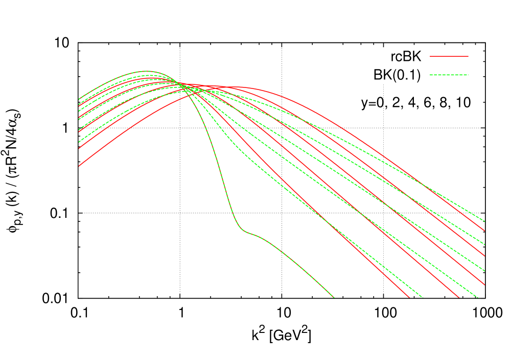
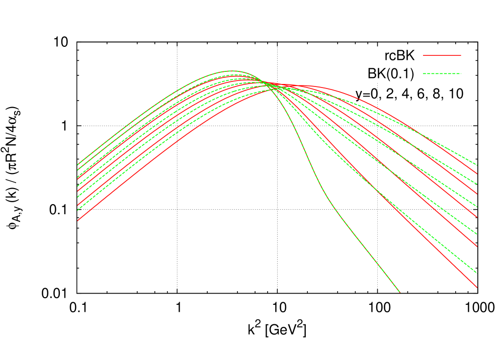
Figure 1: Left: Evolution of the proton uGD, $\phi_{y}(k_{\perp}^{2})/(\pi R^{2}N/4\alpha_{s})$ obtained by solving the rcBK equation (solid) and the BK equation with fixed $\alpha_{s}=0.1$ (dashed) with the initial condition of set g1118. Right: the same with replacing $Q_{s0}^{2}=6Q_{s0,p}^{2}$.

We consider here the $x_{1,2}$ coverage of the charm pair production in the plane of the rapidity $y$ and the transverse momentum $P_{\perp}$ of the pair at collision energies $\sqrt{s}$=200 GeV and 5.02 TeV in Fig. 2. Here we fix the pair’s invariant mass $M=3.1$ GeV, and draw the curves determined by $x_{1,2}=e^{\pm y}(\sqrt{P_{\perp}^{2}+M^{2}}/\sqrt{s})$, on which either $x_{1}$ or $x_{2}$ is constant. The kinematically disallowed region where $x_{1,2}>1$ is indicated by the shaded area. We see that, at the RHIC energy, J/$\psi$ is produced from the gluons of moderate $x_{1,2}\sim 0.01-0.05$ at mid-rapidities, while at forward rapidities $y\sim 2$ the process gets sensitivity to the gluons at small $x_{2}<0.01$. At the LHC energy, on the other hand, J/$\psi$ production is already sensitive to the small $x_{2}$ gluon even at mid-rapidity, and at forward rapidity it probes $x_{2}$ as low as $\sim 10^{-(4-5)}$.

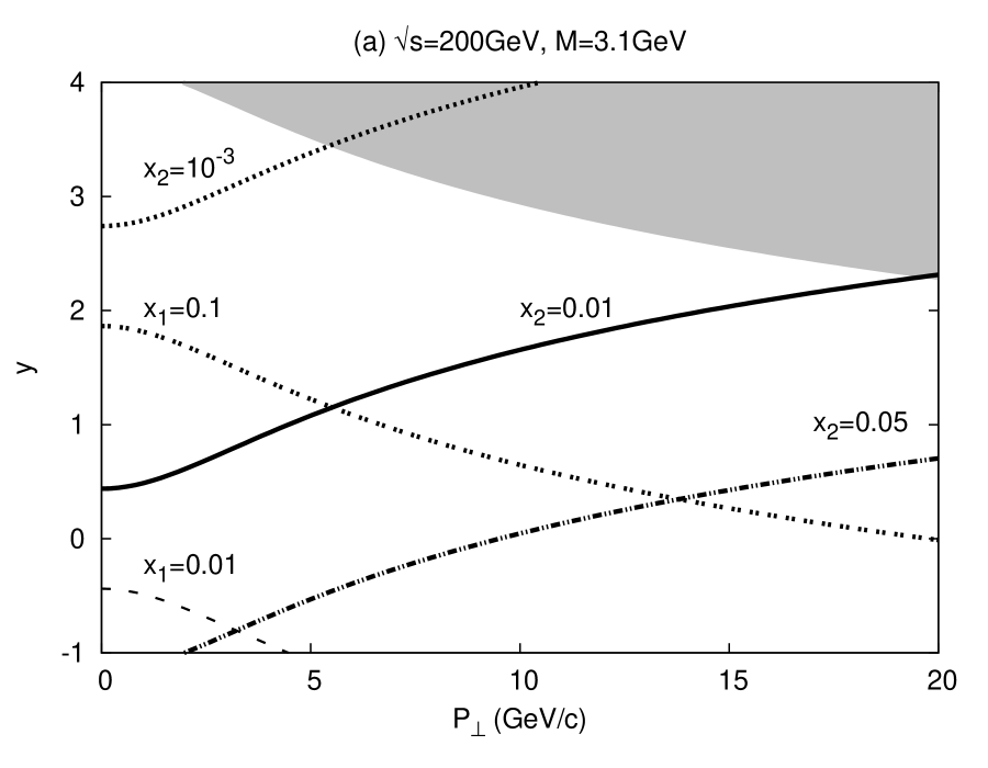
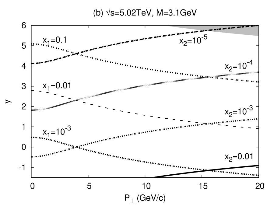
Figure 2: Kinematical coverage of the pair production in the plane of rapidity $y$ and transverse momentum $P_{\perp}$ for invariant mass $M=3.1$ GeV at (a) $\sqrt{s}$=200 GeV and (b) $\sqrt{s}$=5.02 TeV. Shown are the curves of constant $x_{1,2}=(\sqrt{P_{\perp}^{2}+M^{2}}/\sqrt{s})e^{\pm y}$. The shaded region is kinematically forbidden.

In the next section, we study the quarkonium production in CEM applied for the heavy-quark production cross-section (LABEL:eq:cross-section-LN) or (LABEL:eq:cross-section-LN-coll) with the $x$-evolved uGD $\phi_{A,Y}^{q\bar{q},g}({\boldsymbol{k}})$. CEM has been successful in describing the J/$\psi$ production in high-energy proton-proton (pp) collisions.

3 Quarkonium production

We estimate the J/$\psi$ production from the quark-pair production cross section within CEM[15]:

$$\frac{d\sigma_{\text{J}/\psi}}{d^{2}{\boldsymbol{P}}_{\perp}dy}=F_{\text{J}/\psi}\;\int_{4m_{c}^{2}}^{4M_{D}^{2}}dM^{2}\frac{d\sigma_{c\bar{c}}}{d^{2}{\boldsymbol{P}}_{\perp}dM^{2}dy}\,,$$ (24)

where $m_{c}$ ($M_{D}$) is the charm quark ($D$-meson) mass. A phenomenological constant $F_{\text{J}/\psi}$ represents the nonperturbative transition rate for the charm pairs, produced in the invariant mass range from $2m_{c}$ to the threshold $2M_{D}$, to bound into a quarkonium. Its empirical value is around $F_{\text{J}/\psi}=0.01$–0.05[38]. Use of CEM for pA collisions assumes that the bound state formation occurs outside the target nucleus. We fix the threshold with $M_{D}$ ($M_{B}$) = 1.864 (5.280) GeV for J/$\psi$ ($\Upsilon$).

A remark is here in order. In the pair-production cross section (LABEL:eq:cross-section-LN) the inelastic cross section estimated as $\pi R_{\text{A}}^{2}$ in the denominator effectively cancels out with the same factor in $\phi_{A,y}^{q\bar{q},g}$, and that the cross section is now proportional to the effective transverse area $\pi R_{p}^{2}$ of the proton appearing in $\varphi_{p,y}$. In the following calculations, we choose the proton size $R_{\text{p}}=0.9$ fm and the J/$\psi$ formation fraction $F_{\text{J}/\psi}=0.02$ as representative values. One should keep in mind that the absolute normalization of the cross section depends on these parameters. We also cancels $\alpha_{s}$ in front of the cross section by $\alpha_{s}$ appearing in the denominator in $\phi_{A,y}$ and $\varphi_{p,y}$. In the case of collinear approximation on the proton side, we set $\alpha_{s}=0.2$ in this paper.

3.1 Transverse momentum spectrum of J/$\psi$

RHIC

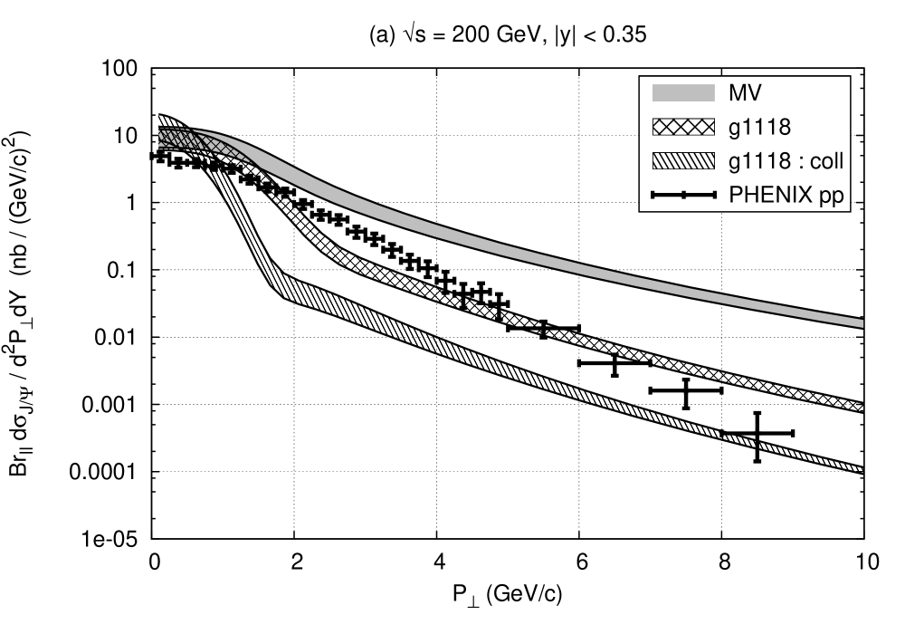
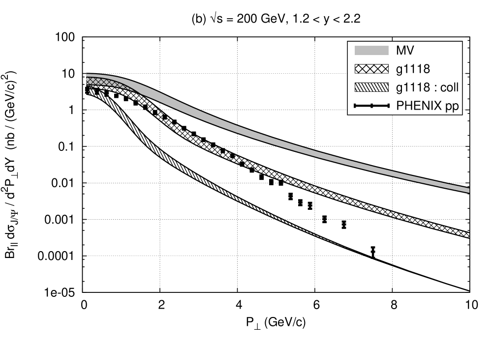
Figure 3: Transverse momentum spectrum of J/$\psi$ in di-lepton channel in pp collisions at $\sqrt{s}=200$ GeV for rapidity ranges (a) $|y|<0.35$ and (b) $1.2<y<2.2$. CEM model results using the pair production (LABEL:eq:cross-section-LN) with sets MV and g1118 are shown in gray and doubly-hatched bands, respectively, and the result using collinear approximation (LABEL:eq:cross-section-LN-coll) with set g1118 is in hatched band. The upper (lower) curve of the band corresponds to the result with $m_{c}=1.2$ (1.5) GeV, and the scale of pdf is chosen at $2M_{\perp}$ ($M_{\perp}/2$) in the collinear approximation. Data from [39].

We first show in Fig. 3 the transverse momentum spectrum of the produced J/$\psi$ in pp collisions at $\sqrt{s}=200$ GeV, using the uGD set g1118 given in Table 1. The upper (lower) curve of each band indicates the result with charm quark mass $m_{c}=1.2$ (1.5) GeV. In the collinear approximation on the larger-$x_{1}$ side, we adopt CTEQ6LO parametrization[40], and the band in Fig. 3 includes the change of the factorization scale from $2M_{\perp}$ to $M_{\perp}/2$ with $M_{\perp}=(M^{2}+P_{\perp}^{2})^{1/2}$, where $M$ is the pair’s invariant mass.

As mentioned above, the quarkonium production at mid-rapidity $|y|<0.35$ is largely determined by the gluon distributions at moderate $x_{1,2}\gtrsim 0.01$. Then, we notice a difficulty with set g1118: the peculiar dip structure of g1118 seen in Fig. 1 remains in the J/$\psi$ spectrum as a similar dip around $P_{\perp}\sim 2$ GeV, which must be an artifact of this initial condition. In contrast, we don’t see such a structure with the MV initial condition. At forward-rapidity $1.2<y<2.2$, the dip is smeared to be less noticeable by the imbalance between $x_{1}$ and $x_{2}$ and by the $x_{2}$ evolution of the uGD. As a whole, the $P_{\perp}$ spectrum obtained with set g1118 is closer to the observed data [39] than with set MV. In this pp case, the collinear approximation on the large-$x_{1}$ side does not improve the description of the data. The $k_{\perp}$ kick from only the one of the protons cannot give enough $P_{\perp}$ for the pair.

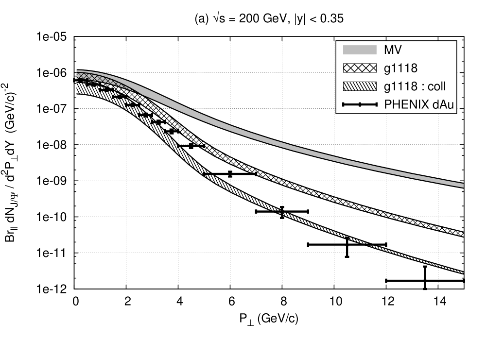
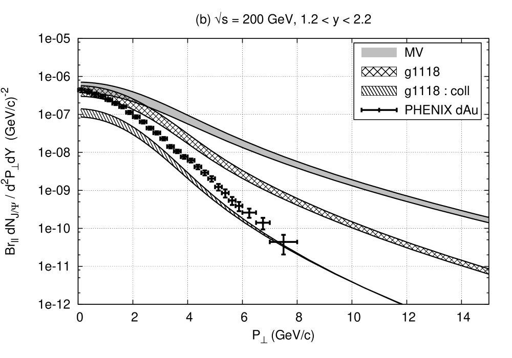
Figure 4: Transverse momentum spectrum of J/$\psi$ in di-lepton channel in pA collisions at $\sqrt{s}=200$ GeV for rapidity ranges (a) $|y|<0.35$ and (b) $1.2<y<2.2$. Notations are the same as in Fig. 3. Data in d-Au collisions[41] are overlaid for comparison.

In Fig. 4 shown is the transverse momentum spectrum of the J/$\psi$ in pA collisions in our model. We set the initial saturation scale of the uGD for the heavy nucleus as $Q_{s0,A}^{2}=6Q_{s0,p}^{2}$ at $x=x_{0}$. The upper (lower) curve of each band indicates the result with $m_{c}=1.2$ (1.5) GeV. We overlay d-Au data observed by PHENIX at $\sqrt{s}=200$ GeV[41], presuming here that the difference between pA and dA results only in normalization difference of order O(1) . We find that $P_{\perp}$-dependence of J/$\psi$ production is better described with set g1118  than that with set MV. Indeed, here the collinear approximation on the proton side apparently gives a better description of the data both at mid- and forward-rapidity regions. However, at forward rapidities, where we approach the small-$x_{2}$ region and the kinematical boundary for $x_{1}$ at the same time (see Fig. 2), we expect a nontrivial interplay between large $x_{1}$ and small $x_{2}$. Besides the saturation dynamics of $x_{2}$ gluons, one may need to consider other physics such as energy loss of large-$x_{1}$ gluons in the heavy target[43] in order to understand the $P_{\perp}$ spectrum of J/$\psi$ in the very forward region. These effects are not included in our present treatment.

We notice in Fig. 4 (b) that the J/$\psi$ production is more suppressed nearly by one order of magnitude in the collinear approximation than those in the full calculation. This is caused by a difference in the large $x_{1}$ behavior of gluon distributions on the proton side. As $x\to 1$, the CTEQ gluon distribution decreases much more rapidly than our model uGD $\varphi_{p,y}$, which is assumed as $\propto(1-x)^{4}$. Furthermore, in the collinear approximation, the pair’s $P_{\perp}$ is entirely provided from the nucleus side, $P_{\perp}=k_{2}$, and uGD $\phi_{A,y}$ for the heavy target is more suppressed at low $k_{2}$ by multiple scatterings.

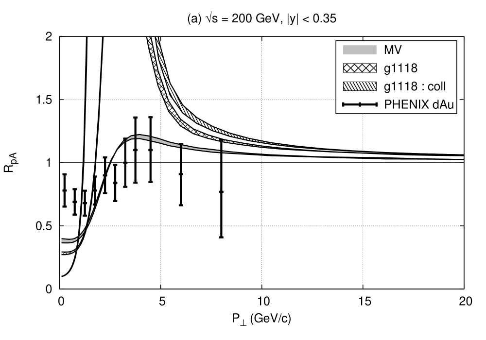
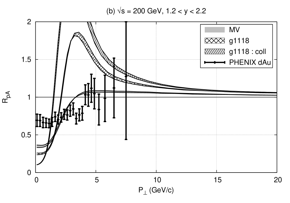
Figure 5: The ratio of J/$\psi$ productions in pA and pp collisions $R_{\text{pA}}(P_{\perp})$ at $\sqrt{s}=200$ GeV for (a) $|y|<0.35$ and (b) $1.2<y<2.2$. The results with uGD sets MV and g1118 are shown in gray and doubly-hatched bands, respectively, and the result in collinear approximation with set g1118 is shown in a hatched band. Notations are the same as in Fig. 3. Data of $R_{dAu}$ taken from [41].

Now let us take a ratio of the cross section of J/$\psi$ in pA collisions to that in pp collisions, which is called nuclear modification factor $R_{\text{pA}}$. We expect that model uncertainties cancel out to some extent in the ratio. We define $R_{\text{pA}}$ for J/$\psi$ in our model as

$$R_{\text{pA}}=\frac{\left.d\sigma_{{\rm J}/\psi}/d^{2}P_{\perp}dy\right|_{\text{pA}}}{N_{\text{coll}}\,\left.d\sigma_{{\rm J}/\psi}/d^{2}P_{\perp}dy\right|_{\text{pp}}}\;.$$ (25)

Here we set the number of nucleon-nucleon collisions in pA to $N_{\text{coll}}=A^{\gamma/3}$ because the uGD $\phi_{A,y_{0}}({\boldsymbol{k}}_{\perp})$ scales as $(Q_{s0}^{2})^{\gamma}\propto A^{\gamma/3}$ at large $k_{\perp}$.

In Fig. 5 we compare the model results for $R_{\text{pA}}$ at $\sqrt{s}=200$ GeV with the data of $R_{\text{dAu}}$. Note that the projectile is different between the model calculation and the data. The notations are the same as in Fig. 3. We stress here that $R_{\rm pA}$ is indeed little dependent on the choice of the quark mass and factorization scale. Unfortunately, however, one immediately recognizes an unphysically strong Cronin peak in the model calculations with set g1118 both at mid- and forward rapidities, which is obviously caused by the dip seen in the pp collisions (Fig. 3). In contrast, the $R_{\rm pA}$ result with set MV looks more reasonable; we see a moderate Cronin peak at mid-rapidity due to the multiple scatterings, while it almost disappears at forward rapidity $y\sim 2$ by the $x_{2}$ evolution. In low-$P_{\perp}$ region, we also notice a too strong suppression than the experimental data. This would imply the importance of the fragmentation process in the formation of J/$\psi$, which is missing in a simple CEM treatment.

To summarize the results at RHIC energy, the J/$\psi$ production spectrum is sensitive to the moderate value of $x_{1,2}$, where the initial condition for the $x$-evolution is set. We have a difficulty to describe the pp data and therefore the ratio $R_{\text{pA}}$ with the uGD g1118 constrained at $x<0.01$. In contrast the set MV gives more reasonable behavior for $R_{\text{pA}}$. In pA collisions the $P_{\perp}$ spectrum is better described with set g1118 at mid- and forward-rapidities. In forward rapidity, the observed $P_{\perp}$ slope is still steeper than the model, hinting other effects such as a possible energy loss of the large-$x_{1}$ gluon from the proton. Actually $R_{\rm dA}$ of J/$\psi$ at RHIC energy has been studied in several approaches (e.g.) with introducing nuclear parton distribution and nuclear absorption effects to a J/$\psi$ production model for pp[42], or with taking account of the multiple scatterings and energy loss of the projectile gluons[43].

LHC

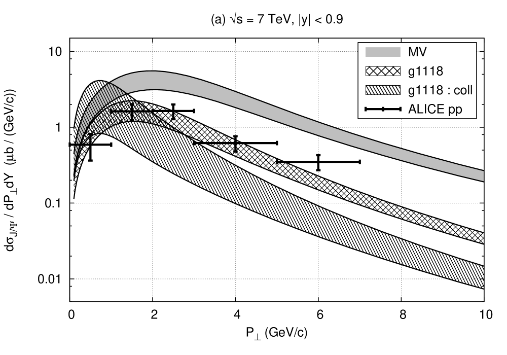
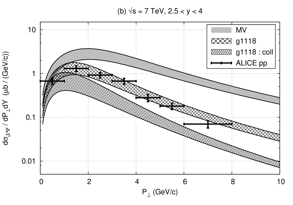
Figure 6: Differential J/$\psi$ yield in pp collisions at $\sqrt{s}=7$ TeV for (a) $|y|<0.9$ and (b) $2.5<y<4$. Notations are the same as in Fig. 3. Data from [44].

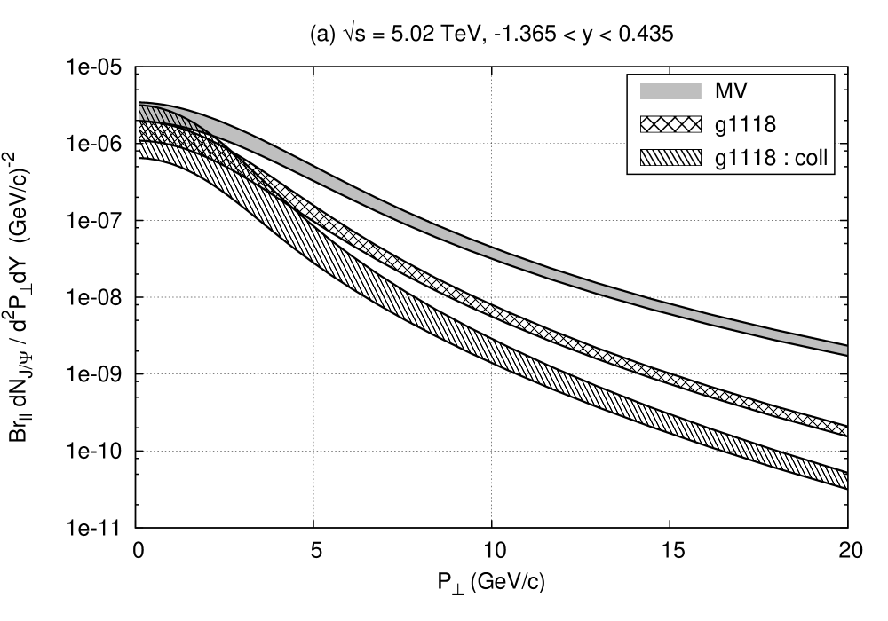
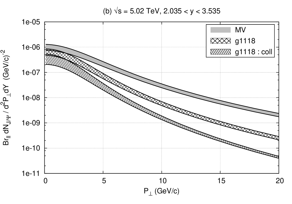
Figure 7: Transverse momentum spectrum of J/$\psi$ in di-lepton channel in pA collisions at $\sqrt{s}=5.02$ TeV for (a) $-1.4<|y|<0.4$ and (b) $2<y<3.5$. Notations are the same as in Fig. 3.

Now we compute the J/$\psi$ production at the LHC energy, where we expect that a wider $x_{2}$-evolution of uGD on the nucleus side will manifest in the quarkonium spectrum. In fact, both $x_{1,2}$ are small ($\sim 10^{-3}<x_{0}$) already in mid-rapidity production of the charm pair as seen in Fig. 2, and as moving to larger rapidities we can probe smaller values of $x_{2}$ on the nucleus side down to $x_{2}\sim 10^{-5}$.

We show in Fig. 6 the J$/\psi$ cross section in pp collision at $\sqrt{s}=7$ TeV, obtained in CEM from charm quark spectrum (LABEL:eq:cross-section-LN). Notations are the same as in the case of the RHIC energy. In order to assess the uncertainty, we again vary the charm quark mass from $m_{c}=1.2$ to 1.5 GeV, and change the factorization scale from $2M_{\perp}$ to $M_{\perp}/2$ in the collinear approximation. The observed data[44] is fairly well reproduced with set g1118 in this $P_{\perp}$ region both at $|y|<0.9$ and $2.5<y<4$, indicating that $y$-dependence is appropriately captured by $x$ evolution of uGD. The $P_{\perp}$ slope in the collinear approximation (LABEL:eq:cross-section-LN-coll) with set g1118 seems to be slightly off the data, while the full result with set MV gives harder $P_{\perp}$ spectrum. The situation is expected to be similar in pp collisions at $\sqrt{s}=5.02$ TeV.

Results in pA collisions at $\sqrt{s}=5.02$ TeV are plotted at mid- and forward-rapidities in Fig. 7. The MV initial condition gives a harder spectrum of J/$\psi$ than g1118. But their $P_{\perp}$ slopes become almost the same at $P_{\perp}\gtrsim 10$ GeV, hinting the same BFKL tail of uGD generated during the evolution. Compared to the case at the lower energy $\sqrt{s}=200$ GeV, the collinear approximation (with set g1118) results in the spectral shape rather similar to the full result at this energy $\sqrt{s}=5.02$ TeV, where the collinear approximation on the proton side would be more suitable since the saturation scale of the nucleus is much larger than that of the proton: $Q_{s,A}^{2}(x_{2})\gg Q_{s,p}^{2}(x_{1})$, especially in the forward region.

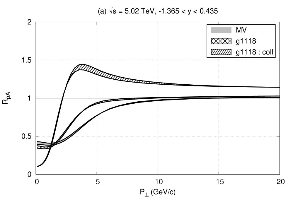
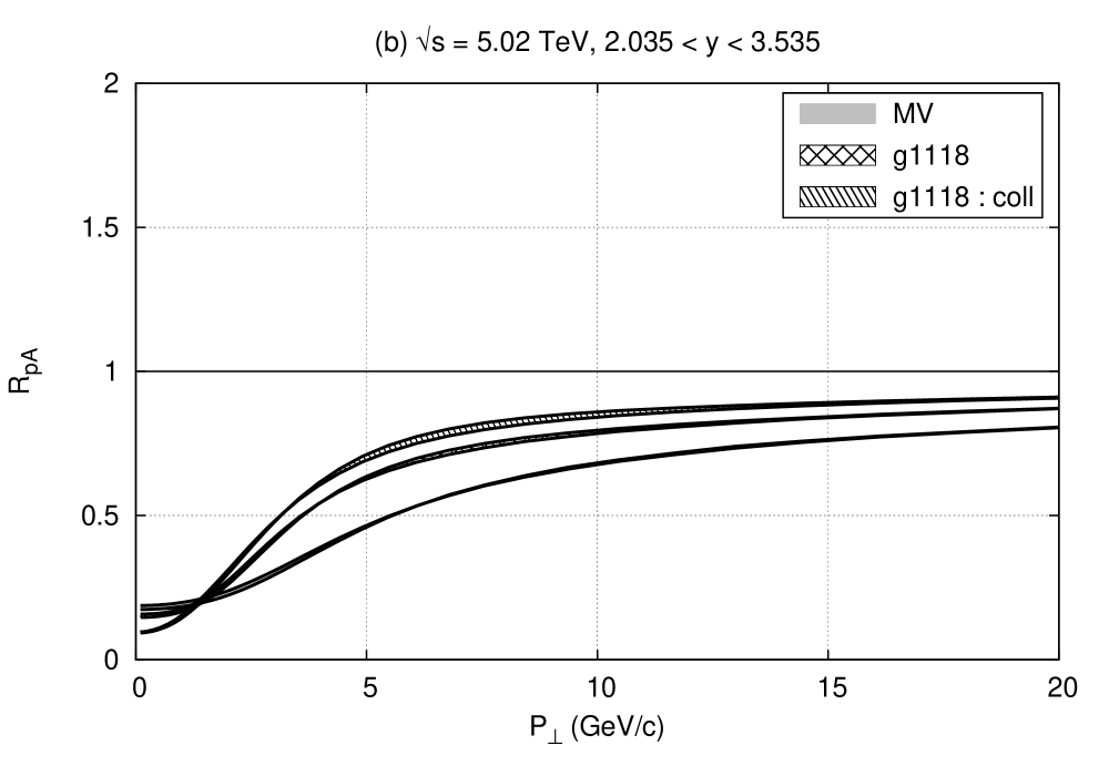
Figure 8: The ratio $R_{\text{pA}}(P_{\perp})$ for J/$\psi$ at $\sqrt{s}=5.02$ TeV for (a) $-1.4<y<0.4$ and (b) $2<y<3.5$. Notations are the same as in Fig. 3.

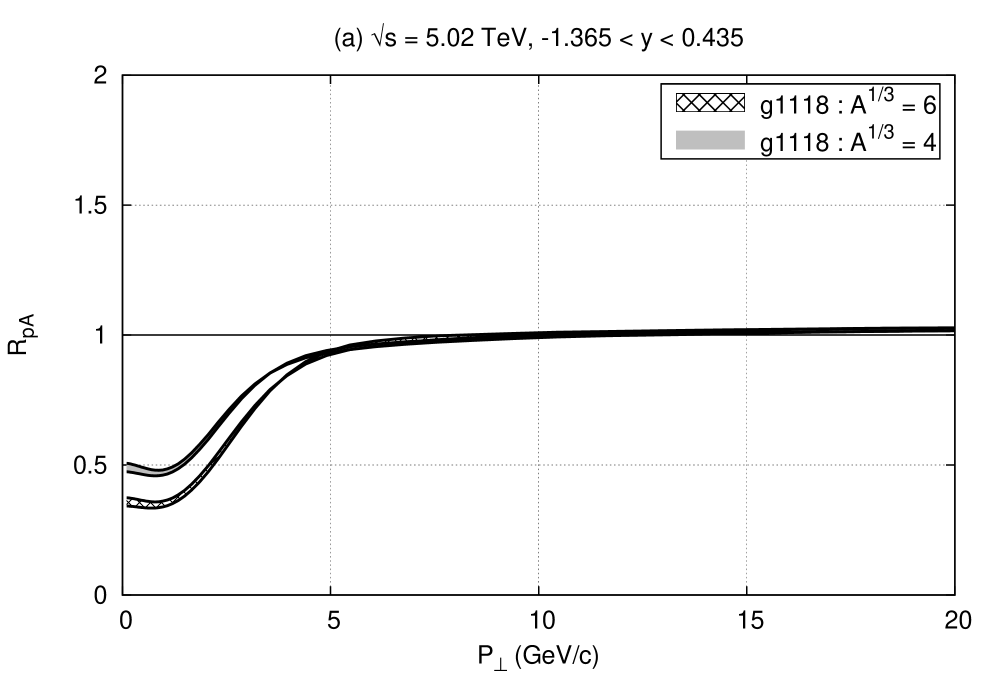
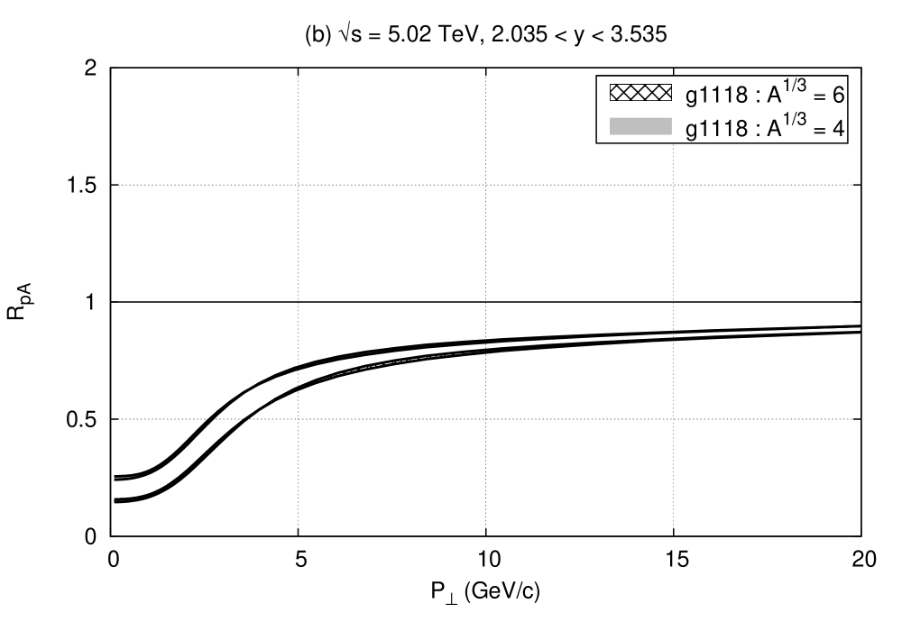
Figure 9: Initial-scale dependence of the ratio $R_{\text{pA}}(P_{\perp})$ for J/$\psi$ at (a) mid- and (b) forward-rapidities at $\sqrt{s}=5.02$ TeV. $Q_{s0,A}^{2}$ is set to $4Q_{s0,p}^{2}$ (upper) and $6Q_{s0,p}^{2}$ (lower).

We show in Fig. 8 the ratio $R_{\text{pA}}$ of J/$\psi$ as a function of $P_{\perp}$ at $\sqrt{s}=5.02$ TeV. We have assumed $N_{\text{coll}}=A^{\gamma/3}$ as mentioned before. We find that each band almost collapses into a single line, which means that the ratio $R_{\text{pA}}$ is insensitive to the variation of the charm quark mass (and the factorization scale in the collinear approximation) within the range considered here.

At mid-rapidities (Fig. 8 (a)), we see that the ratio $R_{\text{pA}}$ of J/$\psi$ production is suppressed at low $P_{\perp}$, while it approaches unity at higher $P_{\perp}$ for both sets of g1118 and MV. In the collinear approximation on the proton side, $R_{\text{pA}}$ shows a Cronin-like peak around $P_{\perp}\sim 4$ GeV and remains larger than unity at larger $P_{\perp}$, which largely reflects “$R_{\text{pA}}$ for $\phi_{A,y}$” at the gluon level. At forward rapidities (Fig. 8 (b)), however, this difference due to different uGD sets and approximations becomes much weaker to yield a systematic suppression as a function of $P_{\perp}$ for all three cases.

We examine the initial-scale ($Q_{s0,A}^{2}$) dependence of the ratio $R_{\text{pA}}$ in Fig. 9, by plotting the results with the saturation scale $Q_{s0,A}^{2}=4Q_{s0,p}^{2}$ (upper) and $6Q_{s0,p}^{2}$ (lower) in Eq. (20) at $x=x_{0}$. It is found that the $Q_{s0,A}^{2}$ dependence of $R_{\text{pA}}$ is relatively weak within this range. At low $P_{\perp}$ we have strong suppression, but one should keep in mind that this suppression may be filled to some extent by the nonperturbative fragmentation in forming J/$\psi$, as is inferred from the discussion on Fig. 5.

To summarize the result at LHC energy, we can probe here a wide $x_{2}$-evolution of the uGD $\phi_{A,y_{2}}({\boldsymbol{k}}_{2})$ through the J/$\psi$ production, and the ratio $R_{\text{pA}}$ will be a good indicator for it.

3.2 $\Upsilon$ production at the LHC

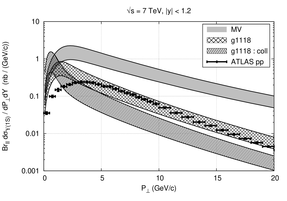
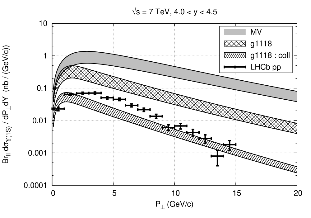
Figure 10: Transverse momentum spectrum of $\Upsilon(1S)$ in di-lepton channel in pp collisions at $\sqrt{s}=7$ TeV for (a) $|y|<1.2$ and (b) $4<y<4.5$. Notations are the same as in Fig. 3. Data from [45, 46].

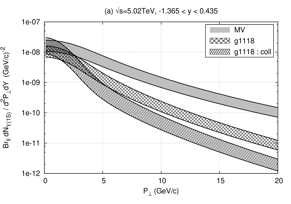
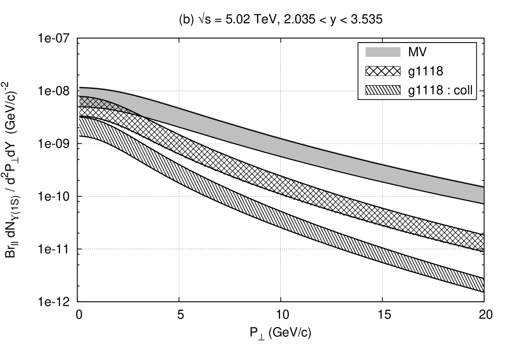
Figure 11: Transverse momentum spectrum of $\Upsilon(1S)$ in di-lepton channel in pA collisions at $\sqrt{s}=5.02$ TeV for (a) $-1.4<y<0.4$ and (b) $2<y<3.5$. Notations are the same as in Fig. 3.

Next we consider $\Upsilon(1S)$ production. Non-linear effects are generally suppressed by the inverse power of the heavy quark mass. However, since the bottom quark mass $m_{b}$ is just three times as heavy as the charm quark mass $m_{c}$, the relevant value of $x$ for the $\Upsilon(1S)$ production becomes larger by the same factor at low $P_{\perp}$, as compared to the J/$\psi$. At the LHC energy, this $x$ value may be still small enough for multiple scatterings and saturation to be relevant in the $\Upsilon$ production.

We plot the $P_{\perp}$ spectrum of $\Upsilon(1S)$ in pp and pA collisions at $\sqrt{s}=7$ and 5.02 TeV, respectively, in Figs. 10 and 11, together with the data measured by ATLAS and LHCb[45, 46] for the pp case. Here we have chosen the CEM parameter as $F_{\Upsilon(1S)}=0.01$, and varied $m_{b}$ from 4.5 to 4.8 GeV. Other notations are the same as in the J/$\psi$ case. In pp collisions, the coincidence between the model and the data for $\Upsilon(1S)$ state is not as good as that for J/$\psi$ at low $P_{\perp}$ and at forward rapidity.

We present in Fig. 12 the nuclear modification factor $R_{\text{pA}}$ for $\Upsilon(1S)$ as a function of $P_{\perp}$. The model uncertainty from the quark mass value and the factorization scale would cancel out by taking the ratio of the cross-sections in the pp and pA collisions. Indeed, each band collapses into a thin line whose width is almost unnoticeable.

This result for $\Upsilon(1S)$ is qualitatively very similar to that for J/$\psi$. At mid-rapidity, we see a suppression $R_{\text{pA}}$ in low $P_{\perp}$ region below 5 GeV, while it turns back to unity at larger $P_{\perp}$. Only in the collinear approximation, we see the Cronin-like enhancement, which is largely caused by the dip structure in the proton uGD at moderate $x_{1}$. At forward rapidities $2<y<3.5$, the $\Upsilon$ production is suppressed in a wide $P_{\perp}$ region from 0 to 20 GeV, irrespective of the model uGD’s, g1118 or MV, or of the use of collinear approximation. In the forward region, $\Upsilon(1S)$ production has the sensitivity to the small-$x$ evolution of uGD in the nucleus.

We have also checked the initial-scale ($Q_{s0,A}^{2}$) dependence of $R_{\text{pA}}$ for $\Upsilon(1S)$ by comparing the result with $Q_{s0,A}^{2}=4Q_{s0,p}^{2}$ and $6Q_{s0,p}^{2}$ to find that the change is very similar to the case with J/$\psi$ (Fig. 9).

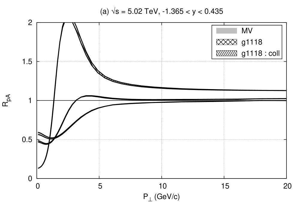
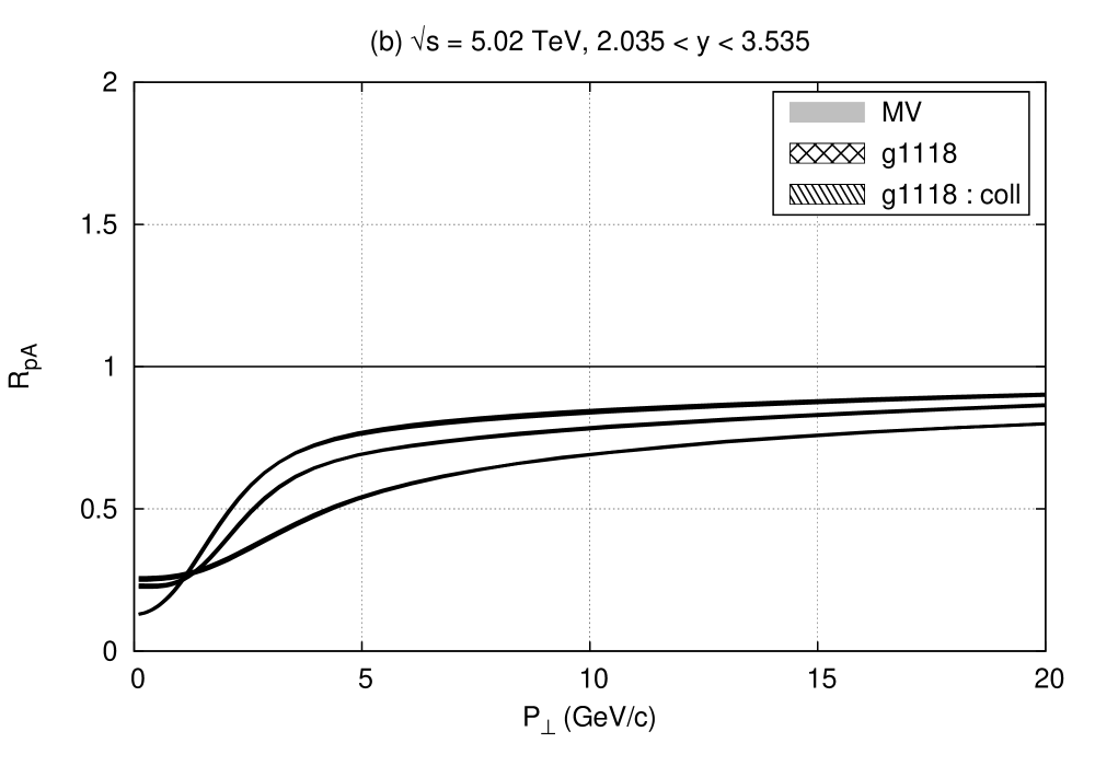
Figure 12: The ratio $R_{\text{pA}}$ for $\Upsilon(1S)$ at $\sqrt{s}=5.02$ TeV as a function of the transverse momentum. (a) $-1.4<y<0.4$ and (b) $2<y<3.5$. Notations are the same as in Fig. 3.

3.3 Rapidity dependence of $R_{\text{pA}}$ of J/$\psi$ and $\Upsilon$

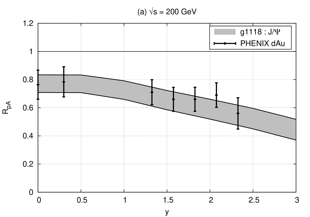
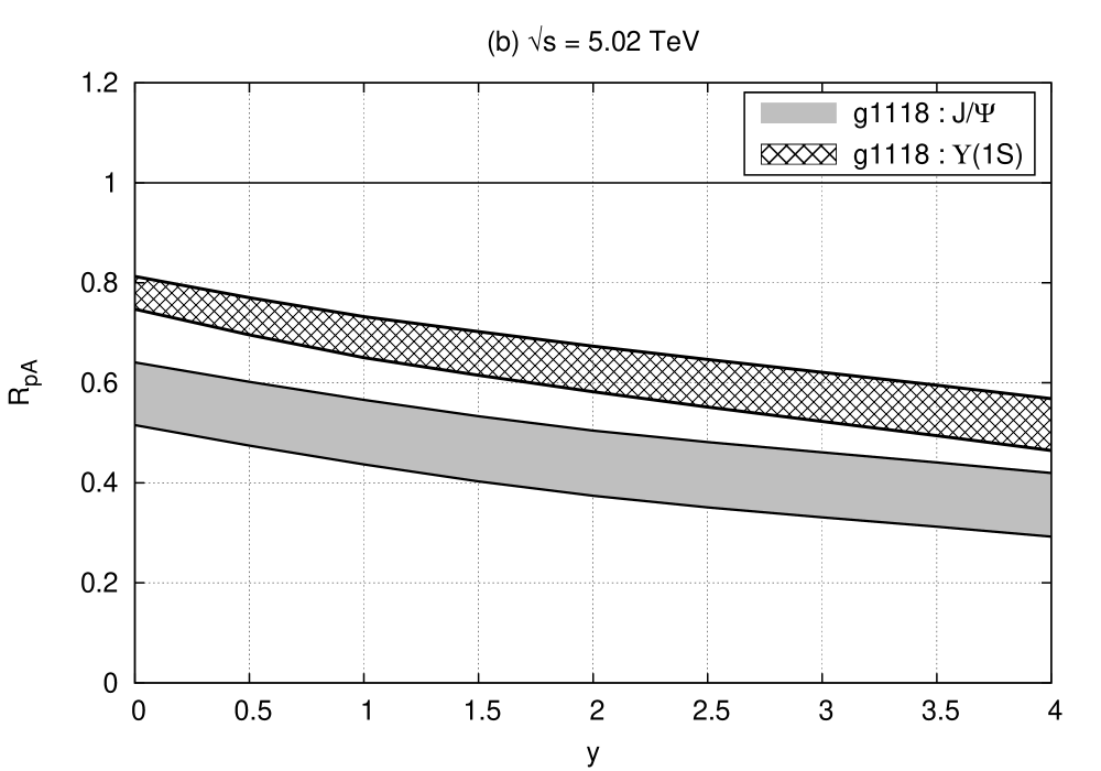
Figure 13: Nuclear modification factor $R_{\text{pA}}$ for J/$\psi$ integrated over $P_{\perp}$ as a function of rapidity, in pA collisions at (a) $\sqrt{s}=200$ GeV and (b) $\sqrt{s}=5.02$ TeV. The band includes uncertainty for $m_{c}=1.2$ GeV to 1.5 GeV and $Q_{s0,A}^{2}=(4-6)Q_{s0,p}^{2}$. In (b), $R_{\text{pA}}$ of $\Upsilon(1S)$ is also shown where we vary $m_{b}=4.5$ to 4.8 GeV. RHIC data from [47].

We study the rapidity dependence of the ratio $R_{\text{pA}}$ integrated over $P_{\perp}$. The computation is performed with set g1118. In Fig. 13 shown is $R_{\text{pA}}(y)$ of J/$\psi$ at $\sqrt{s}=0.2$ and 5.02 TeV, together with that of $\Upsilon(1S)$ for the latter. Note that our assumption of dilute-dense colliding system applies only in the positive rapidity region ($y>0$), especially for pp, which is needed in the denominator of $R_{\text{pA}}$.

We see systematically a stronger suppression of $R_{\text{pA}}$ as the rapidity increases both at RHIC and LHC energies. This is in accord with $x$-evolution of uGD in the heavy target. $R_{\text{pA}}(y)$ of J/$\psi$ flattens out at $y\lesssim 1$ at RHIC energy because the J/$\psi$ is produced there by the gluons with $x_{2}>x_{0}$ and we freeze the saturation scale to its initial value $Q_{s}^{2}(x>x0)=Q_{s,0}^{2}$.

Comparing the results of J/$\psi$ and $\Upsilon(1S)$ at LHC, we note that the suppression of $\Upsilon(1S)$ is smaller than that of J/$\psi$, but is still significant to be observed. It would be quite important to study these systematics in experimental data in order to quantify the saturation effects in the heavy nuclear target.

3.4 $Q_{s0,A}^{2}$ dependence of $R_{\text{pA}}$

It would be interesting to study the dependence of $R_{\text{pA}}$ on the saturation scale parameter $Q_{s0,A}^{2}$, which may be translated to the effective thickness of the target. We compute $R_{\text{pA}}$ of J/$\psi$ and $\Upsilon(1S)$ integrated over $P_{\perp}$ as a function of $Q_{s0,A}^{2}$ at several values of $y$. We fix here the uGD set g1118 and the quark masses as $m_{c}=1.5$ GeV and $m_{b}=4.8$ GeV. In Fig. 14 we plot $R_{\text{pA}}$ of J/$\psi$ at $\sqrt{s}=0.2$ and 5.02 TeV. We found that for each rapidity $Q_{s0,A}^{2}$-dependence of $R_{\text{pA}}$ can be fitted nicely by a model function:

$$R_{\text{pA}}=\frac{a}{(b+Q_{s0,A}^{2})^{\alpha}}$$ (26)

with $a$, $b$ and $\alpha$ being parameters. This functional form is motivated by QCD analog of superpenetration of a electron-positron pair through a medium[48, 11]. We show $\Upsilon(1S)$ result in Fig. 15 with fitted curves. The stronger suppression at the larger value of $Q_{s0,A}^{2}$ is naturally understood as a result of stronger multiple scatterings and saturation effects in the heavier target.

Energy and rapidity dependences may be qualitatively inferred through the increase of $Q_{s,A}^{2}(y)$ with increasing $y$. Thus we tried to fit the rapidity dependence of $R_{\text{pA}}$ by replacing in Eq. (26) $Q_{s0,A}^{2}\to Q_{s0,A}^{2}e^{\lambda y}$ with a free parameter $\lambda$, but it was only unsatisfactory. We remark here that quarkonium suppression due to parton saturation in our treatment is twofold: a relative depletion of the gluon source and multiple scatterings of the quark pair in the target. The latter disturbs the boundstate formation, by increasing the pair’s invariant mass on average in CEM[49]. It appears hard to describe energy and rapidity dependence of the suppression at the same time through a single function $Q_{s,A}^{2}(x)$.

Figure 14: Nuclear modification factor $R_{\text{pA}}$ for J/$\psi$ as a function of $Q_{s0,A}^{2}$ at $y=0,1,2$ and $3$ at $\sqrt{s}=200$ GeV (left) and $\sqrt{s}=5.02$ TeV (right). Fitted curves are also shown.

Figure 15: Nuclear modification factor $R_{\text{pA}}$ for $\Upsilon(1S)$ as a function of $Q_{s}^{2}$ at $y=0,1,2$ and $4$ at $\sqrt{s}=5.02$ TeV.

3.5 $P_{\perp}$ broadening

Figure 16: Mean transverse momentum square $\Delta\langle P^{2}_{\perp}\rangle_{\text{pA}}$ of J/$\psi$ as a function of $Q_{s0,A}^{2}$ at $\sqrt{s}=200$ GeV (left) and $\sqrt{s}=5.02$ TeV (right). Fit with a form $a[(Q_{s0,A}^{2}/Q_{s0,p}^{2})^{\alpha}-1]$ is also shown.

Finally, we study the mean transverse momentum of quarkonium in pA collisions. The momentum broadening in the nuclear target has been discussed in the literature[15]. In our framework, the multiple scatterings of the incident gluon and the produced quark pair in the nuclear target, encoded in $U$ and $\tilde{U}$ terms in Eq. (1) respectively, cause the momentum broadening of the pair. Typical momentum transfer of the multiple scatterings in the nucleus should be characterized by the saturation scale $Q_{s,A}(x_{2})$. We define here the broadening of $P_{\perp}$ as the deviation of the mean transverse momentum squared $\langle P_{\perp}^{2}\rangle$ of J/$\psi$ in pA collisions from that in pp collisions:

$$\Delta\langle P^{2}_{\perp}\rangle_{\text{pA}}\equiv\langle P^{2}_{\perp}\rangle_{\text{pA}}-\langle P^{2}_{\perp}\rangle_{\text{pp}}=\frac{\int d\sigma_{\text{pA}}P_{\perp}^{2}}{\int d\sigma_{\text{pA}}}-\frac{\int d\sigma_{\text{pp}}P_{\perp}^{2}}{\int d\sigma_{\text{pp}}}.$$ (27)

In Fig. 16 we plot $\Delta\langle P_{\perp}^{2}\rangle_{\text{pA}}$ as a function of $Q_{s0,A}^{2}$. We use uGD set g1118 with the quark masses $m_{c}=1.5$ GeV and $m_{b}=4.8$ GeV. We have found that for each rapidity the $Q_{s0,A}^{2}$ dependence of the broadening can be fitted in a simple form:

$$\Delta\langle P^{2}_{\perp}\rangle_{\text{pA}}=a[(Q_{s0,A}^{2}/Q_{s0,p}^{2})^{\alpha}-1]$$ (28)

with $a$ and $\alpha$ being parameters.

At $\sqrt{s}=200$ GeV, the broadening at mid-rapidity is obviously linear in $Q_{s0,A}^{2}$, which indicates the random walk nature of the multiple scatterings in the momentum space. In the forward region, we naively expected an increase of the mean momentum by the stronger scatterings, but actually found the opposite, i.e., a decrease from the mid-rapidity value. We interpret this as the effect of kinematical boundary of $x_{1}$ in the forward region (see Fig. 2).

The measured value of $\Delta\langle P_{\perp}^{2}\rangle_{\text{dA}}$ at RHIC[41] seems to be smaller by a factor of 5 than that in Fig. 16, if we naively translate $Q_{s0,A}^{2}$ to the centrality parameter $N_{\text{coll}}$ evaluated for dAu collisions. This strong broadening originates probably from the fact that our model has too hard $P_{\perp}$ spectrum at RHIC energy. But it is at least consistent with data that $P_{\perp}$ broadening at forward rapidities $\sim 2$ is weaker than that at mid-rapidity $y\sim 0$.

At $\sqrt{s}=5.02$ TeV, a wider phase space opens up and we instead see an increase of the mean momentum of J/$\psi$ as moving to the forward rapidity region. We have checked that $\Delta\langle P_{\perp}^{2}\rangle_{\text{pA}}$ gets back to be smaller at $y=6$ than that of mid-rapidity, just as seen in the case of $\sqrt{s}=200$ GeV. Nonlinear dependence on $Q_{s0,A}^{2}$ may imply the different evolution speed of multiple-scattering strength for different initial values $Q_{s0,A}^{2}$. The result for $\Upsilon(1S)$ in Fig. 17 is similar to the J/$\psi$ case, but interestingly the broadening becomes more remarkable; The heavier bottom quark pair can acquire the larger transverse momentum $P_{\perp}$ in multiple scatterings before going beyond the threshold set on the pair’s invariant mass $M^{2}<4M_{B}^{2}$

Figure 17: Mean transverse momentum square $\Delta\langle P^{2}_{\perp}\rangle_{\text{pA}}$ of $\Upsilon(1S)$ as a function of $Q_{s}^{2}$ at $\sqrt{s}=5.02$TeV. Fit with a form $a[(Q_{s0,A}^{2}/Q_{s0,p}^{2})^{\alpha}-1]$ is also shown.

4 Conclusion and Outlook

Quarkonium production in proton-lead collisions provides us with a good opportunity to study the saturation phenomenon in the incident nucleus thanks to the wide kinetic reach at the LHC. We have computed the J/$\psi$ and $\Upsilon(1S)$ production in pA collision at collider energies within CEM based on the CGC quark pair production, and have discussed sensitivity of the quarkonium observables to the parton saturation in the target nucleus. We have presented the calculations with the uGD set g1118 which is constrained with DIS data at $x<x_{0}=0.01$, with and without the collinear approximation, and the calculations with the model uGD set MV for comparison.

At the RHIC energy $\sqrt{s}=200$ GeV, the J/$\psi$ at mid-rapidity is produced not from the small-$x$ gluons, but from the moderate-$x$ gluons, and the $P_{\perp}$ spectrum in pp collisions is unfortunately sensitive to a unphysical dip structure of the uGD set g1118, which was constrained only for $x<x_{0}$. We need better extrapolation of our framework to $x\gtrsim x_{0}$. In pA collisions, multiple scatterings smear out the dip of the uGD and the $P_{\perp}$ spectrum of J/$\psi$ becomes closer to the observed one in dAu collisions.

At the LHC energy $\sqrt{s}=5.02$ TeV, the small-$x$ gluons dominate the charm production, and we have found that our model with the uGD set g1118 works for J/$\psi$ production in pp collisions both at mid- and forward-rapidities. Then we have shown our model prediction on J/$\psi$ production in pA collisions. The ratio $R_{\text{pA}}(P_{\perp})$ for J/$\psi$ shows a suppression for $P_{\perp}\lesssim 5$ GeV at mid-rapidity due to saturation effects, and it is further suppressed in wider range of $P_{\perp}$ as moving to forward rapidities.

We have also shown that the $\Upsilon(1S)$ production in pA collisions at the LHC has a good sensitivity to the gluon saturation of the nucleus, provided that the effect is smaller than that in the J/$\psi$ case. In our model, when integrated over $P_{\perp}$, the ratio $R_{\text{pA}}(y)$ for $\Upsilon$ at the LHC shows a suppression similar to that of J/$\psi$ at RHIC energy.

Transverse momentum broadening $\Delta\langle P_{\perp}^{2}\rangle$ of the quarkonium shows an increasing behavior as a function of $Q_{s0,A}^{2}$. Because our model gives harder $P_{\perp}$ spectrum than the data, the broadening is likely to be overestimated at RHIC energy in our calculation. However, it is still interesting to notice that at RHIC energy the broadening becomes weaker at forward rapidity than at mid-rapidity due to the kinematical constraint. At LHC energy, on the other hand, we expect the increase of the broadening at forward rapidities because of the larger saturation scale $Q_{s}^{2}(x_{2})$ and wider kinematic coverage of the LHC. Transverse momentum broadening is also investigated recently by taking account of the multiple scatterings in the target in [50].

In conclusion, we have numerically studied the quarkonium production in pA collisions at the RHIC and LHC, within CEM based on the CGC quark-pair production energies, and have quantifies the effects of saturation and multiple scatterings in the target nucleus on the J/$\psi$ and $\Upsilon$ observables. Comparison of our results with experimental data at the LHC must be very important to access the relevance of the saturation physics in the quarkonium production.

In this work we have employed CEM to describe the nonperturbative formation of the quarkonia. In fact, quarkonium formation is one of the challenges in QCD, even in pp collisions, and CEM replaces this just by a probability constant $F_{{\rm J}/\psi}$. Non-relativistic QCD framework has recently been extended to NLO, which improves our understanding of quarkonium production significantly[51, 52]. As a first step in this direction we plan to match the quark-pair production from CGC onto the non-relativistic QCD approach.

We can investigate also the production of open heavy flavor mesons in our framework. Modification of $P_{\perp}$ spectrum and $D\bar{D}$ correlations will also provide very useful information on the saturation in the target nucleus and a good benchmark for the energy loss and collective flow measurements of $D$ and $B$ mesons. We will report this elsewhere[53].

References

- [1] F. Gelis, E. Iancu, J. Jalilian-Marian and Raju Venugopalan, Ann. Rev. Nucl. Part. Sci. 60, 463-489 (2010) [arXiv:1002.0333 [hep-ph]], and references therein.
- [2] L. McLerran, R. Venugopalan, Phys. Rev. D 49, 2233; 3352 (1994); D 50 2225 (1994).
- [3] B. Abelev et al. (ALICE Collaboration), Phys. Rev. Lett. 110, 032301 (2013) [arXiv:1210.3615 [nucl-ex]]; 082302 (2013) [arXiv:1210.4520 [nucl-ex]].
- [4] S. Chatrchyan et al. (CMS Collaboration), Phys. Lett. B 718, 795 (2013) [arXiv:1210.5482 [nucl-ex]].
- [5] B. Abelev et al. (ALICE Collaboration), Phys. Lett. B 719, 29 (2013) [arXiv:1212.2001 [nucl-ex]].
- [6] A.M. Stasto, K. Golec-Biernat, J. Kwiecinski, Phys. Rev. Lett. 86, 596 (2001).
- [7] F. Gelis, R. Peschanski, G. Soyez, L. Schoeffel, Phys. Lett. B 647, 376 (2007).
- [8] D. Kharzeev, K. Tuchin, Nucl. Phys. A 735, 248 (2004).
- [9] D. Kharzeev, K. Tuchin, Nucl. Phys. A 770, 40 (2006).
- [10] H. Fujii, F. Gelis, R. Venugopalan, Phys. Rev. Lett. 95, 162002 (2005).
- [11] H. Fujii, F. Gelis, R. Venugopalan, Nucl. Phys. A 780, 146 (2006).
- [12] F. Dominguez, D.E. Kharzeev, E.M. Levin, A.H. Mueller and K. Tuchin, Phys. Lett. B 710 182 (2012).
- [13] D.E. Kharzeev, E.M. Levin and K. Tuchin, arXiv:1205.1554 [hep-ph].
- [14] M. Bedjidian et al., CERN Yellow Report on “Hard Probes in Heavy Ion Collisions at the LHC: heavy flavor physics” [hep-ph/0311048].
- [15] N. Brambilla et al. (Quarkonium Working Group), hep-ph/0412158; Z. Conesa del Valle et al., Nucl. Phys. Proc. Suppl. 214, 3 (2011) [arXiv:1105.4545 [hep-ph]] and references therein.
- [16] T. Matsui, H. Satz, Phys. Lett. B 178, 416 (1986).
- [17] R.L. Thews, M. Schroedter and J. Rafelski, Phys. Rev. C 63, 054905 (2001).
- [18] P. Braun-Munzinger and J. Stachel, Nucl. Phys. A 690, 119 (2001).
- [19] Y.L. Dokshitzer and D.E. Kharzeev, Phys. Lett. B 519, 199 (2001).
- [20] M. Djordjevic and M. Gyulassy, Nucl. Phys. A 733, 265 (2004).
- [21] N. Armesto, M. Cacciari, A. Dainese, C.A. Salgado and U.A. Wiedemann, Phys. Lett. B 637, 362 (2006).
- [22] H. van Hees and R. Rapp, Phys. Rev. C 71, 034907 (2005).
- [23] J.P. Blaizot, F. Gelis, R. Venugopalan, Nucl. Phys. A 743, 13 (2004).
- [24] J.P. Blaizot, F. Gelis, R. Venugopalan, Nucl. Phys. A 743, 57 (2004).
- [25] J.L. Albacete, Yuri V. Kovchegov, Phys. Rev. D 75, 125021 (2007) [arXiv:0704.0612 [hep-ph]].
- [26] J.L. Albacete, Nestor Armesto, J.G. Milhano, C.A. Salgado, Phys. Rev. D 80, 034031 (2009) [arXiv:0902.1112 [hep-ph]].
- [27] J.L. Albacete, N. Armesto, J.G. Milhano, P. Quiroga-Arias, and C.A. Salgado, Eur. Phys. J. C 71, 1705 (2011) [arXiv:1012.4408 [hep-ph]].
- [28] J.L. ALbacete and A. Dumitru, arXiv:1011.5161 [hep-ph].
- [29] J.L. Albacete, A. Dumitru, H. Fujii and Y. Nara, Nucl. Phys. A 897, 1 (2013) [arXiv:1209.2001 [hep-ph]].
- [30] A. Dumitru, A. Hayashigaki, J. Jalilian-Marian, Nucl. Phys. A 765, 464 (2006).
- [31] I. Balitsky, Nucl. Phys. B 463, 99 (1996).
- [32] Yu.V. Kovchegov, Phys. Rev. D 54, 5463 (1996).
- [33] D.N. Triantafyllopoulos, Nucl. Phys. B 648, 293 (2003).
- [34] J.L. Albacete, Phys. Rev. Lett. 99, 262301 (2007) [arXiv:0707.2545 [hep-ph]].
- [35] I. Balitsky, Phys. Rev. D 75, 014001 (2007).
- [36] A. Dumitru and E. Petreska, Nucl.Phys. A 879, 59 (2012) [arXiv:1112.4760 [hep-ph]].
- [37] F. Gelis, A.M. Stasto, R. Venugopalan, Eur. Phys. J. C 48, 489 (2006).
- [38] F. Arleo, et al, CERN Yellow Report on “Hard Probes in Heavy Ion Collisions at the LHC: photon physics” [hep-ph/0311131].
- [39] A. Adare et al., (PHENIX collaboration), Phys. Rev. D 85, 092004 (2012) [arXiv:1105.1966 [hep-ex]].
- [40] J. Pumplin et al. (CTEQ Collaboration), JHEP 0207 012 (2002).
- [41] A. Adare et al. (PHENIX Collaboration), arXiv:1204.0777 [nucl-ex].
- [42] E.G. Ferreiro, F. Fleuret, J.P. Lansberg and A. Rakotozafindrabe, Phys. Lett. B 680, 50 (2009); E.G. Ferreiro, F. Fleuret, J.P. Lansberg, N. Matagne and A. Rakotozafindrabe, Few Body Syst. 53, 27 (2012).
- [43] F. Arleo and S. Peigne, arXiv:1212.0434 [hep-ph]; F. Arleo, R. Kolevatov, S. Peigné, M. Rustamova, arXiv:1304.0901 [hep-ph].
- [44] K. Aamodt et al. (ALICE Collaboration), Phys. Lett. B 704, 442 (2011) [arXiv:1105.0380 [hep-ex]].
- [45] G. Aad et al. (ATLAS Collaboration), Phys. Rev. D 87, 052004 (2013) [arXiv:1211.7255 [hep-ex]].
- [46] R. Aaij et al. (LHCb Collaboration), Eur. Phys. J. C 72, 2025 (2012) [arXiv:1202.6579 [hep-ex]].
- [47] A. Adare et al. (PHENIX Collaboration), Phys. Rev. Lett. 107, 142301 (2011) [arXiv:1010.1246 [nucl-ex]].
- [48] H. Fujii and T. Matsui, Phys. Lett. B 545, 82 (2002); H. Fujii, Nucl. Phys. A 709, 236 (2002).
- [49] H. Fujii, Phys. Rev. C 67 031901 (2003).
- [50] Z. Kang and J.W. Qiu, Phys. Lett. B 721, 277 (2013) [arXiv:1212.6541 [hep-ph]].
- [51] Y.-Q. Ma, K. Wang and K.-T. Chao, Phys. Rev. Lett. 106, 042002 (2011).
- [52] M. Butenschön and B.A. Kniehl, Phys. Rev. Lett. 106, 022003 (2011).
- [53] H. Fujii and K. Watanabe, in preparation.