Crossover from Bosonic to Fermionic features in Composite Boson Systems

Abstract

We study the quantum dynamics of conversion of composite bosons into fermionic fragment species with increasing densities of bound fermion pairs using the open quantum system approach. The Hilbert space of $N$-state-functions is decomposed into a composite boson subspace and an orthogonal fragment subspace of quasi-free fermions that enlarges as the composite boson constituents deviate from ideal boson commutation relations. The tunneling dynamics of coupled composite boson states in confined systems is examined, and the appearance of exceptional points under experimentally testable conditions (densities, lattice temperatures) is highlighted. The theory is extended to examine the energy transfer between macroscopically coherent systems such as multichromophoric macromolecules (MCMMs) in photosynthetic light harvesting complexes.

I Introduction

Composite quasi-particle systems such as excitons (coherent superpositions of electrons and holes) display phase-space filling effects when the mean separation between particles becomes comparable to the exciton Bohr radius. This arises due to the Pauli blocking imam ; thilapauli of scattered fermionic particles which constitute “cobosons” comb07 ; comb08 or composite bosons. The difference between composite bosons and elementary bosons can be seen for instance, in the invariance of Pauli scattering during exchanges between specific fermionic species that can be correlated via several routes comb08 . Such interactions are non-existent in a collection of ideal bosons with negligible overlap, spin and internal structure. Unlike the conventional commutation relations satisfied by ideal boson operators of bound fermion pairs, composite bosons systems obey a series of commutation relations comb10 ; comb11a that are reflective of the underlying fermionic structure of the constituent particles. The excitonic polariton deng ; lauss is one such example of a composite boson system in which the influence of the composite-particle effect on many-body physics can be studied. When the dimensions of quantum dot excitonic polaritons are decreased, anti-bunching features appear. The system undergoes a crossover from bosonic to fermionic display in optical features, characterized by a shift from the Rabi doublet to a Mollow triplet in the optical spectrum lauss . In other systems, the deviations from the ideal boson features may influence the magneto-association of atoms into molecules via Feshbach resonances exptfe1 ; exptfe2 .

Recently, several studies have focussed on the links between the composite particle nature of bosons and entanglement effects Law ; woot ; avancini using the principles of quantum information theory. It was shown that effects of the Pauli exclusion principle diminish when entanglement features dominates Law ; woot ; Sancho ; Rama ; Gavrilik . Measures such as purity $P$ woot ; Tichy have been proposed to quantify the strength of entanglement between the constituent fermions. While the exclusion principle imposes the requirement that an antisymmetric state vector be assigned to an identical group of fermions, the rules becomes less stringent when the fermions become entangled and lose their fermion identity. The exact association between entanglement and the exclusion principle is not well understood as the latter implicates some degree of nonlocal interactions for fermionic particles of the same state to display anti-bunching behavior. Beyond a critical dimension, the tendency of similar fermions to “avoid” each other is lost, with the problem very much dependent on the system parameters such as dimensions and thermodynamic factors. Currently, very few details exists on the nature of the quantum correlation (whether classical or non-classical) that underpins the action of the exclusion principle in composite boson systems.

In this work, we examine the conversion of composite bosons to orthogonal fermionic fragment states due to dominance of Pauli exclusion at increasing densities of the correlated boson system. The specific case of excitons is considered, and the ionic conversion of ${\rm e-h}$ $\to X$ is examined as an equivalent of the well known excitonic Mott transition where the excitonic system ionizes due to space filling effects mott ; zimm at high densities, resulting in a free electron-hole plasma $X$. The situation in which the bound exciton state vanishes and merges into a continuum of scattered states can also be considered as the Mott transition. In this case, the scattered states exist as quasi-free fermions. In a recent study semkat , the Mott effect was noted to occur when the excitonic Bohr radius became nearly the same as the screening length, that is, the bound electron-hole pair states co-existed with the high-density electron-hole liquid phase. While the interplay of several many-body effects are responsible for the Mott transition, questions remain as to whether the conversion from the excitonic state to fermionic plasma-like phase proceeds in a continuous manner.

Different timescales can be seen to operate in the composite boson-fermion system: the highly entangled elementary bosons which operate at fast times compared to the scattering times specific to fermionic species. To this end, the composite bosons can be analyzed via the open quantum system approach based on the system-plus-reservoir model. The total Hilbert space is divided into subsystems according to different timescales and/or states which exist in distinct phases. The Fock-Hilbert space of state vectors associated with a system of identical bosons (fermions) is spanned by only symmetric (antisymmetric) functions. The completeness theorem gross applies to many-particle state vectors in distinct Fock-Hilbert subspaces of antisymmetric and symmetric particle functions. However fluctuation in the number of interacting particles occur when energy dissipates from one subspaces to another. In this work, we consider that the Hilbert space of state-functions is decomposed into a composite boson subspace and an orthogonal fragment subspace of quasi-free fermions. The latter subspace enlarges as the composite boson constituents deviate from ideal boson commutation relations due to enhanced fermionic features. The quantum master equation approach of the Lindblad form lind ; gor may be used to investigate composite boson systems, however evaluation of the density matrix of such high dimensional systems will present insurmountable challenges. Stochastic formalisms such as the quantum trajectory method carmi ; molmer involving non-Hermitian terms which cause quantum jumps, coupled with the Feshbach projection-operator partitioning technique fesh may provide a viable route to study the dynamics of composite bosons. In this study, we employ the Green’s function formalism lipp ; suna to examine the dynamics of composite boson systems.

A coupled system of boson condensate and fragment states with variable fermionic character has implications in the field of quantum information and processing. Composite bosons can be studied in the context of quantum tunneling of macroscopically coherent systems such as the double-well Bose-Einstein condensate. The double-well condensate is a well-known lattice system capable of variable controls ng ; greiner , exhibiting a range of quantum effects such as self-trapping, Josephson oscillations oscil , and entanglement bose ; entr . In this work, we report on oscillations that occur in the coupled composite boson system, with testable predictions based on the quantum dot excitonic systems. These results are extended to analyze multichromophoric macromolecules (MCMMs) in photosynthetic light harvesting complexes. MCMMs are systems of great interest adolp ; flem ; silbey ; recom ; thilhs1 due to the appearance of long-lived quantum coherences, even at physiological temperatures.

This paper is organized as follows. In Section II we provide a brief review of cobosons or composite boson states and their Schmidt decomposition properties, along with description of the Schmidt number and purity measures. The occurrence of the fermionic fragment state which lies orthogonal to the composite boson is highlighted. In Section III, a description of other alternative measures of deviations from ideal boson characteristics is provided, and numerical estimates of the bosonic deviation measure in quantum dots of varying size and fermion pair number is provided. In Section IV, we introduce the open quantum system model and master equation for the exciton-fermion system. The importance of Non-Markovian dynamics due to the fermionic background is briefly described in this Section. In Section V, the tensor structure of the many particle Fock-Hilbert space is examined for the $N$ excitonic bosons, and the tunneling dynamics of composite bosons states is numerically examined using the decay branching ratio in Section VI. A discussion of the appearance of exceptional points under experimentally testable conditions is included as well. In Section VII, we examine the application of results obtained in Section VI to pigment protein complexes in light-harvesting systems, and present our conclusions in Section VIII.

II Schmidt decomposition of Cobosons or composite boson states

Following earlier formalisms of cobosons comprising two fermions Law ; woot ; Combescot2011 , the coboson creation operator of distinguishable fermions in the Schmidt decomposition involving a single index is written as

$$B^{\dagger}=\sum_{j=1}^{J}\sqrt{\lambda_{j}}\;a_{j}^{\dagger}b_{j}^{\dagger},$$ (1)

where $\lambda_{j}$ are the Schmidt coefficients. $a^{\dagger}_{j}$ and $b^{\dagger}_{j}$ are different fermion creation operators in the Schmidt mode $j$, and $J$ denotes the number of Schmidt coefficients schm . The distribution of $\lambda_{j}$ is linked to a measure of entanglement, which is provided via the Schmidt number Law

$${\cal K}\equiv 1/\sum\limits_{j=0}^{\infty}{\lambda_{j}^{2}}$$ (2)

The Schmidt number ${\cal K}$ is the quantum counterpart to the classical Pearson correlation coefficient, and is an important entanglement measure ter ; san where large ${\cal K}$ indicates high correlations and entanglement. ${\cal K}$ is also linked to another quantity known as the purity $P$ woot via $P$=$\frac{1}{\cal K}$, and varies between zero and one. In the case of two particles, $P=\hbox{Tr}\;\rho^{2}$, where $\rho$ is the density matrix of the examined particle.

For two identical particles, (fermions or bosons), the symmetrization postulate constraints a boson (fermion) state associated with the system to be totally symmetric (antisymmetric) under permutation of the particles. As a consequence, the Schmidt decomposition of the state involves more than one term, and a bipartite state of two indistinguishable particles is generally considered entangled. This highlights the importance of the Schmidt number in determining entanglement in quantum states of identical particles ghir . $B$ and $B^{\dagger}$ obey the non-bosonic commutation relation, $[B,B^{\dagger}]=1+s\Lambda$, where $s=+1(-1)$ if the two interacting particles are bosons (fermions), and $\Lambda=\sum\limits_{j=0}^{\infty}{\lambda_{j}}\left({a_{j}^{{\dagger}}a_{j}+b_{j}^{{\dagger}}b_{j}}\right)$. The state of $N$ composite bosons appear as

$$|N\rangle=\frac{1}{\sqrt{\chi_{N}}}\frac{\left(B^{\dagger}\right)^{N}}{\sqrt{N!}}|0\rangle,$$ (3)

where deviations from the ideal boson characteristics are contained in the normalization term $\chi_{N}$ obtained using $\langle N|N\rangle$=1. The effectiveness of the operator $B$ as a bosonic annihilation operator can be seen via the action of operator $B$ on state $|N\rangle$ Law

$$B|N\rangle=\alpha_{N}\sqrt{N}|N-1\rangle+|\mathcal{F}_{N}\rangle,$$ (4)

where $\alpha_{N}$ is a ideality parameter and $|\mathcal{F}_{N}\rangle$ is the fragment state resulting from the non-ideal nature of $|N\rangle$. $\alpha_{N}=\sqrt{\frac{{\chi_{N}}}{{\chi_{N-1}}}}$, which in the case of an ideal composite boson yields the normalization ratio $\chi_{N\pm 1}/\chi_{N}\to 1$. This ratio is seen as a measure of the degree of ideal bosonization for a state of $N$ cobosons, and appears in the pair number mean value corresponding to the state $|N\rangle$ as

$$\langle\hat{N}\rangle=\frac{\langle N|\hat{N}|N\rangle}{\langle N|N\rangle}{=}1{+}(N{-}1)\frac{\chi_{N{+}1}}{\chi_{N}}$$ (5)

and also in the commutator mean Law ,

$$\langle N|[B,B^{\dagger}]|N\rangle=2\frac{\chi_{N+1}}{\chi_{N}}-1$$ (6)

A neat inequality involving the upper and a lower bound to the normalization ratio was determined as $1-P\cdot N\leq\frac{\chi_{N+1}}{\chi_{N}}\leq 1-P$ woot .

The fragment states, $|\mathcal{F}_{N}\rangle$ remain orthogonal to $|N-1\rangle$, yielding the correction factor Law ; Combescot2011

$$\langle\mathcal{F}_{N}|{\mathcal{F}_{N}}\rangle=1-\frac{\chi_{N+1}}{\chi_{N}}-N\left(\frac{\chi_{N}}{\chi_{N-1}}-\frac{\chi_{N+1}}{\chi_{N}}\right).$$ (7)

The ratio $\chi_{N+1}/\chi_{N}$ is strictly non-increasing as $N$ increases woot , and for small bosonic deviations such that $\chi_{N+1}/\chi_{N}\approx 1-\delta$, the last term in Eq. (7) can be dropped, $\langle\mathcal{F}_{N}|\mathcal{F}_{N}\rangle$= $\delta$ and the commutator mean, $\langle N|[B,B^{\dagger}]|N\rangle$ = $1-2\delta$. In the limits, $\alpha_{N}\to 1$, $\delta\to 0$, $\langle\mathcal{F}_{N}|\mathcal{F}_{N}\rangle\to 0$. The formation of the fermionic fragment can be compared to the formation of an electron-hole plasma when the density of a collection of correlated electron-hole is increased, giving rise to an enhancement in fermionic features. With increasing closeness of interacting paired fermions, the electron-holes pairs become unbound as is the case when lattice temperature is also increased. The state of $N$ composite bosons (see Eqs. (3)) with a well-defined atom number evolves into a mixture of lower number states and fragment state $|\mathcal{F}_{N}\rangle$, characterized by the fidelity decay, $\gamma$. The role of $\gamma$ is significant, due to its influence in a Zeno-like mechanism where repeated measurements halts further decay of the composite boson states.

III Alternative measures of deviations from ideal boson characteristics

Here we consider other measures that can be used in place of the purity $P$. An experimentally accessible measure that can be used to capture deviations from ideal boson characteristics is based on the (normalised) second order correlator $g_{2}$ glaub ; glaz , which characterizes the probability of detecting of particles at times $t$ and $t+\tau$

$$g_{2}(\tau)=\frac{\langle{B^{\dagger}}(t){B^{\dagger}}(t+\tau)B(t+\tau)B(t)\rangle}{\langle\hat{N}(t)\rangle\langle\hat{N}(t+\tau)\rangle}$$ (8)

$g_{2}(\tau)$ is based on correlations of the boson operators where $\hat{N}$ is the number operator, $\hat{N}|n\rangle=n|N\rangle$ associated with $N$ fermion pairs. At zero delay,

$$g_{2}(0)=\frac{\langle N_{0}(t)(N_{0}(t)-1)\rangle}{\langle N\rangle^{2}}$$ (9)

where $\langle N_{0}(t)\rangle$ =$\langle{B^{\dagger}}(t)B(t)\rangle$. The second-order correlator provides information on the underlying statistical features, such as the Poissonian case ($g_{2}(0)=1$) in coherent systems involving a large number of Fock states. The anti-bunching , sub-Poissonian case ($g_{2}(0)<1$) is applicable in the fermionic limit at high densities. The classically accessible thermal states which display a bunched, super-Poissonian distribution gives rise to $g_{2}(0)>1$, we do not consider such states in the work here. A simple form of the zero-delay $\tau=0$ correlations for the single-mode state, was obtained as $g_{2}(0)=\frac{\alpha_{N-1}^{2}\alpha_{N}^{2}}{N^{2}}$ lauss , where $\alpha_{N}=\sqrt{N}\sqrt{1-2(N-1)(\frac{a_{\mathrm{B}}}{L})^{2}}$. The latter expression is applicable to excitons of bohr radius $a_{\mathrm{B}}$ in quantum dots of size $L$ at small values of $\frac{a_{\mathrm{B}}}{L}$ and $n\ll\frac{L}{a_{\mathrm{B}}}$. In the pure bosonic case, $g_{2}(0)=(N-1)/N\rightarrow 1$ as $N\rightarrow\infty$. The fermionic structure of excitons becomes noticeable with decrease in $g_{2}(0)$, here we estimate the bosonic deviations using $\delta$ = $1-g_{2}(0)$. Results displayed on Fig. 1 show the increase in the bosonic deviation measure $\delta$ with increase in number density (or decrease in quantum dot size) as quantified by the ratio, $\frac{a_{\mathrm{B}}}{L}$. These results translates to the growth of overlap in fragment states, $\langle\mathcal{F}_{N}|\mathcal{F}_{N}\rangle$=$\delta$ with increase in $\frac{a_{\mathrm{B}}}{L}$.

Figure 1: Bosonic deviation measure $\delta$ as function of fermion pair number $N$ in quantum dots at varying ratios, $\frac{L}{a_{\mathrm{B}}}$= 0.01 (Dark solid line), 0.03 (Blue), 0.05 (Red), 0.07 (Green)

An alternative measure of the bosonic deviations is obtained using the degree of binding of the paired fermions

$$\alpha_{d}=1-\frac{E_{c}}{E_{b}}$$ (10)

where $E_{b}$ is the maximized binding energy of the composite boson, and $E_{c}$ is the smaller binding energy of the quasi-bound fermion pairs, which reaches zero for free fermions. This definition is intimately linked to the distinguishability of paired fermions, a system of many strongly bound fermion pair is less distinguishable and more entangled than one of free fermion species. In the case of excitons in semiconductors at varying temperatures and densities, a mixed phase of bound excitons and free electron hole plasma is formed. Here the degree of ionization of the electron hole plasma, $\alpha_{i}=1-\frac{n_{b}}{n_{f}}$, is a suitable candidate for gauging the bosonic deviations of the excitonic system. The term $n_{b}$ denotes the excitonic density and $n_{f}$ denotes the density of the free electrons or holes at a given temperature and density. The evaluation of $\alpha_{i}$ requires carrier density parameters such as the chemical potentials of distinct species, temperature, band multiplicity, spin degeneracy and an integrand with the retarded Green s function of carriers semkat .

Yet another quantity that provides a measure of deviations from ideal boson characteristics is the $N$-particle non-escape probability in which $N$ paired fermions are found within the same region, $\Sigma$

$$P_{N}(t)=\int_{\Sigma}\prod_{n=1}^{N}dr_{n}|\Psi(r_{1},...,r_{N};t)|^{2}$$ (11)

The evolution dynamics of $P_{N}(t)$ can be examined further by considering the tensor structure of $P_{N}(t)$ in Fock-Hilbert space, however this procedure involves the incorporation of all degrees of freedom of the $N$-particle system. In Section V, we employ a similar approach, but one which requires fewer parameters, applied to the case of the excitonic bosons.

IV Open quantum system model and master equation for exciton-fermion system

We first examine the case of a paired electron-hole or exciton interacting with a background of dissociated electrons and holes. The total Hamiltonian of the exciton and fermion reservoir appear as

$$\mathcal{H}_{T} = \mathcal{H}_{e}+\mathcal{H}_{f}+\mathcal{H}_{i}+\mathcal{H}_{d},$$ (12)

$$\mathcal{H}_{e} = \sum_{K}(E_{c}-\mu_{B})B_{K}^{\dagger}B_{K}$$ (13)

$$\mathcal{H}_{f} = \sum_{k_{\rm e}}(\epsilon_{\rm e}-\mu_{e})a_{k_{\rm e}}^{\dagger}\;a_{k_{\rm e}}+\sum_{k_{\rm h}}(\epsilon_{\rm h}-\mu_{h})h_{k_{\rm h}}^{\dagger}\;h_{k_{\rm h}}-\gamma_{s}\sum_{k,k^{\prime}}a_{k}^{\dagger}h_{-k}^{\dagger}h_{-k^{\prime}}a_{k^{\prime}}$$ (14)

$$\mathcal{H}_{i} = \sum_{k_{\rm e},k_{\rm h}}\sigma^{*}(k_{\rm e},k_{\rm h})a_{k_{\rm e}}^{\dagger}h_{-k_{\rm h}}^{\dagger}B_{{}_{k_{\rm e}-k_{\rm h}}}+\sigma(k_{\rm e},k_{\rm h})B_{{}_{k_{\rm e}-k_{\rm h}}}^{\dagger}a_{k_{\rm e}}h_{-k_{\rm h}}$$ (15)

$$\mathcal{H}_{d} = i\sum_{k_{\rm e},k_{\rm h}}\gamma_{N}^{*}(k_{\rm e},k_{\rm h})B_{{}_{k_{\rm e}-k_{\rm h}}}^{\dagger}B_{{}_{k_{\rm e}-k_{\rm h}}}$$ (16)

where the subscripts, $e,f$ in the Hamiltonian terms refer, respectively to the exciton and fermionic fragments, $\mathcal{H}_{i}$ (Eq. (15)) denotes the interaction between the two subsystems. $a_{k}^{\dagger}$ ($h_{k}^{\dagger}$) denote the electron (hole) creation operator with wavevector $k_{\rm e}$($k_{\rm h}$) and kinetic energy $\epsilon_{\rm e}$($\epsilon_{\rm h}$). The boson creation operator, $B_{K}^{\dagger}$ is labeled by the wavevector $K$ and is obtained using the Fourier transform of the site-dependent operator, $B_{l}^{\dagger}$ as $B_{K}^{\dagger}=N^{-1/2}{\sum_{l}}e^{i{K.l}}B_{l}^{\dagger}$. The exciton creation operator $B_{K}^{\dagger}$ which is localized in $K$-space, is delocalized in real space. $E_{c}$ in Eq. (13) may be seen as the minimum energy required to form the composite boson system. $\mu_{e}$ and $\mu_{h}$ denote the respective chemical potentials for the electrons and holes, while $\mu_{B}$ denotes the chemical potential of the bosonic system. $\gamma_{s}$ denotes the strength of electron-hole interactions which occurs in the fragment subspace. We exclude, for simplification purposes, the background plasma of electron-hole carriers that are originally formed when excitons are created. $\sigma$ in the interaction operator $\mathcal{H}_{i}$ (Eq. (15)) is the momentum dependent coupling strength between two dissociated fermions and the correlated fermion pair that constitutes the exciton. The non-Hermitian dissipative Hamiltonian $\mathcal{H}_{d}$ (Eq. (16)) is dependent on the spontaneous decay $\gamma_{N}$, which increases with greater deviations from ideal bosonic features. This term may be attributed to the growth of the free fermion plasma state, or fragment state (see Eq. (7)), resulting in the breakdown of boson states.

The density operator $\rho$ of the quantum system associated with the total Hamiltonian, $\mathcal{H}_{T}$ (Eq. (12)) is obtained from the generalized Liouville-von Neumann equation $\frac{d\rho}{dt}=-i{\cal L}\rho$. The generator ${\mathcal{L}}={\mathcal{L}}_{b}+{\mathcal{L}}_{i}+{\mathcal{L}}_{f}$ maps the initial to final density operators via a Liouville superoperator $\Phi(t,0)$: $\rho(0)\mapsto\rho(t)=\Phi(t,0)\rho(0)$. The Liouville-von Neumann equation can be recast as a master equation of the following Lindblad form lind ; gor :

$$\frac{d}{dt}\rho(t)=-i[\mathcal{H}_{b}+\mathcal{H}_{i},\rho(t)]+\sum_{k=1}^{d}{\gamma_{k}}\left({\cal V}_{k}\rho(t){\cal V}_{k}^{\dagger}-\frac{1}{2}\{{\cal V}_{k}^{\dagger}{\cal V}_{k},\,\rho(t)\}\right),$$ (17)

where ${\cal V}_{k}$ denote Lindblad operators, in which both an operator and its hermitian conjugate are labeled by $k$, and the decay terms, $\{\gamma_{k}\}$ constitute the spectrum of the positive definite $d$-dimensional Hermitian Gorini-Kossakowski-Sudarshan matrix ${\cal A}$ gor . The first term in Eq.  (17) represents reversibility in system dynamics, while the symmetrized Lindblad operators, ${\cal V}_{k}$ involve transitions between the many-particle levels of both the composite boson and states present in the fermionic background. While the notations associated with these possible energy transfer processes are not shown in Eq. (17), we note that these processes contribute to a range of dynamical time scales due to the possible number of energetic degrees of freedom that can arise. The multitude of these transitions adds to the complexity of solving many coupled differential equations of Eq. (17). The problem is however tractable in systems with weak system-reservoir coupling when the Markov approximation applies. Next, we briefly describe the non-Markovian dynamics that may occur in the composite boson system.

IV.1 Non-Markovian dynamics due to the fermionic background

At the initial period of quantum evolution, the dynamics of the composite boson-fermion system is dominantly non-Markovian, determined by the fermion bath memory time, and the Lindblad form in Eq. (17) does not provide a reliable description of the dynamics. Several processes may give rise to the non-Markovian dynamics, including the dynamics associated with the vibrational environment of the composite boson-fermion system. The time-scales of processes which occur in ideal and composite bosons differ due to decreased scattering between two elementary bosons as compared their composite counterparts combscat . There also exist differences between ideal bosons and composite bosons in terms of the decreased scattering via lattice vibrations in non-ideal boson systems due to phase filling of the fermionic phase-space.

Information about the short time dynamics of the composite boson-fermion system will help in the understanding of the subtle links between non-Markovian dynamics and entanglement measures such as the Schmidt number ${\cal K}$ and purity $P$ of the parent composite boson state. This may contribute to accurate calculations of binding energies of complexes consisting of several fermions such as excitonic complexes thil1 , and improvements in density functional approaches to determining electronic properties of material systems. There are inherent difficulties in a detailed analysis of non-Markovian features, as this will require the use of a non-Lindblad set of relations which incorporate the finite time scale of the vibrational modes of the uncorrelated fermions. To keep the problem tractable, we consider in the next Section, the conversion of the composite boson state $|N\rangle$ to the fermionic fragment state $|\mathcal{F}_{N}\rangle$ using a simple open quantum system consisting of a two-level system interacting linearly with a dissociated electron-hole (fermion) reservoir. We note that as the density (or lattice temperature) increases, the forward conversion of boson into free fermions is favored due to screening of the Coulomb interaction that tends to bind and form composite bosons. Hence, at higher densities, the interaction between the boson-fermion background system is more likely to be Markovian.

V Tensor structure of the many particle Fock-Hilbert space: $N$ excitonic bosons

The tensor structure of the many particle Fock-Hilbert space for the system of $N$ correlated electron-hole or composite exciton state appear as

$$\mathcal{S}_{T}=\mathcal{S}_{b}\otimes\mathcal{S}_{f}$$ (18)

where the total many particle Fock-Hilbert space $\mathcal{S}_{T}$ is expressed as the tensor product of two orthogonal subspaces. Here $\mathcal{S}_{b}$ ($\mathcal{S}_{f}$) is the subspace associated with the composite boson state $|N\rangle$ (fragment state, $|\mathcal{F}_{N}\rangle$ ). Both subspaces are considered to include the complete set of bound and unbound states, and combination thereof to incorporate interactions present in any $N$-body system.

To keep the problem tractable, we assume that all $N$ bosons possess the same wavevector, $K=K_{0}$, and consider that the subspace $\mathcal{S}_{b}$ is spanned by ($|1\rangle_{b}$, $|0\rangle_{b}$), where $|1\rangle_{b}$ denotes the presence of $N$ composite bosons with wavevector, $K_{0}$, and $|0\rangle_{b}$ indicates a lower ($N^{\prime}<N$) number of bosons within $\mathcal{S}_{b}$. As noted in Section IV, the Fock space of composite boson and fermions allows for many complicated interactions, coupled with the inseparability of the degrees of freedom of the boson system and its fermionic background. The various correlations that occur between $|N^{\prime}\rangle$ and $|N^{\prime\prime}\rangle$ ($N^{\prime},N^{\prime\prime}<N$) is implicit in the defined $|0\rangle_{b}$, and hence we consider a collective state that involves a superposition of similar states,

$$|0\rangle_{b}=\sum_{N^{\prime}<N}A(N^{\prime})|N^{\prime}\rangle$$ (19)

$A(N^{\prime})$ is a weight factor that is dependent on the evolution dynamics of the coupled boson-fermion system, and for simplification we ignore details of the possible interactions between the different composite boson states. The raising and lowering operators appear respectively, $\sigma^{b}_{+}$ =$|1\rangle_{b}{}_{b}\langle 0|$ and $\sigma^{b}_{-}$ =$|0\rangle_{b}{}_{b}\langle 1|$. Due to the choice of definitions, a crude estimate of the energy difference between $|1\rangle_{b}$ and $|0\rangle_{b}$ states is given by the binding energy of a single composite boson. This quantity can be obtained using experimental techniques in the case of excitonic systems.

Likewise, we also consider that $\mathcal{S}_{f}$ is spanned by ($|1\rangle_{f},|0\rangle_{f}$) where $|1\rangle_{f}$ ($|0\rangle_{f}$) denotes the presence (absence) of the fragment state, $|\mathcal{F}_{N}\rangle$. Instead of identifying electron and hole states, we denote both types of fermions using operators $c_{k}^{\dagger},c_{k}$, and the raising fermionic operator, $\sigma^{f}_{+}$ appear as linear combination of $c_{k}^{\dagger}$ operators

$$\sigma^{f}_{+}=|1\rangle_{f}{}_{f}\langle 0|=\frac{1}{\sqrt{A}}\sum_{k}j_{k}c_{k}^{\dagger}$$ (20)

which can be easily shown to obey the anti-commutator relation $\{\sigma^{f}_{-},\sigma^{f}_{+}\}$ =1, where the lowering operator, $\sigma^{f}_{-}$= $|0\rangle_{f}{}_{f}\langle 1|$. $A$=$\sum_{k}\gamma_{k}^{2}$, where $j_{k}$ is the weight amplitude for the respective fermion in simplified system of noninteracting fermions.

Using Feshbach projection-operator partitioning method fesh , the total Hilbert space of $\mathcal{H}_{T}$ (Eq. (12)) is divided into two orthogonal subspaces, $\mathcal{S}_{b}$ and $\mathcal{S}_{f}$ (see Eq. (18)) generated respectively by a projection operator, ${\cal P}$=$\sigma^{b}_{+}\sigma^{b}_{-}$ and its complementary, ${\cal Q}$=$\sigma^{f}_{+}\sigma^{f}_{-}$, with Hence ${\cal PQ}$=${\cal QP}$=0, and the reduced density state operator associated with the central composite boson system of interest is obtained via

$$\rho_{b} = {\cal P}\;\rho_{T}{\cal P},$$ (21)

$$= {\rm Tr_{f}}\{\rho_{T}(t)\}$$ (22)

where $\rho_{T}$ is the density operator of the total system described by $\mathcal{H}_{T}$. The reduced density state, $\rho_{b}$ can also be obtained by taking the partial trace over the fermionic environment as shown in Eq. (22). The density operator associated with the fermionic fragment can be obtained using $\rho_{f}(t)={\cal Q}\;\rho_{T}{\cal Q}$. If we consider that at time $t_{0}$, the subsystems of composite bosons and fermionic fragment are in separable states, the evolution of $\rho_{b}(t)$ in Laplace space becomes

$$\rho_{b}(z)-[z-({\mathcal{L}}_{b}+N(z))]^{-1}$$ (23)

where the energy term $N(z)$ is associated with non-Markovian interactions. Feshbach projection-operator partitioning has been employed in an earlier work thilush , to examine the dynamics of open quantum systems via the stochastic quantum trajectory approach. While the stochastic route presents a physical interpretation of the quantum trajectories in the case of Markovian dynamics, it offers no viable explanation for the occurrence of non-Markovian dynamics, due to the finite correlation time of the non-Markovian reservoir manisca . An alternative approach involving the post-Markovian master equation lidar ; manisca is known to be applicable in the regime between Markovian and non-Markovian quantum dynamics in open quantum systems. Here we utilize the Green s function approach lipp ; suna to provide an effective description of the quantum evolution of the composite boson system.

VI Tunneling dynamics of composite bosons states: appearance of exceptional points

We consider the tunneling dynamics between a pair of $N$-composite boson states $|1\rangle_{b1}$ and $|1\rangle_{b2}$ with a total Hamiltonian of the form ($\hbar$=1)

$$\mathcal{H}_{T}=\omega_{b1}\;\sigma^{b1}_{+}\sigma^{b1}_{-}+\omega_{b2}\;\sigma^{b2}_{+}\sigma^{b2}_{-}+V^{*}\;\sigma^{b1}_{+}\sigma^{b2}_{-}+V\;\sigma^{b2}_{+}\sigma^{b1}_{-}-i\gamma_{d1}\sigma^{b1}_{+}\sigma^{b1}_{-}-i\gamma_{d2}\sigma^{b2}_{+}\sigma^{b2}_{-}$$ (24)

where $\omega_{bi}$ ($i$=1,2) are the two composite boson transition energies (c.f. Eq. (13)). $V$ denotes the tunneling energy between the two $N$-composite boson states, and is taken to be real and positive, without loss in generality. Due to the choice of definitions for $|1\rangle_{b}$ and $|0\rangle_{b}$, the tunneling energy $V$ could involve the transfer of excitation associated with just one fermion pair. As will be described in Section VII, $V$ could represent a series of repeated processes leading to transfer of states from one site to another in photosynthetic protein complexes. The dissipative terms in Eq. (24) represent leakages of boson states into the fermionic subspaces, $\mathcal{S}_{b}\to\mathcal{S}_{f}$. The state $|1\rangle_{b1}$($|1\rangle_{b2}$)decays at the rate $\gamma_{d1}$ ($\gamma_{d2}$) to the lower state $|0\rangle_{b1}$ ($|0\rangle_{b2}$). The phenomenological rate $\gamma_{di}$=$\Delta_{i}\;\delta_{i}$, is employed where $\delta_{i}$=$\langle\mathcal{F}_{N}|\mathcal{F}_{N}\rangle$ (see Eq. (7)) is a measure of the deviation from bosonic features with increase in density of the composite boson state in a specific subspace $\mathcal{S}_{bi}$. $\Delta_{i}$ is taken as a constant with units of energy.

We consider the retarded Green’s function of the form

$$G_{1,2}(t)=-i\Theta(t)\langle\{\sigma^{b1}_{-}(t),\sigma^{b2}_{+}(0)\}\rangle$$ (25)

where $\Theta(t)$ denotes a step function. The Fourier transform, $G_{1,2}(E)$=$\int_{-\infty}^{\infty}dt\,G_{1,2}(t)\,e^{iEt}$ for the system in Eq. (24) appear with the Lippmann-Schwinger matrix terms lipp

$$G_{1,2}^{-1}(E)=\left[\begin{array}[]{cc}E-\omega_{b1}+i\eta+&-V\\ -V&E-\omega_{b2}+i\eta+\end{array}\right]+\frac{i}{2}\left(\begin{array}[]{cc}\gamma_{d1}&0\\ 0&\gamma_{d2}\end{array}\right).$$ (26)

where $\eta$ is a very small number and the dissipative process associated with $\gamma_{d1}$ ($\gamma_{d2}$) in the subspace $\mathcal{S}_{b1}$ ($\mathcal{S}_{b2}$) is considered as an irreversible loss of the composite exciton of size $N$. In an initial state, $t=0$ and the fermionic fragment will be absent, and only the $N$-state composite boson state $|1\rangle_{b1}$ is excited. We denote the probability of excitation to remain at its initial site, $P_{1,1}(0)$=1. The probability $P_{1,2}$ of excitation transfer from one boson subspace to another, $\mathcal{S}_{b1}\to\mathcal{S}_{b2}$ is determined by inverting Eq.(26)

$$P_{1,2}(t)=\frac{2V^{2}}{|\Omega|^{2}}e^{-\gamma_{d}t}(\cosh\Omega_{i}t-\cos\Omega_{r}t),$$ (27)

where $\gamma_{d}$=$\frac{1}{2}(\gamma_{d1}$+$\gamma_{d2})$, $\Omega\equiv\Omega_{r}+i\Omega_{i}\equiv\sqrt{4V^{2}+(\omega_{0}-i\bar{\gamma_{d}})^{2}}$, $\omega_{0}$=$\omega_{b2}$-$\omega_{b1}$,$\bar{\gamma_{d}}$= $\frac{1}{2}(\gamma_{d2}$-$\gamma_{d1})$. In the absence of the Pauli exclusion related dissipation at time $t>t^{\prime}$, the boson-fermion system undergoes Rabi-type oscillation determined by $\omega_{0}$ and $V$. In the continued presence of dissipative terms, the total probabilities, $P_{1,1}$+$P_{1,2}\leq 1$ is not conserved and there is loss of normalization which is dependent on $\gamma_{d1},\gamma_{d2}$.

Fig. 2a,b shows the tunneling dynamics for the specific case when the energy difference $\omega_{0}$=0. Depending on the tunneling energy $V$ and decay rates $\Gamma^{\prime}$, there is existence of a coherent regime ($2V>\bar{\gamma_{d}}$) or incoherent regime ($2V<\bar{\gamma_{d}}$). At large $V$ and small dissipation levels, there is increased exchanges between the two coupled bosonic states (Fig. 2a). The gradual decrease in the $N$-state boson population appears due to increased deviation from ideal boson characteristics associated with increase in number density (or decrease in quantum dot size) as shown in Fig. 2b.

The appearance of topological defects known as exceptional points Heiss occurs when $\Omega=0,\;V=\frac{\bar{\gamma_{d}}}{2}$ Unlike degenerate points, only a single eigenfunction exists at the exceptional point due to the merging of two eigenvalues. The critical boson densities and lattice temperatures at which exceptional points occur is evaluated using many body theory which takes into account dynamical screening processes. This screening may arise from Coulomb interactions of the one-particle and two-particle properties between the same and different fermion species constituting the composite boson system. These special points may be associated with a range of system parameter attributes, and hence lie within an allowed spectrum that may be amenable to experimental detection.

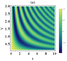
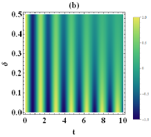
Figure 2: (a)Population difference, $\Delta P$=$P_{1,1}$-$P_{1,2}$ as a function of time $t$, and coupling energy, $V$ at dissipation rates $\gamma_{d1}=\gamma_{d2}$=0.1, for the degenerate case ($\omega_{b2}$=$\omega_{b1}$). The units are chosen such that $\hbar$=1, $\Delta_{1}$=$\Delta_{2}=1$ (i.e $\delta_{1}$=$\delta_{2}$=0.1). Time $t$ is obtained as multiple of $t_{0}$, the inverse of $\Omega_{0}$ (at $\gamma_{d1}=\gamma_{d2}$=0.1) (b) Population difference, $\Delta P$=$P_{1,1}-P_{1,2}$ as a function of time $t$, and deviation factor, $\delta=\delta_{2}$ at tunneling energy $V$=1, $\gamma_{d1}$=0 and $\Delta_{2}$=1.

The decay branching ratio is quantified by the fraction $F_{1}$ (or $F_{2}$) of a $N$-state composite boson that decay via $\gamma_{d1}$ (or $\gamma_{d2}$). $F_{2}$ is evaluated using Parseval’s theorem statt

$$F_{2} = \gamma_{d2}\;\int_{-\infty}^{\infty}\frac{dE}{2\pi}|G_{1,2}(E)|^{2},$$ (28)

$$= \frac{(1+\frac{\gamma_{d2}}{\gamma_{d1}})V^{2}}{{\omega_{0}}^{2}+\gamma_{d}^{2}(1+\frac{4V^{2}}{\gamma_{d2}\gamma_{d1}})}.$$ (29)

The fraction $F_{1}$=$1-F_{2}$. Results displayed on Fig. 3a show the increase (decrease) in the branching fraction $F_{2}$ due to increase (increase) in the bosonic deviation measure $\delta_{2}$ ($\delta_{1}$) for fixed values of the energy difference $\omega_{0}$ and tunneling energy $V$. Fig. 3b shows the notable decrease of the branching fraction $F_{2}$ with increase in the energy difference $\omega_{0}$. Conversely, the branching fraction $F_{1}$ increases with increase in the energy difference $\omega_{0}$, as expected.

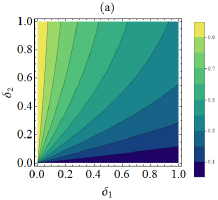
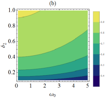
Figure 3: (a) Branching fraction $F_{2}$ of a $N$-state composite boson that decay via $\gamma_{d2}$ as a function of bosonic deviations, $\delta_{1}$ and $\delta_{2}$. Energy difference $\omega_{0}$=$\omega_{b2}$-$\omega_{b1}$=0.5, and tunneling energy $V$=1. (b) Fraction $F_{2}$ as a function of energy difference $\omega_{0}$ and bosonic deviation, $\delta_{2}$. The tunneling energy $V$=5 and $\delta_{1}$=0.1. The units are chosen such that $\hbar$=1, $\Delta_{1}$=$\Delta_{2}=1$ for both figures.

VII Application to pigment protein complexes in light-harvesting systems

It is useful to analyze the results obtained in Section VI in the context of large photosynthetic membranes which constitute many biological pigment-protein complexes (i.e., chromophores) such as FMO (Fenna-Matthews-Olson) complexes in the green sulphur bacteria adolp ; flem . The FMO complex trimer is made up of three symmetry equivalent monomer subunits, with each unit constituting eight bacteriochlorophyll (BChl)a molecules supported by a cage of protein molecules. The FMO complex acts as an efficient channel of excitation transfer in which photons captured in the chlorosome which is the main light harvesting antenna complex, are directed via a series of excitonic exchanges to a reaction center (RC) where energy conversion into a chemical form occurs. Long-lived coherences between electronic states lasting several picoseconds, much shorter than the $1$ ns dissipative lifetimes of excitons flem , have been a topic of intense investigation in recent years silbey ; recom ; thilhs1 ; thilhs2 . Currently it is still not clear as to how biological systems comprising hundreds of photosynthetic complexes and many more correlated excitonic states act in unison to maintain the quantum coherences in the noisy environment, and attain the much envied high efficiencies at psychological temperatures.

In the FMO complex, the chromophore sites numbered $3$ and $4$ are located near the reaction center, and thus are closely linked to the sink region where energy is released, while chromophore sites $1$ and $2$ are strongly coupled, and dissipate energy via site $3$ adolp . The sites $1$, $6$, and $8$ are located at the baseplate which connects to the chlorosomes that receive electronic excitation. Recently, it was shown that the eighth chromophore (at site $8$) is located nearer the chromophore sites of neighbouring monomers compared to sites in its own monomer olb . This indicates a stronger inter-monomer (as compared to intra-monomer) interaction as far as the eighth chromophore is concerned and the excitation at site $8$ is likely to propagate to a inter-site monomer (see Fig. 4a ). It was pointed out olb that the eigth chromophore acts to facilitate excitation transfer between monomers of the FMO trimer even though it is best placed to receive excitation at the earliest time. To this end, the eighth chromophore appears to play a critical role in the topological connectivity of large molecular structures of multichromophoric macromolecule (MCMM) systems. The electro-optical properties of these MCMMs vary from those of single chromophores, depending on the delocalization of excitons within each MCMM.

Here we apply Eq. (26) to a model in which excitons in MCMMs undergo tunneling dynamics over distances that are large compared to the average distance between chromophores within the FMO monomer/trimer configurations barz . A simple setup is shown in Fig. 4b, where $1<N<N_{m}$=24, and which describes the system of composite bosons in one FMO trimer that is considered as the multichromophoric macromolecule. Individual MCMM can be coupled to each other as is shown for two FMO trimers in Fig. 4b. Dissipation may arise from Pauli exchanges between the FMO pigments and the protein bath, and recombination and trapping effects specific to each macromolecular system. The configuration Fig. 4b can be further extended to one in which each MCMM includes several trimers forming aggregates. The net dissipation within each MCMM may vary from other similarly configured MCMM, depending on the connectivity and proximity to the region of light illumination. In a recent work sener , multiple detrapping/retrapping processes as opposed to the slow (200 ps) direct transfer between RCs in the purple bacterium Rhodobacter sphaeroides sener were noted to contribute to the delocalization of excitation among several reaction centres (RCs). In this regard, the tunneling energy $V$ in Eq. (26) may be based on a cumulative process of repeated trapping/detrapping events instead of a single direct transfer mechanism.

Oscillations between MCMMs are expected as shown in Fig. 2a,b, with excitation exchanges that gradually fades with time depending on the initial conditions, dissipation parameters, $\gamma_{d1},\gamma_{d2}$ (specific to the two MCMM sites) and average energy difference ($\approx\omega_{0}$) between the MCMM sites. As noted earlier, coherence times are much shorter than the dissipative lifetimes of excitons flem . Of particular interest is use of the branching ratio in Eq. (29), which identifies effective routes of energy propagation in large topologically connected network structures. A single antenna complex may serve several FMO complexes, and a reaction center may be linked to several FMO trimers. Selective MCMM sites which function as collection centers may experience greater dissipation than other sites and possess higher branching ratios (Fig. 3a,b). Such sites contribute to a structural arrangement that enable photosynthetic organisms to better utilize cellular resources.

Continued coherence in photosynthetic complexes is ensured by a small bosonic deviation measure $\delta$ and large number $N$ of fermion pairs involved during energy exchanges (Fig. 2). This suggest that a molecular environment that is highly correlated, with a large Schmidt number ${\cal K}$ (Eq. (2) is likely to preserve electronic coherences needed for propagation of excitation such that energy is harvested efficiently. The spectral and molecular dynamics of MCMM at various lattice temperatures and excitation densities (light illumination) appear to influence the kinetics of exciton and electron-hole pair recombination and relaxation processes. These can be seen as critical factors that influence the Schmidt number ${\cal K}$ specific to a MCMM. Thus far, we have considered a few factors which underpins the high efficiencies noted in light-harvesting systems, on qualitative terms. A quantitative approach would involve modeling the realistic condition of an entire photosynthetic membrane constituting many FMO complexes, and taking into account the topological connectivity of thousands of bacteriochorophylls. The approach taken in this work is expected to help understand the importance of the coexistence af boson and fermionic phases, Pauli scattering effects and selective dissipation in photosynthetic systems.

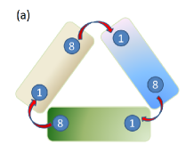
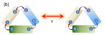
Figure 4: (a) Simplified trimer configuration in which the eighth chromophore is positioned close to the first chromophore of a neighbouring monomer, resulting in a stronger inter-monomer (as compared to intra-monomer) interaction for an excitation at site $8$ olb . (b)A system of two coupled FMO trimer multichromophoric macromolecules that is capable of displaying long-lived coherences for small bosonic deviations of composite excitons at each trimer site.

VIII Conclusion

In conclusion, the quantum dynamics of conversion of composite bosons into fermionic fragment species is demonstrated using an open quantum system approach based on a system-plus-reservoir model. The total Hilbert space which constitutes a composite boson subspace and an orthogonal fragment subspace of fermions pairs is used to examine the effect of system parameters during the tunneling dynamics of coupled composite bosons states. The results highlight the interplay of boson and fermionic phases that is dependent on density (and indirectly the network connectivity) and lattice temperature, and the appearance of exceptional points based on experimentally testable conditions (densities, lattice temperatures). The effect of Pauli exclusion and other dissipative factors on the multichromophoric macromolecules (MCMMs) in photosynthetic light harvesting is examined in the light of quantitative results obtained for coupled composite bosons systems. It is noted that long-lived quantum coherence in photosynthetic complexes is assisted by small bosonic deviation measures (large Schmidt number) and large number of excitons involved during energy exchanges, to give rise to a highly correlated molecular environment. Moreover, specific MCMM sites which function as collection centers may possess higher branching ratios, and contribute to a structural arrangement that enable photosynthetic organisms to better harness solar energy efficiently.

IX Acknowledgments

A. T. gratefully acknowledges the support of the Julian Schwinger Foundation Grant, JSF-12-06-0000, and thanks M. Combescot for useful correspondences on specific properties of composite bosons and related references.

X References

References

- (1) A. Imamoglu, Phys. Rev. B 57 R4195 (1998).
- (2) A. Thilagam, Phys. Rev. B 59, 3027 (1999).
- (3) M. Combescot, O. Betbeder-Matibet, and F. Dubin, Phys. Rev. A 76, 033601 (2007).
- (4) M. Combescot, O. Betbeder-Matibet, and F. Dubin, Phys. Rep. 463, 215 (2008).
- (5) M. Combescot and O. Betbeder-Matibet, Phys. Rev. Lett. 104, 206404 (2010).
- (6) M. Combescot, S.-Y. Shiau, and Y.-C. Chang, Phys. Rev. Lett. 106, 206403 (2011).
- (7) H. Deng, H. Haug, Y. Yamamoto, Review of Modern Physics, 82, 1489 (2010).
- (8) F. P. Laussy, M. M. Glazov, A. Kavokin, D. M. Whittaker, and G. Malpuech, Phys. Rev. B 73, 115343 (2006).
- (9) C. A. Regal, C. Ticknor, J. L. Bohn, and D. S. Jin, Nature 424, 47 (2003).
- (10) K. E. Strecker, G. B. Partridge, and R.G. Hulet, Phys. Rev. Lett. 91, 080406 (2003).
- (11) C. K. Law, Phys. Rev. A 71, 034306 (2005).
- (12) C. Chudzicki, O. Oke, W. K. Wootters, Phys. Rev. Lett. 104, 070402 (2010).
- (13) S. S. Avancini, J. R. Marinelli, and G. Krein, J. Phys. A: Math. Theor. 36, 9045 (2003).
- (14) P. Sancho, J. Phys. A: Math. Theor. 39, 12525 (2006).
- (15) R. Ramanathan, P. Kurzynski, T.K. Chuan, M.F. Santos, and D. Kaszlikowski, Phys. Rev. A 84, 034304 (2011).
- (16) A. Gavrilik and Y. Mishchenko, Phys. Lett. A 376, 1596 (2012).
- (17) M. C. Tichy, F. Mintert, and A. Buchleitner, J. Phys. B: At. Mol. Opt. Phys. 44, 192001 (2011).
- (18) N.F. Mott, Philos. Mag. 6, 287 (1961).
- (19) R. Zimmermann, Many-Particle Theory of Highly Excited Semiconductors, (Leipzig: Teubner), (1988).
- (20) D. Semkat, F. Richter, D. Kremp, G. Manzke, W.-D. Kraeft, and K. Henneberger, Phys. Rev. B 80, 155201 (2009).
- (21) E. K. U. Gross, O Heinonen, E. Runge,Many-particle theory , Imprint Bristol : Hilger, (1991).
- (22) G. Lindblad, Commun. Math. Phys. 48, 119 (1976).
- (23) V. Gorini, A. Kossakowski, and E. Sudarshan, “Completely positive dynamical semigroups of n-level systems,” Journal of Mathematical Physics, vol. 17, no. 5, pp. 821 825, 1976.
- (24) H. J. Carmichael, Phys. Rev. Lett. 70, 2273 (1993).
- (25) J. Dalibard, Y. Castin, and K. Mölmer, Phys. Rev. Lett 68, 580 (1992).
- (26) H. Feshbach, Ann. Phys 5, 357 (1958).
- (27) B. A. Lippmann and J. Schwinger, Phys. Rev. 79, 469 (1950).
- (28) A. Suna, Phys. Rev. 135, A111 (1964).
- (29) H. T. Ng and S. I. Chu, Phys. Rev. A 85, 023636 (2012).
- (30) M. Greiner, O.Mandel, T. Esslinger, T.W. H ansch, and I. Bloch, Nature (London) 415, 39 (2002).
- (31) B. P. Anderson and M. A. Kasevich, Science, 282, 1686 (1998).
- (32) H T Ng and S Bose, J. Phys. A: Math. Theor. 43 072001 (2010).
- (33) A. Micheli, D. Jaksch, J. I. Cirac, and P. Zoller, Phys. Rev. A 67, 013607 (2003).
- (34) J. Adolphs and T. Renger, Biophys. J., 91, 2778 (2006).
- (35) H. Lee, Y-C. Cheng, G.R. Fleming, Science, 316, 1462 (2007).
- (36) J. Wu, F. Liu, Y. Shen, J. Cao and R. J. Silbey, New J. Phys.12,105012 (2010).
- (37) X. Chen and R. J. Silbey, J.Chem.Phys 132, 204503 (2010).
- (38) A. Thilagam, J. Chem. Phys. 136, 065104 (2012).
- (39) M. Combescot, Europhys. Lett. 96, 60002 (2011).
- (40) E. Schmidt, Math. Annalen 63, 433. (1906).
- (41) B. Terhal and P. Horodecki, Phys. Rev. A 61, 040301(2000).
- (42) A. Sanpera,D. Bruß, D., M. Lewenstein, Phys. Rev. A, 63, 050301(2001).
- (43) G. C. Ghirardi, L. Marinatto, Optics and Spectroscopy 99, 386 (2005).
- (44) R. J. Glauber, Phys. Rev. 130, 2529 (1963).
- (45) F. P. Laussy, M. M. Glazov, A. Kavokin, D. M. Whittaker, and G. Malpuech, Phys. Rev. B 73, 115343 (2006).
- (46) M. Combescot, O. Betbeder-Matibet, Phys. Rev. Lett.93, 016403 (2004)
- (47) A. Thilagam, Phys. Rev. B 55, 7804 (1997).
- (48) A. Thilagam and A. R. U. Devi, J. Chem. Phys. 137, 215103 (2012).
- (49) S. Maniscalco and F. Petruccione, Phys. Rev. A 73, 012111 (2006)
- (50) A. Shabani and D.A. Lidar, Phys. Rev. A 71, 020101(R) (2005).
- (51) W. D. Heiss and A L Sannino, J. Phys. A: Math. Gen. 23 1167 (1990).
- (52) C. A. Stafford and B. R. Barrett, Phys. Rev. C 60, 051305 (1999).
- (53) A. Thilagam, J. Chem. Phys. 136, 175104 (2012).
- (54) C. Olbrich, T. L. C. Jansen, J. Liebers, M. Aghtar, J. Strümpfer, K. Schulten, J. Knoester and U. J. Kleinekathöefer, Phys. Chem. B 115, 8609 (2011).
- (55) M. K. Sener, J. D. Olsen, C. N. Hunter, and K. Schulten, Proc. Natl. Acad. Sci. U.S.A. 104, 15723 (2007).
- (56) V. Barzda,G. Garab, V. Gulbinas, L. Valkunas, Biochimica et Biophysica Acta 1273, 231 (1996).