Abstract

The central institute of electronics (ZEA-2) in the Forschungszentrum Jülich (FZJ) has developed the novel readout electronics JUDIDT [1] to cope with high-rate data acquisition of the KWS-1 and KWS-2 detectors in the experimental Hall at the Forschungsreacktor München FRM-II [2] in Garching, München.

This electronics has been then modified and used also for the data-acquisition of a prototype for an ANGER Camera [3] proposed for the planned European Spallation Source. To commission the electronics, software for the data acquisition and the data monitoring has been developed. In this report the software is described.

Forschungszentrum Jülich

Internal Report No. XXX

1 Introduction

This note describes how to install and to use the DAQ program suite developed for the Neutron and Gamma Detector Group (Arbeit Gruppe Neutron und Gamma Detektoren, AGNuGD) at ZEA-2 in FZJ. The documentation also provides a description of how the code is structured with the scope to give to the future developers the possibility to easily implement modifications and further developments.

The program was initially developed for the commissioning of the JUDIDT2 [1] electronics, designed and manufactured at ZEA-2, to be used as a readout system for an ANGER Camera prototype within the XX Collaboration. During the commissioning its functionality was extended to perform spectrum analysis of plastic scintillators by using the ACQIRIS digitizers. The description here given refers to the software version V2.0. Later changes and implementations should not invalidate the main procedures here shown.

2 Installation of the DAQ Software

The suite is distributed as a zip archive DAQ_Vxx.zip (the tag xx referring to the version number, as 0.1, 0.2, and so on). After copying the zip file to the wanted location, the archive can be unzipped (under Linux man can use the command “unzip <zip_file>”) and the directory DAQ_Vxx will be there unpacked. In that root directory the sub-directories of each of the DAQ programs are found, and they contain the source code for their build:

1. LIB_JUDIDT
   ==> library of the JUDIDT electronics;

2. DAQ_LIB
   ==> library of the DAQ;

3. DAQ_SERVER
   ==> the DAQ Server;

4. DAQ_CLIENT
   ==> the DAQ Client in terminal mode and the libSocket;

5. DAQ_CLIENT_GUI
   ==> a graphical interface to communicate with the SERVER;

6. ONLINE_MONITOR
   ==> the graphical monitor to watch the data online (or the data previously taken);

7. RUNLOG
   ==> the GUI to store in an external file information on the runs.

These programs above listed are the main constituents of the DAQ suite, and are described in the sections 4.x.

Additional folders and files are present in the unzipped folder. One group is needed to build the software, and it is foreseen to provide the necessary flexibility to be platform independent. Tools to compile with gcc, nmake, Visual Studio and the QT IDE are given. In principle, the QT environment should provide a cross-platform framework, being its configuration files (.pro files) configured to compile in both Linux and Windows systems. By using QT functions many calls are already cross-platform; for example, from the Client GUI external programs (as the DAQ server or the Online Monitor) can be started. The reference build system is QT, while the other frameworks are periodically but not regularly updated, and their maintenence is not regularly ensured.

The compilation folders and scripts are the following:

1. Makefile.gcc
   ==> the script to compile the packages with gcc

2. Makefile.nmake
   ==> the script to compile the packages with nmake

3. QT_CREATOR
   ==> the folder with the configuration files (*.pro) to compile within the QT IDE

4. VS2008
   ==> the folder with the configuration files (*.vcproj) to compile within Visual Studio

5. bin
   ==> where the executables are locally stored

6. include
   ==> include files common to more packages

7. lib
   ==> libraries locally stored

8. CONFIGURE
   ==> Configuration files are here stored:

   • configure.sh
     ==> to perform the initial configuration in Linux

   • configure.bat
     ==> to perform the initial configuration in Windows  .

As first step the user has to run the configure.sh(.bat) script in order to create some relevant folders. Under Linux the installation of the libraries should require root privileges. During the configuration the following three directories are created, according to which operating system is running (Linux, XP, or the CYGWIN environment for XP):

1. Where the binary files of the accumulated data are stored

   • Linux:
     ==> /scratch/DAQ_REPOSITORY

   • XP:
     ==> c:\DAQ_REPOSITORY

   • XP/CYGWIN:
     ==> /scratch/DAQ_REPOSITORY

2. Where the executables will actually run, and where the program configuration files are located

   • Linux:
     ==> /scratch/DAQ_WORKING_DIR

   • XP:
     ==> c:\DAQ_WORKING_DIR

   • XP/CYGWIN:
     ==> /scratch/DAQ_WORKING_DIR

3. Where the executables are globally located

   • Linux:
     ==> /home/<user_home_directory>/bin

   • XP:
     ==> c:\bin

   • XP/CYGWIN:
     ==> /home/<user_home_directory>/bin  .

Note that to compile the drivers for the JUDIDT2 readout system the driver, library and include files for the Plx tools should be present in the system. The Plx tools are needed to control the FPGA in the SYS interface and in the JUDIDT2 module. See the JDAQ.pro file in the QT_CREATOR/LIB_JUDIDT for clarifications. The same applies for the ACQIRIS system. In addition, also the libraries and the includes of ROOT [5] developed at CERN are needed, because the GUI packages are built against those libraries, exploiting their long and mature development to fulfill the requirements of the analysis in several fields of physics. Please note that when using external libraries as the ROOT ones, the same compiler should be used to correct identify the symbols of the used objects saved in the library.

When no error appears during the compilation, then all the packages should have been located in the installation directory, which was setup during the initial configuration procedure.

Additional folders and files are present:

1. DOCUMENTS
   ==> contains this and additional documentation;

2. README
   ==> A short description about how to compile all packages

3 Overview of the DAQ Programs

This DAQ programs are structured in a client-server framework, as shown in Fig. 1. The server (DAQServer) runs listening to clients (DAQClient), which send it commands via a socket [4]. It is eventually the user-level interface to a shared library which interacts with the low-level driver of the selected readout system.

Figure 1: Structure of the client-server architecture of the DAQ.

As soon as the DAQ starts, the data are stored in binary format into a file saved in the DAQ_REPOSITORY directory. The data can be online or offline inspected by the online monitoring GUI (OnlineMonitor), based on the ROOT libraries.

In principle all the DAQ operations can be done in terminal mode, in cases when the amount of computer resources (CPU and memory) could be an issue. A friendly GUI (DAQClientGUI), based on ROOT, has been also developed to control, directly from its menu, the data acquisition and the online monitoring.

The modular structure of this DAQ suite provides many advantages with respect to having a single block of software. It allows in fact the implementation of changes to single parts, without altering the remaining components. As an example, the OnlineMonitor could be implemented using graphical libraries different from ROOT, e.g. using the LabView interface, or additional features of the program can be written without the need of modifying the DAQ server and clients.

On the other side, when a fast monitoring of the data (e.g. at acquisition rates as fast as the Megahertz) is needed then possibly this solution appears to be not the best, being the data acquisition delayed by the continuous i/o to the database (for example a file).

4 DAQ Server

The server (DAQServer) is a terminal mode program, which can be started either directly from a terminal (Fig. 2), or using the main user GUI. Note that this last option also opens a terminal.

Figure 2: The server is here started directly from a terminal.

As soon as the server is started, a LOG file is opened in the DAQ_WORKING_DIR, and every activity executed is recorded there. The LOG file can be online accessed under Linux via ’tail -f DAQ_WORKING_DIR/DAQServer.log’.

The server then opens a socket at the port 5540 (this number is for the moment hardcoded), and starts to listen at commands sent by any number of independent clients.

When a command is received, either to configure the hardware or the data acquisition, the server calls the relevant function in the DAQ library. Here, according to the used readout system the corresponding proper function is used; at the server side every command disregards the underlining hardware; it is the DAQ library which takes care to use the proper driver with respect to the readout system.

5 DAQ Client

The client (DAQClient) is a simple program which takes as command line argument an option and, when needed, its value. Via a socket the command is sent to the server which, after processing it, sends back the answer to the received command, which could be also a value of the hardware configuration. This communication is done using the DAQSocket library.

In case no option is sent an error is dumped to the terminal. To know which commands are available the option ’-help’ should be used (see the bottom right terminal in the screenshot shown in Fig. 3), and a list of options will be dumped to the server LOG file (leftmost displayed terminal in the picture).

Figure 3: Example of sending a command to the server. The user via a client asks the server for the list of the available options, which is dumped into the LOG file by the server.

After receiving the answer from the server the client always exits. Commands can be sent to the server by, in principle, ’infinite’ clients, each one running in an independent terminal. This is possible because what is important here to communicate with the server, is the existence of a socket at a specific port.

To start (stop) the data acquisition, the user should simply sending the command ’-start’ (-stop) to the serve. The default run number is taken to be the largest already stored run number, increased by one unit.

6 The DAQ Socket Library

As previously mentioned, the communication between server and clients is based on a library (libSocket.so/libSocket.dll) which uses a socket for exchanging information between them. The working principle of a socket is based on the transmission of character strings via virtual channels (i/o ports for the operating system). A shared library function with three arguments is used for this purpose. The library arguments are pointers to strings.

A command is transmitted to the server giving the socket library the pointer to the command string as its first argument. The second and third arguments are the pointers to additional strings. The library acknowledges to have received a certain command using the string which is pointed by the second argument of the library. It sends then the command string to the server via the socket, and it remains active waiting for the answer from the server via the opened socket. The received string is copied to the allocated memory pointed by the third argument of the library. The client can now retrieve the server answer accessing this last address. The memory needed for these strings is allocated by the client before issuing a command.

7 The Main User Frontend: DAQClientGui

A graphical interface (based on the ROOT libraries) was developed to help the user to access all the main components of the DAQ the server. As shown in the screenshot of Fig 4, directly from the GUI the DAQ can be started and closed, the readout system can be chosen (at the moment only the JUDIDT and the ACQIRIS systems are implemented), and the OnlineMonitor program can be launched from there.

Figure 4: Directly from the GUI the DAQ can be started and closed, the readout system can be chosen and the OnlineMonitor program can be launched from there.

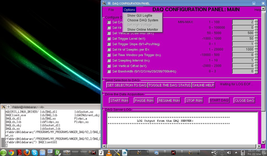
Once a readout system is set (via the option ’Choose DAQ System’ in the menu) then the DAQ setting can be configured by activating the relevant buttons and choosing the corresponding values in the main panel. The selection done can be set to the hardware clicking the ’SET SELECTION TO DAQ’ button. The status of the DAQ can be always be accessed using the button ’TOGGLE THE DAQ STATUS’ or scrolling the output in the server LOG file displayed in the ’DAQ Server LOG’ panel. Note that the DAQ configuration can be performed only when data acquisition is not running. This is because all the data in a run should be accumulated with the same configuration, which is saved in the header of the run file.

The LOG activity of this GUI can be accessed in a separate canvas via the menu option ’Show GUI Logfile’. The Help option gives the user the possibility to open this documentation in the Acrobat Reader, and the History option displays the progress done during the several versions of the program.

8 The DAQ Library

The DAQ library is possibly the core of this data acquisition software. It is a collection of functions to control the hardware, and according to the selected readout electronics its relevant low-level driver function is called.

When the data acquisition is started, and the data are indeed accumulated, the value for each event in each channel of the hardware is stored in a global structure, whose memory location is returned back to the server at every readout. This will then save the data to an external binary file, clearing the memory allocated by the library, and starting a new hardware readout. The default configuration keeps on accumulating the data also when a run is terminated, increasing automatically the run number of one unit.

Differently from the ACQIRIS system, which allows to store entire waveforms, the JUDIDT electronics provides already the peaking amplitude (calculated by the internal FPGA). The same data structure is maintained by saving the JUDIDT data as single-point waveforms.

In principle, following what done using two systems, the library can be expanded to accommodate additional readout system, keeping the high-level software (Server, Client and OnlineMonitor) almost unaffected by the performed changes. The activity done by the library functions is documented in the server LOG, whose memory address is given to the library functions by the server.

9 The Online Monitor GUI

The friendly graphical user interface OnlineMonitor, based on ROOT, has been developed to control online the quality of the data provided by the data acquisition system, Fig. 5.

Figure 5: The accumulated data can be monitored online and offline directly from a GUI interface. In this example the coincidence of signals from four photomultipliers, originating from a neutron transit in a gas-filled Anger Camera is shown. The photomultipliers are here not yet gain-matched.

With the option ’Live’ active the program monitors the data of the ongoing run (after retrieving the current run number from the server). Previously accumulated data can be analyzed by providing the corresponding run number. An error will be prompted whenever the data file will not be found. In the ’Live’ mode new runs are automatically monitored without any action from the user.

At startup the program reads the steering file ONLINE_MONITOR.conf to give some global variables a value different from the default hard-coded one. The format is the following: <var>%<Value>. At the moment only the choice of the data repository directory is implemented, although in principle additional variables could be there implemented.

The header of the run is shown in the ’Run Configuration’ Tab, as soon as the run is processed, displaying the following slowcontrol parameters:
Run Number Readout System, Start Time of the run Number of readout channels, Number of sampling for waveform Sampling time unit, Delay time Max amplitude accessed ADC resolution Pedestal offset Trigger level (during the DAQ) Trigger slope Line impedance

Additional tabs show, for each input line, the integrated signal charge, the calculated pedestal and noise and the corresponding averaged value vs time average (as well as the rates and the temperature vs time; the temperature is at the moment not readout, and therefore not displayed yet).

During the monitoring the user can choose, as a first rough analysis of the data, to provide a common threshold to all the input channels, either positive or negative.

For documentation purposes, via the ’File’ menu entry, a screenshot of the entire program window, or the histograms in the displayed canvas can be saved. The format of the generated plot is forseen to be chosen in the ’Options’ menu entry (not yet implemented). At the moment the default format is the postscript.

The tab ’Integrated Charge’ shows the calculated total charge integrated by the software in case of the AQUIRIS readout which saves entire waveforms. In case of the JUDIDT system the integration is performed inside the electronic (in this case one measurement point is given every single event readout).

With the ACQIRIS system at the moment the pedestal is calculated also in presence of a neutron signal considering the entire waveform; here the value with the maximum number of counts is considered as pedestal mean. Around this value a small range of signal value is used to generated a distribution whose RMS is considered as system noise during this event. In order to have this technique reliable some data before the risetime of the signal should be accumulated.

In case of the JUDIDT system, a ’Calibration’ flag should be given (via the menu in the DAQClientGUI). Then the data are accumulated via a software trigger and could in principle be considered, e.g. being out of the beam, as system pedestal events. This distribution, expected to be Gaussian, is shown in the ’Pedestals’ Tab.

The mean and RMS for the data collected every minute are used for the calculation of the time dependence of the pedestal and noise in each input line, and are presented in the ’Means vs Time’ Tab. Also, the RMS calculated as above mentioned is used to fill the Noise histogram presented for every readout channel in the ’Noise’ Tab.

At the moment the Tabs ’Integrated Charge’, ’Pedestal’ and ’Noise’ allows to show four channels within the available number of channels in the analyzed run. The possibility to choose the rate for the histogram refresh (which can be time consuming) in those three Tabs and also in the ’Space Points’ Tab is given by th an entry widget: at high DAQ rates a large value is suggested to keep the monitoring updated with the data acquisition. On the other side, in case of weak sources a large refresh value could keep the user waiting too long for a refresh. Please note that a refresh can be always forced by clicking on the ’Update Histo Now’ button in the bottom Status Bar of the GUI. In case of the ACQIRIS system the refresh rate does not affect the waveform display, which is always performed every sequential waveform. In the Status section of the GUI is also present the option ’Reset Histo Content’; in this case the data sofar accumulated in all histograms will be deleted, except for the graphs shown in the ’Means vs Time’ Tab.

An additional canvas can be shown to present the LOG entries generated by the program. To show or hide it the menu option ’Show Logfile’ can be used.

In order to correctly process the data content in the binary file the updated version of the include file DataStructure.h should be used at the compilation time. This issue originates from unwanted but necessary modifications in the run header motivated by the data analysis needs. The old runs have been modified offline considering the latest implementations of the data stream structure.

10 The Data Format

The data are saved in a compressed binary format following the scheme shown in Fig. 6.

Figure 6: Diagram describing the structure of the streamed data saved in the binary file.

The first information which should be saved is the run configuration introduced by the TAG #RUN_CONFIG, and can be interpreted via the C-structure RUN_CONF:

typedef struct {

unsigned long int	RUN_NUMBER;	// Run Number
unsigned long int	RUNSTART_TIMESTAMP;	// Start of the Run
char	READOUT_SYSTEM[8];	// Which Readout System
int	NR_OF_CHANS;	// Nr of Channels
int	NR_OF_SAMPLES;	// Samples in each Event
int	TRIGGER_SLOPE;	// Trigger Slope
int	COUPLING_FLAG;	// Impedance FLAG
double	DELAY_TIME;	// DAQ Window pre-trigger (secs)
double	SAMPLING_INTERVAL;	// Sampling Unit (secs)
double	TRIGGER_LEVEL_LOW;	// Trigger Level
double	Offset;	// Volt Offset
double	FullScale;	// Volt Scale

} RUN_CONF;

A C-call like

"fread( &RUN_CONF, sizeof( RUN_CONF ), 1, POINTER_TO_FILE);"

should allow to fill all the variables declared in the RUN_CONF structure. It is clear that not all variables will obtain a non null value, according to the readout system (e.g. the JUDIDT system in this DAQ system does not save the waveform but only the peaking amplitude, therefore in this case the number of samples per event is one). At this stage all variable objects dynamically allocated which depend on the number of readout channels (e.g. signal, pedestal and noise histograms) are deleted and reallocated according to the new size provided. This operation is performed only once at the beginning of the run.

Soon after the run header should appear the header of the first data readout, and the call

"fread( &DataFlag, sizeof( DataFlag ), 1, POINTER_TO_FILE );"

will fill the C-structure for the data header:

typedef struct {

int	DAQ_TRIGGER;	// Type of data (Normal/Calib)
int	NR_OF_READOUT;	// Readout Counter
unsigned long int	TIMESTAMP;	// Start of the Readout
int	NR_OF_EVENTS;	// Events in each channel
long int	SIZE_OF_STREAM;	// Size of Data Stream

} DATA_FLAG;

After retrieving how many events per channel are stored in a particular readout, the analyzer can read the amplitude value of each event following this "for loop" sequence:

for_loop_over_channels {

for_loop_over_events_in_channel {

for_loop_over_sampling_in_event { // only one with JUDIDT

….

} // Loop over samplings in one event

}       // Loop over events in one channel
}           // Loop over channels

Knowing how to easily read the data from the binary files the analyzer can, in principle, perform also a more detailed analysis on the data with his own code; it is enough to have a single include file.

11 The Run LOG

A small GUI has been developed in Tcl/Tk (due to the flexibility and simplicity of this interpreted language) to store during the data acquisition some information relevant to the ongoing run. A screenshot of the program is presented in Fig. 7.

Figure 7: Screenshot of the GUI DAQ_RunLog.tcl.

At the end of each run the user can set some relevant parameters for the accumulated data, which are then stored in the ascii file RunList.dat when typing "Save run to RunList". Then a new empty form will be presented to the user with the run number increased of one unity.

In case an error is made, there is a menu option to retrieve the previously saved settings for that specific run, and to change them. In the menu there is also the possibility to delete the information of the last saved run, that is of the last record in the ascii file.

Each record of the file refers to a specific run, and contains the values of all the relevant variables designed for a specific project (in this case, the commissioning of the JUDIDT electronics). It is clear that, while the needs of a project might change, different variables could be implemented.

According to the selected run type, Normal (Beam), Calib or Other, a color code marks the cell of the run number. Normal data taking is marked with green; otherwise the yellow code is used. In case a test is made, or the accumulated data are for whatever reason bad and useless, the source of bad quality should be checked in the section "Select source of bad DQ". The run will then be marked with red color.

Some parameters can be set only if they are relevant to the specific type of ongoing run. As an example, if normal data taking is proceeding the calibration section remains inactive, and will be saved in the ascii file as NULL.

The most striking advantage to use such a program is the possibility to easily and fast select subsets of data to analyze without going through all the binary data files.

Although, in the opinion of the author, this interpreted language is really optimal for this type of applications (easy and fast to implement), nevertheless the possibility to convert the program in C/ROOT is considered in future versions. This choice is driven by the advantage to use only one language in the maintenance of the entire package suite.

12 The JUDIDT Library

This library was developed in the ZEL-2 institute, and embedded and tuned in a DAQ code for an Online Monitor based on LabView, thus in a monolithic software needed for a specific project.

In principle, being developed by third parties it should not be mentioned here; nevertheless, for its use in this separate DAQ project some modifications were needed, to keep only the driver for the input/output with the electronics, and to decouple it from the LabView components for the monitoring.

Additional modifications were needed to make the functions of this driver as much as possible consistent with the driver for the ACQIRIS readout, also implemented in this DAQ.

The modified code can be compiled in the DAQ_CLIENT folder in combination with the DAQClient with the compilers gcc or nmake, or even better using the QT development environment in QT_CREATOR/LIB_JUDIDT.

13 Conclusions

We have presented in this note a new software for the data acquisition based on the Server-Client architecture, and based on the socket concept for send and receive commands. All the components of the package were described in separate sections.

It is clear that the code is at the moment not really a general purpose code, being in many parts tuned to the forseen project to investigate the JUDIDT electronics. Nevertheless the code has been designed to be made of separate independent components, and make strong use of pointers (thus of dynamically allocated memory arrays with variable size). This aspect should allow an easier implementation of additional features, if needed in the future.

The publication of the results of the analysis performed on the JUDIDT readout system, also in combination with the Anger Camera prototype is on going [6].

Acknowledgments

The author gratefully acknowledges U. Clemens, R. Engels, and G. Kemmerling for their valuable technical contribution and suggestions to the work here presented.