Accelerating Solitons in Gas-Filled Hollow-Core Photonic Crystal Fibers

Abstract

We found the self-similar solitary solutions of a recently proposed model for propagation of pulses in gas filled hollow-core photonic crystal fibers that includes a plasma induced nonlinearity. As anticipated for a simpler model and using a perturbation analysis, there are indeed stationary solitary waves that accelerate and self-shift to higher frequencies. However, if the plasma nonlinearity strength is large or the pulse amplitudes are small, the solutions have distinguished long tails and decay as they propagate.

I Introduction

Hollow-core photonic crystal fibers (HC-PCFs) can exhibit very interesting properties, such as relatively low loss, low group velocity dispersion and high confinement of light in the core Russell (2003, 2006), while also allowing new nonlinear phenomena associated with the interaction of light and matter filling these fibers. Lately, these HC-PCFs have been filled with gases for purposes of enhancing Raman scattering if a Raman-active gas is used Benabid et al. (2002), or further controlling the total dispersion of the fiber by varying the gas pressure Nold et al. (2010). Furthermore, it has also been shown that few $\mu$J or even picoJ H lzer et al. (2011); Husko et al. (2013) energy optical pulses are sufficient to ionize the gas and produce a plasma, leading to new nonlinear effects such as the blueshifting of the central wavelength of the pulses Fedotov et al. (2007); H lzer et al. (2011). Despite the fact that the soliton shift to higher frequencies has also been reported in other contexts, such as in a line-defect waveguide Colman et al. (2012) and in tapered solid-core photonic crystal fibers Stark et al. (2011), the existence of a blueshift in a Raman-active gas opens new exciting opportunities of controlling the soliton dynamics by two competing processes, one leading to a redshift, usually known as soliton self-frequency shift (SSFS) caused by intrapulse Raman scattering (IRS) Gordon (1986), and the other to a blueshift.

Traditionally, the interaction between light and matter has been studied using computationally demanding methods based on models for the full electric field of the pulse Geissler et al. (1999) but, recently, Saleh et al. presented a model that describes pulse propagation in hollow-core photonic crystal fibers filled with a gas as a pair of coupled equations for the electric field envelope and ionization fraction Saleh et al. (2011). This model, which neglects losses and results from a linearization of the tunneling model for pulse intensities close to the threshold intensity, has proved to be amenable to the application of both numerical and analytical techniques. In effect, by using a perturbation approach the occurrence of the blueshift effect has already been adequately predicted Saleh et al. (2011).

In this work, we present a thorough study of accelerating solitons in gas-filled HC-PCF, extending the results in Saleh et al. (2011). We start with the model proposed by Saleh et al. Saleh et al. (2011), use an accelerating self-similarity variable to obtain an ordinary differential equation (ODE) to which we apply a perturbation approach and solve using a shooting procedure. In this analysis, we have considered the exact solution for the ionization term and our results apply to both zero and nonzero threshold intensities. The dependence on the model parameters, namely, the plasma and Raman strengths, the intensity threshold and the pulse peak value are studied in detail.

II Self-similarity variable and perturbation approach

As mentioned in the introduction, here we will follow Saleh et al. Saleh et al. (2011) and start with the following coupled equations

$$i\frac{\partial\psi}{\partial z}-\frac{\beta_{2}}{2}\frac{\partial^{2}\psi}{\partial t^{2}}+\gamma|\psi|^{2}\psi-\gamma t_{R}(|\psi|^{2})_{t}\psi-\frac{\omega_{p}^{2}}{2k_{0}c^{2}}\psi=0$$ (1)

$$\frac{\partial n_{e}}{\partial t}=(\tilde{\sigma}/A_{\text{eff}})(n_{T}-n_{e})\Delta|\psi|^{2}\Theta(\Delta|\psi|^{2})$$ (2)

where $\psi(z,t)$ is the optical field envelope in units of square root of power, $z$ is the distance along the fiber, $t$ is the time in a reference frame moving with the group velocity at the central frequency $\omega_{0}$, $\beta_{2}$ is the group velocity dispersion parameter, $\gamma$ is the nonlinear parameter, $t_{R}$ is the Raman parameter, $c$ is the vacuum speed of light, $k_{0}=\omega_{0}/c$, $\omega_{p}=[e^{2}n_{e}/(\epsilon_{0}m_{e})]^{1/2}$ is the plasma frequency associated with an electron density $n_{e}(t)$, $e$ and $m_{e}$ are the electron charge and mass, respectively, $\epsilon_{0}$ is the vacuum permitivity and $A_{\text{eff}}$ is the effective mode area. The plasma-induced nonlinearity only occurs for intensities above the threshold intensity $I_{\text{th}}=|\psi|^{2}_{\text{th}}/A_{\text{eff}}$, so that $\Delta|\psi|^{2}=|\psi|^{2}-|\psi|^{2}_{\text{th}}$ and $\Theta$ is the Heaviside step function. $n_{T}$ is the total number density of ionizable atoms, associated with the maximum plasma frequency $\omega_{T}=(e^{2}n_{T}/(\epsilon_{0}m_{e})]^{1/2}$ and $\tilde{\sigma}$ is the photoionization cross-section. This model assumes that the recombination time is longer than the pulse and neglects the ionization induced loss that is small especially for pulses whose maximum is barely above the threshold. The equation (2) may be solved exactly and after an adimensionalization we obtain

$$i\frac{\partial q}{\partial\xi}+\frac{1}{2}\frac{\partial^{2}q}{\partial\tau^{2}}+|q|^{2}q-\tau_{R}(|q|^{2})_{\tau}q-\phi_{T}q\left(1-\text{e}^{-\sigma\int_{-\infty}^{\tau}\Delta|q|^{2}\Theta(\Delta|q|^{2})d\tau^{\prime}}\right)=0$$ (3)

where $q=(\gamma z_{0})^{1/2}\psi$, $\xi=z/z_{0}$, $\tau=t/t_{0}$, $\tau_{R}=t_{R}/t_{0}$, $\phi_{T}=\tfrac{1}{2}k_{0}z_{0}(\omega_{T}/\omega_{0})^{2}$, $\sigma=\tilde{\sigma}t_{0}/(A_{\text{eff}}\gamma z_{0})$, where $z_{0}=t_{0}^{2}/|\beta_{2}|$ is the called the dispersion length and $t_{0}$ is an arbitrary time chosen similar to the pulse duration. Motivated by the observation of blueshifting of the pulses and previous perturbation approaches, we used an accelerating variable $T=\tau+\frac{a}{4}\xi^{2}+b\xi$ and solutions of the form $q(\xi,\tau)=F(T)\exp(i\theta(\xi,T))$, with $F$ and $\theta$ real, and obtained an ODE for $F$

$$F^{\prime\prime}+aTF-DF+2F^{3}-4\tau_{R}F^{2}F^{\prime}-2\phi_{T}F\left(1-\text{e}^{-\sigma\int_{-\infty}^{T}\Delta F^{2}\Theta(\Delta F^{2})dT^{\prime}}\right)=0,$$

and the following expression for the phase

$$\theta(\xi,T)=-\left(\frac{a}{2}\xi+b\right)T+\frac{1}{2}(D+b^{2})\xi+\frac{1}{4}ba\xi^{2}+\frac{1}{24}a^{2}\xi^{3}+E$$ (4)

where $D$ and $E$ are arbitrary constants. In order to reduce the number of parameters, we introduced the following change of variables $P(\zeta)=\sigma F(T)$ and $T=\sigma\zeta$, with which the ODE for $P(\zeta)$ reads

$$P^{\prime\prime}+\alpha\zeta P-CP+2{P^{3}}-{\gamma_{R}}{P^{2}}P^{\prime}-{\gamma_{P}}P\left({1-{{\text{e}}^{-\int_{-\infty}^{\zeta}{\Delta{P^{2}}\Theta(\Delta{P^{2}})d\zeta^{\prime}}}}}\right)=0$$ (5)

with $\alpha=a{\sigma^{3}}$, ${\gamma_{R}}=4\tau_{R}/\sigma$ and ${\gamma_{P}}=2{\phi_{T}}{\sigma^{2}}$. If we further define

$${\gamma_{P}}=\chi,\quad{\gamma_{R}}=R\chi$$

where $R=\gamma_{R}/\gamma_{P}$, it will permit the application of a perturbation approach simultaneously to the two terms, namely, Raman and plasma, as long as $\chi$ is small.

Hence, we have used a perturbation approach around the ODE associated with the nonlinear Schrödinger equation (NLSE) whose results are valuable by themselves if the additional terms are small, but that also serve as first estimates for our shooting method. Hence, we consider expansions for $P$ and $\alpha$ in powers of $\chi$ such that

$$P=G(\zeta-\zeta_{0})+\chi P_{1}(\zeta)+\cdots,$$

where $G(\zeta-\zeta_{0})=\sqrt{C}\text{sech}(\sqrt{C}(\zeta-\zeta_{0}))$ and

$$\alpha=\chi\alpha_{1}+\cdots$$

and introduce them in (5). To first order, we obtain

$$P_{1}^{\prime\prime}-CP_{1}+6G^{2}P_{1}=-\alpha_{1}\zeta G+RG^{2}G^{\prime}\\ -G\left(1-\text{e}^{-\int_{-\infty}^{\zeta}(G^{2}-P_{\text{th}}^{2})\Theta(G^{2}-P_{\text{th}}^{2})d\zeta^{\prime}}\right)$$

The left member of the last equation is obeyed by $G^{\prime}$, so that, the solvability condition is

$$\alpha_{1}\int_{-\infty}^{\infty}\zeta GG^{\prime}dt=R\int_{-\infty}^{\infty}G^{2}(G^{\prime})^{2}d\zeta\\ +\int_{-\infty}^{\infty}GG^{\prime}\left(1-\text{e}^{-\int_{-\infty}^{\zeta}(G^{2}-P_{th}^{2})\Theta(G^{2}-P_{\text{th}}^{2})d\zeta^{\prime}}d\zeta\right),$$

which gives

$$\alpha_{1}=-\frac{4}{15}RC^{2}+\frac{\text{e}^{-\sqrt{C-P_{\text{th}}^{2}}+P_{\text{th}}^{2}\zeta_{1}}}{\sqrt{C}}\int_{-\zeta_{1}}^{\zeta_{1}}GG^{\prime}\text{e}^{-\sqrt{C}\text{tanh}(\sqrt{C}\zeta^{\prime})+P_{\text{th}}^{2}\zeta^{\prime}}d\zeta^{\prime}\\ +\frac{P_{\text{th}}^{2}}{2\sqrt{C}}\left(1-\text{e}^{-2\sqrt{C-P_{\text{th}}^{2}}+2P_{\text{th}}^{2}\zeta_{1}}\right)$$ (6)

where $\zeta^{\prime}=\zeta-\zeta_{0}$ and $\zeta_{1}$ is the instant at which $G(\pm\zeta_{1})=P_{\text{th}}$. The integral in the last expression may be written in closed form as a series but here we solve it numerically. Nevertheless, for $P_{\text{th}}=0$, the integral is easily solved analytically such that $\alpha_{1}$ simplifies to

$$\alpha_{1}=-\frac{4}{15}RC^{2}-(C^{-1/2}-1)+(C^{-1/2}+1)\text{e}^{-2\sqrt{C}}.$$ (7)

In the limit of small $C$, this equation reduces to $\alpha_{1}=-\frac{4}{15}RC^{2}+\frac{2}{3}C$. Moreover, a graphical inspection of expression (7) shows that it is always below the curve $\frac{2}{3}C$ and in fact it tends to 1 as $C$ increases. On the other hand, whenever the peak intensity is close to the intensity threshold, i.e., $\sqrt{C}\sim P_{\text{th}}$, we may expand the exponentials in equation (6) up to first order and obtain

$$\alpha_{1}=-\frac{4}{15}RC^{2}+\frac{2}{3\sqrt{C}}(C-P_{\text{th}}^{2})^{3/2}.$$ (8)

Note that both this expression and the approximate expression for the acceleration for small $C$ and $P_{\text{th}}=0$ exhibit $C^{2}$ and $C$ dependencies which are associated, respectively, to Raman and plasma effects. Such dependencies imply that the plasma effect is expected to dominate for small peak amplitude pulses, with the acceleration taking positive values which are proportional to the square of the peak amplitude. Conversely, as the peak amplitude increases, the soliton trajectory should be mainly controlled by Raman effect, which leads to a negative acceleration that is dependent on the forth power of the peak amplitude.

III Pulse profiles and accelerations

We then used a shooting method to obtain the pulse solutions of equation (5) and respective accelerations. For this purpose, we first analyse the asymptotical form of this equation for pulse solutions that vanish at the limits $\zeta\rightarrow\pm\infty$ which is given by

$$P^{\prime\prime}+(\alpha\zeta-C-\chi\Lambda_{\infty})P=0,$$

where

$$\Lambda_{\infty}=\left\{\begin{array}[]{lcr}0&\text{if}&\zeta\rightarrow-\infty\\ 1-\text{e}^{-\int_{-\infty}^{\infty}\Delta{P^{2}}\Theta(\Delta{P^{2}})d\zeta^{\prime}}&\text{if}&\zeta\rightarrow\infty\end{array}\right.$$

that, using $z=-\alpha^{1/3}\zeta+\alpha^{-2/3}(C+\chi\Lambda_{\infty})$, may be transformed to an Airy equation:

$$P^{\prime\prime}-zP=0.$$

This result anticipates that the pulse solutions with $\alpha>0$ have tails that are exponentially decreasing as $\zeta\rightarrow-\infty$ as the Airy solution Ai$(z)$ for $z\rightarrow\infty$ and may have tails that are also exponentially decreasing as $\zeta$ increases as the solution Bi$(z)$ for $z\rightarrow 0^{+}$ but that eventually exhibit Airy oscillations (even if very, very small). For $\alpha<0$, the contrary is true.

Considering those asymptotic behavior, we designed our shooting procedure as follows. First, we have fixed the acceleration $\alpha$ and, starting from the left tail, we integrated forward using initial conditions that conform with the corresponding Ai$(z)$. The actual location of the pulse in the $\zeta$ axis may be estimated using the perturbation approach described in the previous section but, since it is not very far from $\zeta=0$, the first estimate for the left tail location $\zeta_{\text{minus}}$ may be obtained as if $P(\zeta)\sim G(\zeta)$. Then, the shooting procedure checks if $P$ and $P^{\prime}$ are already very small at some point in the right tail, and improve the starting $\zeta$ in order to obtain the actual pulse profile for the chosen acceleration. Therefore, this procedure allow us to establish the relationship between the acceleration and the pulse characteristics, namely, its peak amplitude.

Our results show that, as long as $\chi$ is small, the dependence of the acceleration on the peak amplitude is in fact very similar to the one obtained by perturbation, that is, by using expressions (6) or (7) with $\sqrt{C}$ replaced by $P_{\text{peak}}$. Let us first discuss the results for $P_{\text{th}}=0$. Figure 1 shows the acceleration as function of peak amplitude of $P(\zeta)$ for three different strengths of the plasma term and without the Raman term. As shown, the acceleration increases with the amplitude of the peak and a good agreement exists between the shooting results and the perturbation expression (7). Nevertheless, for $\chi=0.3$ there is an observable difference between the two results that can be attributed to the deviation of the pulse profile from the sech shape considered in equation (7). The absence of results for low $P_{\text{peak}}$ in the curves for $\chi=0.2$ and $\chi=0.3$ is due to the inability of our shooting to find a solution with a small right tail. In fact, the pulse profiles with small amplitude are located close to the zero of the Airy $z$ axis, effect that is more pronounced as $\chi$ grows. This means that, in those situations, the solution is no longer similar to a sech profile but it has long, and eventually oscillatory, tails. Figure 2 presents two sets of solutions for $P_{\text{peak}}\sim 0.3$ and $P_{\text{peak}}\sim 0.8$. The first set shows considerable differences at the right tail, with the pulse for $\chi=0.2$ having a longer tail. In the second set, the shape differences are not so evident since for this peak amplitude, both solutions are already similar to each other and with the sech shape.

Figure 1: Dependence of acceleration parameter $\alpha$ on the pulse peak amplitude for $P_{\text{th}}=0$ and for three different $\chi$ values. Points are shooting results and lines are for the perturbation expression.

Figure 2: Pulse profiles with peak amplitude close to (a) 0.3 and (b) 0.8 for two different $\chi$ values.

Concerning the numerical results for $P_{\text{th}}\neq 0$, the accelerations are again in good agreement with the perturbation expression if $\chi$ is small. As figure 3 shows, when compared with the results for $P_{\text{th}}=0$, the accelerations are lower for small peak amplitudes and larger otherwise. Furthermore, the acceleration decreases with increasing $P_{\text{th}}$ for smaller peak amplitudes and the inverse is true for larger peak amplitudes. Also represented in this figure is the acceleration resulting from the approximate expression (8) with $\sqrt{C}$ replaced by $P_{\text{peak}}$, which, as anticipated, is close to the shooting results when $P_{\text{peak}}\sim P_{\text{th}}$. The pulse shape differs from the sech also for some peak amplitudes close to $P_{\text{th}}$ but this effect is smaller as $P_{\text{th}}$ increases. Note that as $P_{\text{th}}$ increases, the possible peak amplitudes that make the plasma term nonzero are also increasing, since the latter should be larger than the first. Figure 4 compares pulse profiles for $P_{\text{th}}=0$ and 0.2.

Figure 3: Dependence of acceleration parameter $\alpha$ on the pulse peak amplitude for different $P_{\text{th}}$ values and fixed $\chi=0.1$. Points are shooting results and lines are for the perturbation expression (6). The inset shows the shooting accelerations for $P_{\text{th}}=0.2$ compared with $\alpha$ computed using (8) with $\sqrt{C}$ replaced by $P_{\text{peak}}$.

Figure 4: Pulse profiles with peak amplitude close to (a) 0.25 and (b) 0.5 for two different $P_{\text{th}}$ values and fixed $\chi=0.1$.

As we introduce $R$ different from zero, i.e., include the Raman term, the behavior of the acceleration with the peak amplitude is illustrated in Figure 5. For small peak amplitudes, $\alpha$ increases with the peak amplitude whose behavior is characteristic of the plasma effect. However, as the peak amplitude increases further, the acceleration starts to decrease into the region of negative accelerations that are characteristic of the accelerating solitons of the NLS plus IRS Facão et al. (2010). Note that, similarly to what happened when only the plasma term was present, the shooting was performed forward, but in the cases of negative $\alpha$, the estimates of $P$ and $P^{\prime}$ in the left tail were taken from Bi. Still for the case $R\neq 0$, the proximity of the pulses to the $z=0$ in the Airy axis for smaller peak amplitudes is lost as we introduce the Raman term. However, as the peak amplitudes increase to values for which the acceleration is negative and large in modulus, the pulse returns to the neighborhood of the Airy $z=0$ and starts to develop long tails but, in this case, to the left.

Figure 5: Dependence of acceleration parameter $\alpha$ on the pulse peak amplitude for different $R$ values and fixed $\chi=0.1$ and $P_{\text{th}}=0$. Points are shooting results and lines are for the perturbation expression.

Figure 6: Dependence of the relative amplitude at $z=0$ on the pulse peak amplitude for different $\chi$ and $P_{\text{th}}$ values.

Let us return to the case $R=0$. Our results indicate that the pulse profiles develop long tails whenever the peak amplitude is small. Since these long tails can be associated with the oscillatory behavior of the Airy functions for negative $z$, we plotted in figure 6 the relative pulse amplitude at $z=0$ as a function of the peak amplitude for different values of $\chi$ and $P_{\text{th}}$. As expected, this relative amplitude increases with $\chi$. On the other hand, when $P_{\text{th}}=0$, this relative amplitude increases with the decrease of $P_{\text{peak}}$ but, for $P_{\text{th}}\neq 0$ the curves exhibit a maximum for a given value of $P_{\text{peak}}$ that is not large when compared to $P_{\text{th}}$. The existence of the long tails for small peak amplitude pulses is not readily understood since for those amplitudes the plasma term is smaller. Also, we know that in the presence of IRS the pulses develop long tails if the Raman term is large, which happens for large $\tau_{R}$ or short pulses (large peak amplitudes). In order to better understand the deviation from the sech shape in the presence of the plasma term, we plotted the effective nonlinear refractive index $|q|^{2}-\tau_{R}(|q|^{2})_{\tau}-\phi_{T}\left(1-\text{e}^{-\sigma\int_{-\infty}^{\tau}\Delta|q|^{2}\Theta(\Delta|q|^{2})d\tau^{\prime}}\right)$ for several cases. Figure 7 compares two of those cases against the typical nonlinear refractive index of the NLS. We may observe that, although the magnitude of the effect of the plasma term is greater for $F_{\text{peak}}=0.5$, the relative deviation from the NLS case is larger in the $F_{\text{peak}}=0.1$ case. There, we may also see that the introduction of nonzero $P_{\text{th}}$ decreases the plasma effect what was fully expected since this means that only part of the pulse creates the plasma.

Figure 7: Effective nonlinear index for peak amplitudes close to (a) 0.5 and (b) 0.1 for fixed $\chi=0.1$. Comparison with the NLS case.

IV Direct numerical integration

Direct numerical simulations of the full equation (3) were performed using pseudospectral codes in order to study the stability of the solutions described in the last section and to confirm accelerations and existence of tails. In general, the solutions found by the shooting procedure are stable and evolve along the predicted trajectory. Figure 8 is a contour graph showing the evolution of the pulse profile of Fig. 4 for $P_{\text{th}}=0.2$. The trajectory is in full agreement with the predicted acceleration. Whenever long tails were found in the shooting procedure, they were confirmed in the propagating solution. In cases of very long tails, the solution is no longer stable but decays. Figures 8 and 9 show the evolution and output as obtained for the pulse profile of Fig. 2 corresponding to $\chi=0.2$. The same kind of behavior was already observed with the Raman accelerating solutions Facão et al. (2010) and is consistent with infinite energy of the Airy solutions Ai$(z)$ and Bi$(z)$. As discussed in section III, pulse solutions in the positive Airy axis and far away from its zero, have exponential decay in both tails, similar to Ai to the left and to Bi to the right (the inverse happens for $\alpha<0$). The algebraically decaying oscillations of Bi$(z)$ for negative $z$ will only occur far way in the right tails (left tails for $\alpha<0$). However, if the solutions are in the positive Airy axis but close to the zero one of the tails will behave like a combination of Ai and Bi, it will exhibit the typical algebraically decay and it will shed radiation away during propagation. Figures 8 and 9 report these latter behavior.

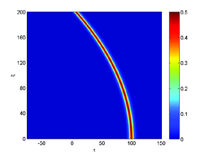
Figure 8: Evolution of pulse solutions, $|q|$ with (a) peak amplitude equal to 0.5 for $\chi=0.1$ and $P_{\text{th}}=0.2$ and (b) peak amplitude equal to 0.3 for $\chi=0.2$ and $P_{\text{th}}=0$. We have used $\sigma=1$.

Figure 9: Input and output for the simulation whose contour is on Fig. 8.

Finally, let us return to the physical variables and calculate the actual acceleration and frequency shift. The adimensional acceleration $a$ does not correspond directly to an acceleration in physical units, nevertheless let us define the acceleration $a_{r}$ as the second derivative of the temporal peak position in the group velocity reference frame relatively to the propagation distance $z$, namely

$$a_{r}=\frac{d^{2}t_{\text{peak}}}{dz^{2}}=\frac{|\beta_{2}|^{2}}{t_{0}^{3}}\frac{d^{2}\tau_{\text{peak}}}{d\xi^{2}}=-\frac{|\beta_{2}|^{2}}{t_{0}^{3}}\frac{a}{2}=-\frac{A_{\text{eff}}^{3}\gamma^{3}}{2\tilde{\sigma}^{3}|\beta_{2}|}\alpha(\chi,P_{\text{th}},P_{\text{peak}})$$

Note that the negative signal only implies that the pulse is traveling toward negative $t$ but since $t$ is measured in a reference frame that travels with the group velocity for $\omega_{0}$, the pulse is gaining velocity whenever this acceleration is negative. This change in velocity is due to a deviation in frequency that is linear with the distance $z$, as expressed in the phase (4), and given by

$$\Delta\omega=-\frac{d\theta}{dt}=-\frac{a_{r}}{|\beta_{2}|}z$$

Since equation (3) neglects the photoionization related losses that are small for pulses whose peak amplitude is comparable with the threshold, for $\chi$ not too large, we may use expression (8) for $\alpha$ and approximate the frequency approximated by

$$\Delta\omega=-\frac{8}{15}\frac{t_{R}\gamma^{2}}{|\beta_{2}|}\psi_{\text{peak}}^{4}z+\frac{k_{0}(\omega_{T}/\omega_{0})^{2}\tilde{\sigma}}{3A_{\text{eff}}}\frac{\left(\psi_{\text{peak}}^{2}-\psi_{\text{th}}^{2}\right)^{3/2}}{\psi_{\text{peak}}}z$$

which gives the standard result for the IRS Gordon (1986); Facão et al. (2010) and the effect of plasma growing with order $\psi_{\text{peak}}^{2}$.

V Conclusions

We have found the self-similar accelerating solutions of a generalized NLS that includes IRS and a term for plasma induced nonlinearity. This equation models the propagation of pulses in gas filled HC-PCFs where it has occurred photoionization of the gas. The solutions are very close to the NLS sech soliton as long as the strength of the plasma term is relatively low and the solution amplitude is relatively large. The accelerations and the blueshifting increase with the peak amplitude of the pulses. In case of pulse solutions whose peak intensity is close to the photoionization threshold, which are the ones for which the equation better models the physical effects, the frequency blueshift increases in the same order as the square of peak amplitude. However, also the same solutions, whose peak amplitudes are close to the threshold, may exhibit a profile that is considerably different from the sech, have long tails and decay along the propagation distance.