A Matrix Framework for the Solution of ODEs:
Initial-, Boundary-, and Inner-Value Problems

Abstract

A matrix framework is presented for the solution of ODEs, including initial-, boundary and inner-value problems. The framework enables the solution of the ODEs for arbitrary nodes. There are four key issues involved in the formulation of the framework: the use of a Lanczos process with complete reorthogonalization for the synthesis of discrete orthonormal polynomials (DOP) orthogonal over arbitrary nodes within the unit circle on the complex plane; a consistent definition of a local differentiating matrix which implements a uniform degree of approximation over the complete support — this is particularly important for initial and boundary value problems; a method of computing a set of constraints as a constraining matrix and a method to generate orthonormal admissible functions from the constraints and a DOP matrix; the formulation of the solution to the ODEs as a least squares problem. The computation of the solution is a direct matrix method. The worst case maximum number of computations required to obtain the solution is known a-priori. This makes the method, by definition, suitable for real-time applications.

The functionality of the framework is demonstrated using a selection of initial value problems, Sturm-Liouville problems and a classical Engineering boundary value problem. The framework is, however, generally formulated and is applicable to countless differential equation problems.

1 Introduction

There are a number of papers in which the Taylor Matrix is used to compute solutions to differential equations [11, 14]. These methods use the known analytical relationship between the coefficients $\boldsymbol{s}$ of a Taylor polynomial and those of its derivatives $\dot{\boldsymbol{s}}$ to compute a differentiating matrix $\mathsf{D}$. The matrix $\mathsf{D}$ together with the matrix of basis functions arranged as the columns of the matrix $\mathsf{B}$ are used to compute numerical solutions to the differential equations. The method of the Taylor matrix was also extended to the computation of fractional derivatives [12]. The problem associated with this approach is that the computation of the numerical solutions requires the inversion of the Vandermonde matrix, a process which is known to be numerically unstable, and dependent on the degree and node placement. The advantage of the Taylor approach lies in its ability to yield a solution for arbitrary nodes.

A Chebyshev matrix approach was presented by Sezer [26]. The approach is fundamentally the same as for the Taylor matrix, whereby the Chebyshev polynomials are used as an alternative to the geometric polynomials. The main restriction associated with the Chebvshev polynomial approach is that the numerical solution to the differential equations is restricted to the locations of the Chebyshev points; this lacks the generality needed for many differential equations and applications.

Podlubny introduced a matrix approach to discrete fractional calculus [20] and later extended this work to partial fractional differential calculus [22, 21]. Triangular strip matrices play a central role in the work; they are used to perform integration. They implement the integration from a lower to an upper bound (or vice versa), whereby the errors accumulate as the integration proceeds. This poses a problem if inverse problems are addressed, since it gives the solution an implicit direction and a different accumulation of errors if the problem is solved from lower to upper bound or from upper to lower. Furthermore, it is assumed that the initial value is zero. This makes the method unsuitable for arbitrary boundary conditions. An early source of this formulation was proposed by Courant et al. [5], (a later English translation of the paper is available [6]).

A matrix solution specific to Sturm-Liouville problems was presented by Amodio [2]. The method is specifically restricted to Sturm-Liouville problems; furthermore, it only supports solutions on regularly spaced nodes. The results are correspondingly modest for problems where the Chebyshev points yield better solutions, e.g., in the solution of the truncated hydrogen equation. A number of matrix approaches based on the Numerov method, and modifications of this method, have also been presented [15] for the solution of Sturm-Liouville problems, however, these methods can not be extended to ODEs in general.

In this paper we formulate a general matrix framework for the solution of ordinary differential equations, with arbitrary initial-, boundary-, or inner values. the main contributions of the paper are:

1. The proposal of a consistent framework of matrices and solution approaches which can be applied to initial-, boundary-, and inner-value problems;

2. The implementation of new approached to the synthesis of discrete orthonormal basis functions, with and without weighting;

3. Generating differentiating matrices which are of constant degree of approximation over the complete support. It is particularly important that the degree of approximation is consistent at the ends of the support if initial and boundary value problems are to be solved satisfactorily;

4. The derivation of a means of synthesizing constrained basis functions which form orthonormal matrices. This basis functions span the space of all solutions which fulfil the constraints. They can be used as admissible functions in a discrete equivalent of a Rayleigh-Ritz method;

5. The formulation of the solution of the ODEs as least squares approximations. In this manner there is no accumulation of errors.

This paper is structured as follows: In Section (2) the framework for the generation of all the matrices required to formulate differential equations as matrix linear differential operators is presented. Section (3) presents the approach to discretization of the differential equations and their solution as a least squares minimization is presented. The required conditions for a unique solution are derived and two solution approaches are presented: a direct solution in the case of a unique solution and the implementation of a discrete Rayleigh-Ritz method for eigenvalue/eigenvector solutions, e.g., as encountered in the solution of Sturm-Liouville problems.. Finally, in Section (4) the performance of the proposed framework is tested with a series of initial-value problems, Sturm-Liouville problems and a classical Engineering boundary value problem.

2 Algebraic Framework

In this section we derive the structure and methods for the synthesis of all matrices required for the discretization and solution of ordinary differential equations.

2.1 Quality Measure for Basis Functions

An objective measure for the quality of a set of basis functions is required if the sources of numerical error are to be determined and the best synthesis method is to be selected. In this paper continuous polynomials are considered which form orthogonal bases when evaluated over a discrete measure. The basis functions $\boldsymbol{b}_{i}$, i.e., the polynomials evaluated at discrete points, can be concatenated to form a matrix, $\mathsf{B}=[\boldsymbol{b}_{1}\ldots\boldsymbol{b}_{n}]$. The discrete orthogonal polynomials (DOP) are characterized by the relationship,

$$\mathsf{B}^{\textrm{T}}\,\mathsf{W}\,\mathsf{B}=\mathsf{I},$$ (1)

where $\mathsf{W}$ is the weighting matrix. The Gram matrix is defined as $\mathsf{G}\triangleq\mathsf{B}^{\textrm{T}}\,\mathsf{W}\,\mathsf{B}$. Consequently, the orthogonal complement $\mathsf{G}^{\perp}\triangleq\mathsf{I}-\mathsf{B}^{\textrm{T}}\,\mathsf{W}\,\mathsf{B}=\mathsf{0}$ should be a matrix containing only zeros. However, this is not the case, due to the loss of orthogonality in the three term relationship resulting from numerical errors. These numerical errors determine the quality of the basis functions and for which we require a measure. The determinant of $\mathsf{G}$ has in the past been used as a measure for the quality $\epsilon_{g}=\mathrm{det}\,\mathsf{G}$ of the basis functions. However, this measure does not yield stable estimates [8, Chapter 2, Sec. 2.7.3]. We propose the Frobenius norm of $\mathsf{G}^{\perp}$ as an error measure, i.e., $\epsilon_{F}=\|\mathsf{G}^{\perp}\|_{F}$, this is the sum of the square of all errors w.r.t. the orthogonality of the basis functions, $\epsilon_{F}\geq 0$. This is a posteriori measure, i.e., we compute the basis functions and then determine their quality. Wilkinson [27] points out that a-priory prediction of error bounds yield unreliable results and a posteriori analysis is preferred. The numerical results obtained for different synthesis procedures can be found in Section (4.1).

2.2 Numerically Stable Synthesis of Basis Functions and their Derivatives

Gram [9] proposed what is now known as the Gram-Schmidt orthogonalization process to generate polynomials [4]. The Gram-Schmidt process is, however, numerically unstable [8, Chapter 5] and errors accumulate as the number of integrations increases, i.e., with increasing polynomial degree. This precludes the synthesis of polynomials of higher degree with this method. Considerable research has been performed on discrete polynomials and their synthesis [16, 29, 30, 28, 10, 31, 32, 3]. The research was primarily in conjunction with the computation of moments for image processing. None of these papers present a method which is capable of synthesizing discrete orthogonal polynomials of high quality for arbitrary nodes located within the unit circle on the complex plane.

Here it is proposed to synthesize the polynomial basis functions using a Lanczos process with complete reorthogonalization [8, Chapter 9, p. 482],[17]. The procedure can be summarized as follows: Given a vector $\boldsymbol{x}$ of $n$ nodes with mean $\bar{x}$, i.e., the points at which the differential equation is to be solved: first compute the two basis functions $\boldsymbol{b}_{0}$, $\boldsymbol{b}_{1}$ and initialize the matrix of basis functions $\mathsf{B}$,

$$\boldsymbol{b}_{0}=\boldsymbol{1}/\sqrt{n}\hskip 28.45274pt\boldsymbol{b}_{1}=\frac{\boldsymbol{x}-\bar{x}}{\mathop{\|}\boldsymbol{x}-\bar{x}\mathop{\|}_{2}}\hskip 28.45274pt\text{and}\hskip 28.45274pt\mathsf{B}=\left[\boldsymbol{b}_{0},\boldsymbol{b}_{1}\right].$$ (2)

The remaining polynomials are synthesized by repeatedly performing the following computations:

1. Compute the polynomial of the next higher degree,

   $$\boldsymbol{b}_{n}=\boldsymbol{b}_{1}\circ\boldsymbol{b}_{n-1};$$ (3)

2. perform a complete reorthogonalization,

   $$\boldsymbol{b}_{n} =\boldsymbol{b}_{n}-\mathsf{B}\,\mathsf{B}^{\textrm{T}}\,\boldsymbol{b}_{n}$$ (4)

   $$=\left\{\mathsf{I}-\mathsf{B}\,\mathsf{B}^{\textrm{T}}\right\}\boldsymbol{b}_{n}$$ (5)

   by projection onto the orthogonal complement of all previously synthesized polynomials. It is important to note that the reorthogonalization is w.r.t. to the complete set of basis functions, not just the previous polynomial.

3. Normalize the vector,

   $$\boldsymbol{b}_{n}=\frac{\boldsymbol{b}_{n}}{\mathop{\|}\boldsymbol{b}_{n}\mathop{\|}_{2}},$$ (6)

4. and augment the matrix of basis functions,

   $$\mathsf{B}=\left[\mathsf{B},\boldsymbol{b}_{n}\right].$$ (7)

This procedure yields a set of orthonormal polynomials from a set of arbitrary nodes located within the unit circle on the complex plane. Although in [7] the Lanczos process is used to compute discrete orthogonal polynomials, the authors seem to have overseen the possibility (necessity) of using complete reorthogonalization at each step of the polynomial synthesis.

By taking the derivative of the recurrence relationship w.r.t. $x$, we obtain the equations required to simultaneously synthesize the differentials of the polynomials. This procedure appears in [13] for the Legendre and Chebyshev polynomials. Here the method is generalized to the synthesis of polynomials from arbitrary nodes. With this, the synthesis procedure delivers a set of orthonormal basis functions $\mathsf{B}$ and their derivatives $\dot{\mathsf{B}}$.

2.3 Weighted Basis Functions

A set of discrete basis functions in matrix form, $\mathsf{B}_{w}$ are orthogonal with respect to a weighting matrix $\mathsf{W}$ if,

$$\mathsf{B}^{\textrm{T}}_{w}\mathsf{W}\mathsf{B}_{w}=\mathsf{I}.$$ (8)

In the case of a weighting function $w(x)$ the weighting matrix is given by $\mathsf{W}=\mathop{\operator@font diag}\nolimits\left\{{w(x_{1})\ldots w(x_{n})}\right\}$. Given a set of orthonormal basis functions $\mathsf{B}$ and a positive definite weighting matrix $\mathsf{W}$, there exists a set of weighted basis functions $\mathsf{B}_{w}$, such that $\mathsf{B}_{w}=\mathsf{B}\,\mathsf{U}$, whereby $\mathsf{U}$ is a full rank upper triangular matrix. Substituting into Equation (8) yields,

$$\mathsf{U}^{\textrm{T}}\,\mathsf{B}^{\textrm{T}}\,\mathsf{W}\,\mathsf{B}\,\mathsf{U}=\mathsf{I}.$$ (9)

Since $\mathsf{U}$ is full rank, we may invert it to obtain,

$$\mathsf{B}^{\textrm{T}}\,\mathsf{W}\,\mathsf{B}=\mathsf{U}^{-\textrm{T}}\,\mathsf{U}^{-1}.$$ (10)

The Cholesky decomposition $\mathop{\mathrm{chol}}\left\{\mathsf{A}\right\}$ of a matrix exists and is unique such that $\mathsf{A}=\mathsf{G}\,\mathsf{G}^{\textrm{T}}$ if $\mathsf{A}$ is real positive definite. The matrix $\mathsf{G}$ is a full rank lower triangular matrix. Consequently, the Cholesky decomposition $\mathop{\mathrm{chol}}\left\{\mathsf{B}^{\textrm{T}}\,\mathsf{W}\,\mathsf{B}\right\}$ exists if $\mathsf{W}$ is real positive definite, since $\mathsf{B}$ is orthonormal. Applying the decomposition yields,

$$\mathsf{B}^{\textrm{T}}\,\mathsf{W}\,\mathsf{B}=\mathsf{G}\,\mathsf{G}^{\textrm{T}}=\mathsf{U}^{-\textrm{T}}\,\mathsf{U}^{-1}.$$ (11)

The sought matrix $\mathsf{U}$ is clearly given by,

$$\mathsf{U}=\mathsf{G}^{-\textrm{T}}.$$ (12)

With this the weighted basis functions are fully defined. The condition number of the basis functions depends soley on the condition number of the weighting matrix $\mathsf{W}$. In the case where the weighting matrix is derived from a weighting function $w(x)$, the condition number is determined by the extreme values of $w(x)$.

2.4 Differentiating Matrices

There are both global [11, 14, 12, 26, 13] and local [5, 25, 6, 20, 22] approaches to computing discrete estimates for derivatives. Global methods proposed in the past have used the known relationship between the coefficients of a polynomial and the coefficients of the derivative of the polynomial to compute a differentiating matrix.

The computation of a differentiating matrix from polynomial bases proceeds as follows: The spectrum of the signal $\boldsymbol{y}$ with respect to the basis functions $\mathsf{B}$ is computed as,

$$\boldsymbol{s}=\mathsf{B}^{+}\,\boldsymbol{y}.$$ (13)

For example, $\mathsf{B}$ may be the Vandermonde matrix; this is case with Taylor methods [11, 14, 12]. The relationship between the spectrum $\boldsymbol{s}$ and the spectrum of the derivatives is given by,

$$\dot{\boldsymbol{s}}=\mathsf{M}\,\boldsymbol{s}\hskip 56.9055pt\text{whereby}\hskip 56.9055pt\mathsf{M}=\begin{bmatrix}0&1&0&\ldots&0\\ 0&0&2&\ldots&0\\ 0&0&0&\ddots&0\\ 0&0&0&\ldots&n\\ 0&0&0&\ldots&0\end{bmatrix}.$$ (14)

Consequently,

$$\dot{\boldsymbol{y}}=\mathsf{B}\,\mathsf{M}\,\mathsf{B}^{+}\,\boldsymbol{y}=\mathsf{D}\,\boldsymbol{y}.$$ (15)

That is, the differentiating matrix is computed as, $\mathsf{D}=\mathsf{B}\,\mathsf{M}\,\mathsf{B}^{+}$. In the case of the Taylor (Vandermonde) matrix this involves computing the pseudo-inverse of the Vandermonde matrix: with all the associated numerical problems. In the case of the Chebyshev polynomials [26, 13] $\mathsf{B}^{+}=\mathsf{B}^{\textrm{T}}$ and a different matrix $\mathsf{M}$ is required, see [26] for details. The method is not appropriate if arbitrary nodes are required, e.g. this may be required if the framework is to be used to solve the problems associated with monitoring mechanical structures [19]. The advantage of Global methods is that they deliver a differentiating matrix which is valid for the complete support.

The solution chosen here is to compute $\mathsf{D}$ form the basis functions and their derivatives, i.e., given $\dot{\mathsf{B}}$ and $\mathsf{B}$ an appropriate derivative operator, $\mathsf{D}$, should have the property that,

$$\mathsf{D}\,\mathsf{B}=\dot{\mathsf{B}}.$$ (16)

Post-multiplying by $\mathsf{B}^{\textrm{T}}$ yields

$$\mathsf{D}_{B}\triangleq\mathsf{D}\,\mathsf{B}\,\mathsf{B}^{\textrm{T}}=\dot{\mathsf{B}}\,\mathsf{B}^{\textrm{T}}.$$ (17)

If the basis function set is complete, i.e., $\mathsf{B}\,\mathsf{B}^{\textrm{T}}$ then the above equation yields the differentiating matrix directly,

$$\mathsf{D}=\dot{\mathsf{B}}\,\mathsf{B}^{\textrm{T}}.$$ (18)

This computation is valid for arbitrary nodes. If a truncated, i.e., an incomplete, set of basis functions is used then $\mathsf{B}\,\mathsf{B}^{\textrm{T}}$ is the projection onto the the basis functions $\mathsf{B}$ and $\mathsf{D}_{B}$ is then a regularizing differentiating matrix. The matrix $\mathsf{D}_{B}$ can be applied to the computation of estimates for derivatives in the presence of noise.

A differentiating matrix should be rank-1 deficient; it should have the constant vector as its null space, i.e., $\mathsf{D}\,\boldsymbol{1}\,\alpha=\boldsymbol{0}$. The properties of the $\mathsf{D}$ are, however, dependent on the nodes being used, e.g. the Chebyshev nodes permit global differentiating matrices for very high degrees. With other sets of nodes the condition number of a differentiating matrix can increase with the degree of the polynomial being used. At some point the matrix starts to have additional null spaces, which are associated with numerical errors occuring due to insufficient numerical precision, this effect is shown in Figure (1) for the Gram polynomials.

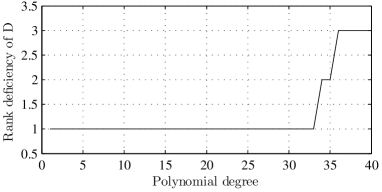
Fig. 1: Rank deficiency of the differentiating matrix $\mathsf{D}$ as a function of the degree of a Gram polynomial, when $\mathsf{D}$ is synthesized using Equation (18).

Once the condition number of a global differentiating matrix has degenerated below an acceptable level, it becomes necessary to compute local approximations [25, 18]. Courant [5, 6] proposed, in $1927$, using both forward and backward differences to compute estimates for the first derivative. The method has also been used in [20, 22] to this end. More commonly the tri-diagonal matrix, shown here for $6$ points,

$$\mathsf{D}_{t}=\frac{1}{h}\begin{bmatrix}-1&1&0&0&0&0\\ -0.5&0&0.5&0&0&0\\ 0&-0.5&0&0.5&0&0\\ 0&0&-0.5&0&0.5&0\\ 0&0&0&-0.5&0&0.5\\ 0&0&0&0&-1&1\end{bmatrix}$$ (19)

is used to compute a discrete local estimate for the first differential. This operator is only of degree $d=2$ accurate in the core of the approximation and at both ends of the support only of degree $d=1$ accurate. This makes this discrete operator unsuitable for the computation of derivatives at the end of the support, as is required for BVPs and IVPs. It is also not suitable for systems whose solutions are locally of degree higher than $d>2$. Furthermore, this operators assumes equally spaced nodes. In [2] higher order finite difference schemes are proposed with end-point formulas. However, only equidistant spaced nodes are considered. For example, the appropriate three point operator for the Gram $\mathsf{D}_{G,3}$ and for the Chebyshev $\mathsf{D}_{C,3}$ nodes, are,

$$\mathsf{D}_{G,3}=\begin{bmatrix}-4.5&6&-1.5&0&0&0\\ -1.5&0&1.5&0&0&0\\ 0&-1.5&0&1.5&0&0\\ 0&0&-1.5&0&1.5&0\\ 0&0&0&-1.5&0&1.5\\ 0&0&0&1.5&-6&4.5\end{bmatrix}$$ (20)

and

$$\mathsf{D}_{C,3}=\begin{bmatrix}-5.2779&6.0944&-0.8165&0&0&0\\ -2.4495&1.633&0.8165&0&0&0\\ 0&-1.1954&0.29886&0.89658&0&0\\ 0&0&-0.89658&-0.29886&1.1954&0\\ 0&0&0&-0.8165&-1.633&2.4495\\ 0&0&0&0.8165&-6.0944&5.2779\end{bmatrix},$$ (21)

both computed for $n=6$ points in the interval $-1<x<1$. Note the three points formulas at both ends of the support.

In keeping with the formulation of the basis functions for arbitrary nodes: the method for local differential approximation is also formulated here for arbitrary nodes. A generalized formulation of local differentiating matrix requires the vector $\boldsymbol{x}$ of $n$ arbitrarily placed nodes, the support length $l_{s}$ and the degree $d$ of the approximation. Only odd support lengths are considered here, to avoid the need for forward and backward formulas. It is convenient to define the support length $l_{s}=2w_{s}+1$ in terms of the half-width $w_{s}$. The vector $\boldsymbol{x}$ of nodes is segmented into $m=n-2w_{s}$ overlapping segments, for each segment,

$$\boldsymbol{s}(i)=\boldsymbol{x}(i-w_{s}:i+w_{s})\hskip 28.45274pt\forall\,i\in[w_{s}+1,n-w_{s}]$$ (22)

a local set of basis functions $\mathsf{B}_{s}$ and derivatives of the basis functions $\dot{\mathsf{B}}_{s}$ are computed. Then the differentiating matrix associated with the segment is determined $\mathsf{D}_{s}=\dot{\mathsf{B}}_{s}\,\mathsf{B}^{\textrm{T}}_{s}$. The first and last segments yield the end-point formulas as required. The remaining segment yields the required central formula of coefficients to locally approximate the derivative. Clearly, for the inner-segments it is only necessary to compute the center row vector of the local differentiating operator $\mathsf{D}_{s}$. The use of approximating or interpolating polynomials leads to the generation of differentiating matrices with and without regularization respectively. The Wilkinson diagram for the general structure of a local differentiating matrix $\mathsf{D}_{L}$ is shown in Equation (23) for the example of $l_{s}=5$ and $n=10$. The specific entries in the matrix are a function of the spacing of the nodes.

$$\mathsf{D}_{5}=\begin{bmatrix}\times&\times&\times&\times&\times&0&0&0&0&0\\ \times&\times&\times&\times&\times&0&0&0&0&0\\ \hline\cr\times&\times&\times&\times&\times&0&0&0&0&0\\ 0&\times&\times&\times&\times&\times&0&0&0&0\\ 0&0&\times&\times&\times&\times&\times&0&0&0\\ 0&0&0&\times&\times&\times&\times&\times&0&0\\ 0&0&0&0&\times&\times&\times&\times&\times&0\\ 0&0&0&0&0&\times&\times&\times&\times&\times\\ \hline\cr 0&0&0&0&0&\times&\times&\times&\times&\times\\ 0&0&0&0&0&\times&\times&\times&\times&\times\end{bmatrix}$$ (23)

All computations of the local derivative are of length $l_{s}$ and of constant approximation degree $d_{a}=2w_{s}$ over the complete support. This is important if derivatives are to be computed at the ends of the support; furthermore, errors at the end of the support associated with inconsistent approximations will propagate through the entire solution when $\mathsf{D}$ is being used in the solution of differential equations. This procedure proposed here delivers a local differentiating matrix for arbitrary nodes.

2.5 Defining Constraints

In Section (2.4) it was shown that a discrete approximation to differentiation can be computed as a linear matrix operator. Consequently, both differential and integral constraints are linear. In the framework proposed here, a constraint is implemented by restricting a linear combination $\boldsymbol{c}^{\textrm{T}}\,\boldsymbol{y}$ of the solution vector $\boldsymbol{y}$ to have a scalar value $d$, i.e.,

$$\boldsymbol{c}^{\textrm{T}}\,\boldsymbol{y}=d.$$ (24)

This is a very general mechanism, since any constraining function can be implemented at a point $x_{i}$ for which a linear $n$ point expansion around this point exists. To give an example, consider the $C^{2}$ continuous periodicity constraint $y(0)=y(1)$, $\dot{y}(0)=\dot{y}(1)$ and $\ddot{y}(0)=\ddot{y}(1)$: given the differentiating matrix $\mathsf{D}$ and $\mathsf{D}^{2}$, the three constraints can be formulated as:

$$[1,0,\ldots,0,-1]\,\boldsymbol{y}=\boldsymbol{c}^{\textrm{T}}_{1}\,\boldsymbol{y} =0,$$ (25)

$$\left\{\mathsf{D}(1,:)-\mathsf{D}(end,:)\right\}\,\boldsymbol{y}=\boldsymbol{c}^{\textrm{T}}_{2}\,\boldsymbol{y} =0,$$ (26)

$$\left\{\mathsf{D}^{2}(1,:)-\mathsf{D}^{2}(end,:)\right\}\,\boldsymbol{y}=\boldsymbol{c}^{\textrm{T}}_{3}\,\boldsymbol{y} =0.$$ (27)

Given a set of $m$ constraints, the constraining vectors $\boldsymbol{c}_{i}$ are concatenated to form the matrix $\mathsf{C}=[\boldsymbol{c}_{1}\ldots\boldsymbol{c}_{m}]$ and the corresponding scalars $d_{i}$ form the vector $\boldsymbol{d}^{\textrm{T}}=[d_{1}\ldots d_{m}]$, so that,

$$\mathsf{C}\,\boldsymbol{y}=\boldsymbol{d}.$$ (28)

2.6 Homogeneously Constrained Admissible Functions

Starting from a set of basis functions $\mathsf{B}$ such that $\mathsf{B}^{\textrm{T}}\,\mathsf{W}\,\mathsf{B}=\mathsf{I}$, we wish to derive a method of synthesizing a set of constrained basis functions $\mathsf{B}_{c}$ which fulfil the conditions:

$$\mathsf{B}^{\textrm{T}}_{c}\,\mathsf{W}\,\mathsf{B}_{c}=\mathsf{I},\hskip 28.45274pt\mathsf{C}^{\textrm{T}}\,\mathsf{B}_{c}=\boldsymbol{0}\hskip 28.45274pt\text{and}\hskip 28.45274pt\mathsf{B}_{c}=\mathsf{B}\,\mathsf{X},$$ (29)

i.e., the constrained basis functions form an orthonormal basis set with respect to the weighting matrix $\mathsf{W}$. If $\mathsf{B}$ is orthonormal, i.e., $\mathsf{B}^{\textrm{T}}\,\mathsf{B}=\mathsf{I}$ then so is $\mathsf{B}_{c}$. The constrained basis functions fulfil the homogeneous constraints defined by $\mathsf{C}$. If $\mathsf{B}$ is complete then it spans the complete $n\times n$ space, given $p=\mathop{\operator@font rank}\nolimits{(\mathsf{C})}$, i.e., the number of independent constraints, $\mathsf{B}_{c}$ is of dimension $n\times(n-p)$ and spans the complete space in which the constraints are fulfilled. Consequently, all possible vectors $\boldsymbol{y}$ which fulfil the constraints are given by,

$$\boldsymbol{y}=\mathsf{B}_{c}\,\boldsymbol{\alpha}$$ (30)

where $\boldsymbol{\alpha}$ is an $n-p$ vector.

A solution to the task of determining $\mathsf{X}$ was presented in [19]; however, a more succinct derivation is provided here. The conditions from Equation (29) require,

$$\mathsf{C}^{\textrm{T}}\,\mathsf{B}\,\mathsf{X}=\boldsymbol{0}$$ (31)

and with this $\mathsf{X}$ must lie in the null space of $\mathsf{C}^{\textrm{T}}\,\mathsf{B}$. Applying QR decomposition to $\mathsf{B}^{\textrm{T}}\,\mathsf{C}$ yields,

$$\mathsf{Q}\,\mathsf{R}=\mathsf{B}^{\textrm{T}}\,\mathsf{C},$$ (32)

and consequently,

$$\mathsf{X}^{\textrm{T}}\,\mathsf{Q}\,\mathsf{R}=\boldsymbol{0}$$ (33)

The matrices $\mathsf{Q}$ and $\mathsf{R}$ are partitioned according to the span and null space of $\mathsf{B}^{\textrm{T}}\,\mathsf{C}$,

$$\mathsf{Q}=[\mathsf{Q}_{s},\mathsf{Q}_{n}]\hskip 28.45274pt\text{and}\hskip 28.45274pt\mathsf{R}=\begin{bmatrix}\mathsf{R}_{s}\\ \mathsf{0}\end{bmatrix}.,$$ (34)

with $\mathsf{R}_{s}$ of dimension $p\times p$. The $n\times p$ matrix $\mathsf{Q}_{s}$ forms a basis set for the span and the $n\times(n-p)$ matrix $\mathsf{Q}_{n}$ forms a basis set for the null space of $\mathsf{B}^{\textrm{T}}\,\mathsf{C}$. Consequently,

$$\mathsf{X}^{\textrm{T}}\,\mathsf{Q}_{s}=\mathsf{0}\hskip 28.45274pt\text{and}\hskip 28.45274pt\left(\mathsf{\mathsf{X}^{\textrm{T}}\,\mathsf{Q}_{n}}\right)^{\textrm{T}}\mathsf{W}\,\mathsf{X}^{\textrm{T}}\,\mathsf{Q}_{n}=\mathsf{I}.$$ (35)

Now applying an RQ decomposition to $\mathsf{Q}_{n}$ yields,

$$\hat{\mathsf{R}}\,\hat{\mathsf{Q}}_{n}=\mathsf{Q}_{n}.$$ (36)

$\hat{\mathsf{R}}$ is orthonormal, since both $\hat{\mathsf{Q}}_{n}$ and $\mathsf{Q}_{n}$ are by definition orthonormal. Now, selecting $\mathsf{X}=\hat{\mathsf{R}}$ yields $\mathsf{X}^{\textrm{T}}\,\hat{\mathsf{R}}\,\hat{\mathsf{Q}}_{n}=\hat{\mathsf{Q}}_{n}$, and with this all the conditions from Equation (29) are fulfilled. The matrix $\mathsf{X}$ being orthonormal ensures that $\mathsf{B}_{c}$ fulfils the same orthonormal condition as does $\mathsf{B}$. Furthermore, $\mathsf{X}$ has an implicit partitioning,

$$\mathsf{X}=\begin{bmatrix}\mathsf{X}_{1}\\ \mathsf{X}_{2}\end{bmatrix}$$ (37)

whereby, $\mathsf{X}_{1}$ is a $p\times(n-p)$ block matrix and $\mathsf{X}_{2}$ is a $(n-p)\times(n-p)$ upper triangular matrix. This structure ensures that the number of roots in the constrained basis functions $\mathsf{B}_{c}$ is ordered in the same manner as in $\mathsf{B}$.

3 Discretizing and Solving Ordinary Differential Equations

In the previous section all the matrices required for the discretization of ordinary differential equations were derived. In this section the discretization of initial-, boundary- and inner value problems is presented together with the associated methods of solving the resulting matrix equations.

3.1 Initial Value Problems

In this paper we are considering the solution of linear ordinary differential equations with constant or variable coefficients, they can in general be formulated as,

$$p_{k}(x)\,y^{(k)}(x)\ldots+p_{1}(x)\,y^{(1)}(x)+p_{0}(x)\,y(x)=g(x)$$ (38)

to which a set of $k$ constraints are required to ensure a unique solution. The term $y^{(k)}(x)$ represents the $k^{\text{th}}$ derivative of $y(x)$. Given the matrices derived previously, the discretization of Equation (38) is direct and simple, each term $p_{k}(x)\,y^{(k)}(x)$ is dicreteized as follows: The matrix $\mathsf{P}_{k}$ is formed such that $\mathsf{P}_{k}=\mathop{\operator@font diag}\nolimits{\left\{p_{k}(\boldsymbol{x})\right\}}$, whereby $p_{k}(\boldsymbol{x})$ is the vector of values obtained by evaluating the function $p_{n}(x)$ at the vector of points $\boldsymbol{x}$; the term $y^{(k)}(x)$ is discretized as $\mathsf{D}^{k}\,\boldsymbol{y}$, i.e., the $k^{\text{th}}$ power of $\mathsf{D}$, which is the differentiating matrix derived in Section (2.4). Summarizing, each term is discretized as follows,

$$p_{k}(x)\,y^{(k)}(x)\rightarrow\mathsf{P}_{k}\,\mathsf{D}^{k}\,\boldsymbol{y}.$$ (39)

and the vector $\boldsymbol{g}=g(\boldsymbol{x})$. Applying this to all terms in Equation (38) yields,

$$\mathsf{P}_{k}\,\mathsf{D}^{k}\,\boldsymbol{y}\ldots+\mathsf{P}_{1}\,\mathsf{D}\,\boldsymbol{y}+\mathsf{P}_{0}\,\boldsymbol{y}=\boldsymbol{g}$$ (40)

The matrix equivalent of the linear differential operator $\mathsf{L}$ is now defined as,

$$\mathsf{L}\triangleq\mathsf{P}_{k}\,\mathsf{D}^{k}\ldots+\mathsf{P}_{1}\,\mathsf{D}+\mathsf{P}_{0},$$ (41)

and the set of $k$ constraints are implemented as defined in Section (2.5), yielding

$$\mathsf{L}\,\boldsymbol{y}=\boldsymbol{g}\hskip 28.45274pt\text{given}\hskip 28.45274pt\mathsf{C}^{\textrm{T}}\,\boldsymbol{y}=\boldsymbol{d}.$$ (42)

the matrix $\mathsf{C}$ has the dimension $n\times k$.

A unique solution to the ODE exists only if

$$\mathop{\operator@font rank}\nolimits{\begin{bmatrix}\mathsf{L}\\ \mathsf{C}^{\textrm{T}}\end{bmatrix}}=n$$ (43)

i.e., the linear differential operator and the constraints must form a full rank system of equations. There are many Engineering application where this is not the case, e.g. the equations for the vibration of a beam, and Sturm-Liouville problems. A different solution approach is proposed for this class of problems in Section (3.2).

3.1.1 Solution as a constrained least squares problem

The formulation of determining $\boldsymbol{y}$ from Equation (42) as the solution of a least squares minimization problem yields,

$$\min_{y}\|\mathsf{L}\,\boldsymbol{y}-\boldsymbol{g}\|_{2}^{2}\hskip 28.45274pt\text{given}\hskip 28.45274pt\mathsf{C}^{\textrm{T}}\,\boldsymbol{y}=\boldsymbol{d}.$$ (44)

This is the well known problem of least squares with equality constraints (LSE). Efficient and accurate solutions can be found in [8, Chapter 12]. This method will yield solutions for ODEs with consistent constraints and a least squares solution in the case of over-constrained systems and perturbed systems. It is not a suitable approach for Sturm-Liouville type problems.

The worst case number of floating point operations (FLOPS) required to perform the computation is known a-priori. This, by definition, makes the method suitable for real time applications.

3.1.2 Spectral Reqularization

Spectral regularization is introduced here to limit the number of zeros in the basis functions and with this to reduce the errors associated with aliasing. Assuming $\boldsymbol{y}$ can be sufficiently accurately approximated by a series of $r$ orthonormal basis functions, we may write,

$$\boldsymbol{y}=\mathsf{B}_{r}\,\boldsymbol{\alpha},$$ (45)

whereby $\mathsf{B}_{r}=\mathsf{B}(:,1\ldots r)$. Now defining $\mathsf{L}_{r}\triangleq\mathsf{L}\,\mathsf{B}_{r}$ and $\mathsf{C}_{r}\triangleq\mathsf{B}^{\textrm{T}}_{r}\,\mathsf{C}$, and substituting into Equation (44) yields,

$$\min_{\boldsymbol{\alpha}}\|\mathsf{L}_{r}\,\boldsymbol{\alpha}-\boldsymbol{g}\|_{2}^{2}\hskip 28.45274pt\text{given}\hskip 28.45274pt\mathsf{C}^{\textrm{T}}_{r}\,\boldsymbol{\alpha}=\boldsymbol{d},$$ (46)

whereby the series coefficients $\boldsymbol{\alpha}$ are to be determined. In addition to introducing regularization, the truncated basis functions also reduce the size of the LS problem to be solved.

3.1.3 Solution of Homogeneously Constrained IVPs

Homogeneously Constrained IVPs for a special subclass of problems for which there is a particularly simple solution. Let the solution $\boldsymbol{y}$ be a linear combination of a set of constrained basis functions, i.e., $\boldsymbol{y}=\mathsf{B}_{c}\,\boldsymbol{\alpha}$, which fulfil the homogeneous constraints $\mathsf{C}^{\textrm{T}}\,\mathsf{B}_{c}=0$ associated with the IVP. Equation (44) now simplifies to the unconstrained least squares problem,

$$\min_{\boldsymbol{\alpha}}\|\mathsf{L}\,\mathsf{B}_{c}\,\boldsymbol{\alpha}-\boldsymbol{g}\|_{2}^{2}.$$ (47)

The solution of which is,

$$\boldsymbol{\alpha}=\left\{\mathsf{L}\,\mathsf{B}_{c}\right\}^{+}\,\boldsymbol{g}$$ (48)

since $\mathrm{null}\left\{\mathsf{L}\,\mathsf{B}_{c}\right\}=\boldsymbol{0}$ if a unique solution exists. Consequently,

$$\boldsymbol{y}=\mathsf{B}_{c}\,\left\{\mathsf{L}\,\mathsf{B}_{c}\right\}^{+}\,\boldsymbol{g}$$ (49)

3.2 Sturm-Liouville and Boundary Value Problems

A Sturm-Liouville problem is a second order ODE with the following structure,

$$-\frac{\,\mathrm{d}}{\,\mathrm{d}x}\,\left[p(x)\,\frac{\,\mathrm{d}y}{\,\mathrm{d}x}\right]+g(x)\,y=\lambda\,w(x)\,y,$$ (50)

in the finite interval $x_{1}\leq x\leq x_{n}$, where $p(x)$, $g(x)$ and $w(x)$ are real-valued strictly positive. Additionally there are two boundary conditions which are most commonly formulated as,

$$a_{1}\,y(x_{1})+a_{2}\,\dot{y}(x_{1}) =0,$$ (51)

$$b_{1}\,y(x_{2})+b_{2}\,\dot{y}(x_{2}) =0.$$ (52)

There are some important properties of Sturm-Liouville equations [15] which must be considered when implementing a discrete solution:

1. All eigenvalues are real and there is no largest eigenvalue, i.e., there are an infinite number of eigenvalues and $\lambda_{m}\rightarrow\infty$ as $m\rightarrow\infty$. Given a set of $n$ discrete points $\boldsymbol{x}$ there can theoretically only be $n$ eigenvalues;

2. The $m^{\text{th}}$ eigenfunction has $m$ zeros on the interval $a<x<b$. However, given $n$ points (samples) only functions with a maximum of $n/2$ zeros can be discribed without aliasing. Consider the Sturm-Liouville equation $\ddot{y}-\lambda\,{y}=0$ with the constraints $y(0)=0$ and $y(\pi)=0$. This equation is known to have the eigenfunctions $\Phi_{m}(x)=\sqrt{2}\,\sin{(m\,\pi\,x)}$. Consequently, a discrete solution can only model the first $n/2$ eigenpairs correctly.

3. The eigenfunctions are orthogonal with respect to the weighting function $w(x)$, i.e., $\int_{a}^{b}w(x)\,\Phi_{i}(x)\Phi_{j}(x)=\delta(i,j)$.

The general Sturm-Liouville problem formulated in Equation (50) with its corresponding boundary conditions can be discritized directly as,

$$\left\{\mathsf{D}\,\mathsf{P}\,\mathsf{D}-\mathsf{G}\right\}\,\boldsymbol{y}=-\lambda\,\mathsf{W}\,\boldsymbol{y}\hskip 28.45274pt\text{given}\hskip 28.45274pt\mathsf{C}^{\textrm{T}}\,\boldsymbol{y}=\boldsymbol{0}.$$ (53)

whereby, $\mathsf{P}=\mathop{\operator@font diag}\nolimits{\left\{p(\boldsymbol{x})\right\}}$, $\mathsf{G}=\mathop{\operator@font diag}\nolimits{\left\{g(\boldsymbol{x})\right\}}$ and $\mathsf{W}=\mathop{\operator@font diag}\nolimits{\left\{w(\boldsymbol{x})\right\}}$. A direct solution of this equation will, however, yield unstable results due to aliasing.

We now introduce a set of weighted and constrained basis functions $\mathsf{B}_{w}$ which fulfil the orthogonality condition $\mathsf{B}^{\textrm{T}}_{w}\,\mathsf{W}\,\mathsf{B}_{w}=\mathsf{I}$ and boundary conditions $\mathsf{C}^{\textrm{T}}\,\mathsf{B}=\boldsymbol{0}$. These basis functions are admissible functions for the Sturm-Liouville problem. The number of zeros in the basis functions increases from left to right in the matrix. The number of zeros in the admissible functions is limited, so as to avoid aliasing, by truncating to the first $k=n/2$ basis functions, i.e., $\mathsf{B}_{a}=\mathsf{B}_{w}(:,1:k)$. The eigenfunctions are now found as linear combinations of these admissible functions, i.e., $\boldsymbol{y}=\mathsf{B}_{a}\,\boldsymbol{\alpha}$. Substituting this into Equation (53) yields,

$$\left\{\mathsf{D}\,\mathsf{P}\,\mathsf{D}-\mathsf{G}\right\}\,\mathsf{B}_{a}\,\boldsymbol{\alpha}=-\lambda\,\mathsf{W}\,\mathsf{B}_{a}\,\boldsymbol{\alpha}.$$ (54)

Pre-multiplying both sides by $\mathsf{B}^{\textrm{T}}_{a}$ now yields,

$$\mathsf{B}^{\textrm{T}}_{a}\,\left\{\mathsf{D}\,\mathsf{P}\,\mathsf{D}-\mathsf{G}\right\}\,\mathsf{B}_{a}\,\boldsymbol{\alpha}=-\lambda\,\boldsymbol{\alpha}.$$ (55)

since $\mathsf{B}^{\textrm{T}}_{a}\,\mathsf{W}\,\mathsf{B}_{a}=\mathsf{I}$. Now defining $\mathsf{L}_{a}\triangleq\mathsf{B}^{\textrm{T}}_{a}\,\left\{\mathsf{D}\,\mathsf{P}\,\mathsf{D}+\mathsf{G}\right\}\,\mathsf{B}_{a}$ yields a standard eigenvector problem,

$$\left\{\mathsf{L}_{a}\,+\lambda\,\mathsf{I}\right\}\,\boldsymbol{\alpha} =0,$$ (56)

$$\boldsymbol{y} =\mathsf{B}_{a}\,\boldsymbol{\alpha}.$$ (57)

Solving Equation (56) for the eigenvalues $\lambda_{i}$ and the eigenvectors $\boldsymbol{\alpha}_{i}$, then back substituting $\boldsymbol{\alpha}_{i}$ into Equation (57) yields the desired eigenfunctions.

It is important and interesting to note the the matrix $\mathsf{L}_{a}$ is of dimension $n/2\,\times\,n/2$, in contrast to the original matrix $\mathsf{L}=\mathsf{D}\,\mathsf{P}\,\mathsf{D}-\mathsf{G}$ which is of dimension $n\times n$. Consequently, dealing with the aliasing has also reduced the size of the eigenvalue problem to be solved. In the worst case an eigen-decomposition is of complexity between $\mathcal{O}(n^{2})$ and $\mathcal{O}(n^{3})$. The improvement in speed is then in the range of a factor of $4$ to $8$, while simultaneously improving the accuracy of the solution. However, some of the computation gains are spent on additional pre- and post-calculations. A consequence of Equation (57) is that the matrix of eigenvectors $\mathsf{\alpha}$, contains the spectrum of the eigenfunctions with respect to the basis functions used, i.e., the Rayleigh-Ritz coefficients.

4 Performance Testing

In this section a selection of examples are presented to demonstrate the functionality of the proposed methods.

4.1 Quality of Basis Functions

The first test addresses the quality of basis functions, since these form the basis for all subsequent calculations. The following polynomials are compared: a set of Gram polynomials generated using Gram-Schmidt orthogonalization [9]; a set of Chebyshev polynomials generated using the recurrence relationship [23]; a Vandermonde matrix and a set of polynomials synthesized using the method proposed in this paper. The Frobenius norm of the projection onto the orthogonal complement of the Gram matrix is used as an estimate of the total error. The number of significant digits is then estimated to be $d=-\log_{10}(\epsilon_{F})$. Two computations were performed: Figure (2(a)) shows the result for complete polynomial sets, i.e., the degree $d=n-1$ where $n$ is the number of nodes; Figure (2(b)) is for a fixed number of nodes $n=1000$ and the degree of the polynomial is progressively increased.

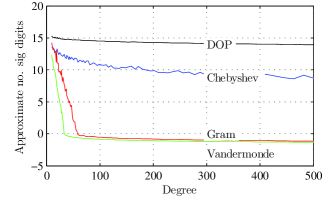
(a) Complete polynomial basis sets, i.e., $d=n-1$ where $n$ is the number of nodes.

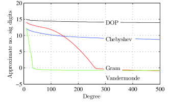
(b) Number of nodes $n=1000$, the degree of the polynomial is increasing.

Fig. 2: Estimate of the number of significant digits for different polynomials as a function of degree. DOP refers to the discrete orthonormal polynomial synthesis as proposed in this paper.

The results shown in Figure (2) indicate that the algorithm presented in this paper generates the most stable sets of polynomials. For this reason the algorithm is used for the generation of all bases required in this paper.

4.2 Initial Value Problems

In each of the following examples the analytical solution is compared with the numerical results commuted using the newly proposed method and a Runga-Kutta solution with variable step size. The ODE45 is used for comparison in all the following initial value problems.

4.2.1 IVP Example 1

The first example is a second order initial value problem with constant coefficients, the equation is [1],

$$\ddot{y}-6\,\dot{y}-9y=0,\hskip 14.22636pt\text{with},\hskip 14.22636pty(0)=10\hskip 14.22636pt\text{and}\hskip 14.22636pt\dot{y}(0)=-75.$$ (58)

in the interval $0\leq x\leq 3$ The analytical solution to this equations is,

$$y(x)=10\,e^{-3\,x}-45\,x\,{e^{-3\,x}}.$$ (59)

The analytical solution and the results of the numerical solutions are shown in Figure (3(a)). Non-uniformly spaced nodes were used, with a higher density of nodes where $\boldsymbol{y}$ has a higher first derivative. This demonstrates the possibility of generating basis functions from arbitrary nodes. The residual errors, see Figure (3(b)), with the new method is $7$ orders of magnitude smaller than with the ODE45 method.

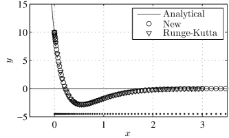
(a) Comparison of the analytical solution, the numerical solutions using the new method (with support length $l_{s}=13$, the nodes are placed $x=5z^{2}$ and $z$ has $n=85$ evenly spaced points in the interval $0\leq z\leq 1$) and using a Runge-Kutta procedure. The nodes are shown below the curve.

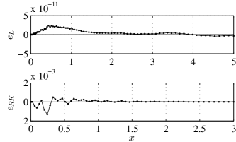
(b) Residual errors: (top) between the analytical solution and the new numerical procedure, (bottom) between the analytical solution and the numerical solution using the Runga-Kutta procedure.

Fig. 3: Computation results for the IVP Example 1 given in Equation (58).

4.2.2 IVP Example 2

The second example is a second order differential equation with variable coefficients, the equation is [1],

$$2\,x^{2}\,\ddot{y}-x\,\dot{y}-2y=0,\hskip 14.22636pt\text{with},\hskip 14.22636pty(1)=5\hskip 14.22636pt\text{and}\hskip 14.22636pt\dot{y}(1)=0.$$ (60)

in the interval $1\leq x\leq 10$. The analytical solution to this equations is,

$$y(x)=x^{2}+\frac{4}{\sqrt{x}}.$$ (61)

The comparison of the analytical solution with the numerical solutions using the new method and a Runge-Kutta procedure is shown in Figure (4). The residual error with the new method is $3$ orders of magnitude smaller that with the Runga-Kutta procedure. This example has demonstrated the ability of the proposed method to solve initial value problems with variable coefficients.

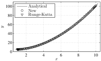
(a) Comparison of the analytical result, the numerical solutions using the new method (with support length $l_{s}=13$, there are $n=73$ evenly spaced nodes in the interval $1\leq x\leq 10$) and using a Runge-Kutta procedure.

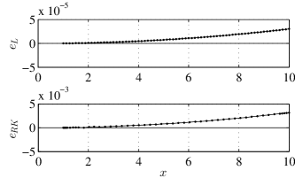
(b) Residual errors: (top) between the analytical solution and the new numerical procedure, (bottom) between the analytical solution and the numerical solution using the Runga-Kutta procedure.

Fig. 4: Computation results for the IVP example 2 given in Equation (60).

4.2.3 IVP Example 3

The third example [1] is a third order non-homogeneous differential equation with constant coefficients, the equation is,

$$\dddot{y}+3\,\ddot{y}+3\dot{y}+y=30\,\mathrm{e}^{-x}\hskip 14.22636pt\text{with},\hskip 14.22636pty(0)=3,\hskip 14.22636pt\dot{y}(0)=-3,\hskip 14.22636pt\text{and}\hskip 14.22636pt\ddot{y}(0)=-47$$ (62)

in the interval $0\leq x\leq 8$. The analytical solution to this equation is,

$$y(x)=(3-25\,x^{2}+5\,x^{3})\,\mathrm{e}^{-x}.$$ (63)

The comparison of the analytical solution with the numerical solutions using the new method and a Runge-Kutta procedure is shown in Figure (5). Once again the residual error with the new method is orders of magnitude smaller that with the Runga-Kutta procedure.

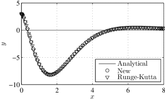
(a) Comparison of the analytical solution with, the numerical solutions using the new method (with support length $l_{s}=13$, there are $n=73$ evenly spaced nodes in the interval $0\leq x\leq 8$) and a Runge-Kutta procedure.

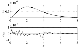
(b) Residual errors: (top) between the analytical solution and the new numerical procedure, (bottom) between the analytical solution and the numerical solution using the Runga-Kutta procedure.

Fig. 5: Computation results for the IVP Example 2 given in Equation (62).

4.3 Sturm-Liouville Problems

The test package for Sturm-Liouville Solvers [24] has been used as a source of test cases in this section.

4.3.1 Sturm-Liouville Example 1

The simplest Sturm-Liouville problem is chosen as the first example, since the analytical solution is known. This enables the investigation of the stability of the numerical computation, i.e., how many eigenvalues can be computed to a given accuracy. It is the equation of a vibrating string,

$$\ddot{y}+\lambda y=0,\hskip 14.22636pt\text{given}\hskip 14.22636pty(0)=0,\hskip 5.69054pt\text{and}\hskip 5.69054pty(\pi)=0$$ (64)

in the interval $0\leq x\leq\pi$. The analytical solution yields the analytical eigenvalues $\lambda_{k}$ and eigenfunctions $y_{k}$,

$$\lambda_{k}=k,\hskip 14.22636pty_{k}=\sin kx\hskip 14.22636pt\text{for}\hskip 14.22636ptk=1\ldots\infty.$$ (65)

The discrete solution has been computed on the interval $0\leq x\leq\pi$ sampled at the corresponding Chebyshev points; however, scaled so that the first and last points lie exactly at $0$ and $\pi$ respectively. For a given set of $n$ points $m=n/2$ constrained basis functions are computed which fulfil the boundary values. These are the admissible functions used in what is essentially a discrete equivalent of the Rayleigh-Ritz method. Two different computations $n_{1}=100$ and $n_{2}=1000$, have been performed to investigate the behavior of the solution with respect to the number of points used. A support length $l_{s}=13$ was used during the generation of the differentiating matrix. The results can be seen in Figure (6(a)) and (6(b)) respectively. The method returns the coefficients of the series of admissible functions required to generate each eigenfunction. The matrix of these coefficients is denoted by $\mathsf{R}$. We use the matrix $\mathsf{S}=\log_{10}\left\{\mathrm{abs}(\mathsf{R})\right\}$ as a visual representation for the spectrum in the figures, since at $\mathsf{S}(i,j)\approx-16$ the numerical resolution of computation environment is reached. This makes a visual recognition of when the spectrum fails simple.

With $n_{1}=100$ approximately $k_{1}=28$ and for $n_{2}=1000$ approximately $k_{2}=280$ eigenvalues could be computed with a relative error smaller than $0.1\%$. This result is significantly better than all previously reported results with matrix methods for Sturm-liouville problems [15]. This confirms the numerical stability of the approach. It also verifies that the number of eigenfunctions which can be computed to a given accuracy scales linearly with the number of nodes used.

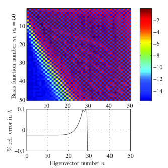
(a) Solution for $n=100$.

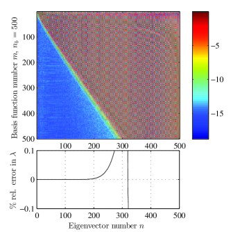
(b) Solution for $n=1000$.

Fig. 6: Solution of the Sturm-Liouville problem corresponding to the vibrating string for points. Top: spectrum of the eigenfunctions with respect to the admissible functions $(log_{10}(S)$. Bottom: The relative error in the eigenvalue $\lambda_{k}$ in $\%$.

4.3.2 Sturm-Liouville Example 2

The second example is a Mathieu differential equation; we have taken this example from [24, Problem 2, with $r=25$]. This equation arises in the vibration of elliptical membranes. We have chosen this problem because it is known to produce a pair of closely located eigenvalues; this should enable the test of the resolution of the eigenvalues computed using the proposed method. Secondly, the solution to the equation has no known analytical form, this makes numerical solutions particularly valuable. The Mathieu differential equation is,

$$\ddot{y}+2\,r\,\cos{(2x)}\,y=\lambda\,y,\hskip 14.22636pt\text{with}\hskip 14.22636pty(0)=0,\hskip 5.69054pt\text{and}\hskip 5.69054pty(\pi)=0$$ (66)

in the interval $0\leq x\leq\pi$. A Chebyshev distribution of $n=1000$ nodes are used covering the complete interval, a support length $l_{s}=13$ and $m=500$ basis functions were used for the computation. The result of the numerical computation can be seen in Figures (7(a)) and (7(b)). The pair of expected eigenvalues are computed as, $\lambda_{1}=-2.131489E+01$ and $\lambda_{2}=-2.131486E+01$.

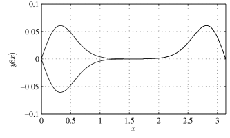
(a) The first two eigenfunctions of the Mathieu differential equation, for $r=-25$; note the negative sign for the value of $r$.

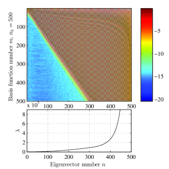
(b) Top: Rayleigh-Ritz Spectrum of the Mathieu differential equation. Bottom: the eigenvalues.

Fig. 7: Solution of the Mathieu differential equation. It is important to note that the coefficient $r$ is negative.

The results of these computations are slightly more difficult to interpret absolutely since the analytical results are not given. It can be said that the expected pair of eigenvalues have been found. Secondly, from the nature of the Rayleigh-Ritz spectrum and the corresponding computed eigenvalues, see Figure (7(b)), suggest that approximately the first $k=350$ eigenvalue are correctly computed.

4.3.3 Sturm-Liouville Example 3

This is the truncated hydrogen equation, taken from [24, Problem 4]. This is an example of s singular Sturm-Liouville equation with a limit point non-oscillatory (LPN) end point. Although only one constraint is available the equation is well conditioned, since $g(x)\rightarrow\infty$ as $x\rightarrow 0$. Highly accurate results for some eigenvalue are available for this equation [24]. These values are used to evaluate the accuracy of the computation method presented here. The differential equation is,

$$-\ddot{y}+\left(\frac{2}{x^{2}}-\frac{1}{x}\right)y=\lambda\,y,\hskip 14.22636pt\text{with}\hskip 14.22636pty(0)=LPN,\hskip 5.69054pt\text{and}\hskip 5.69054pty(1000)=0$$ (67)

in the interval $0\leq x\leq 1000$.

The computation was performed using $n=1000$ Chebyshev points on the range $0<x<1000$; further, $m=500$ basis functions were used, whereby only one constraint is applied, i.e., at $x=1000$ and a support length of $l_{s}=13$. The result of the computation are presented in Table (1). The known eigenvalues, i.e., $\lambda_{0}$, $\lambda_{9}$, $\lambda_{17}$ and $\lambda_{18}$ are comparable up the the $10^{\text{th}}$, $8^{\text{th}}$, $6^{\text{th}}$ and $5^{\text{th}}$ significant digits respectively. This indicates a high degree of accuracy, particularly considering that this is a general framework for differential equations and not a dedicated Sturm-Liouvalle solver. In [2] difficulties with oscillations at the right end point were observed for eigenvalues $\lambda_{k}$ when $k>8$, these difficulties are not observed with the methods proposed here.

	new method	known value [24]	Rel. Error
$\lambda_{0}=$	$-6.2499999978E-02$	$-6.2500000000E-02$	$3.4874503285E-10$
$\lambda_{9}=$	$-2.0661156136E-03$	$-2.0661157025E-03$	$4.3009091823E-08$
$\lambda_{17}=$	$-2.5757218232E-04$	$-2.5757359232E-04$	$5.4741446402E-06$
$\lambda_{18}=$	$2.8740937561E-05$	$2.8739013100E-05$	$-6.6963370220E-05$

Table 1: Table of eigenvalues for the truncated hydrogen equation. Comparing the numerical results obtained using the new method with the known results [24]

4.4 Boundary Value Problem Example 1

The last test is a classical Engineering boundary value problem. A cantilever with additional simple support forcing the constraint $y(0.8)=0$ is shown in Figure (8); this is an example of an inner constraint. Furthermore, the system is over constrained, since there are $5$ constraints placed on a $4^{\text{th}}$ order differential equation. It demonstrates the ability of the proposed framework to solve problems with arbitrarily placed constraints and to solve over-constrained systems. The first two admissible and eigenfunctions are shown in Figures (9(a)) and (9(b)) respectively.

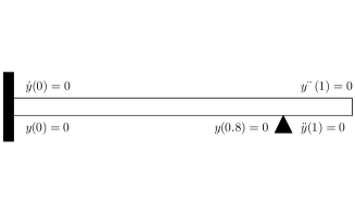
Fig. 8: Cantilever with an additional support representing an inner-value problem.

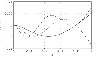
(a) The first three admissible functions for the cantilever with and additional simple support.

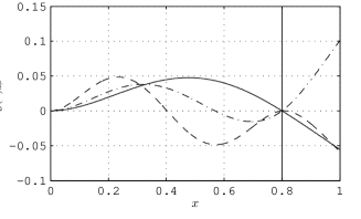
(b) The first three eigenfunctions.

Fig. 9: Admissible functions and eigenfunctions for the cantilever with additional simple support shown in Figure (8).

This computation was performed with $n=1001$ points evenly distributed along the interval $0\leq x\leq 1$, a total of $r=500$ basis functions were used and a support length $l_{s}=13$ was used for the computation of the local derivatives. The method presented for this problem is a discrete equivalent of a Rayleigh-Ritz method. The Rayleigh-Ritz coefficients for the first four eigenfunctions with respect to the first $10$ constrained basis functions are shown in Table (2).

	$\Phi(x)_{1}$	$\Phi(x)_{2}$	$\Phi(x)_{3}$	$\Phi(x)_{4}$
$c_{0}$	-0.99640	-0.06818	-0.04144	-0.00376
$c_{1}$	0.08434	-0.93235	-0.33425	-0.07821
$c_{2}$	0.00763	0.34853	-0.85504	-0.36674
$c_{3}$	-0.00317	-0.06619	0.39012	-0.82201
$c_{4}$	-0.00041	-0.01070	0.04490	-0.41659
$c_{5}$	0.00010	0.00334	-0.02068	0.04126
$c_{6}$	-0.00024	-0.00767	0.02352	-0.08609
$c_{7}$	0.00016	0.00522	-0.01475	0.02897
$c_{8}$	-0.00005	-0.00172	0.00487	-0.00615
$c_{9}$	0.00002	0.00053	-0.00157	0.00340

Table 2: The discrete Raleigh-Ritz coefficients for the first four eigenfunctions with respect to the first $10$ constrained basis functions $\mathsf{B}_{c}$ for the cantilever with additional simple support (see Figure (8)).

5 Conclusions

The successful solution od a series of initial-, boundary- and inner-value problems, with excellent results, demonstrates the general applicability of the proposed matrix framework to the solution of ODEs. The generic formulation pof the solution method as a least squares problem is very powerful, since it enables the application of the methods to many classes of problems including inverse problems.

In the case of initial value problems the least squares solution ensures that the solution has no implicit direction of solution, i.e., errors do not accumulate as the computation proceeds. Also the application of the framework to a selection of Sturm-Liouville problems has delivered results comparable with those delivered by dedicated Sturm-Liouville solvers.

The key issues in this paper which led to this success are:

1. A Lanczos process with complete reorthogonalization is used to synthesize the polynomial basis functions. This ensures highly accurate polynomial basis for the computation.

2. A correct definition of the local differentiating matrix with consistent degree of approximation over the complete support. This ensures the possibility of correctly estimating differentials at the boundary: essential for boundary and initial value problems.

3. The formulation of a method of generating orthonormal homogeneous admissible functions from constraints. The matrix containing these basis functions is ortho-normal, yielding optimal behavior in terms of error propagation. This enables the implementation of a discrete equivalent of the Rayleigh-Ritz method.

4. The formulation of the solution of the ODE as a least squares approximation; this ensure that there is no accumulation of errors.

References

- [1] R.A. Adams, Calculus: Several Variables, Pearson Addison Wesley, sixth ed., 2006.
- [2] Pierluigi Amodio and Giuseppina Settanni, A matrix method for the solution of sturm-liouville problems, Journal of Numerical Analysis, Industrial and Applied Mathematics (JNAIAM), 6 (2011), pp. 1–13.
- [3] J. Baik, Discrete orthogonal polynomials: asymptotics and applications, no. Bd. 13 in Annals of mathematics studies, Princeton University Press, 2007.
- [4] R.W Barnard, G Dahlquist, K Pearce, L Reichel, and K.C Richards, Gram polynomials and the kummer function, Journal of Approximation Theory, 94 (1998), pp. 128–143.
- [5] R. Courant, K. Friedrichs, and H. Lewy, Über die partiellen differenzengleichungen der mathematischen physik, Mathematische Annalen, 100 (1928), pp. 32–74.
- [6] R. Courant, K. Friedrichs, and H. Lewy, On the partial difference equations of mathematical physics, IBM J. Res. Dev., 11 (1967), pp. 215–234.
- [7] G.H. Golub and G. Meurant, Matrices, Moments and Quadrature with Applications, Princeton Series in Applied Mathematics, Princeton University Press, 2009.
- [8] G.H. Golub and C.F. Van Loan, Matrix Computations, The Johns Hopkins University Press, Baltimore, third ed., 1996.
- [9] J.P. Gram, Ueber die Entwickelung realer Funktionen in Reihen mittelst der Methode der kleinsten Quadrate, Journal fuer die reine und angewandte Mathematik, (1883), p. 150..157.
- [10] Khalid Hosny, Exact Legendre moment computation for gray level images, Pattern Recognition, doi:10.1016/j.patcog.2007.04.014 (2007).
- [11] Cenk Kesan, Taylor polynomial solutions of linear differential equations, Appl. Math. Comput., 142 (2003), pp. 155–165.
- [12] Yyldyray KESKYN, Onur KARAOGLU, Sema SERVY, and OTURANÇ Galip, The approximate solution of high-order linear fractional differential equations with variable coefficients in terms of generalized taylor polynomials, Mathematical and Computational Applications, Vol. 16, No. 3 (2011), pp. 617–629.
- [13] David A. Kopriva, Implementing Spectral Methods for Partial Differential Equations: Algorithms for Scientists and Engineers, Springer Publishing Company, Incorporated, 1st ed., 2009.
- [14] Nurcan Kurt and Mehmet Çevik, Polynomial solution of the single degree of freedom system by taylor matrix method, Mechanics Research Communications, 35 (2008), pp. 530 – 536.
- [15] V Ledoux, Study of special algorithms for solving Sturm-Liouville and Schrodinger equations, PhD thesis, Ghent University, 2007.
- [16] R. Mukundan, S. Ong, and P. Lee, Image analysis by Tchebichef moments, IEEE Transactions on Image Processing, 10 (2001), pp. 1357–1363.
- [17] P. O’Leary and M. Harker, An algebraic framework for discrete basis functions in computer vision, in 2008 ICVGIP, Bhubaneswar, India, 2008, IEEE, pp. 150–157.
- [18] , Discrete polynomial moments and Savitzky-Golay smoothing, in Waset Special Journal, vol. 72, 2010, pp. 439–443.
- [19] , A framework for the evaluation of inclinometer data in the measurement of structures, IEEE T. Instrumentation and Measurement, 61 (2012), pp. 1237–1251.
- [20] Igor Podlubny, Matrix approach to discrete fractional calculus, Fractional Calculus and Applied Analysis, 3 (2000), pp. 359–386.
- [21] Igor Podlubny, Aleksei Chechkin, Tomas Skovranek, YangQuan Chen, and Blas M. Vinagre Jara, Matrix approach to discrete fractional calculus ii: Partial fractional differential equations, J. Comput. Phys., 228 (2009), pp. 3137–3153.
- [22] Igor Podlubny and Blas M. Vinagre Jara, Matrix approach to discretization of ordinary and partial differential equations of arbitrary real order: The matlab toolbox, in ASME 2009 Computers and Information in Engineering Conference, San Diego, California, USA, 2009, ASME.
- [23] W.H. Press, S.A. Teukolsky, W.T. Vetterling, and B.P. Flannery, Numerical Recipes: The Art of Scientific Computing, Cambridge University Press, Cambridge, third ed., 2007.
- [24] J. D. Pryce, A test package for Sturm-Liouville solvers, ACM Trans. Math. Softw., 25 (1999), pp. 21–57.
- [25] A. Savitzky and M. Golay, Smoothing and differentiation of data by simplified least squares procedures, Analytical Chemistry, 36 (8) (1964), p. 1627..1639.
- [26] Mehmet Sezer and Mehmet Kaynak, Chebyshev polynomial solutions of linear differential equations, International Journal of Mathematical Education in Science and Technology, 27 (1996), pp. 607–618.
- [27] J. Wilkinson, Modern error analysis, SIAM Review, 13 (1971), pp. 548–568.
- [28] G.Y. Yang, H.Z. Shu, G.N. C. Han, and L.M. Luo, Efficient Legendre moment computation for grey level images, Pattern Recognition, 39 (2006), pp. 74–80.
- [29] Pew-Thian Yap and Paramesran Raveendren, Image analysis by Krawtchouk moments, IEEE Transactions on Image Processing, 12 (2003), pp. 1367–1377.
- [30] , An efficient method for the computation of Legendre moments, IEEE Transactions on Pattern Analysis and Maschine Intelligence, 27 (2005), pp. 1996–2002.
- [31] Hongquing Zhu, Huazhong Shu, Jun Liang, Limin Luo, and Jean-Louis Coatrieus, Image analysis by discrete orthogonal Racah moments, Signal Processing, 87 (2007), pp. 687–708.
- [32] Hongquing Zhu, Huazhong Shu, Jian Zhou, Limin Luo, and Jean-Louis Coatrieus, Image analysis by discrete orthogonal Racah moments, Pattern Recongition Letters, doi:10.1016/j.patrec.2007.04.013 (2007).